The Role of Stochastic Models in Interpreting the Origins of Biological Chirality

Department of Inorganic and Analytical Chemistry, University of Debrecen, P.O.B. 21, Debrecen, H-4010 Hungary
Symmetry 2010, 2(2), 767-798; https://doi.org/10.3390/sym2020767
Submission received: 1 March 2010
/
Revised: 29 March 2010
/
Accepted: 6 April 2010
/
Published: 12 April 2010
(This article belongs to the Special Issue Symmetry of Life and Homochirality)
Abstract
:This review summarizes recent stochastic modeling efforts in the theoretical research aimed at interpreting the origins of biological chirality. Stochastic kinetic models, especially those based on the continuous time discrete state approach, have great potential in modeling absolute asymmetric reactions, experimental examples of which have been reported in the past decade. An overview of the relevant mathematical background is given and several examples are presented to show how the significant numerical problems characteristic of the use of stochastic models can be overcome by non-trivial, but elementary algebra. In these stochastic models, a particulate view of matter is used rather than the concentration-based view of traditional chemical kinetics using continuous functions to describe the properties system. This has the advantage of giving adequate description of single-molecule events, which were probably important in the origin of biological chirality. The presented models can interpret and predict the random distribution of enantiomeric excess among repetitive experiments, which is the most striking feature of absolute asymmetric reactions. It is argued that the use of the stochastic kinetic approach should be much more widespread in the relevant literature.
1. Introduction
Ever since the discovery of molecular chirality, the apparently inherent asymmetric nature of biologically important compounds has attracted the attention of thousands of scientists. In a special issue celebrating the 125th birthday of Science magazine in 2005, its editors mentioned this problem in a list of 125 most important scientific puzzles that are driving basic experimental and theoretical research [1]. The last comprehensive book on this subject was published in 2004 [2]. It is well known that L-amino acids and D-carbohydrates dominate in life on Earth as we know it. There are very strong reasons to believe that there was no molecular asymmetry in the Universe at some primordial point in time. Therefore, the significant asymmetry of chemical compounds observed today must have been generated at some point by a natural process (probably on Earth), which is thought to be part of evolutionary history. As the very fundamental building blocks of life themselves are chiral, it is just pure common sense to assume that some asymmetry was first generated by pre-biotic chemical processes and later maintained and quite possibly further amplified by biological phenomena. This initial pre-biotic generation of asymmetry has been the subject of extensive theoretical speculation for a long time. Some relevant experimental information reported in the last two decades, especially the discovery of the Soai reaction, has intensified and given new directions to modeling efforts. Asymmetric autocatalysis lies in the center of these efforts, which provides a very attractive interpretation of the eventual origin of biological chirality as, unlike all other proposed explanations, it can be modeled without the inclusion of unknown external factors.
Absolute asymmetric synthesis, in which optically active material is prepared from nonchiral starting materials in the absence of any optically active catalysts or reagents may follow from enantioselective autocatalysis. It should be noted that the requirement for excluding optically active catalysts will be used here in a broad sense that is not limited to chemicals, but also includes circularly polarized light or other radiation, chiral surfaces, or generally any other possible asymmetric external influence that may affect the outcome of a chemical reaction [3]. The traditional way of interpreting absolute asymmetric synthesis relies on the mathematical background of deterministic kinetics and small initial fluctuations, which can never be described based on the deterministic models. The usual course of such interpretations is to show that a particular scheme leads to the formation of huge enantiomeric excesses starting form a minute initial imbalance of enantiomers. Although this is a sound qualitative interpretation, its quantification would require the full description of initial fluctuations, which is not possible within the realms of the deterministic kinetic approach. Consequently, by its very foundations, such a method will be unsuitable for predicting enantiomeric excess distributions observed in experimental examples of absolute asymmetric synthesis. This review will summarize recent stochastic attempts which have been developed to meet the formidable challenges posed by the advance of experimental work in the field.
It should also be noted that the question of how one or other enantiomer built up a reasonable excess from a symmetric initial state during pre-biotic evolutionary processes and reached its present-day levels is quite distinct from the question why exactly the enantiomers in excess today (L-amino acids and D-carbohydrates) were selected by evolution. All reliable information known today points to the direction that this choice between enantiomers was a random one in nature. In other words, life based on D-amino acids and L-carbohydrates would function just as well as the one we are familiar with. Therefore, efforts to answer the first question will be summarized in this article. Only the results of modeling studies will be stated here, the mathematical proofs can be found in the original studies. Mathematical notations will be in agreement with the system used on the web site Wolfram Mathworld [4]. Therefore, equations appearing in the original articles had to be re-formulated from time to time for internal consistency within this review.
2. Stochastic Experimental Observations Relevant for Chirality and Autocatalysis
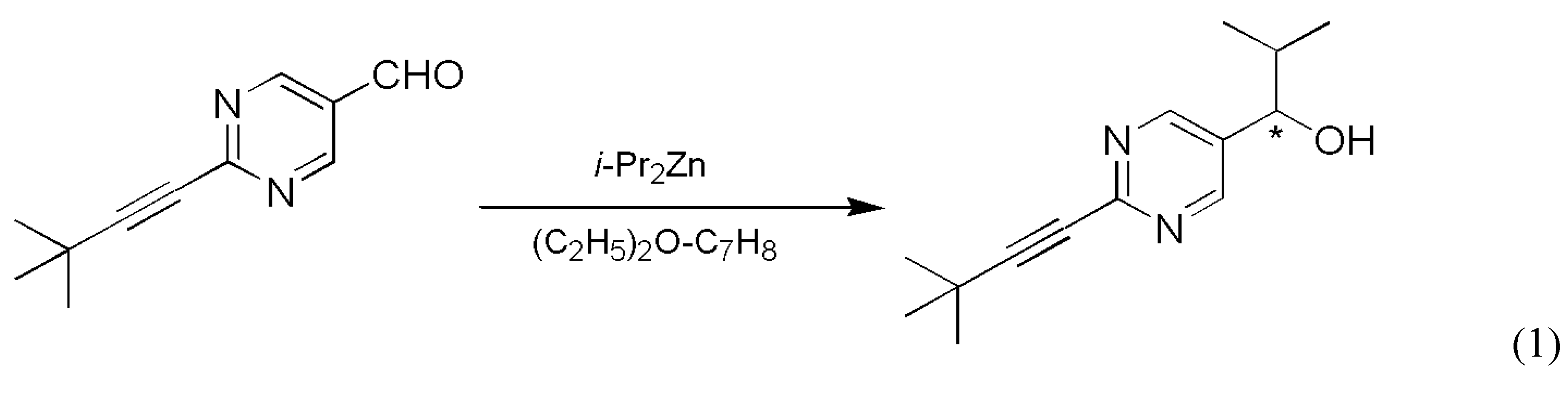
The reaction most often cited and analyzed in relation to enantioselective autocatalysis is the Soai reaction, which involves a carbon-carbon bond formation reaction using an organozinc compound (Scheme 1).
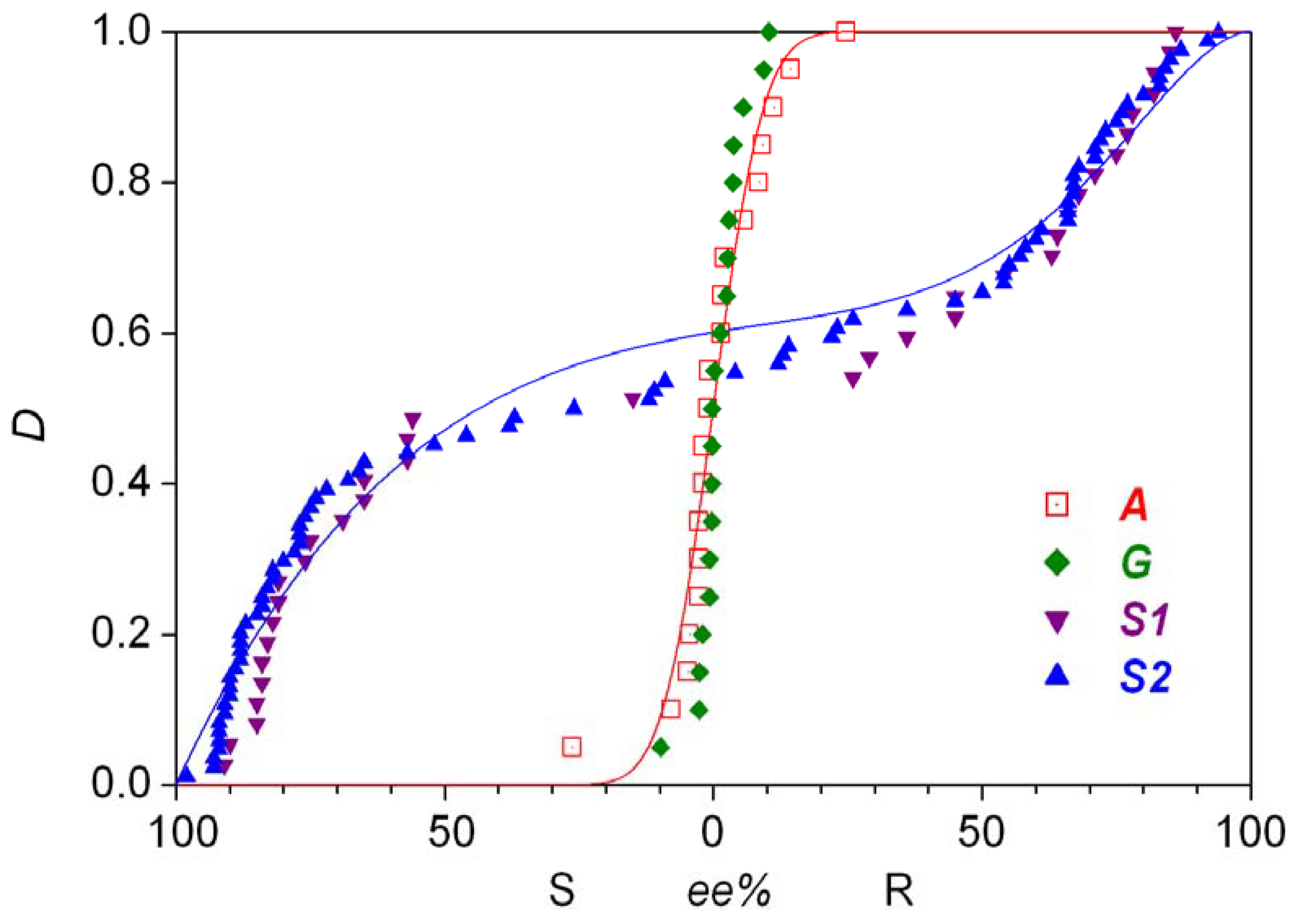
The Soai group published the first solid results about enantioselective autocatalysis in this process in 1995 [5]. A follow-up patent document reported the first experimental example of absolute asymmetric synthesis [6] with a slightly different substrate: a simple a methyl group was the unreactive side chain trans to the carbaldehyde group on the pyrimidyne ring. Later, a two-step synthetic process was published in which enormous random fluctuations in the enantiopurity of the product were observed and the stochastic nature of the process was demonstrated by 37 repetitive experiments [7]. The distribution is shown in Figure 1 as series S1. The same reaction was also carried out under somewhat different conditions, most notably the presence of nonchiral silica gel was a new element [8]. With 84 repetitive experiments, this work has yielded the most extensive experimentally determined stochastic data set known to date, which is shown in Figure 1 as series S2. Later publications also demonstrated that 12C/13C and hydrogen isotope chirality can also be amplified by the Soai reaction [9,10]. A review of the experimental results was published within the last year [11].
Gridnev et al. [12] basically reproduced these findings reported from the Soai group. Their reaction was only different from the one shown in Equation 2 by the replacement of the quaternary carbon atom by a silicon atom at the non-reactive side chain on the aromatic ring [12]. In that work, 20 repetitive experiments gave the distribution shown as series G in Figure 1. The enantiomeric excesses obtained are smaller than in S1 and S2, but this could be attributable to the somewhat different substrates and the different reaction conditions.
Singleton and Vo [13] reported the results of 48 synthetic experiments in the same reaction the patent from the Soai group studied [6]. These included a lot of thoughtfully devised variation of experimental conditions from one experiment to another, which were very useful to make qualitative points about the nature of the process but also rendered any statistical attempts to evaluate the data set futile. The authors brought up the possibility of a significant role played by minor chiral impurities in the system, an important question that, as will be explained in later parts of this review, can actually be addressed through statistical analysis. A later paper from the same pair of authors compared 81 separate experiments in the same system [14], some of them using the enantioenriched product as a chiral additive. The enantiomeric excess values were not specified in this report as the amplification was typically repeated until a pre-set excess of one of the two optical isomers were reached.
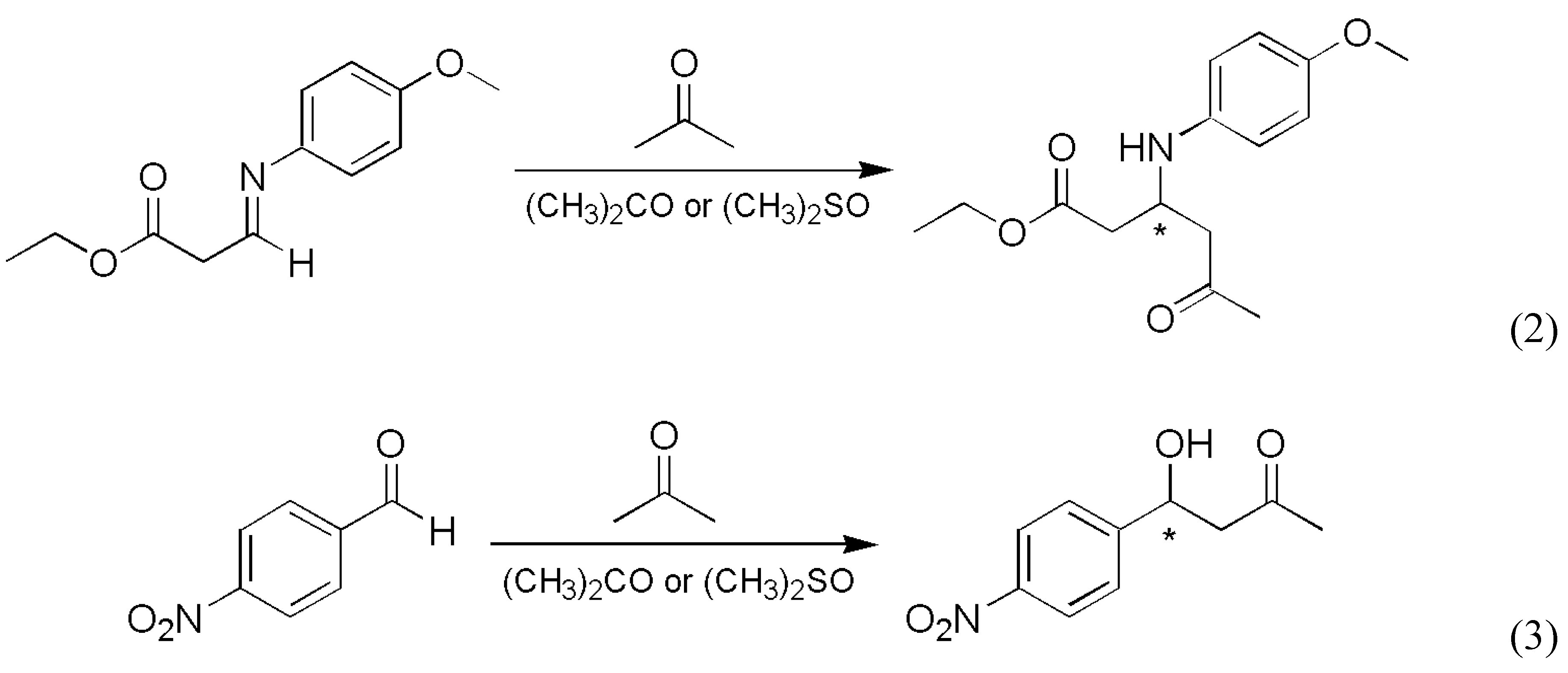
Mauksch et al. reported random generation of enantiomeric excesses in Mannich and aldol reactions [15] (Scheme 2).
This study only demonstrated the existence of a stochastic element in the studied process but did not provide enough repetitive experiments to carry out any meaningful statistical analysis. Even based on the limited data set published [15], there is strong indication that the preference for the R and S enantiomers formed is not 50-50 % in this case, which may be attributed to practical imperfections in the experiments rather than an inherent stochastic nature of the system.
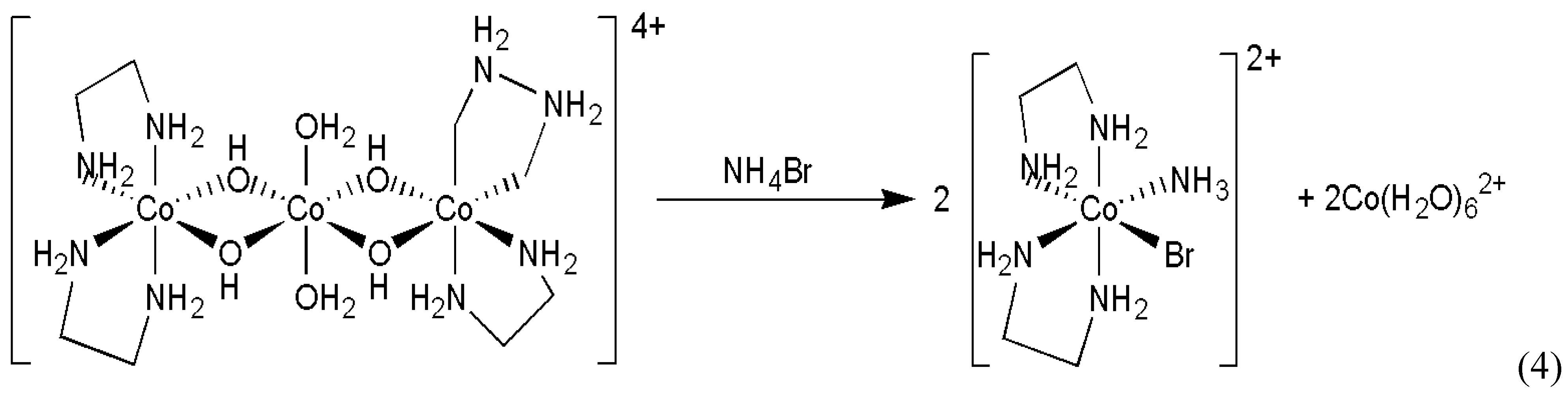
In a completely different inorganic reaction, quite substantial random fluctuations were reported in the cleavage of a Co(III)(μ-OH)2Co(II)(μ-OH)2Co(III) type trinuclear cobalt complex [16] (Scheme 3).
The product octahedral cobalt(III) complex is chiral due to the presence of the ethylenediamine ligands and its enantiomers can be resolved because of its inertness. Small, but clearly detectable random fluctuation was observed in the enantiomeric excess of the chiral product in a series of experiments which involved 20 repetitions of identical procedures. The experimental distribution of determined enantiomeric excess obtained is displayed in Figure 1 as series A. Some earlier and later efforts were also published connected to this particular reaction [17,18,19].
A major shortcoming of the experimental data reported about absolute asymmetric synthesis is that they were rather focused on the synthetic aspects and the final formation of large random enantiomeric excesses without giving much attention to meaningful kinetic monitoring of the reactions. This is important because the stochastic aspects must be observed in the kinetics of these processes as well. However, experimental examples of detectable stochastic kinetic effects in autocatalytic reactions not involving any chiral material were provided by the pioneering work of Nagypál and Epstein [20,21]. The first such process studied was the reaction between chlorite ion and thiosulfate ion, the stoichiometry of which can be described by the combination of the following two reactions depending on the experimental conditions [20]:
4S2O32− + ClO2− + 2H2O = 2S4O62− + 4OH− + Cl−
S2O32− + 2ClO2− + H2O = 2SO42− + 2Cl− + 2H+
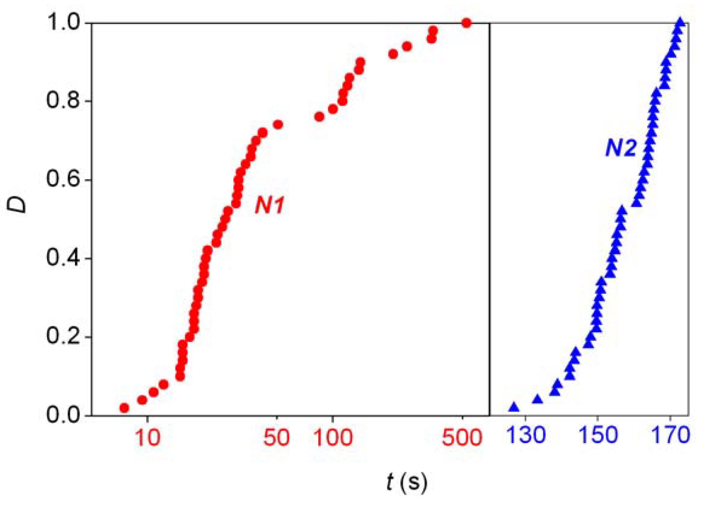
In unbuffered solution with a pH around 11, the reaction shows Landolt or “clock reaction” characteristics in a rigorous sense [22], whereby an initial increase in pH is followed by an abrupt drop. The Landolt time was shown to display stochastic fluctuations and a statistically meaningful study (at least 50 repetitions of identical experiments for characterizing each distribution) at various experimental conditions, including initial concentrations, stirring rates, reactant volumes and medium temperatures was carried out in a systematic manner. The distribution of Landolt times from one of the experimental series is shown by curve N1 in Figure 2. A similar full-scale stochastic distribution study was also reported in the reaction between chlorite ion and iodide ion [21], where the gradual buildup in iodine is followed by its sudden disappearance in an acetate-buffered solution at pH ~ 4 because of the coupling of the following two processes:
4I− + ClO2− + 4H+ = 2I2 + Cl− + 2H2O
I2 + 5ClO2− + 2H2O = 4IO3− + 5Cl− + 4H+
There are numerous examples of chiral symmetry breaking during crystallization, which are somewhat similar to the homogeneous examples listed above. It should be made clear that a similar phenomenon, spontaneous resolution in crystallization is quite different conceptually. In this latter process, which is the historical way of the discovery of chirality [23,24], an existing racemic mixture (such as tartaric acid) is crystallized into enantiopure crystals and there is no need for any random elements. In chiral symmetry breaking crystallization, the source of chirality is the formation of enantiomorfic crystals (similar to quartz) and the initial substance may not be chiral at all. The stochastic nature was nicely demonstrated in the crystallization of sodium chlorate [25] and amino acids glutamic acid and lysine [26]. Relevant results have been reviewed from several different aspects [27,28,29,30,31,32] and extended to phase transitions in general [33,34].
3. Statistical Tests without Chemical Models
A limited analysis of the experimentally measured statistical distributions is possible without having any particular chemical mechanism in mind. As there is no limit on the number of repetitive experiments one can do, comparisons are routinely done with continuous statistical distributions. Data set A displayed in Figure 1 has been shown to adhere to normal distribution [35]. The probability and distribution functions are as follows:
The distributions are given here in terms of the molar fraction of the R isomer (xR), which is connected to the percentage enantiomeric excess (ee%) with the following simple formula:
If xR < 0.5, the S enantiomer is in excess, conversely, the R enantiomer is in excess for xR > 0.5. Distribution A shown in Figure 1, which is in a narrow range around the enantiomeric excess of zero, was assumed to be centered around the racemic mixture. etc. the expectation μ = 0.5 was pre-set and a standard deviation of σ = 0.037 was found to fit the experimental data best. [35] (Note that the value of σ was reported erroneously by a multiplication factor of in the original article [35].) The theoretical distribution is shown as a solid line in Figure 1. The normal distribution approximates the experimental measurements in their range well, but the adherence should not be taken literally outside the range of experimental data, as Equation 9 and Equation 10 would give nonzero probabilities (2.1 × 10−42 in this case) for the impossible case where the enantiomeric excess is larger than 100%. Later distributions appearing in this review are free from this problem because they are only interpreted on a limited interval of real numbers. The good fit to the normal distribution in the case of data set A is not unexpected given the relatively minor fluctuations measured.
A combined beta distribution has been proposed to interpret the experimental distributions found in the Soai reaction with the following probability and distribution functions [36]:
In these formulae, Γ(a) is the gamma function, B(xR,a,b) is the incomplete beta function and B(a,b) is the complete beta function. As shown in Figure 1, a good-looking fit to data set S2 could be obtained with the values a = 2, b = 10, c = 5, d = 1 and w = 0.382. (This is slightly different order from the one reported in the original work [36] as the left part of Figure 1 refers to cases where the S isomer is in excess.) The probability function based on Equation 11 was compared [36] with a histogram constructed based on the published data [8]. This is an unfortunate practice as it includes some rather arbitrary categorization, the dangers of which have already been pointed out [35]. To demonstrate the goodness of fit, a comparison between distribution functions seems to be the best practice thus far [20,21,35,37,38]. Furthermore, it should be noted that distribution (12) is clearly asymmetric, the significance of which will be discussed later along with distributions giving a visually more attractive fit to data set S2 with fewer parameters, both symmetric and asymmetric, based on chemical models [35,37,38].
The symmetry of the experimentally measured distributions can be tested independently of any chemical considerations [35,38,39,40,41]. The Wilcoxon rank sum test showed that there is no significant asymmetry in data sets A and S1 [35]. Data set S2, however, was shown to be significantly asymmetric by both the simple Wilcoxon rank sum test [38] and by more advanced statistical evaluation [39,40,41]. Furthermore, it was shown that (a) distributions S1 and S2 are non-binomial (hence not normal), (b) S2 cannot be described by a symmetric beta distribution [39]. During the present general analysis, it should be pointed out that property (b) also follows from the fact that distribution S2 is significantly asymmetric.
4. Model-Based Stochastic Kinetic Approaches
In many fields of science, it seems evident that stochastic experimental phenomena must be interpreted by stochastic models. Unfortunately, this is not the case in the quest for the origins of biological chirality where published papers based on the deterministic approach outnumber stochastic attempts by at least two orders of magnitude. The reason for this rather puzzling insufficiency might be that the problem is distinctly chemical, but chemists, unlike physicist and biologists, are usually trained all over the world without much exposure to basic probability theory. It should be made clear that the stochastic approach to chemical kinetics is already well established. As early as 1940, Delbrück noted that inherent stochastic phenomena are expected under certain conditions in autocatalytic reactions dealing with macroscopic amounts of substance [42], an insight which was experimentally verified in work already discussed in Section 2 [20,21]. Stochastic approaches to chemical kinetics were nicely developed and summarized by Érdi and Tóth [43,44]. Stochastic kinetics is routinely used in physics to evaluate measurements studying rare radioactive decays [45] and stochastic considerations are also routine in the physical analysis of symmetry breaking and restoration [46].
First of all, a difference between irreproducibility and inherent stochastic nature should be clearly made in chemical systems [35,47]. Both phenomena imply random variations in experimental results, but the underlying reasons are very different. Irreproducibility is caused by insufficiently controlled external factors, e.g. impurities, environmental temperature or pressure fluctuations, light absorption, etc. In such cases, recognizing the important external factor and improving its control will result in greatly reduced random variations. Inherent stochastic nature, e.g. a movement of an electron on a quantum mechanical level, is due to the laws of nature and no refinement of experimental control will remove it. However, the laws governing the behavior of the system must be reflected in experimental results. In relation to enantioselective autocatalysis, four criteria were proposed to differentiate between irreproducibility and stochastic nature [35]:
- Traditional demonstration of autocatalysis by experiments using the initial addition of enantiomer-enriched products. Autocatalysis is a possible reason for inherent stochastic nature in macroscopic experiments, but autocatalysis can be tested under circumstances where no stochastic behavior is expected.
- Analysis of the stochastic distribution of enantiomers through a high number (preferably > 50) of repetitive experiments. In most cases, symmetric distributions are expected and a significantly asymmetric experimental distribution may point to an uncontrolled (most often also unidentified) but significant external influence.
- Detection of random fluctuations in reaction time. If a random enantiomeric distribution is indeed caused by inherent stochastic nature, the time-dependent kinetics should also show random variations.
- The final distribution of enantiomeric excess and reaction times should be dependent on the overall volume even if the very same initial concentrations are used. This is a theoretically well known phenomenon that is usually expressed by saying that stochastic kinetics is equivalent to deterministic kinetics at the limit of infinite volume [48].
It should be noted that the eventual inevitability of the use of stochastic kinetics for certain problems can be forcefully demonstrated by pointing out the insufficiencies of the deterministic approach. Consider the following pair of simultaneous differential equations, which give the deterministic description for simple first-order enantioselective autocatalysis transforming a nonchiral A molecule into BR and BS enantiomers of a chiral B product [37]:
In these equations, ku and kc represent rate constants, [A]0 is the initial concentration of reactant A, mass conservation is assumed to hold for the sum of substances A and B, [BR] and [BS] give the concentrations of the two enantiomers as a function of time. These equations can be solved analytically [37]. Parameters [A]0 = 0.2 M, ku = 10−15 s−1 and kc = 108 M−1s−1 will be used in the example. The rate constants have been chosen so that the deterministic approach leads to an irresolvable contradiction. However, the values assumed for ku and kc are by no means impossible from a practical point of view. The value of ku corresponds to an extremely slow first-order process, whereas the other path represents a fast second-order reaction with a kc that is about two orders of magnitude lower than the diffusion-controlled limit. If there is absolutely no chiral material present initially, etc. [BR](t = 0) = [BS](t = 0) = 0, the symmetry of Equation 14 and Equation 15 ensures that the final state will also be symmetric with [BR](t → ∞) = [BS](t → ∞) = 0.1 M. However, the very same parameters with the initial condition representing a single BR molecule in 10 cm3 of overall reaction solution, [BR](t = 0) = 1.66 × 10⁻²² M and [BS](t = 0) = 0 will predict [BR](t → ∞) = 0.1943 M and [BS](t → ∞) = 0.0057 M. This is a huge contradiction as the first molecule formed in the system must be either BR or BS, there is no middle ground there, so the system must go through either the asymmetric state mentioned in the previous analysis or its mirror-image counterpart [BR](t = 0) = 0 and [BS](t = 0) = 1.66 × 10⁻²² M. Therefore, the final enantiomeric balance predicted based on the initial state and on an intermediate state that the system must necessarily go through contradict each other. An apparent escape of this contradiction might be thinking that it is always imperative for two molecules of B (one BR and one BS) to form every time at exactly the same moment, but this would be tantamount to denying the very foundations of atomistic theory (independency of individual particles). In probabilistic terms, two molecules formed at exactly the same time is the surprising, but statistically well known case of an event that has zero probability but not impossible.
This example clearly demonstrates that the major insufficiency of the deterministic kinetic approach is its reliance on continuous concentration-time functions. As the usual number of particles dealt with in chemistry is very high (about 1020 or higher), this approach is quite satisfactory for the overwhelming majority of cases. However, one should be vigilant about cases where it cannot work exactly because of the initial (and often tacit) assumptions. As the above example shows, it would be a mistake to think that the stochastic kinetic effects arising from the particulate nature of matter can only be significant at unpracticably low molecule numbers, autocatalysis and its consequences clearly prove the opposite.
There are several different methods to account for stochastic elements in chemical kinetics. The most important is called the continuous time discrete state (CDS) approach and will be discussed in the remaining sections of this review. In this section, however, a brief summary of different attempts will be provided.
It has been pointed out several times that a racemic mixture in dynamic equilibrium does not contain strictly the same number of both enantiomer molecules [3,40,49,50,51,52,53,54,55,56,57,58,59]. A racemic mixture in general can be characterized by a binomial distribution. This could be well understood within the concepts of the CDS approach but will be discussed in this Section as it has no kinetic relevance at all. The binomial distribution for the case where some inherent asymmetry between enantiomers is also allowed takes the following form [54]:
P(r,s) is the probability of obtaining exactly r molecules of the R (more stable) enantiomer and s molecules of the S (less stable) enantiomer. Parameter ε is characteristic of the degree of inherent asymmetry (ε ≤ 0.5). Any formula given in the following equations can be used for the perfectly symmetric case with setting ε = 0. The importance of calculations in the asymmetric case was that the possible consequences of the parity violation energy difference had to be analyzed. Parameter ε can be calculated from the inherent energy difference (ΔE) between the enantiomers [54], the temperature (T) and the universal gas constant (R) as follows:
For a given overall number of chiral molecules N (= r + s), the expectations and standard deviation of the of the distribution given in Equation 16 can be given as:
Present theoretical predictions [60], which have been especially carefully checked for the product of the Soai reaction [61], show that ΔE following from the phenomenon of parity violation should be around 10−13 J mol−1 giving an estimate of 10−17 for ε at room temperature. It has been pointed out several times [54,58,59] that for 1 mol of chiral molecules (N = 6 × 10²³) these values lead to an expected excess of the more stable (R in this case) enantiomer (6 × 10⁶) that is much smaller than the standard deviation (1.9 × 10¹¹). The present author believes that any role played by the parity violation energy differences is highly unlikely based on this simple line of thought alone.
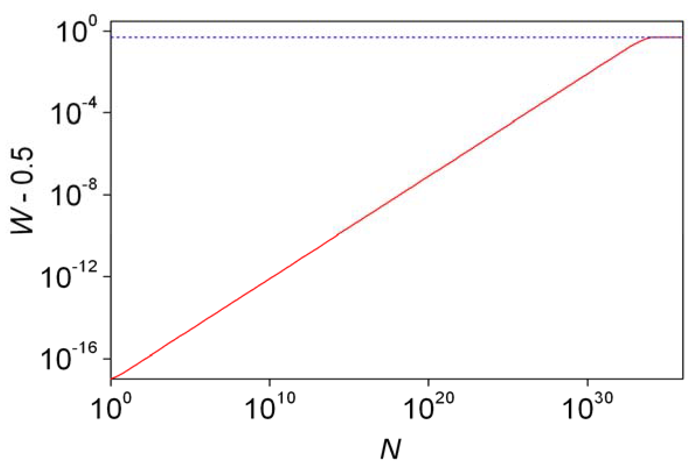
As a further stochastic analysis, the probability of forming the more stable enantiomer in excess (W) was defined and calculated analytically [54]. Odd and even numbers of N had to be treated separately, which is understandable as for an odd number of molecules it is impossible to have a perfectly racemic mixture (r = s) by default. With a unified treatment, a new parameter l is introduced which is given as follows:
The probability W can be given as [47]:
The last part of Equation 21 is an approximation that only works well for W values smaller than 0.6. Probabilities W (actually W – 0.5 to have a practical logarithmic scale) are shown as a function of N in Figure 3. Further characteristics of the distribution have been estimated. The probability of forming a perfectly racemic (r = s) mixture can be found from Equation 16 by substituting r = s [46]. Mills [43] and later authors [3,46,48] defined and used the another descriptor, ee%½. This is basically the ee% value where the distribution function takes the value of 0.5. Enantiomeric excesses higher than this threshold value (ee%½) are expected to form with 50% probability. The following simple rule was deduced based on considerations using the properties of the normal distribution [3,49,52,55]:
For better characterization, it would be good to calculate the expectation and standard deviation for ee, which does not seem to have been done in any of the earlier works. Unpublished conjectures of the present author are the following:
Turning now to stochastic non-CDS approaches to kinetics, Todorović et al. [62] investigated a slightly modified version of the classic Frank model [63]. Rather than considering the effect of individual molecules, the rate constants in the stochastic model were assumed to show stochastic fluctuations. Symmetric pairs of reactions producing different enantiomers of the same molecule were assumed to have uncorrelated fluctuations, which was the eventual origin of symmetry breaking within the deterministic rate equations. The differential equations were solved numerically with a fourth-order Runge–Kutta procedure using a pre-set finite step size with the rate constants varied according to a uniformly distributed random variables after each step. Conclusions were drawn based on regularities observed after several series of calculations started from identical, strictly non-chiral initial conditions. The results showed that the separation time, which is the shortest time after which the sign of the enantiomeric excess remains the same, was independent of the magnitude of fluctuations in the rate constant. In contrast, the parting time, defined as the moment at which the enantiomeric excess attains 1% of its limit for the first time, was a linear, decreasing function of the logarithm of the magnitude of the fluctuations in the rate constants. The drawback of this approach is that it assumes uncorrelated fluctuations in the values of rate constants which should be enantiomeric mirror-image pairs and the origin of these fluctuations, which remained unspecified in the original work [62], may only be external. Consequently, this is a description of irreproducibility rather than inherent stochastic nature.
Cruz et al. also analyzed the effect of noise on the Frank model, but the random variables were introduced directly into the deterministic rate equations [64]. In fact, this is not very fortunate as it makes the questionable assumption that the rate equations themselves, and not the variables and parameters appearing in them, are subject to noise. Uncorrelated Gaussian white noise was included in the calculation of rates and the equations were solved by a fourth-order Runge-Kutta method with pre-determined step size. With small noise amplitudes, no formation of significant enantiomeric excess was observed. When the noise amplitude was higher than a critical value, the enantiomeric excess converged to 100% in the numerical simulations. The article makes no clear statement in this regard, but implies that the added noises considered in the different rates were not scaled, etc. very different rates were subjected to noise of the same magnitude.
Rivera Islas et al. [65] studied three schemes related to the Frank model with deterministic simulations in order to study mirror-symmetry breaking. Surprisingly, they found spontaneous generation of sizable but unpredictable enantiomeric excesses starting from a completely nonchiral starting state. This effect primarily depended on the details of the numerical integrator used and was a consequence of the dynamic instability of the studied kinetic scheme. Micskei et al. made very similar observations [66] while studying an oscillatory model of the Soai reaction in a semibatch reactor. They proposed that the inherent numerical error of the integrator method might be a model of the statistical fluctuations. However, the present author feels that it is very questionable to draw chemical conclusions from effects that are admittedly caused by the insufficiency of the numerical method used to solve mathematical equations.
Hochberg and Zorzano [67] developed Langevin-type equations based on field theoretic techniques to describe inherent spatio-temporal fluctuations in the Frank model. Numerical simulations in two spatial dimensions showed that an enantiopure state can in fact form from strictly racemic initial conditions. The eventual origin of this symmetry breaking is the internal fluctuations in particle density. Although this is a valid stochastic method, it still works based on continuous concentrations rather than discrete particle numbers. In a very well stirred reactor, the authors expected the round-off errors of the numerical calculations to be a decisive factor similarly the earlier results [65]. A later study from Hochberg and Zorzano also used the previous approach to study critical properties of the Frank Model [68]. An unstable, non-chiral fixed point, a pair of stable homochiral fixed points and racemic saddle point were characterized.
In more recent developments, Hochberg adopted an analytic perturbation method, which provides potentials associated with a wide class of stochastic partial differential equations, to introduce an effective potential for the Frank model [69,70]. This was also used to study the effects of external noise. Weak noise seemed to erase homochirality and stronger noise was needed to do the same when the system contained some chiral bias. Calculations were done in well mixed systems and also taking the effect of two dimensional diffusion into account.
Gleiser and Walker used limited stochastic elements in their study of a generalized autocatalytic model for chiral polymerization [71]. The system developed in this work was at some point coupled to a source of noise through a stochastic spatiotemporal Langevin equation to achieve small initial spatial fluctuations in the concentrations. However, the role of the stochastic approach and conclusions based on it are of secondary importance in this work.
5. The Continuous Time Discrete State Approach
5.1. General Characterization
The continuous time discrete state (CDS) stochastic kinetic approach is probably the closest to the currently accepted particle-based view of matter. The mathematics of CDS is authoratively summarized in the book of Érdi and Tóth [44], and only the basic information necessary to understand the forthcoming discussion is given here. In CDS, the system is characterized by giving the numbers of each particle present. Instead of giving the concentrations as a function of time, the changes are described by giving the probabilities of all possible states as a function of time. A differential equation for the probability of every state is written based on the kinetic scheme. These Kolmogorov-like equations are referred to as the master equation of the process. The differential equations obtained in CDS, unlike in the deterministic approach, are all linear and can in principle be solved analytically. However, this analytical way of solving them is usually hindered by the fact that there are orders of magnitude more possible states than concentrations in the deterministic approach. Laplace transforms are often useful in the analytical solution of the master equation. The master equation can also be stated with matrix formalism. For this, an enumerating function, f, is needed first, which gives a single and unique whole number to every possible state without repetitions or omissions. Therefore, if the number of possible states is M, f(c1, c2, c3, ..., ck) should take the values 1, 2, ..., M with c1, c2, c3,..., ck being the molecule numbers for molecule types 1, 2, 3, ..., k. If P is defined as a vector containing the probabilities of all states in the order of the values of the enumerating function, the master equation can be formulated as follows:
Matrix is the transition probability matrix (sometimes also called evolution matrix), the elements of which fall into two categories. Elements in the main diagonal are all negative and give the probability of the disappearance of each state. Elements outside the main diagonal in the ith row and jth column give the probabilities of forming state i from state j. If all possible states are enumerated, all column sums in are 0, therefore is a singular matrix. For systems that have no elements of reversibility, etc. the same state cannot occur twice during the course of the process, it is often informative to calculate the probability (Q) of a given state ever occurring during the entire course of the reaction. It can be shown that Q is related to function P is follows:
It should be noted that the CDS approach is superior to the deterministic kinetic approach because it allows for the particulate nature of matter without making any extra assumptions not already present in the deterministic approach. Every conclusion drawn with the deterministic approach can be reached as a limiting case of the CDS approach for very high particle numbers in very high volumes [48,72].
There is a simple relationship connecting stochastic (κ) and deterministic (k) rate constants, which is useful in comparing the two approaches. The formula only contains the Avogadro constant (NA), the overall volume (V) of the system and the order of the rate constant (i):
This relationship is actually the very origin of test 4 introduced in Section 4 to identify inherent stochastic nature in absolute asymmetric synthesis.
Despite its wide possible application range, the CDS kinetic approach is quite rare in the chemical literature. In addition to the issues connected to the way chemists are trained, a more objective reason for this lack of general interest is that CDS is much more computationally intensive than the deterministic kinetic approach. Although Equation 25 is a simple first-order differential equation, which can be solved analytically for any circumstances, transforming the solution into a form that is useful for comparing with experimental results is a quite separate and much more difficult issue. In addition, the concept of reproducibility is central in chemistry, so any hint of substantial random variations in experimental results is a solid reason for abandoning a project in most chemistry laboratories. One might actually wonder how much good stochastic experimental data could have remained unpublished through the last decades.
One minor exception from underreporting stochastic experimental observations is the field of enzyme catalysis. A stochastic solution to the Michaelis-Menten scheme has been described from different aspects [73,74,75] and experimental observations related to single-enzyme catalysis have also been published [76,77].
5.2. Simple Autocatalytic Schemes
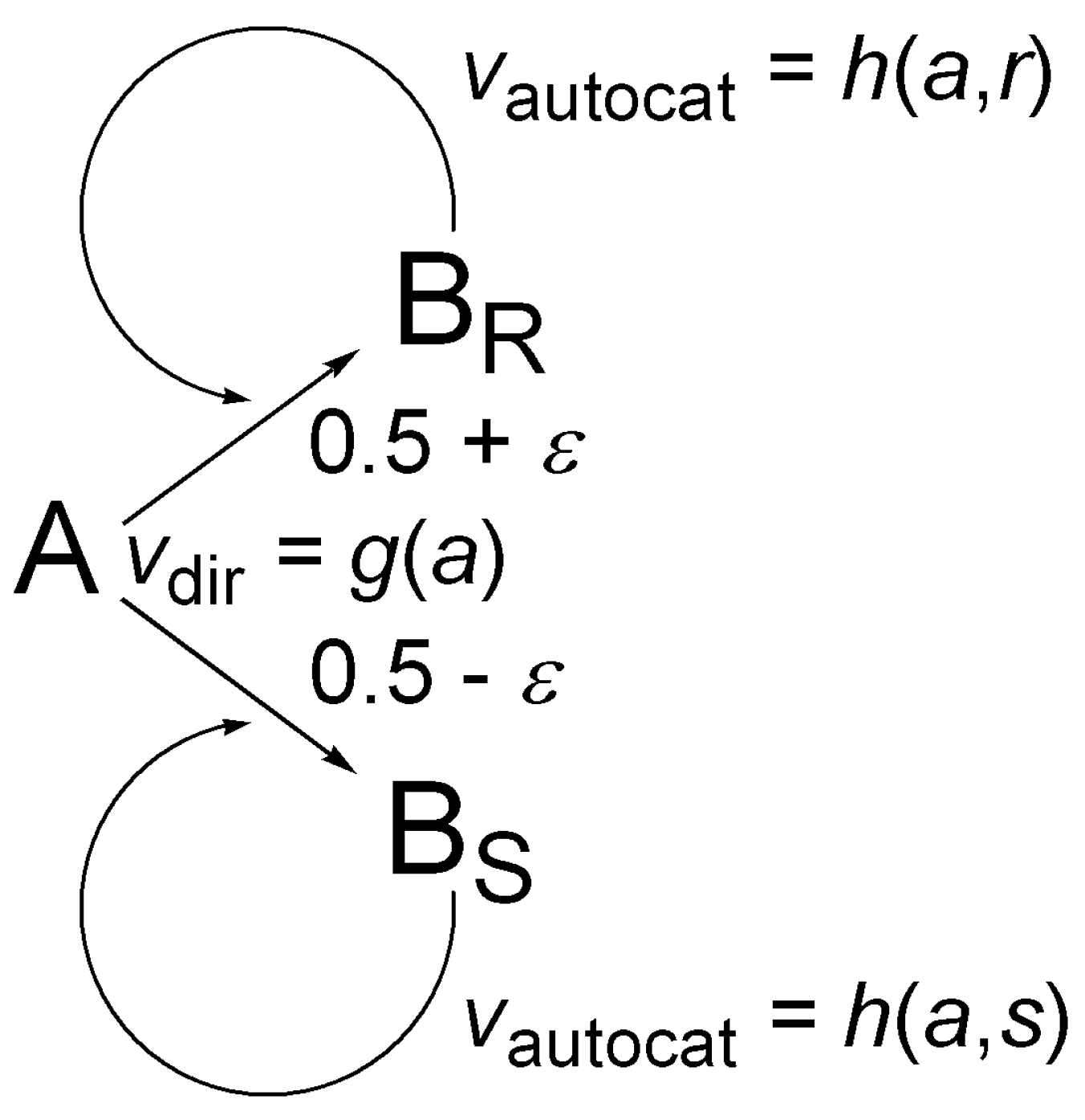
Figure 4 shows a simple chiral autocatalytic scheme where molecule A is transformed to a chiral product B, usually using some sort of reagent(s) and/or catalyst(s). This scheme has been the subject of extensive theoretical work in the last six years [35,37,38,78,79,80]. The enantiomers of B are BR and BS. Homogeneous chiral autocatalysis is represented by two parallel reactions and rate expressions shown in Figure 4: a non-catalytic direct transformation with vdir rate and an autocatalytic step with vautocat rate. Similarly to the discussion of the binomial distribution in Section 4, a small asymmetry characterized by parameter ε is considered in the direct transformation for generality.
In the mathematical discussion, a will denote the number of A molecules, r the number of BR molecules, and s the number of BS molecules present. In the rate expressions, function g(a) represents the rate of direct (not catalytic) pathway and it is only dependent on a. The scheme is also valid if the rate actually depends on additional reagents and catalysts because functions g and h only give the rate in a single kinetic run and may be different for different initial conditions, especially for different initial concentration(s) of reagent(s) and/or catalyst(s).
At t = 0, the number of A molecules present is N, the number of BR and BS molecules present is 0, etc. there is no chiral material. Conservation of mass ensures that giving only the number of BR and BS molecules is sufficient to identify any possible state of the system unambiguously: (r,s) will denote a state where the number BR molecules is exactly r, the number of BS molecules is exactly s, and consequently the number of A molecules is exactly a = N − r − s. The overall number of possible states (M) can be calculated easily:
The enumerating function, if necessary, can be given as:
The master equation of the process is the following:
The total number of B molecules, b = r + s = N − a, may also be needed for convenience in formulating certain equations. The initial state (0,0) is certain at t = 0, therefore P(0,0,0) = 1, and P(r,s,0) = 0 is valid for every other state. As explained earlier, function Q(r,s) denotes the probability that the system goes through state (r,s) at any time during the process. Q(0,0) = 1 holds because (0,0) the certain initial state. The definition equations of the expectation for xR in the final state and its standard deviation are as follows [38]:
Values of Q(r,s) can be given in a recursive formula, which shows that the final distribution only depends on the ratio of functions h and g, which will be denoted ζ(a,r) = h(a,r)/g(a).
First-order chiral autocatalysis used in a rather general sense means that the ratio of the catalytic and non-catalytic rates is directly proportional to the number of product molecules, etc. ζ(a,r) = h(a,r)/g(a) = αr irrespective of the value of a. In this case, mathematical induction based on recursive Formula 33 can be used to obtain the values of Q [38]:
The expectation for xR and its standard deviation can also be given. The first is a constant and the second only depends the value of b (= r + s) in addition to the parameters [38]:
Finally, it can be shown that the discrete distribution given in Equation 34 converges to a continuous beta distribution with parameters (0.5 + ε)α−1 and (0.5 − ε)α−1 as N approaches infinity:
For ε = 0 (no preferential isomer), Equation 37 and Equation 38 reduce to a symmetric beta distribution. Asymmetric cases of this distribution can be analyzed further by introducing new variable R to denote the probability of forming BR in excess over BS. The definition and subsequent mathematical consideration give the following formula for the general case [38]:
In Equation 39, l has the meaning that was defined in earlier Equation 20. The expectation for the enantiomeric excess in the final state can also be given:
The description of the symmetric (ε = 0) first-order autocatalytic system has been extended to initial conditions where some BR and/or BS molecules are present in the initial mixture [78] and have also been reproduced as a special case of a wider model [79]. The solution of the symmetric first-order autocatalytic system for initial conditions with non-zero BR and/or BS molecules gave the following Q function [78]:
Turning now to higher-order autocatalysis, which can be represented generally by ζ(a,r) = h(a,r)/g(a) = βjξ, the recursive definition is not easily transformed to an explicit form, but the probability of getting one enantiomer only, Q(r,0), can be given, which confirms that one of the enantiomers will be in overwhelming excess over the other for ξ > 1 and sufficiently large values of N [35,38]. However, higher-order autocatalysis in real examples does not necessarily lead to the formation enantiomeric excesses close to 100% because the convergence to the unique final distribution, unlike in the case of first-order autocatalysis, may not be very fast. For practically meaningful values of β and N, the distribution does not approach the final limit and numerical calculations are necessary, which can be based on a combined stochastic deterministic approach. First, the appropriate values of Q(r,s) are calculated with the CDS approach for a relatively small value of b0, e.g. 1,000 or 10,000 using the recursive formula given in Equation 33 in order to obtain the discrete distribution function [35]:
From the initial molar fraction of the R enantiomer (xR,i = i/b0), the expectation for the final molar fraction is calculated using the following deterministic differential Equation 35:
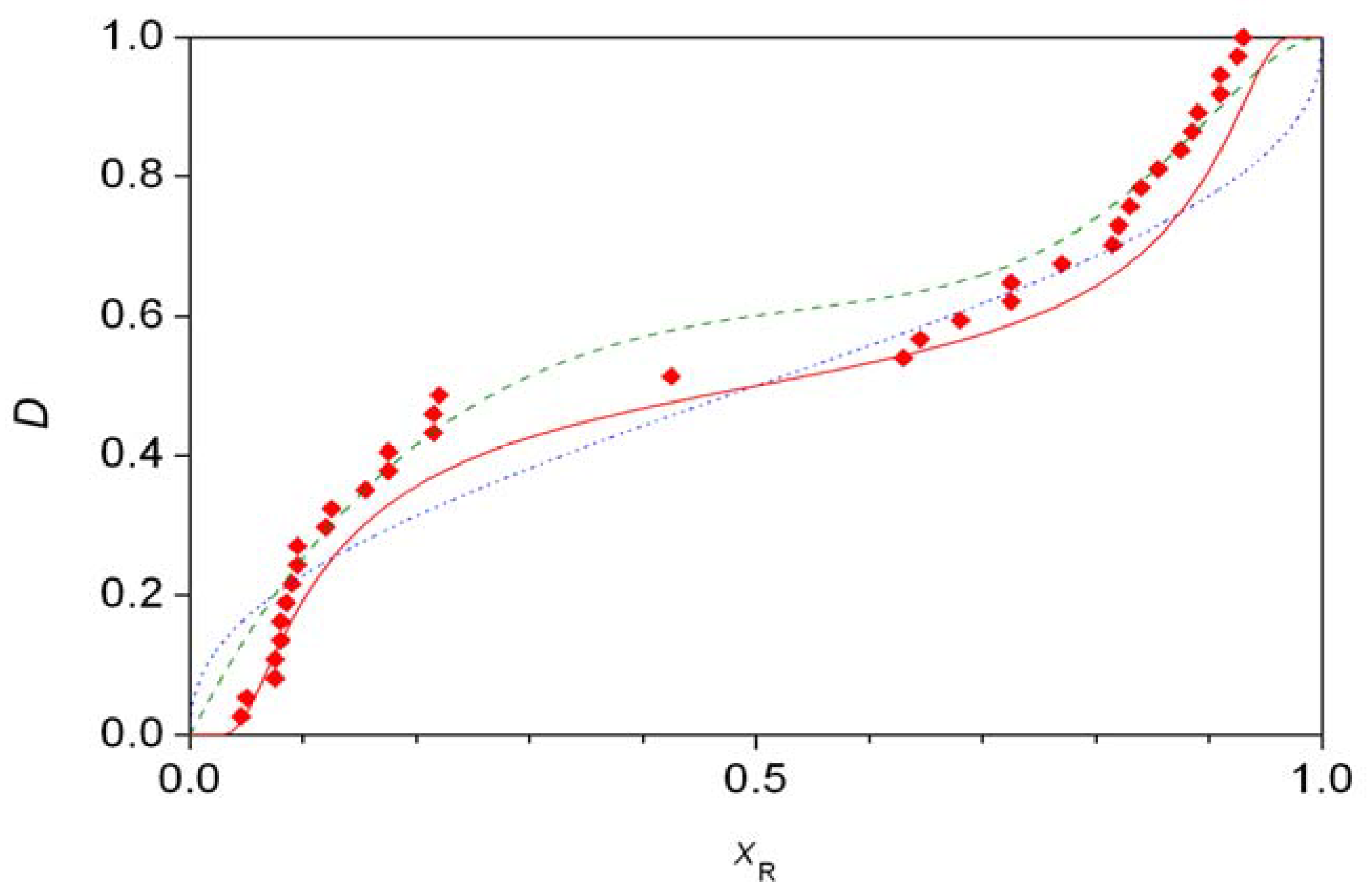
For every initial value of xR,i, numerical integration of Equation 12 between the limits b0 and N gives a final value for the molar fraction, xxR,i. The final distribution is given by F(xxrR,i). Figure 5 shows the experimental distribution of the S1 data set compared to theoretical predictions. The best fitting line (solid, red) is the one calculated assuming second-order autocatalysis [35]. The remaining two distributions shown are the one based on the best fit to first-order autocatalysis (symmetric beta distribution, blue dotted line) [37] and the combined beta distribution proposed without a model (green dashed line) in a recent work [36]. It was also pointed out that the differences in the fits are not statistically significant [35], but the primary reason for this might be the relatively low number of measured points.
Finding explicit formulas for function R and the expectation for the enantiomeric excess in the case of higher-order autocatalysis seems to be very difficult. However, the predictions of the CDS approach can still be meaningfully assessed by proving certain limiting formulas for different parameters. A higher limit can be obtained for the value of R and consequently for enantiomeric excess [38]:
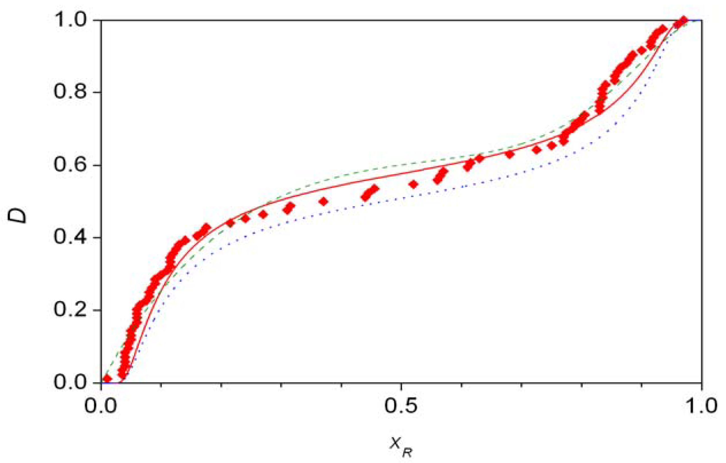
Figure 6 displays some theoretical fits to experimental distributions S2, which has been confirmed to show significant asymmetry [38,39]. The best fitting curve here is the asymmetric second-order autocatalysis (red solid line) [38], whereas the combined beta distribution (green dashed line) also gives acceptable fit but with many more parameters [36]. The final curve (blue dotted line) is the best fitting symmetric second-order autocatalytic distribution, it is shown for comparison purposes as statistic analysis clearly rejects any symmetric fit [39].
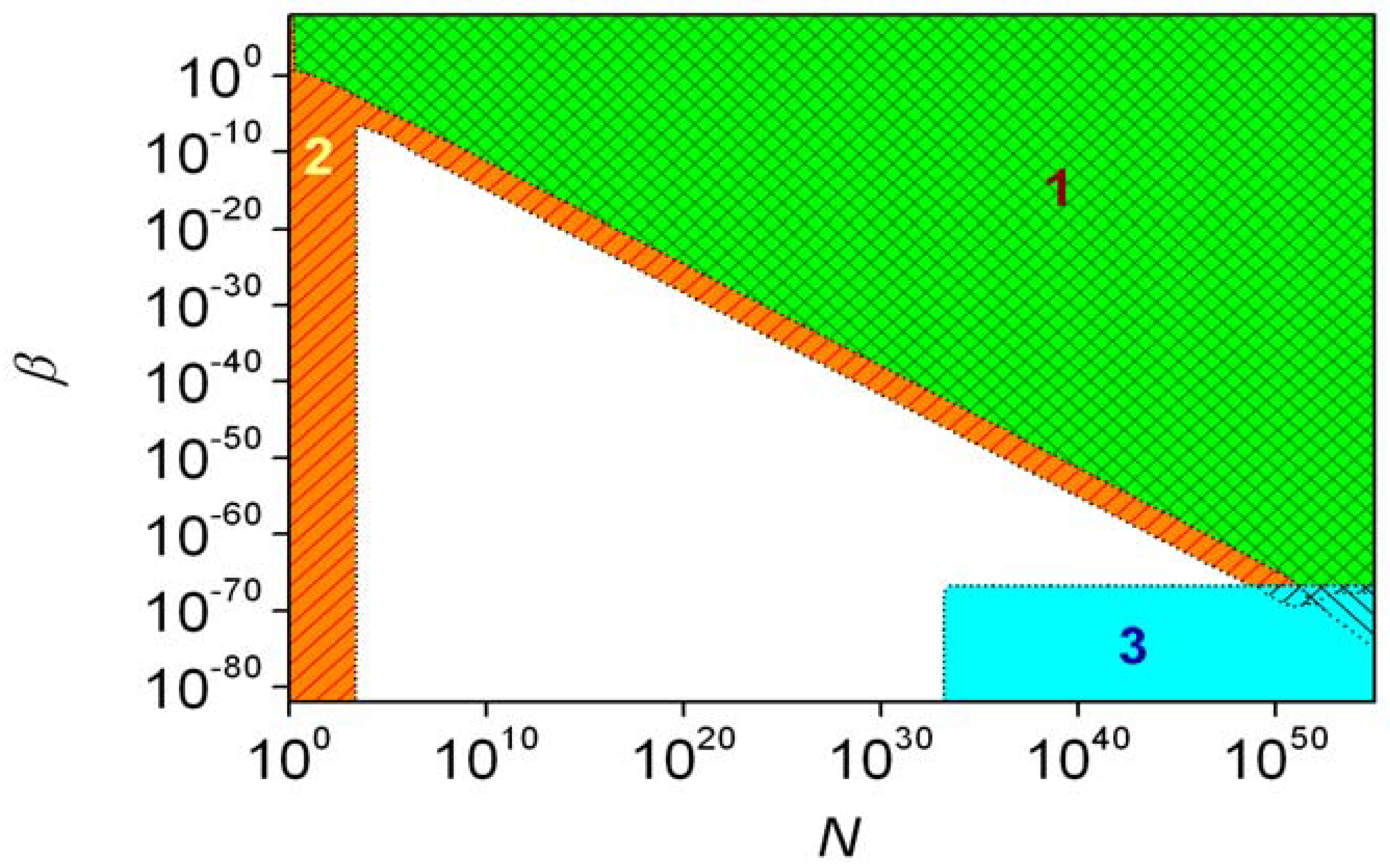
The results of the CDS approach with respect to the possibility of inherent asymmetry are best demonstrated using some arbitrarily defined conditions, which identify certain regions in the parameter space of the model [38]. When the standard deviation of the expectation of xR is larger than 0.01, conditions are said to fall into the stochastic region [38] of the model, where the final distribution of enantiomers shows average fluctuations larger than 1%. Consequently, the deterministic approach is unsuitable for describing the system.
The term de lege region [38] is only used for ε > 0 and conditions under which the probability of obtaining the BR enantiomer in excess (R) is higher than 0.9. In this region, the inherent asymmetry determines which enantiomer accumulates during amplification. The ‘significant BR excess region’ [38] is again defined for ε > 0 to denote cases where the difference between the expectation of xR and 0.5 is larger than the standard deviation of xR. This is very close to the de lege region.
Finally, the ‘high ee region’ [38] was defined as the part of the parameter space where the expectation of the enantiomeric excess formed is higher than 0.9. This is characteristically different from the de lege region, as it does not matter which of the two enantiomers is in excess.
With the estimated ε = 10−17 [54,60,61], the beta distribution is not significantly different from the one obtained with ε = 0. Therefore, the parity violating energy difference is without significant consequence in the case of first-order autocatalysis. The different regions characteristic of second-order autocatalysis (ξ = 2) are shown in Figure 7. The de lege region and the high ee region have a common area but only when the initial number if A molecules is above 1050. This is an unreasonably large number: 1050 molecules of alanine have approximately the same mass as planet Earth. It is also noticeable that the stochastic region does not contain the high ee region fully. No significant stochastic effects arise if β < 2 × 10−67, whereas a suitable N can be found within the high ee region for every value of β. It was estimated that the de lege and high ee regions cannot have common area if the initial amount of substance for reactants is smaller than 100 Gmol, no matter what the values of ξ and β are. Therefore, if present estimates [60] of the parity-violation energy difference are true, this phenomenon could have no consequence for the origin of biological chirality. Data set S2 measured in the Soai reaction gives an acceptable-looking fit to second-order autocatalysis and ε = 6.6 × 10⁻¹¹ [38], which is about seven orders of magnitude higher than could be expected based on the theoretically predicted parity violation energy difference between the enantiomers of the product of Equation 1 [61].
Some efforts have also been made to use the CDS approach to describe the stochastic phenomena in the reaction times as well. No analytical solutions were found here, but numerical studies [35] showed that even first-order autocatalysis can interpret the random fluctuations observed experimentally in the reaction between chlorite ion and iodide ion [21].
5.3. Schemes with Recycling
Saito, Sugimori, and Hyuga considered the full stochastic kinetic model based on Scheme 1 but the role of reverse reactions, called recycling, was also considered [79,80]. The deterministic equivalent of recycling was later shown to violate the second law of thermodynamics and the principle of detailed equilibrium [81,82,83]. Still, these results deserve closer attention as recent work pointed out that the mathematic equations used in recycling are identical to an open-system scenario with inflow and outflow [84].
The earlier work of Saito et al. [79] studied a scheme that can be thought of as a symmetric version of the one given in Figure 4 with h(a,r) = κ1ar + κ2ar2 but instead of g(a) implying an irreversible process, a reversible analog is used with g(a,r,s) = κ0a − λr − λs. The master equation is:
In this system, none of the states is final. Therefore, Q functions carry no meaning and the S(r,s) stationary probabilities should be defined as the final, time-independent probability values for each state:
The following formula was derived starting from master Equation 48 [79]:
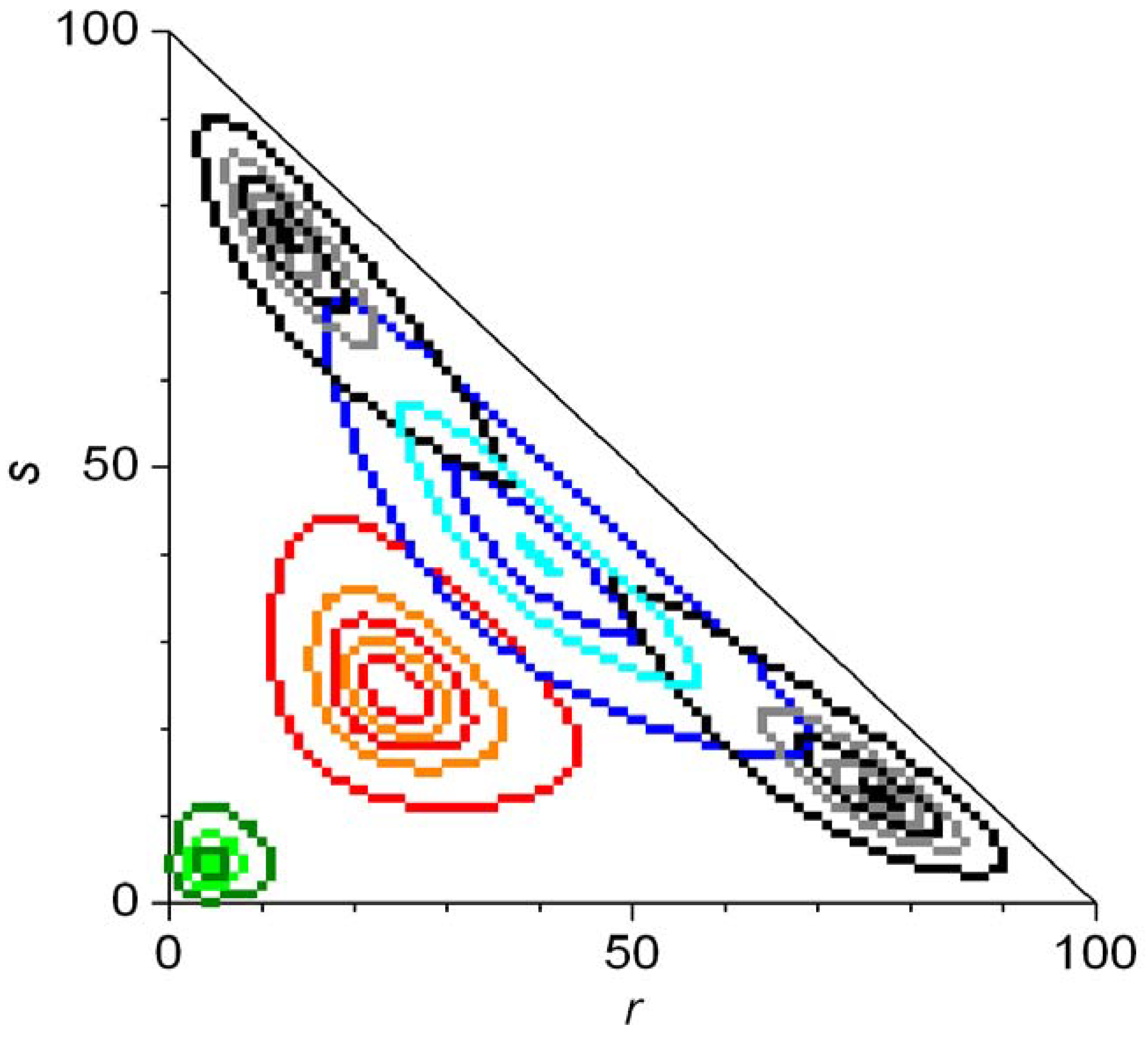
In Equation 50, Ξ is a normalizing constant and the appropriate products shown should simply be replaced by a number 1 if r = 0 or s = 0. Continuous approximations of the final distributions have also been given. Numerical integration of the master equation was carried out for N = 100 to study the evolution of the probability distribution. Figure 8 shows the evolution of the statistical distributions for the case of second order autocatalysis [79]. An eigenvalue analysis of the evolution matrix Ω was also presented [79].
Finally, this work [79] introduced a random walk approach to CDS kinetics on a square lattice (r,s) in a triangular region 0 ≤ r, s, (r + s) ≤ N for studying the system without recycling. The random walker can only make directed walks to the R and S directions: the possible steps are (r,s) → (r+1,s) and (r,s) → (r,s+1). Based on the transition probabilities in the master equation, the walker on site (r,s) stays on the site for a waiting time interval of [79]:
After the waiting time of τ, the jump is in either R or S direction with the respective probabilities of pR and pS [79]:
The essence of the random walk model and Equation 52 and Equation 53 quite analogous to the use of Q functions in some respect: the time dependence is separated from the variables of P. The recursive formula for Q values given in (33) can be thought of as a sort of random walk. The significance of this observation is that a full-scale Monte-Carlo method to the CDS approach could be based on a number of random walk procedures and used for approximating distributions of enantiomeric excesses or reaction times even if the chemical model is quite complicated and direct analytical or numerical solutions of the master equation is hindered by the very large number of states possible.
The same three authors later published a very similar analysis on a scheme which does contain any autocatalysis [80]. They showed that symmetry breaking may occur based on recycling alone. The considered reactions and rate equations are as follows:
A → BR v = κ0a
A → BS v = κ0a
R + S → 2A v = κ0rs
However, the model used contradicts the principle of microscopic reversibility [67]. A flow-through system analog [84] does not seem particularly reasonable in this case as the feed should contain a perfectly racemic mixture of BR and BS so that the ‘flow reaction’ would replace Process 54 and Process 55. Therefore, this could only be a thermodynamically acceptable model of a flow-through reactor with pre-existing chiral (but racemic) material and the reaction itself would destroy some of the chiral material to create significant enantiomeric excesses, which may not be strongly relevant for the origin of biological chirality. But again, the example showed that use of the CDS approach is necessary to understand phenomena which seem impossible within the realm of the deterministic kinetic approach.
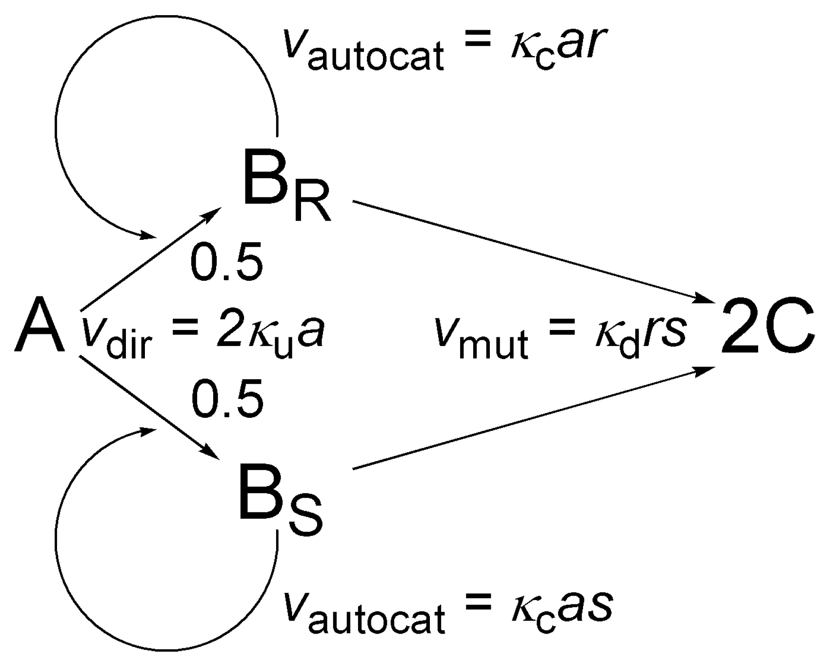
5.4. The Frank Model
Frank proposed his classic model in 1953 to give a theoretical mechanism that could lead to asymmetric synthesis [63]. This model has been the subject of more studies than can be cited here, but only a few of them had explicit stochastic elements [62,64,67,68,69,70,71,72,73,74,75,76,77,78,79,80,84]. The non-CDS studies [62,64,67,68,69,70] have already been discussed. The latest work [85] used the CDS approach primarily with numerical calculations for relatively low molecule numbers (100−1000) and without major success in finding explicit formulae for chemically more meaningful amounts of substances [85].
The model is shown in Figure 9: it basically comprises a first order version of the simple autocatalytic model shown in Figure 4 with the addition of an extra step, termed mutual antagonism by Frank [63], whereby the two enantiomers BR and BS react with each other to give nonchiral product C. Possible states can be identified by giving the numbers of molecules A (a), BR (r) and BS (s) as conservation of mass ensures c = N − a − r − s for the number of C molecules. In this system, the overall number of possible states (M) is a third-order polynomial of N:
A convenient enumerating function is:
The master equation can be written as:
Parameter κf here corresponds to the flow rate, the equation itself also describes a closed system without flow if κf = 0 is set. The expectation for enantiomeric excess in the reactor at any time is given as usual [85]:
However this traditional enantiomeric excess can be grossly misleading, as also pointed out in a deterministic analysis of closed systems [83]. Therefore, another descriptor, the yield-adjusted enantiomeric excess (E) was introduced, which is formally the product of ee and the overall yield of the chiral product [85]:
The closed system proceeds to a limited number of final states, from which no further change can arise. Obviously, Q(N,0,0) = 1 holds because (N,0,0) the certain initial state. There can be no A molecules in final states, and BR and BS molecules cannot coexist, either. The following equations have been proven [85]:
With an appropriate calculation sequence, all Q(a,r,s) values can be computed numerically conveniently for N values up to 1,000 [85]. The proved symmetries of the master equation and the solution can be used to deduce a symmetry-reduced version of the master equations, which improves the speed of computation. The master equation is homogeneous in the stochastic rate constants and, consequently, parameters can be scaled with one of the κ values with no loss of information. Figure 10 shows the probability distributions of final states calculated for N = 200 at several different κd/κu values with κc/κu = 0.01 fixed. The distribution at low κd/κu values (0.01 and lower) tends to the beta distribution given in Equation 37 and Equation 38 because the reaction responsible for mutual antagonism only occurs after all A molecules are converted to B. At higher κd/κu, the maximum at r = 0 splits into a symmetric pair, and this bimodal distribution is unchanged when κd/κu is increased above 10. At this extreme, BR or BS can only coexist for very short time periods [85].
Studying the effect of increasing the overall number of molecules revealed that there are two separate ways of increasing molecule numbers in stochastic kinetic models: at constant concentrations and increasing volume and at constant volume and increasing concentrations [85]. The first case showed the effects expected based on Kurtz’s theorem [48].
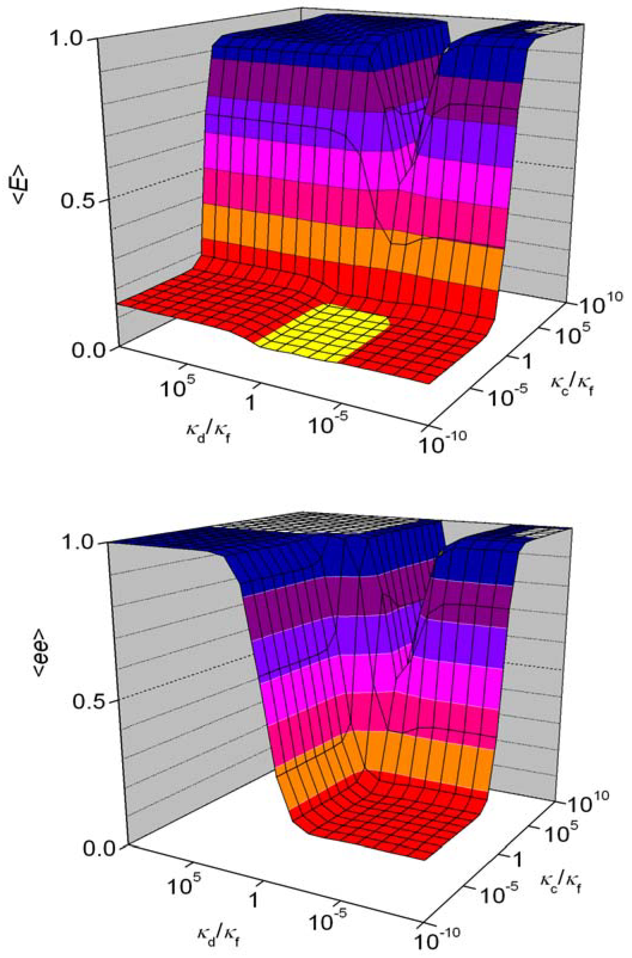
There is a substantial difference between the CDS descriptions of the Frank model in closed and flow-through systems [85]. Open-flow CDS approaches are very rare in the literature, but not without precedent [86]. The effect of flow can be thought of as a first-order process which replaces all molecules in the reactor with those in the feed [85]. In a flow-through process, there are no final states and each state can arise from or give rise to another state(s). Stationary conditions, in which none of the probabilities change any more, play a similar role in flow-through reactors as final states do in closed systems. The stationary probabilities, which are conceptually very different form the stationary concentrations used in the deterministic approach to flow-through reactors, can be calculated for all states by writing 0 on the left side of Equation 59 [85]:
In this way, the original set of M simultaneous differential equations is transformed into M homogeneous linear algebraic equations, any one of which can be obtained by summing the remaining M−1 equations. One more independent equation can be written based on the fact that all the states have been listed: the sum of all probabilities is one. These equation have a unique set of solutions, etc. the stationary probabilities are independent of initial conditions. Although the algebraic equations are linear, a special iteration method had to be developed to solve them for N = 100 (M = 176851) [85]. Further improvements in computational power are unlikely to help the numerical problems significantly, which are not primarily limited by computation time but available memory. Figure 11 shows the expectation for E and ee as a function of both κd/κf and κc/κf at fixed κu/κf and n = 100. The front left portions of both graphs provide examples when considering ee only would result in questionable conclusions. Relatively high values of κc (etc. efficient enantioselective autocatalysis) are the key to getting high E or ee values. For low values of κd (mutual antagonism), it has no influence on the course of the overall process.
An unexpected feature of Figure 11 is the ‘valley’ or ‘gorge’ at about κd/κf = 10−4 and κc/κf > 1, where intermediate values κd/κf can lead to an overall negative effect on the expectation of both E and ee because the autocatalyst is removed from the system, whereas higher κd/κf values the coexistence of BR and BS is impossible, which again favors high expectations for ee and E [85]. It was also shown that a flow-through system is not bound by Kurtz’s theorem [48].
6. Conclusions and Outlook
The resounding single conclusion of this review is that the use of stochastic models is inevitable in interpreting the origins of biological chirality. The CDS approach, used with some mathematical resourcefulness, can provide a very useful tool in interpreting absolute asymmetric reactions and the enantiomeric distributions observed in them. The CDS approach is well developed and is readily adopted for enantioselective autocatalysis, the simplest examples of which have now been studied with mathematical rigor.
The Soai reaction and other examples of absolute asymmetric synthesis have much more complex reaction mechanisms [87,88,89] than the ones studied by the CDS approach. Even with these unreasonably simple models, some success was achieved in predicting measured statistical distributions. More complex kinetic schemes, relying on the results of mechanistic studies, need to be studied in the future by the CDS approach for deeper understanding. A full-scale Monte-Carlo approach that extends the principles of the random-walk model already used in two papers [79,80] seems to have large computational potential for studying more complex reaction mechanism. In experimental work, the kinetics of the Soai reaction should be thoroughly studied under absolute asymmetric conditions and the expected random effects must be characterized.
Finally, it should also be noted that claims for thermodynamic equilibrium as a driving force of symmetry breaking exist in the relevant literature [90,91]. It is necessary to further substantiate these claims based on a stochastic approach to thermodynamics. Unlike in the case of CDS, the use of such an approach, under the name statistical thermodynamics, is often covered in detail in university physical chemistry courses and textbooks.
References and Notes
- Kennedy, D.; Norman, C. What is the origin of homochirality in nature? Science 2005, 309, 86–86. [Google Scholar]
- Progress in Biological Chirality; Pályi, G.; Zucchi, C.; Caglioti, L. (Eds.) Elsevier: Oxford, UK, 2004. [Google Scholar]
- Mislow, K. Absolute Asymmetric Synthesis: A Commentary. Collect. Czech. Chem. Commun. 2003, 68, 849–864. [Google Scholar] [CrossRef]
- Available on line: http://mathworld.wolfram.com/ (accessed on March 26, 2010).
- Soai, K.; Shibata, T.; Morioka, H.; Choji, K. Asymmetric autocatalysis and amplification of enantiomeric excess of a chiral molecule. Nature 1995, 378, 767–768. [Google Scholar] [CrossRef]
- Soai, K.; Shibata, T.; Kowata, Y. Production of Optically Active Pyrimidylalkyl Alcohol by Spontaneous Asymmetric Synthesis (in Japanese). Japan Kokai Tokkyo Koho JP 19979-268179. Application date: 1 February and 18 April, 1996.
- Soai, K.; Sato, I.; Shibata, T.; Komiya, S.; Hayashi, M.; Matsueda, Y.; Imamura, H.; Hayase, T.; Morioka, H.; Tabira, H.; Yamamoto, J.; Kowata, Y. Asymmetric synthesis of pyrimidyl alkanol without adding chiral substances by the addition of diisopropylzinc to pyrimidine-5-carbaldehyde in conjunction with asymmetric autocatalysis. Tetrahedron Asymmetry 2003, 14, 185–188. [Google Scholar] [CrossRef]
- Kawasaki, T.; Suzuki, K.; Shimizu, M.; Ishikawa, K.; Soai, K. Spontaneous absolute asymmetric synthesis in the presence of achiral silica gel in conjunction with asymmetric autocatalysis. Chirality 2006, 18, 479–482. [Google Scholar] [CrossRef] [PubMed]
- Kawasaki, T.; Shimizu, M.; Nashiyama, D.; Ito, M.; Ozawa, H.; Soai, K. Asymmetric autocatalysis induced by meteoritic amino acids with hydrogen isotope chirality. Chem. Commun. 2009, 4396–4398. [Google Scholar] [CrossRef] [PubMed]
- Kawasaki, T.; Matsamura, Y.; Tsutsumi, T.; Suzuki, K.; Ito, M.; Soai, K. Asymmetric autocatalysis triggered by carbon isotope (13C/12C) chirality. Science 2009, 324, 492–495. [Google Scholar] [CrossRef] [PubMed]
- Soai, K.; Kawasaki, T. Asymmetric autocatalysis: Automultiplication of chiral molecules. Chimica Oggi 2009, 27, 3–7. [Google Scholar]
- Gridnev, I.D.; Serafimov, J.M.; Quiney, H.; Brown, J.M. Reflections on spontaneous asymmetric synthesis by amplifying autocatalysis. Org. Biomol. Chem. 2003, 1, 3811–3819. [Google Scholar] [CrossRef]
- Singleton, D.A.; Vo, L.K. Enantioselective synthesis without discrete optically active additives. J. Am. Chem. Soc. 2002, 124, 10010–10011. [Google Scholar] [CrossRef]
- Singleton, D.A.; Vo, L.K. A few molezcules can control the enantiomeric outcome. Evidence supporting absolute asymmetric synthesis using the soai asymmetric autocatalysis. Org. Lett. 2003, 5, 4337–4339. [Google Scholar] [CrossRef] [PubMed]
- Mauksch, M.; Tsogoeva, S.B.; Wei, S.; Martynova, I.M. Demonstration of spontaneous chiral symmetry breaking in asymmetric Mannich and Aldol reactions. Chirality 2007, 19, 816–825. [Google Scholar] [CrossRef] [PubMed]
- Asakura, K.; Ikumo, A.; Kurihara, K.; Osanai, S.; Kondepudi, D.K. Random chiral asymmetry generation by chiral autocatalysis in a far-from-equilibrium reaction system. J. Phys. Chem. A 2000, 104, 2689–2694. [Google Scholar] [CrossRef]
- Asakura, K.; Osanai, S.; Kondepudi, D.K. Mechanism of chiral asymmetry generation by chiral autocatalysis in the preparation of chiral octahedral cobalt complex. Chirality 1998, 10, 343–348. [Google Scholar] [CrossRef]
- Asakura, K.; Inoue, K.; Osanai, S.; Kondepudi, D.K. Formation of the intermediate, aquohydroxobis(ethylenediamine)cobalt(II) complex, in the preparation of cis-bromoamminebis-(ethylenediamine)cobalt(III) bromide by the reaction of bis[bis(ethylenediamine)cobalt(III)-μ-dihydroxo]diaquocobalt(II) sulfate with ammonium bromide in water. J. Coord. Chem. 1998, 46, 159–164. [Google Scholar]
- Asakura, K.; Osanai, S.; Kondepudi, D.K. Conditions for chiral asymmetry generation in the preparation of the chiral octahedral cobalt complex. Chirality 2001, 13, 435–440. [Google Scholar] [CrossRef]
- Nagypál, I.; Epstein, I.R. Fluctuations and stirring rate effects in the chlorite-thiosulfate reaction. J. Phys. Chem. 1986, 90, 6285–6292. [Google Scholar] [CrossRef]
- Nagypál, I.; Epstein, I.R. Stochastic behavior and stirring rate effects in the chlorite-iodide Reaction. J. Chem. Phys. 1988, 89, 6925–6928. [Google Scholar] [CrossRef]
- Lente, G.; Fábián, I.; Bazsa, G. What is and what isn’t a clock reaction? New J. Chem. 2007, 31, 1707. [Google Scholar] [CrossRef]
- Pasteur, L. Research on the relationship between crystalline form, chemical composition, and the sense of rotatory polarization (in French). Ann. Chem. Phys. (3rd Ser.) 1848, 24, 442–459. [Google Scholar]
- Gal, J. The Discovery of Biological Enantioselectivity: Louis Pasteur and the Fermentation of Tartaric Acid, 1857-A Review and Analysis 150 Year Later. Chirality 2008, 20, 5–19. [Google Scholar] [CrossRef] [PubMed]
- Kondepudi, D.K.; Kaufman, R.J.; Singh, N. Chiral symmetry breaking in sodium chlorate crystallization. Science 1990, 250, 975–976. [Google Scholar] [CrossRef] [PubMed]
- Kondepudi, D.K.; Culha, M. Chiral interaction and stochastic kinetics in stirred crystallization of amino acids. Chirality 1998, 10, 238–245. [Google Scholar] [CrossRef]
- Kondepudi, D.K.; Asakura, K. Chiral autocatalysis, spontaneous symmetry breaking, and stochastic behavior. Acc. Chem. Res. 2001, 34, 946–954. [Google Scholar] [CrossRef] [PubMed]
- Matsuura, T.; Koshima, H. Introduction to chiral crystallization of achiral organic compounds. Spontaneous generation of chirality. J. Photochem. Photobiol. C Photochem. Rev. 2005, 6, 7–24. [Google Scholar] [CrossRef]
- Viedma, C. Chiral Symmetry Breaking During Crystallization: Complete Chiral Purity Induced by Nonlinear Autocatalysis and Recycling. Phys. Rev. Lett. 2005, 94, 065504:1–065504:4. [Google Scholar] [CrossRef] [PubMed]
- Gridnev, I.D. Chiral symmetry breaking in chiral crystallization and soai autocatalytic reaction. Chem. Lett. 2006, 35, 148–153. [Google Scholar] [CrossRef]
- Pérez-García, L.; David, B.; Amabilino, D.B. Spontaneous Resolution, Whence and Whither: From Enantiomorphic Solids to Chiral Liquid Crystals, Monolayers and Macro- and Supra-Molecular Polymers and Assemblies. Chem. Soc. Rev. 2007, 36, 941–967. [Google Scholar] [CrossRef]
- McBride, J.M.; Tully, J.C. Did life grind to a start? Nature 2008, 452, 161–162. [Google Scholar] [CrossRef]
- Blackmond, D.G.; Klussmann, M. Spoilt for Choice: Assessing Phase Behavior Models for the Evolution of Homochirality. Chem. Commun. 2007, 3990–3996. [Google Scholar] [CrossRef]
- Tamura, R.; Iwama, S.; Takahashi, H. Chiral symmetry breaking phenomenon caused by a phase transition. Symmetry 2010, 2, 112–135. [Google Scholar] [CrossRef]
- Lente, G. Stochastic Kinetic Models of Chiral Autocatalysis: A General Tool for the Quantitative Interpretation of Total Asymmetric Synthesis. J. Phys. Chem. A 2005, 109, 11058–11063. [Google Scholar] [CrossRef] [PubMed]
- Barabás, B.; Caglioti, L.; Micskei, K.; Pályi, G. Data-based stochastic approach to absolute asymmetric synthesis by autocatalysis. Bull. Chem. Soc. Jpn. 2009, 82, 1372–1376. [Google Scholar] [CrossRef]
- Lente, G. Homogeneous Chiral Autocatalysis: A Simple, Purely Stochastic Kinetic Model. J. Phys. Chem. A 2004, 108, 9475–9478. [Google Scholar] [CrossRef]
- Lente, G. The effect of parity violation on kinetic models of enantioselective autocatalysis. Phys. Chem. Chem. Phys. 2007, 9, 6134–6141. [Google Scholar] [CrossRef] [PubMed]
- Barabás, B.; Caglioti, L.; Zucchi, C.; Maioli, M.; Gál, E.; Micskei, K.; Pályi, G. Violation of distribution symmetry in statistical evaluation of absolute enantioselective synthesis. J. Phys. Chem. B 2007, 111, 11506–11510. [Google Scholar] [CrossRef] [PubMed]
- Caglioti, L.; Barabás, B.; Faglioni, F.; Florini, N.; Lazzeretti, P.; Maioli, M.; Micskei, K.; Rábai, G.; Taddei, F.; Zucchi, C.; Pályi, G. On the track of absolute enantioselective catalysis. Chimica Oggi 2008, 26, 30–32. [Google Scholar]
- Barabás, B.; Caglioti, L.; Faglioni, F.; Florini, N.; Lazzaretti, P.; Maioli, M.; Micskei, K.; Rabai, G.; Taddei, F.; Zucchi, C.; Pályi, G. On the traces of absolute enantioselective synthesis. AIP Conf. Proc. 2008, 963B, 1150–1152. [Google Scholar]
- Delbrück, M. Statistical fluctuation in autocatalytic reactions. J. Chem. Phys. 1940, 8, 120. [Google Scholar] [CrossRef]
- Érdi, P.; Tóth, J. Stochastic reaction kinetics = "nonequilibrium thermodynamics" of the state space? React. Kinet. Catal. Lett. 1976, 4, 81–85. [Google Scholar] [CrossRef]
- Érdi, P.; Tóth, J. Mathematical Models of Chemical Reactions; Manchester University Press: Manchester, UK, 1989; pp. 91–161. [Google Scholar]
- de Marcillac, P.; Coron, N.; Dambier, G.; Leblanc, J.; Moalic, J.P. Experimental detection of α-particles from the radioactive decay of natural bismuth. Nature 2003, 422, 876–878. [Google Scholar] [CrossRef] [PubMed]
- Yukalov, V.I. Systems with symmetry breaking and restoration. Symmetry 2010, 2, 40–68. [Google Scholar] [CrossRef]
- Singer, K. Application of the theory of stochastic processes to the study of irreproducible chemical reactions and nucleation processes. J. Roy. Stat. Soc. Ser. B. 1953, 15, 92–106. [Google Scholar] [CrossRef]
- Kurtz, T.G. The relationship between stochastic and deterministic models for chemical reactions. J. Chem. Phys. 1972, 57, 2976–2978. [Google Scholar] [CrossRef]
- Mills, W. Some aspects of stereochemistry. Chem. Ind. (London) 1932, 51, 750–759. [Google Scholar] [CrossRef]
- Siegert, A.J.F. On the approach to statistical equilibrium. Phys. Rev. 1949, 76, 1708–1714. [Google Scholar] [CrossRef]
- Caglioti, L.; Zucchi, C.; Pályi, G. Single-molecule chirality. Chimica Oggi 2005, 23, 38–43. [Google Scholar]
- Weissbuch, I.; Leiserowitz, L.; Lahav, M. Stochastic “Mirror Symmetry Breaking” via Self-Assembly, Reactivity and Amplification of Chirality: Relevance to Abiotic Conditions. Top. Curr. Chem. 2005, 259, 123–165. [Google Scholar]
- Pályi, G.; Micskei, K.; Zékány, L.; Zucchi, C.; Caglioti, L. Racemates and the soai reaction (in Hungarian). Magyar Kém. Lapja 2005, 60, 17–24. [Google Scholar]
- Lente, G. Stochastic analysis of the parity-violating energy differences between enantiomers and its implications for the origin of biological chirality. J. Phys. Chem. A 2006, 110, 12711–12713. [Google Scholar] [CrossRef]
- Caglioti, L.; Hajdu, C.; Holczknecht, O.; Zékány, L.; Zucchi, C.; Micskei, K.; Pályi, G. The concept of racemates and the soai-reaction. Viva Origino 2006, 34, 62–80. [Google Scholar]
- Caglioti, L.; Pályi, G. Chiral chemistry of single molecules. Chimica Oggi 2008, 26, 41–42. [Google Scholar]
- Barabás, B.; Caglioti, L.; Micskei, K.; Zucchi, C.; Pályi, G. Isotope Chirality and Asymmetric Autocatalysis: A Possible Entry to Biological Chirality. Orig. Life Evol. Biosph. 2008, 38, 317–327. [Google Scholar]
- Fuß, W. Does life originate from a single molecule? Chirality 2009, 21, 299–304. [Google Scholar] [CrossRef] [PubMed]
- Fuß, W. Biological homochirality as result from a single event. Coll. Surf. B: Biointerf. 2009, 74, 498–503. [Google Scholar] [CrossRef] [PubMed]
- Quack, M. How important is parity violation for molecular and biomolecular chirality? Angew. Chem. Int. Ed. 2002, 41, 4619–4630. [Google Scholar] [CrossRef] [PubMed]
- Faglioni, F.; Lazzeretti, P.; Pályi, G. Parity violation energy of 5-pyrimidyl alkanol, a chiral autocatalytic molecule. Chem. Phys. Lett. 2007, 435, 346–349. [Google Scholar] [CrossRef]
- Todorović, D.; Gutman, I.; Radulović, M. A stochastic chiral amplification model. Chem. Phys. Lett. 2003, 372, 464–468. [Google Scholar] [CrossRef]
- Frank, F.C. On spontaneous asymmetric synthesis. Biochim. Biophys. Acta 1953, 11, 459–463. [Google Scholar] [CrossRef]
- Cruz, J.M.; Parmananda, P.; Buhse, T. Noise-induced enantioselection in chiral autocatalysis. J. Phys. Chem. A 2008, 112, 1673–1676. [Google Scholar] [CrossRef] [PubMed]
- Rivera Islas, J.; Lavabre, D.; Jean-Michel Grevy, J.M.; Hernández Lamoneda, R.; Rojas Cabrera, H.; Micheau, J.C.; Buhse, T. Mirror-Symmetry Breaking in the Soai Reaction: A Kinetic Understanding. Proc. Natl. Acad. Sci. USA 2005, 101, 5732–5736. [Google Scholar]
- Micskei, K.; Rábai, G.; Gál, E.; Caglioti, L.; Pályi, G. Oscillatory symmetry breaking in the soai reaction. J. Phys. Chem. B 2008, 112, 9196–9200. [Google Scholar] [CrossRef] [PubMed]
- Hochberg, D.; Zorzano, M.P. Reaction-noise induced homochirality. Chem Phys. Lett. 2006, 431, 185–189. [Google Scholar] [CrossRef]
- Hochberg, D.; Zorzano, M.P. Mirror symmetry breaking as a problem in dynamic critical phenomena. Phys. Rev. E 2007, 76, 021109:1–021109:8. [Google Scholar] [CrossRef] [PubMed]
- Hochberg, D. Mirror Symmetry Breaking and Restoration: The Role of Noise and Chiral Bias. Phys. Rev. Lett. 2009, 102, 248101:1–248101:4. [Google Scholar] [CrossRef] [PubMed]
- Hochberg, D. Effective potential and chiral symmetry breaking. Phys. Rev E 2010, 81, 016106:1–016106:13. [Google Scholar] [CrossRef] [PubMed]
- Gleiser, M.; Walker, S.I. An Extended Model for the Evolution of Prebiotic Homochirality: A Bottom-Up Approach to the Origin of Life. Orig. Life Evol. Biosph. 2008, 38, 293–315. [Google Scholar] [CrossRef] [PubMed]
- Gillespie, D.T. Deterministic limit of stochastic chemical kinetics. J. Phys. Chem. B 2009, 113, 1640–1644. [Google Scholar] [CrossRef] [PubMed]
- Bartholomay, A.F. A stochastic approach to statistical kinetics with application to enzyme kinetics. Biochem. 1962, 1, 223–230. [Google Scholar] [CrossRef]
- Arányi, P.; Tóth, J. A full stochastic description of the Michaelis-Menten reaction for small systems. Acta Biochim. Biophys. Acad. Sci. Hung. 1977, 12, 375–388. [Google Scholar]
- Kou, S.C.; Cherayil, B.J.; Min, W.; English, B.P.; Xie, X.S. Single-molecule michaelis-menten equations. J. Phys. Chem. B 2005, 109, 19068–19081. [Google Scholar] [CrossRef] [PubMed]
- Velonia, K.; Flomenbom, O.; Loos, D.; Masuo, S.; Cotlet, M.; Engelborghs, Y.; Hofkens, J.; Rowan, A.E.; Klafter, J.; Nolte, R.J.M.; de Schryver, F.C. Single-enzyme kinetics of CALB-catalyzed hydrolysis. Angew. Chem. Int. Ed. 2005, 44, 560–564. [Google Scholar] [CrossRef] [PubMed]
- Choi, P.J.; Cai, L.; Frieda, K.; Xie, X.S. A stochastic single-molecule event triggers phenotype switching of a bacterial cell. Science 2008, 322, 442–446. [Google Scholar] [CrossRef] [PubMed]
- Shao, J.; Liu, L. Stochastic Fluctuations and Chiral Symmetry Breaking: Exact Solution of Lente Model. J. Phys. Chem. A 2007, 111, 9570–9572. [Google Scholar] [CrossRef] [PubMed]
- Saito, Y.; Sugimori, T.; Hyuga, H. Stochastic approach to enantiomeric excess amplification and chiral symmetry breaking. J. Phys. Soc. Japan 2007, 76, 044802:1–044802:14. [Google Scholar] [CrossRef]
- Sugimori, T.; Hyuga, H.; Saito, Y. Fluctuation induced homochirality. J. Phys. Soc. Japan 2008, 77, 064606:1–064606:6. [Google Scholar] [CrossRef]
- Blackmond, D.G.; Matar, O.K. Re-examination of reversibility in reaction models for the spontaneous emergence of homochirality. J. Phys. Chem. B 2008, 112, 5098–5104. [Google Scholar] [CrossRef]
- Lente, G. Theromdynamic unfeasibility of recycling in chiral autocatalytic kinetic models. React. Kinet. Catal. Lett. 2008, 95, 13–19. [Google Scholar] [CrossRef]
- Blackmond, D.G. “If Pigs Could Fly” Chemistry: A Tutorial on the Principle of Microscopic Reversibility. Angew. Chem. Int. Ed. 2009, 48, 2648–2654. [Google Scholar] [CrossRef]
- Lente, G. Open system approaches in deterministic models of the emergence of homochirality. Chirality 2010, 22. [Google Scholar] [CrossRef]
- Lente, G.; Ditrói, T. Stochastic kinetic analysis of the frank model. Stochastic approach to flow-through reactors. J. Phys. Chem. A 2009, 113, 7237–7242. [Google Scholar] [CrossRef] [PubMed]
- Ishida, K. Stochastic Approach to nonequilibrium thermodynamics of first-order chemical reactions. II. Open systems. J. Phys. Chem. 1968, 72, 92–96. [Google Scholar] [CrossRef]
- Buhse, T. A tentative kinetic model for chiral amplification in autocatalytic alkylzinc additions. Tetrahedron Asymmetry 2003, 14, 1055–1061. [Google Scholar] [CrossRef]
- Lavabre, D.; Micheau, J.C.; Rivera Islas, J.; Buhse, T. Mirror-symmetry breaking in the Soai reaction: A kinetic understanding. J. Phys. Chem. A 2007, 111, 281–286. [Google Scholar] [CrossRef] [PubMed]
- Schiaffino, L.; Ercolani, G. Unraveling the Mechanism of the Soai Asymmetric Autocatalytic Reaction by First-Principles Calculations: Induction and Amplification of Chirality by Self-assembly of Hexanuclear Complexes. Angew. Chem. Int. Ed. 2008, 47, 6832–6835. [Google Scholar] [CrossRef] [PubMed]
- Crusats, J.; Veintemillas-Verdaguer, S.; Ribó, J.M. Homochirality as a consequence of thermodynamic equilibrium? Chem. Eur. J. 2006, 12, 7576–7581. [Google Scholar] [CrossRef] [PubMed]
- Klussmann, M.; Iwamura, H.; Mathew, S.P.; Wells, D.H., Jr.; Pandya, U.; Armstrong, A.; Blackmond, D.G. Thermodynamic control of asymmetric amplification in amino acid catalysis. Nature 2006, 441, 621–623. [Google Scholar] [CrossRef]
Scheme 1.
The Soai reaction.

Figure 1.
Statistical enantiomeric excess distributions (D: distribution function) measured in various absolute asymmetric reactions. Origin of data: Reference [7] (S1); Reference [8] (S2); Reference [12] (G); Reference [16] (A).

Scheme 2.
Absolute asymmetric Mannich and aldol reactions.

Scheme 3.
Absolute asymmetric cleavage of a trinuclear cobalt complex.

Figure 2.
Statistical reaction time distributions (D: distribution function) measured in the chlorite ion–thiosulfate ion (N1) [20] and chlorite ion–iodide ion (N2) [21] reaction.

Figure 3.
Probability of obtaining the favored enantiomer in excess in the case of asymmetric binomial distribution [54].
Figure 3.
Probability of obtaining the favored enantiomer in excess in the case of asymmetric binomial distribution [54].

Figure 4.
General symmetry breaking model with enantioselective autocatalysis.

Figure 5.
Fit of different theoretical distributions (D: distribution function) to data set S1. Solid red line: second-order autocatalysis [35], blue dotted line: first-order autocatalysis [37], green dashed line: combined beta distribution [36].

Figure 6.
Fit of different theoretical distributions (D: distribution function) to data set S2. Solid red line: second-order autocatalysis with a favored isomer [38], blue dotted line: second-order autocatalysis without a favored isomer [35], green dashed line: combined beta distribution [36].

Figure 7.
Different regions in the parameter space for second-order autocatalysis as a function of parameters N and β [38]. (1: high ee region, 2: stochastic region, 3: de lege region).
Figure 7.
Different regions in the parameter space for second-order autocatalysis as a function of parameters N and β [38]. (1: high ee region, 2: stochastic region, 3: de lege region).

Figure 8.
Contour plot of the time evolution of statistical distributions in a scheme with second-order autocatalysis and recycling [79]. Parameters: κ2 = 0.001 × κ0, λ = κ0, N = 100, tκ0 = 0.0536 (green), 0.3362 (red), 0.7915 (blue), ∞ (black).
Figure 8.
Contour plot of the time evolution of statistical distributions in a scheme with second-order autocatalysis and recycling [79]. Parameters: κ2 = 0.001 × κ0, λ = κ0, N = 100, tκ0 = 0.0536 (green), 0.3362 (red), 0.7915 (blue), ∞ (black).

Figure 9.
The Frank model.

Figure 10.
Final probability distributions in the Frank model in a closed system at κc/κu = 0.01. Numbers displayed inside the graph show the value of κd/κu for each distribution shown [85].
Figure 10.
Final probability distributions in the Frank model in a closed system at κc/κu = 0.01. Numbers displayed inside the graph show the value of κd/κu for each distribution shown [85].

Figure 11.
Expectation of the yield-adjusted and conventional enantiomeric excess for the Frank model in an open system with κu/κf = 1 and N = 100 [85].
Figure 11.
Expectation of the yield-adjusted and conventional enantiomeric excess for the Frank model in an open system with κu/κf = 1 and N = 100 [85].

© 2010 by the author; licensee Molecular Diversity Preservation International, Basel, Switzerland. This article is an open-access article distributed under the terms and conditions of the Creative Commons Attribution license (http://creativecommons.org/licenses/by/3.0/).
Share and Cite
MDPI and ACS Style
Lente, G. The Role of Stochastic Models in Interpreting the Origins of Biological Chirality. Symmetry 2010, 2, 767-798. https://doi.org/10.3390/sym2020767
AMA Style
Lente G. The Role of Stochastic Models in Interpreting the Origins of Biological Chirality. Symmetry. 2010; 2(2):767-798. https://doi.org/10.3390/sym2020767
Chicago/Turabian StyleLente, Gábor. 2010. "The Role of Stochastic Models in Interpreting the Origins of Biological Chirality" Symmetry 2, no. 2: 767-798. https://doi.org/10.3390/sym2020767