New Chaotic Systems with Two Closed Curve Equilibrium Passing the Same Point: Chaotic Behavior, Bifurcations, and Synchronization

Abstract

In this work, we introduce a chaotic system with infinitely many equilibrium points laying on two closed curves passing the same point. The proposed system belongs to a class of systems with hidden attractors. The dynamical properties of the new system were investigated by means of phase portraits, equilibrium points, Poincaré section, bifurcation diagram, Kaplan–Yorke dimension, and Maximal Lyapunov exponents. The anti-synchronization of systems was obtained using the active control. This study broadens the current knowledge of systems with infinite equilibria.

1. Introduction

Chaotic systems have been widely studied and used in various practical fields by mathematicians, physicists, scientists, and engineers in the past four decades; see [1,2,3,4] and the references therein. Many chaotic systems with different shapes of attractors have been reported, such as chaotic systems with butterfly attractors (see, e.g., [5]) and systems with multiscroll chaotic attractors (see, e.g., [6]). Recent developments include some different types of chaotic systems with no equilibrium points (see, e.g., [7]), with a single stable equilibrium (see, e.g., [8]), with a line of equilibrium points (see, e.g., [9]), with a circular equilibrium (see, e.g., [10]), with circle and square equilibrium (see, e.g., [11]), with rounded square loop equilibrium (see, e.g., [12]), and with different closed curve equilibrium (see, e.g., [13]). Furthermore, it has also been applied in many different areas including information processing (see, e.g., [14]) and chaotic masking communication (see, e.g., [15]).

According to a new classification of chaotic dynamics [16], there are two kinds of attractors: self-excited attractors and hidden attractors. Recall that an attractor is referred to as being $\mathit{self-excited}$ if its basin of attraction intersects any arbitrarily small open neighborhood of an equilibrium, otherwise it is called a $\mathit{hidden}$. The basin of attraction for a hidden attractor is not connected with any unstable fixed point. For example, hidden attractors are observed in the systems without fixed points, with no unstable fixed points, or with one stable fixed point. A system with infinitely many equilibrium points can be classified as one system with hidden attractors, for the reason that we do not know which part of the equilibria may be used to localize the hidden attractors, which should be treated in detail (see, e.g., [17]). Recent important investigations and developments in the study of chaotic dynamical systems with practical problems and challenges have been asked to satisfy at least one of the following criteria as Sprott mentioned in [18]: (S1) The system should credibly model some important unsolved problem in nature and shed light on that problem; (S2) the system should exhibit some behavior previously unobserved; (S3) the system should be simpler than all other known examples exhibiting the observed behavior. An important ongoing research topic is dedicated to discovering and developing new and novel chaotic systems with different shapes of closed curve equilibrium.

The main goal of this work is to present a new system with infinitely many equilibrium points arranged on two closed curves passing the same point, which extends the general knowledge about such systems. Our new chaotic system (see Section 2 below for details) is meaningful for satisfying two of the three conditions, (S1), (S2), and (S3), as well as there being a certain novelty value in this work. In Section 2, some dynamical properties of the proposed system, which have been studied using a bifurcation diagram, phase portrait, Poincaré section, maximal Lyapunov exponents, and Kaplan–Yorke dimension, are presented. The ability of anti-synchronization of the new system is also discussed in Section 3.

2. A New Family with Two Closed Curve Equilibrium

In this work, motivated by the known dynamic systems mentioned above, we study the following general model given by

$$\begin{array}{cc}\hfill \dot{u}& =w,\hfill \\ \hfill \dot{v}& =-wf(u,v,w),\hfill \\ \hfill \dot{w}& =g(u,v),\hfill \end{array}$$

(1)

where u, v and w are three state variables, $f(u,v,w)$ and $g(u,v)$ are two nonlinear functions. The equilibrium points in model (1) can be obtained by calculating

$$\begin{array}{cc}\hfill w& =0,\hfill \\ \hfill -wf(u,v,w)& =0,\hfill \\ \hfill g(u,v)& =0.\hfill \end{array}$$

(2)

It is obtained that the equilibrium points locate on a curve described by $g(u,v)=0$ in the plane $w=0$. In fact, by selecting appropriate functions f and g, some known systems, both chaotic and with different closed curve equilibrium, can be constructed.

$(Example$ $A)$

Take $f(u,v,w)=\alpha v+\beta v^2+uw$ and $g(u,v)=u^2+v^2-1$, then model (1) will deduce the following system

$$\begin{array}{cc}\hfill \dot{u}& =w,\hfill \\ \hfill \dot{v}& =-w(\alpha v+\beta v^2+uw),\hfill \\ \hfill \dot{w}& =u^2+v^2-1,\hfill \end{array}$$

(3)

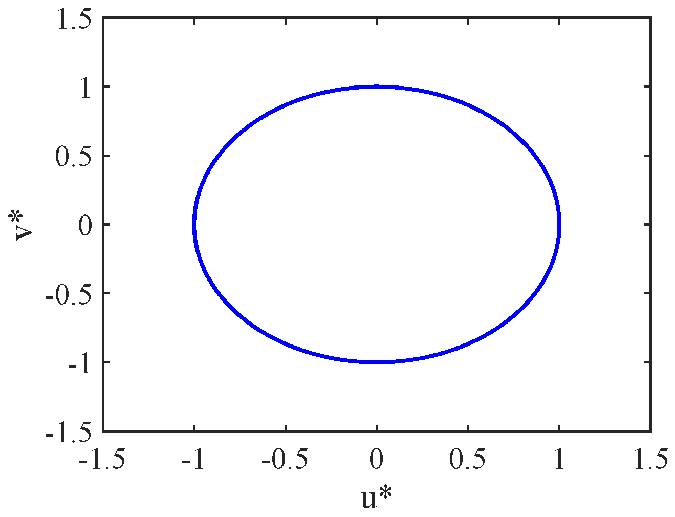
which was introduced and studied by Gotthans, Sprott, and Petrzela [11] in 2016. The chaotic systems (3) has circle equilibrium (see Figure 1).

$(Example$ $B)$

Let $f(u,v,w)=\alpha v+\beta v^2+uw$ and $g(u,v)=u^2-\left|uv\right|+v^2-1$. Then, model (1) deduces the following system:

$$\begin{array}{cc}\hfill \dot{u}& =w,\hfill \\ \hfill \dot{v}& =-w(\alpha v+\beta v^2+uw),\hfill \\ \hfill \dot{w}& =u^2-\left|uv\right|+v^2-1,\hfill \end{array}$$

(4)

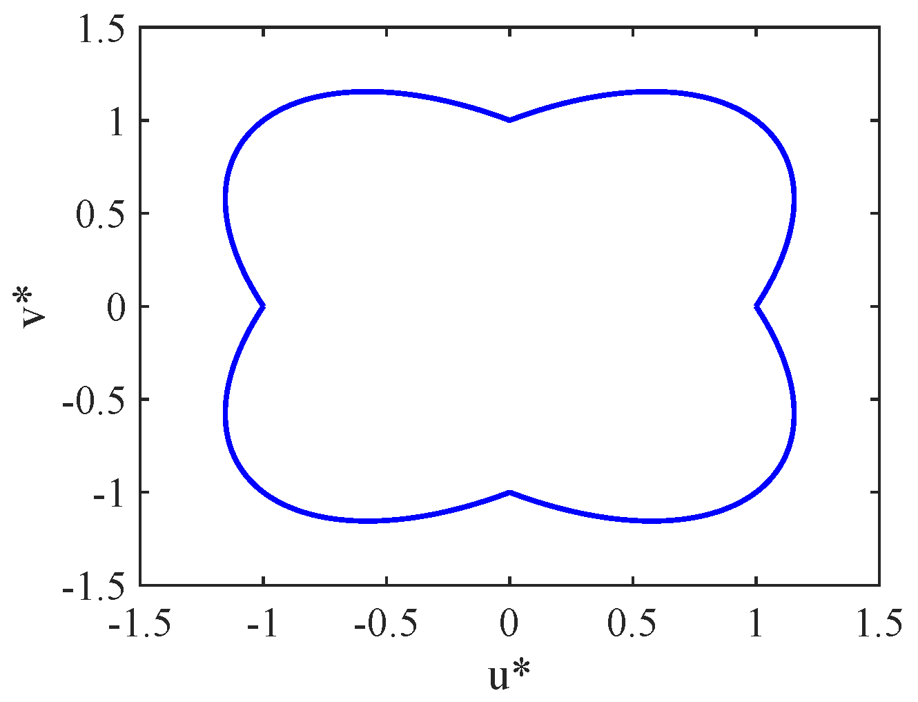
which was established by Wang, Pham, and Volos [19] in 2017. The chaotic system (4) has cloud-shaped curve equilibrium, as shown in Figure 2.

$(Example$ $C)$

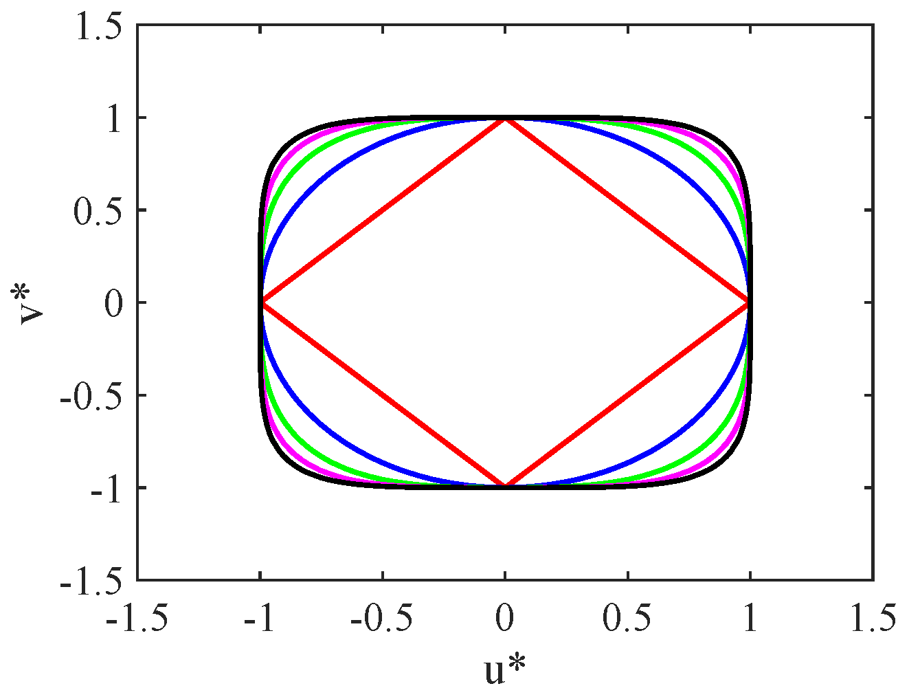
Very recently, Zhu and Du [13] discovered and studied a new family of systems with different equilibrium (as shown in Figure 3) described by

$$\begin{array}{cc}\hfill \dot{u}& =w,\hfill \\ \hfill \dot{v}& =-w(\alpha v+\beta v^2+uw),\hfill \\ \hfill \dot{w}& ={\left|u\right|}^k+{\left|v\right|}^k-1,\hfill \end{array}$$

(5)

where $k\in$ $\mathbb{N}$. In fact, the chaotic system (5) can be obtained by putting $f(u,v,w)=\alpha v+\beta v^2+uw$ and $g(u,v)={\left|u\right|}^k+{\left|v\right|}^k-1$ into model (1). In [13], Zhu and Du analyzed the dynamical properties of their proposed systems using the methods of equilibrium points, eigenvalues, phase portraits, maximal Lyapunov exponents, and Kaplan–Yorke dimension; see [13] for more details.

The results established in [11,13,19] are very important for indicating the existence of chaotic systems with different shapes of equilibrium points (see

Table 1. Chaotic systems with infinitely many equilibrium points.

System	Equilibrium	Closed Curve Equilibrium	Paper
Gotthans, Sprott, and Petrzela	$u^2+v^2-1=0$	Circle	[11]
Zhu and Du	${\left|u\right|}^k+{\left|v\right|}^k-1=0$	Circle, Square, etc	[13]
Wang, Pham, and Volos	$u^2-\left|uv\right|+v^2-1=0$	Cloud-shaped	[19]
New system (see below)	$u^2-\left|u\right|+\left|v\right|+v^2=0$	Eye-shaped	This work

). Note that the first two equations of the systems proposed in [13,19] are the same as in [11]. The difference is the third equation. When we choose a different third equation, we can get different systems to display new features, such as different shapes of equilibrium point and other dynamic properties.

To the best of our knowledge, there is no paper devoted to the study of chaotic dynamical systems with eye-shaped curve equilibrium. Therefore, this study is an important ongoing research topic. In this paper, motivated and inspired by this, two functions, $f(u,v,w)$ and $g(u,v)$, are chosen in the following forms

$$\begin{array}{cc}\hfill f(u,v,w)& =\alpha v+\beta v^2+uw,\hfill \\ \hfill g(u,v)& =u^2-\left|u\right|+\left|v\right|+v^2,\hfill \end{array}$$

(6)

where $\alpha$ and $\beta$ are two positive parameters. Substituting (6) into system (1), our new system is described as

$$\begin{array}{cc}\hfill \dot{u}& =w,\hfill \\ \hfill \dot{v}& =-w(\alpha v+\beta v^2+uw),\hfill \\ \hfill \dot{w}& =u^2-\left|u\right|+\left|v\right|+v^2.\hfill \end{array}$$

(7)

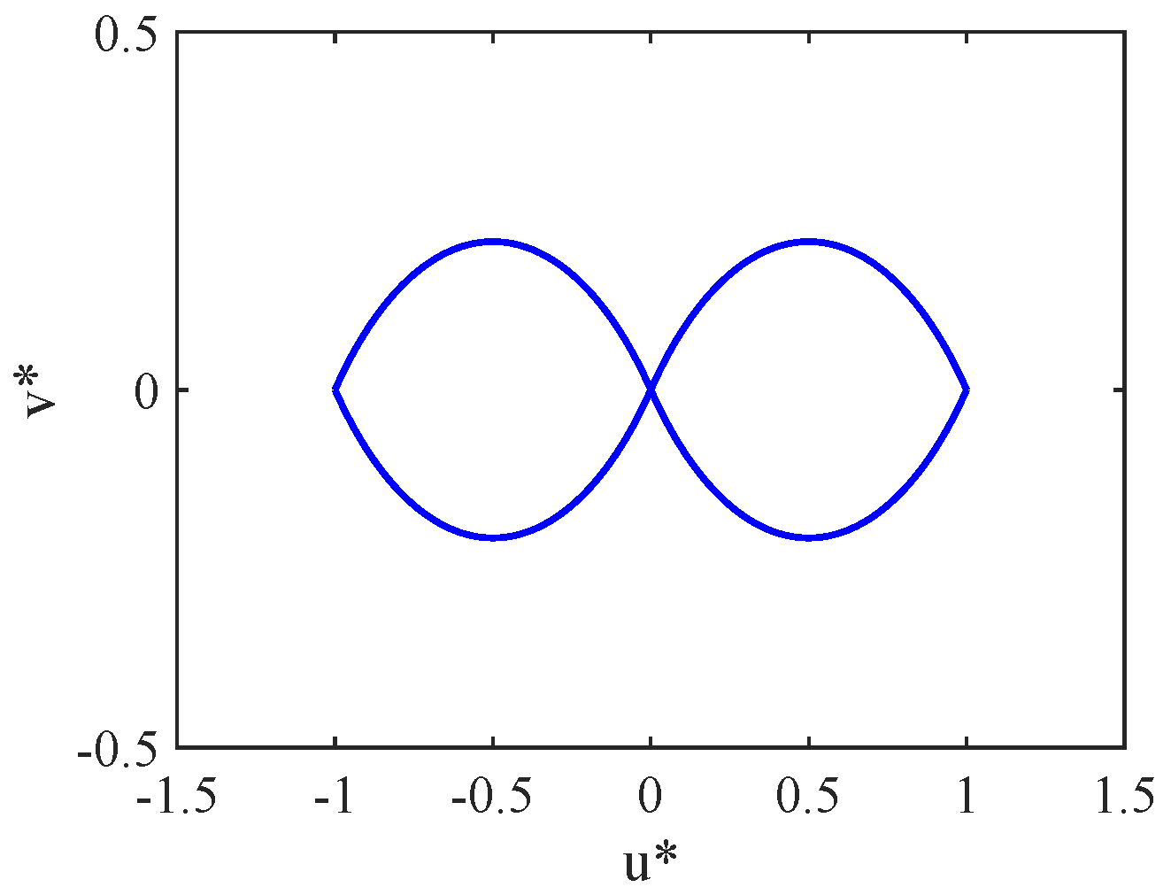
It is verified that system (7) has infinitely many equilibrium points $(u^{*},v^{*})$. These equilibrium points are located on the curve in the coordinate plane described by

$${\left(u^{*}\right)}^2-\left|u^{*}\right|+\left|v^{*}\right|+{\left(v^{*}\right)}^2=0.$$

(8)

It means that the new system (7) has eye-shaped curve equilibrium as shown in Figure 4. Note that the eye-shaped curve is different from some other shapes reported, such as line, square, circle, or cloud-shaped [11,19], and is symmetric about the u-axis, v-axis, and origin. Furthermore, system (7) has hidden attractors [17]. Above all, investigating system (7) will strengthen our understanding of hidden attractors.

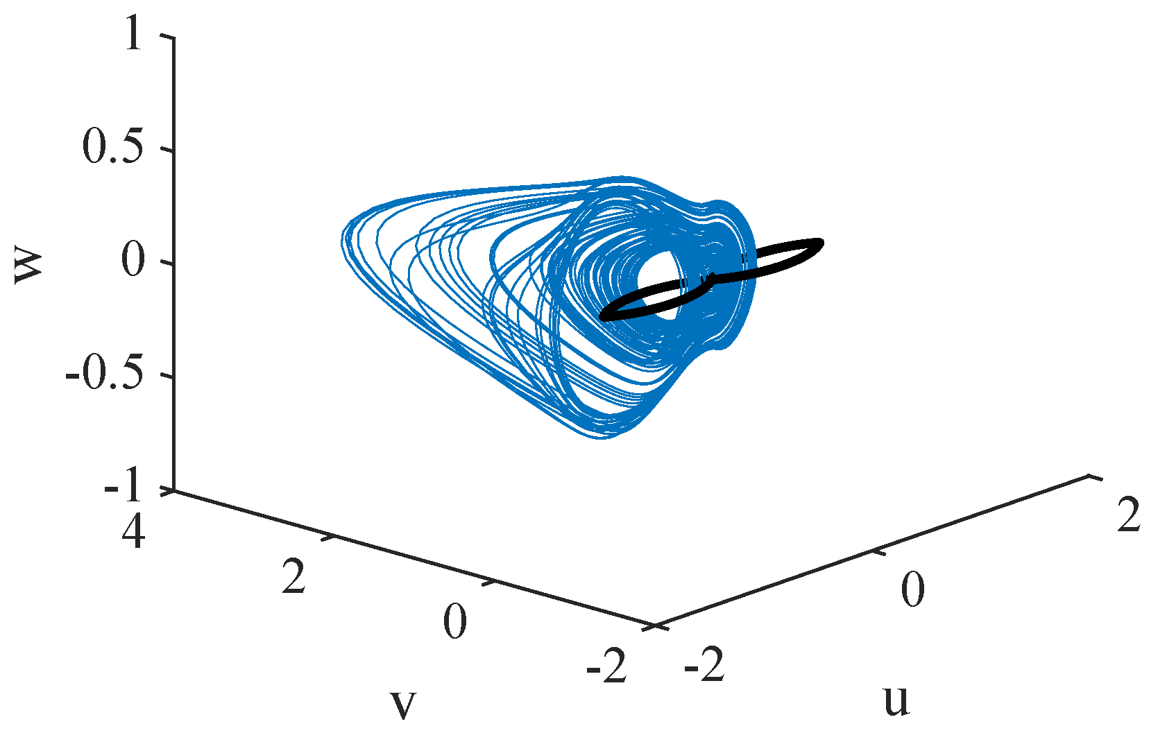
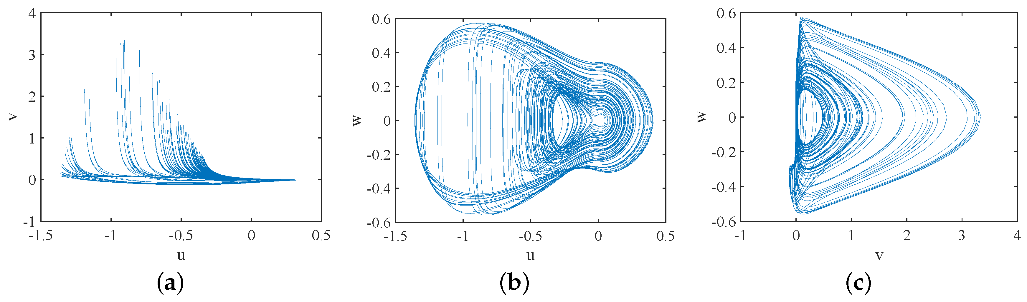
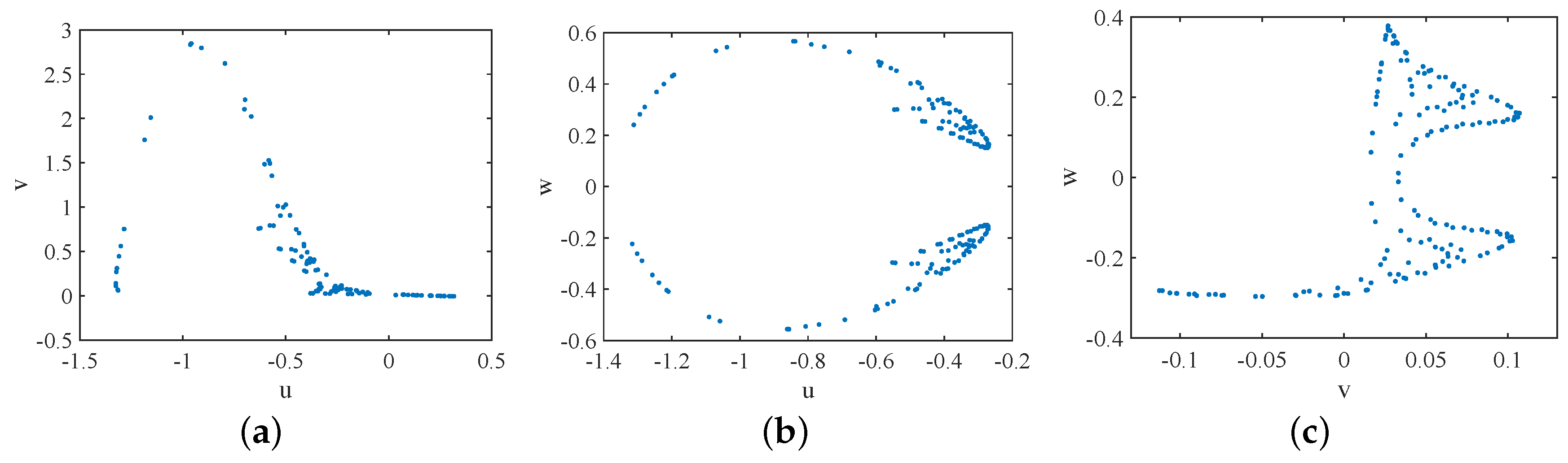
For $\alpha =5,\beta =30$, and initial conditions $(0.06,0.01,0.01)$, the new system (7) has chaotic attractors (see Figure 5 and Figure 6). For the simulation, we used the Wolf et al. method to calculate the Lyapunov exponents [20], the time of computation was 1000, and we obtained the Lyapunov exponents $(0.0424,0,-0.2484)$. The method of Wolf et al. is rooted conceptually in a previously developed technique that could only be applied to analytically defined model systems to monitor the long-term growth rate of small volume elements in an attractor. In addition, the corresponding Kaplan–Yorke dimension of system (7) is 2.1707. Poincaré return maps are often used to transform complicated behavior of a dynamic system in phase space to discrete maps in a lower dimensional space to reveal the complicated behaviors. Poincaré return maps corresponding with phase portraits in Figure 6 are presented in Figure 7; there are some dense points in the Poincaré section, and it can be determined that the motion is a chaotic state. These results reveal that the system is chaotic.

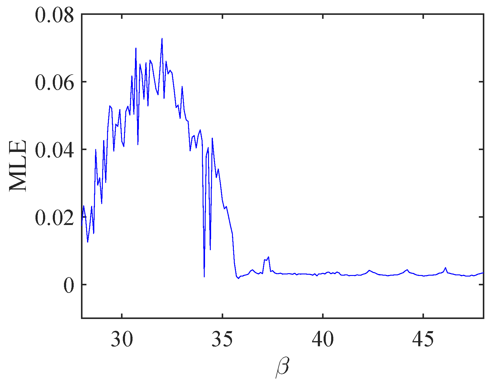
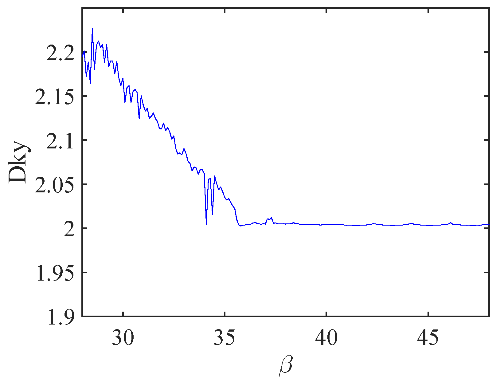
Gradually changing the value of the parameter $\beta$ or $\alpha$, the bifurcation plot of the system can be discovered in Figure 8. Figure 9 and Figure 10 reveal the diagram of Maximal Lyapunov Exponents and the diagram of Kaplan–Yorke dimension of system (7) for $\alpha =5,\beta \in [28,48]$, respectively.

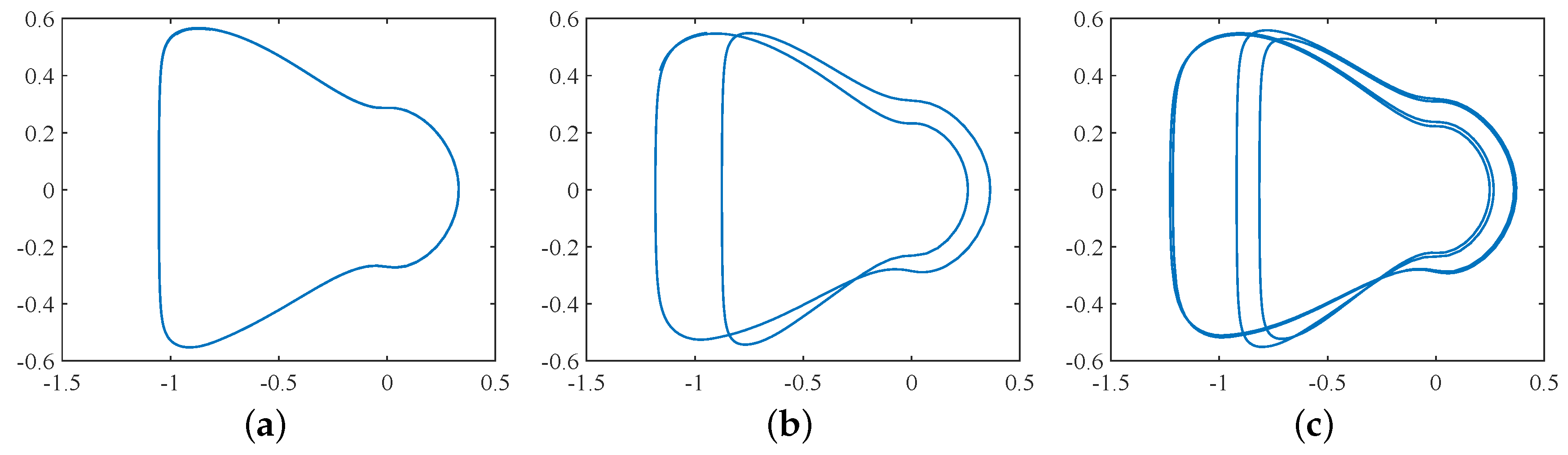
The new system with eye-shaped equilibrium has periodic behavior in the range $36\le \beta \le 48$. For instance, the system can display period-1 behavior for $\alpha =5,\beta =45$, period-2 behavior for $\alpha =5,\beta =38$, and period-4 behavior for $\alpha =5,\beta =36$ (see Figure 11a–c, respectively).

3. Anti-Synchronization of New Systems

Synchronization of chaos is a phenomenon that may occur when two, or more, dissipative chaotic systems are coupled. Since the pioneering work of Pecora and Carroll related to synchronization in chaotic systems [21], some methods of chaotic synchronization have been presented related to complete, generalized, lag, and imperfect phase synchronization [22]. Many papers on applications of chaos synchronization for cryptographic [23], kinetics [24], physiology [25], neural networks [26], and economics [27] have appeared.

In the following, we consider the anti-synchronization of the systems with eye-shaped equilibrium related to the driver-response system. The driver system with eye-shaped closed curve equilibrium is as follows:

$$\begin{array}{cc}\hfill \dot{u}& =w,\hfill \\ \hfill \dot{v}& =-w(\alpha v+\beta v^2+uw),\hfill \\ \hfill \dot{w}& =u^2-\left|u\right|+\left|v\right|+v^2,\hfill \end{array}$$

where u, v, and w are are three state variables, and the value of $\alpha =5,\beta =30$.

The response system is described as

$$\begin{array}{cc}\hfill {\dot{u}}_1& =w_1+h_1,\hfill \\ \hfill {\dot{v}}_1& =-w_1(\alpha v_1+\beta v_1^2+u_1{w}_1)+h_2,\hfill \\ \hfill {\dot{w}}_1& =u_1^2-\left|u_1\right|+\left|v_1\right|+v_1^2+h_3,\hfill \end{array}$$

(9)

where the control is $\mathbf{h}={[h_1,h_2,h_3]}^T$.

In order to reveal the difference between the driver system (7) and the response system (9), the state errors can be defined as

$$\begin{array}{cc}\hfill e_1& =u+u_1,\hfill \\ \hfill e_2& =v+v_1,\hfill \\ \hfill e_3& =w+w_1,\hfill \end{array}$$

(10)

and we obtain

$$\begin{array}{cc}\hfill {\dot{e}}_1& =\dot{u}+{\dot{u}}_1,\hfill \\ \hfill {\dot{e}}_2& =\dot{v}+{\dot{v}}_1,\hfill \\ \hfill {\dot{e}}_3& =\dot{w}+{\dot{w}}_1.\hfill \end{array}$$

(11)

Combining (7), (9), (10), and (11), we get the state errors system

$$\begin{array}{cc}\hfill {\dot{e}}_1& =e_3+h_1,\hfill \\ \hfill {\dot{e}}_2& =-w(\alpha v+\beta v^2+uw)-w_1(\alpha v_1+\beta v_1^2+u_1{w}_1)+h_2,\hfill \\ \hfill {\dot{e}}_3& =u^2-\left|u\right|+\left|v\right|+v^2+u_1^2-\left|u_1\right|+\left|v_1\right|+v_1^2+h_3.\hfill \end{array}$$

(12)

We choose the control proposed by

$$\begin{array}{cc}\hfill h_1& =-e_3-k_1{e}_1,\hfill \\ \hfill h_2& =w(\alpha v+\beta v^2+uw)+w_1(\alpha v_1+\beta v_1^2+u_1{w}_1)-k_2{e}_2,\hfill \\ \hfill h_3& =-u^2+\left|u\right|-\left|v\right|-v^2-u_1^2+\left|u_1\right|-\left|v_1\right|-v_1^2-k_3{e}_3,\hfill \end{array}$$

(13)

where $k_i>0(i=1,2,3)$ are the positive gain constants used to control the rate of anti-synchronization. By substituting (12) into (11), we get the state errors system

$$\begin{array}{cc}\hfill {\dot{e}}_1& =-k_1{e}_1,\hfill \\ \hfill {\dot{e}}_2& =-k_2{e}_2,\hfill \\ \hfill {\dot{e}}_3& =-k_3{e}_3.\hfill \end{array}$$

(14)

Obviously, the eigenvalues $(-k_1,-k_2,-k_3)$ of the Jacobian matrix of the state errors system are negative. Then, the complete anti-synchronization between the driver system (7) and the response system (9) is proved.

In numerical simulation, we assume the initial values of the driver system (7) and the response system (9) to be

$$\begin{array}{cc}\hfill u\left(0\right)& =0.06,\hfill \\ \hfill v\left(0\right)& =0.01,\hfill \\ \hfill w\left(0\right)& =0.01,\hfill \\ \hfill u_1\left(0\right)& =-0.20,\hfill \\ \hfill v_1\left(0\right)& =-0.09,\hfill \\ \hfill w_1\left(0\right)& =0.07.\hfill \end{array}$$

(15)

Then, the initial values of the state errors system (12) are

$$\begin{array}{cc}\hfill e_1\left(0\right)& =0.40,\hfill \\ \hfill e_2\left(0\right)& =-0.08,\hfill \\ \hfill e_3\left(0\right)& =0.08.\hfill \end{array}$$

(16)

The positive gain constants here are selected as $k_1=k_2=k_3=3$. It is obvious in Figure 12 that there exists anti-synchronization of the respective states of the new systems with two closed curve equilibrium (7) and (9). The time history of the synchronization errors $e_1,e_2,e_3$ is shown in Figure 13 which plots the anti-synchronization of the driver-response system.

4. Conclusions

In this work, we propose and study the following new system:

$$\begin{array}{cc}\hfill \dot{u}& =w,\hfill \\ \hfill \dot{v}& =-w(\alpha v+\beta v^2+uw),\hfill \\ \hfill \dot{w}& =u^2-\left|u\right|+\left|v\right|+v^2,\hfill \end{array}$$

(17)

with eyed-shaped equilibrium points which are located on two closed curves passing the same point. In Section 2, some dynamical properties of the proposed system are presented, which were investigated using bifurcation diagram, phase portrait, maximal Lyapunov exponents, and Kaplan-Yorke dimension. Furthermore, the anti-synchronization of systems is obtained by using active control in Section 3. This study will broaden the current knowledge of chaotic systems with infinitely many equilibria.

References

- Lorenz, E.N. Deterministic nonperiodic flow. J. Atmos. Sci. 1963, 20, 130–141. [Google Scholar] [CrossRef]
- Sprott, J.C. Some simple chaotic flows. Phys. Rev. E 1994, 50, R647–R650. [Google Scholar] [CrossRef]
- Sprott, J.C. Elegant Chaos Algebraically Simple Chaotic Flows; World Scientific: Singapore, 2010; pp. 10–11. [Google Scholar]
- Azar, A.T.; Vaidyanathan, S. Advances in Chaos Theory and Intelligent Control; Springer: Berlin, Germany, 2016; pp. 50–61. [Google Scholar]
- Pehlivan, I.; Moroz, I.M.; Vaidyanathan, S. Analysis, synchronization and circuit design of a novel butterfly attractor. J. Sound Vib. 2014, 333, 5077–5096. [Google Scholar] [CrossRef]
- Akgul, A.; Moroz, I.; Pehlivan, I.; Vaidyanathan, S. A new four-scroll chaotic attractor and its engineering applications. Optik 2016, 127, 5491–5499. [Google Scholar] [CrossRef]
- Pham, V.T.; Volos, C.; Jafari, S.; Wei, Z.; Wang, X. Constructing a novel no-equilibrium chaotic system. Int. J. Bifurc. Chaos 2014, 24, 1450073. [Google Scholar] [CrossRef]
- Molaie, M.; Jafari, S.; Sprott, J.C.; Golpayegani, S. Simple chaotic flows with one stable equilibrium. Int. J. Bifurc. Chaos 2013, 23, 1350188. [Google Scholar] [CrossRef]
- Jafari, S.; Sprott, J.C. Simple chaotic flows with a line equilibrium. Chaos Solitons Fractals 2013, 57, 79–84. [Google Scholar] [CrossRef]
- Gotthans, T.; Petrzela, J. New class of chaotic systems with circular equilibrium. Nonlin. Dyn. 2015, 81, 1143–1149. [Google Scholar] [CrossRef] [Green Version]
- Gotthans, T.; Sprott, J.C.; Petrzela, J. Simple chaotic flow with circle and square equilibrium. Int. J. Bifurc. Chaos 2016, 26, 1650137. [Google Scholar] [CrossRef]
- Pham, V.T.; Jafari, S.; Volos, C.; Giakoumis, A.; Vaidyanathan, S.; Kapitaniak, T. A chaotic system with equilibria located on the rounded square loop and its circuit implementation. IEEE Trans. Circuits Syst. II Express Briefs 2016, 63, 878–882. [Google Scholar] [CrossRef]
- Zhu, X.; Du, W.-S. A new family of chaotic systems with different closed curve equilibrium. Mathematics 2019, 7, 94. [Google Scholar] [CrossRef]
- Bondarenko, V.E. Information processing, memories, and synchronization in chaotic neural network with the time delay. Complexity 2005, 11, 39–52. [Google Scholar] [CrossRef]
- Cicek, S.; Ferikoglu, A.; Pehlivan, I. A new 3D chaotic system: Dynamical analysis, electronic circuit design, active control synchronization and chaotic masking communication application. Optik 2016, 127, 4024–4030. [Google Scholar] [CrossRef]
- Leonov, G.; Kuznetsov, N.; Seldedzhi, S.; Vagaitsev, V. Hidden oscillations in dynamical systems. Trans. Syst. Contr. 2011, 6, 54–67. [Google Scholar]
- Dudkowski, D.; Jafari, S.; Kapitaniak, T.; Kuznetsov, N.V.; Leonov, G.A.; Prasad, A. Hidden attractors in dynamical systems. Phys. Rep. 2016, 637, 1–50. [Google Scholar] [CrossRef]
- Sprott, J.C. A proposed standard for the publication of new chaotic systems. Int. J. Bifurc. Chaos 2011, 21, 2391–2394. [Google Scholar] [CrossRef]
- Wang, X.; Pham, V.T.; Volos, C. Dynamics, circuit design, and synchronization of a new chaotic system with closed curve equilibrium. Complexity 2017, 2017, 7138971. [Google Scholar] [CrossRef]
- Wolf, A.; Swift, J.B.; Swinney, H.L.; Vastano, J.A. Determining Lyapunov exponents from a time series. Phys. D Nonlinear Phenom. 1985, 16, 285–317. [Google Scholar] [CrossRef] [Green Version]
- Pecora, L.M.; Carroll, T.L. Synchronization in chaotic systems. Phys. Rev. Lett. 1990, 64, 821–824. [Google Scholar] [CrossRef]
- Boccaletti, S.; Kurths, J.; Osipov, G.; Valladares, D.L.; Zhou, C.S. The synchronization of chaotic systems. Phys. Rep. A 2002, 366, 1–101. [Google Scholar] [CrossRef]
- Klein, E.; Mislovaty, R.; Kanter, I.; Kinzel, W. Public-channel cryptography using chaos synchronization. Phys. Rev. E 2005, 72, 016214. [Google Scholar] [CrossRef] [PubMed]
- Li, Y.N.; Chen, L.; Cai, Z.S.; Zhao, X.Z. Experimental study of chaos synchronization in the Belousov-Zhabotinsky chemical system. Chaos Solitons Fractals 2004, 22, 767–771. [Google Scholar] [CrossRef]
- Glass, L. Synchronization and rhythmic processes in physiology. Nature 2001, 410, 277–284. [Google Scholar] [CrossRef] [PubMed]
- Zhang, X.H.; Zhou, S.B. Chaos synchronization for bi-directional coupled two-neuron systems with discrete delays. Lect. Notes Comput. Sci. 2005, 3496, 351–356. [Google Scholar]
- Yousefi, S.; Maistrenko, Y.; Popovych, S. Complex dynamics in a simple model of interdependent open economies. Discret. Dyn. Nat. Soc. 2000, 5, 161–177. [Google Scholar] [CrossRef] [Green Version]
Figure 1.
The circle-shape of equilibrium points of system (3) in the plane .
Figure 2.
The cloud-shape of equilibrium points of system (4) in the plane .
Figure 3.
Different shapes of equilibrium points of system (5), k = 1, 2, 3, 4, 5, from the interior to the outside, respectively, in the plane .
Figure 4.
The eye-shape of equilibrium points of system (7) in the plane .
Figure 5.
3D view of the chaotic attractor and eye-shape of equilibrium points located in the plane w = 0 of system (7) for .
Figure 6.
The projection of the trajectory of system (7) in (a) u-v plane, (b) u-w plane, (c) v-w plane for .
Figure 7.
The Poincaré section of system (7) for (a) , (b) , (c) for .
Figure 8.
Bifurcation plot of system (7) for (a) and (b) .
Figure 9.
Maximal Lyapunov Exponents spectrum of system (7) for .
Figure 10.
Kaplan–Yorke dimension of system (7) for .
Figure 11.
Periodic behavior of system (7) in the u-w plane: (a) period-1 , (b) period-2 , (c) period-4 .
Figure 12.
Anti-synchronization of the driver-response system: (a) , (b) , (c) , the driver system (dashed lines), the response system (solid lines).
Figure 13.
Time history of the anti-synchronization of the state errors system: (a) , (b) , (c) .
© 2019 by the authors. Licensee MDPI, Basel, Switzerland. This article is an open access article distributed under the terms and conditions of the Creative Commons Attribution (CC BY) license (http://creativecommons.org/licenses/by/4.0/).
Share and Cite
MDPI and ACS Style
Zhu, X.; Du, W.-S. New Chaotic Systems with Two Closed Curve Equilibrium Passing the Same Point: Chaotic Behavior, Bifurcations, and Synchronization. Symmetry 2019, 11, 951. https://doi.org/10.3390/sym11080951
AMA Style
Zhu X, Du W-S. New Chaotic Systems with Two Closed Curve Equilibrium Passing the Same Point: Chaotic Behavior, Bifurcations, and Synchronization. Symmetry. 2019; 11(8):951. https://doi.org/10.3390/sym11080951
Chicago/Turabian StyleZhu, Xinhe, and Wei-Shih Du. 2019. "New Chaotic Systems with Two Closed Curve Equilibrium Passing the Same Point: Chaotic Behavior, Bifurcations, and Synchronization" Symmetry 11, no. 8: 951. https://doi.org/10.3390/sym11080951
Note that from the first issue of 2016, this journal uses article numbers instead of page numbers. See further details here.