Extracting Information from an Urban Network by Combining a Visibility Index and a City Data Set


1
Department of Computer Science and Artificial Intelligence, University of Alicante, Campus de San Vicente, Ap. Correos 99, E-03080 Alicante, Spain
2
Department of Expresión Gráfica, Composición y Proyectos, Campus de San Vicente, Ap. Correos 99, E-03080 Alicante, Spain
*
Author to whom correspondence should be addressed.
Symmetry 2019, 11(5), 704; https://doi.org/10.3390/sym11050704
Submission received: 28 March 2019
/
Revised: 15 May 2019
/
Accepted: 20 May 2019
/
Published: 23 May 2019
Abstract
:Cities can be represented by spatial networks, and the mathematical structure that defines a spatial network is a graph. Taking into account this premise, this paper is focused on analysing information on an urban scale by combining a new ray-casting visibility index with a data set of the urban street network. The visibility index provides information about the most visible buildings or areas. We relate this index with other data extracted from the city, with the aim of generating and analysing information about urban elements. To corroborate this idea, real data are analysed. The dataset is related to the heritage conservation of the buildings of the Villaflora suburb, located in the city of Quito (Ecuador). This information is processed, together with the visibility index, with the aim of determining the conservation degree of the urban areas most visually exposed to pedestrians or visitors. The combination of both values—heritage conservation and visibility index—is carried out by means of two new indices, and , which are defined using two-variable exponential functions.
1. Introduction
1.1. Motivation
Cities are complex systems, involving multiple aspects which need to be studied from a multi-disciplinary approach. For that purpose, several authors have proposed the use of intellectual tools, coming from the so-called sciences of complexity [1]. Therefore, it is possible to find several research works which have applied different aspects of chaos theory, models based on emerging systems [2], or fractal geometry [3,4,5], for instance, to understand urban landscapes [6]. In this regard, one of these approaches comes from the application of network theory to this sort of urban study. Extracting and describing information from a network is one of the main goals of science, and the study of networks currently draws the attention of several fields of research. From this point of view, urban studies propose to understand cities as a complex network, constituting systems where large amounts of information and data are generated constantly. The sources of this vast information can be very diverse; for example, data could be collected from field-work, from Web services supported by social networks, or from existing databases (open or protected). To deal with all this data, we find that many different kinds of models and algorithms can be applied.
In this study, we chose visibility as a crucial aspect of the urban context, because the issue we want to study is urban heritage, and it is not possible to decide, for a society, which existing elements should be preserved or not, if they are not visible. This is just of the reasons why it may be quite relevant for urban designers and researchers to analyse the visibility of urban spaces [7,8]. Visibility analysis has been proved to be useful in investigating urban environments in general, allowing researchers to form mathematical descriptions of systems which complements other phenomenological approaches, hence enabling us to predict the inhabitant experiences in urban environments with reasonable certainty [9,10]. In visibility analysis, it is important to have metrics that characterize different aspects of the visibility relationships. For instance, through the development of visibility metrics, it is possible to establish the visible extent of landmarks in an urban environment [11].
1.2. Literature Review
In order to study a network, we first need to represent it with an abstract model, and then extract from the model some information not provided a priori [12]. We represent a network as a spatial mathematical graph, composed by a set of nodes linked by a set of edges. The most common approach to the spatial representation of an urban network is by using the concept of a primal graph [13], in which the edges are defined by streets and the nodes are intersections.
Historically, the environment is describable as fused with space, given the strong interrelation between space, light, and visibility. This interrelation leads us to the concept of isovists [14], which has been presented as a methodology for recording landscapes [15].
From a conceptual point of view, an isovist is a way of representing the amount of space that is visible from a particular vantage point. Therefore, an isovist is the set of all points visible from a given vantage point in some environment. Isovists represent the entirety of the visible plain (in 2D) or volume (in 3D) at a specific point in space, bounded by the built environment. Every point in physical space has an isovist associated with it [16]. In [17], Benedict introduced a set of analytical measurements of isovist properties that can be applied to achieve quantitative descriptions of spatial environments. Subsequently, perception of space was shown to be affected by some isovist attributes [18].
An isovist is a geometric, and thereby measurable, representation of the experience of human sight. The visible space that the isovist records is typically close to a horizontal slice, taken parallel to the ground at eye-height, through the 3D visible volume [17]. Once the 2D isovist has been developed, then it is possible to quantitatively analyse its geometry to obtain various insights into the design properties of an architectural plan ([14,19]). While 2D isovist analysis has dominated this field of inquiry, other researchers have set out to include the third dimension [20,21]. Such research seeks to capture the visual properties of an entire space from a defined location.
It’s known that view-shed analysis is an important tool used to describe the visible spatial structure of an environment. In the field of Geographic Information System (GIS), view-shed analysis has proved to be the most popular methodology for quantifying visibility ([19]), and its application is common-practice in a range of fields, including archaeology [22], urban planning [23], and so on. We must recall that, Tandy (1967) introduced the view-shed and, it was implemented in a computer program to automatically quantify visibility across terrain in 1968 [24]. In this analysis, the visibility is quantified by generating the Lines of Sight (LoS) between an observer point and all cells of a grid.
Isovists and view-sheds differ in their methodologies and their applications [25]. The isovist term is used generally in built environments with vector data while a visibility graph can be calculated with different characteristics (view quality or perimeter compactness). On the other hand, the view-shed term is more commonly used to calculate the intervisibility in a rural environment, with raster data.
In 1984, a new development in visibility relationships was introduced into graph analysis of buildings [26]. The general idea is that spaces can be broken down into different components, analysed as networks of choices, and then represented as maps and graphs describing the relative connectivity and integration of those spaces. The approach was based on the concept of axial lines in urban networks, which are the fewest and longest lines of sight and represent rings of circulation in the street network. This is the Space Syntax model [27,28], which encompasses a set of theories and techniques for the analysis of spatial configurations and the visualization of urban networks. It defines the model of an axial map to quantify and compare accessibility patterns of an urban space [29]. In Space Syntax, there appears the important concept of a visibility graph [19,30], which can be defined as a graph where each node represents a point location, and each edge represents a visible (without obstacle) connection between two nodes.
1.3. Main Contribution
The objective of this paper is to analyse information in an urban scale using a new visibility index. With this objective, we combine a new ray-casting based visibility index with data acquired in an urban environment.
The visibility index developed in this work is based on the fact that two points are mutually visible if the line of sight joining them does not intersect the interior of any obstacle. To elaborate the visibility index, we use a graph of visibility composed by the nodes of a primal graph of a city and points of a grid located in the facade of the buildings.
The new visibility index determines those buildings that are more visible, and is used to obtain additional information when it is associated with other urban data. To this purpose, we use a data set obtained in a Quito suburb, called Villaflora, combined with the visibility numerical values of the mentioned neighbourhood. This link is carried out by means of two new indices, and , which are defined using two-variable exponential functions. Both indices allow for the determination of specific buildings that must be preserved ( index); and buildings that could be renovated ( index) to improve the image of the neighbourhood. Therefore, we extract information from the urban network, establishing a relationship between a visibility index and the heritage conservation value of each building.
For this purpose, the paper is organized into five sections. Following this introduction, there is a detailed description of the methodology used in the paper. Starting with the proposed visibility index and the city dataset about heritage conservation, a combination of both is made through the two new metrics. The third section presents the numerical results of the new two indices in a real case study. The fourth section is related to the discussion of the advantages and disadvantages of the proposed measures. Finally, some conclusions are presented.
2. Methodology
Figure 1 shows a scheme of the key points of the model, in which we highlight three main elements that indicate the essential points.
2.1. The Visibility Index V
This sub-section presents an index, in order to establish the visibility metric with the ability to map which areas are more visible. With this goal, a numerical value for each building, called the visibility index, V, is described. This index quantifies the degree of visibility, within the urban network, each building has. To achieve this objective, a ray-casting technique [31] is used. This method has been applied in a wide variety of problems; for example, in medicine visualization [32], tracing frameworks for scientific visualization [33], or modelling distant pointing for compensation [34], among others.
Given a set of obstacles in Euclidean space, two points in the space are visible to each other if the line segment that joins them does not intersect any obstacles. With this in mind, this technique consists of spreading a bunch of rays from a specific source to specific targets and, then, identifying all targets that received unobstructed rays.
It should be noted that, in this technique, the distance between the ray source and the targets is not important, since the objective is to see the number of rays that are not obstructed.
Before the description of the index, it is necessary to develop a mathematical model capable of summarizing all data related to the city. The main purpose of such a model is to simplify the complexity of an urban system by selecting the most relevant characteristics for the study in question. The most suitable model for urban space discretization is a graph. In order to represent the urban space through a graph, different approaches [13,35] can be taken. In this study, the mathematical structure used is a primal graph, since this graph is the one that best reflects the geometrical characteristics of the urban network [35,36]. The primal graph is constructed with vertices (intersections of streets) and edges (streets). Figure 2 shows a primal graph (made in the Rhinoceros software) associated to an urban network.
With the index presented in this section, we want to establish a visibility value for each building of the urban plot, taking into account the geometry that defines the urban layout. To begin with, we consider the example in Figure 3, with three buildings of different sizes and the path that follows the nodes of the primal graph. If the path given by the points is followed, the blue building is the least visible, since it is covered by the others, and the orange one is the most visible, since it is the most exposed to the path of points .
The visibility of each building can be assessed by means of an index; however, the fact that not all of the building faces are equally visible must be taken into account, and constitutes a determining factor in the proposed model.
The starting point in the model is a set of vertices
which are the nodes of the primal graph associated with the studied urban network. The example of Figure 3 has 5 nodes
The basic idea of this model is to take every building and assign to it a uniform grid, as shown in Figure 4a. This grid is divided into points, which are separated from each other by a constant number that is at unit distance. Consequently, each building has a grid associated to it, denoted by .
In order to see all the points of the grid that are used in the calculation of the index, a flat representation of each building can be obtained by unfolding the grid, as shown in Figure 4b. Thus, every point of the grid associated to the building is denoted as , where i represents the building identifier and j represents the point grid identifier. Therefore, we can establish a correspondence
The following step consists of assigning a numerical value to every point of the grid . This integer value, denoted as , provides the number of unobstructed rays from every point of P. In our case, the ray source is the set of nodes of the primal graph and the targets are the grid points (see Figure 4a). Therefore, a correspondence can be established,
where every point in the grid has an associated integer, , representing the number of unobstructed rays from all the nodes of the primal graph. Consequently, is the number of points of the primal graph visible from each node of the building. Adopting this approach, a parameter associated to each building, which represents a local discrete distribution of the visibility in each point of the grid, is calculated. The next step is to establish a unique value of visibility for the entire building. For this purpose, the average of all values is computed
In this index, the element represents, for the building i and point j of the grid, the number of unobstructed rays from all nodes of the primal graph. Taking the summation for every element of the grid, we obtain a value for each building. Finally, it is necessary to normalise the measure, by dividing by the total number of points in the grid.
In the example of Figure 4a, the small building () is discretized by a grid consisting of 5 faces on 9 points each; so, the grid is
Note that, in this example, only two points of the primal graph are considered (the points A and B). Therefore,
Summarizing, for each building i of the urban layout object to study, a visibility index has been proposed.
A practical application of this index was made, using proprietary software made in C/C++.
2.2. Data Acquisition for the Heritage Area
The heritage relevance of the area of study has been explained in [37], where the methodology of data acquisition through fieldwork was also described. In this last aspect, in the present work, this kind of approach (which is usually accepted in heritage fieldwork) was followed. From the UNESCO criteria for heritage elements [38], to the European Union with its European Heritage Label [39], and to any local regulation in this matter, architectural heritage protection has been historically expressed in catalogs. Those documents describe the urban and architectural elements that should be protected and the level of protection, and translating quality conditions into quantitative figures [40]. As a consequence, this is a process which necessarily implies the evaluation of each element to be protected by a heritage specialist, who analyses its particular conditions and determines, from a certain point of view, its relevance. This process is, therefore, subjective in many aspects, and needs extensive fieldwork which cannot be avoided, given the sensitive nature of the analysed matter.
The criteria related to the heritage condition of the elements followed by this paper depends on what has been established in the literature about architectural heritage. In this sense, the publication [41] has been usually accepted, in the discipline of architectural heritage, as a reference. It has been widely proposed, in the heritage literature, the importance of some ornamental elements (such as window frames or decorative cornices, for instance) in characterising some specific architectural language. For this reason, even those elements that have a minor importance, from a distance, are quite relevant to the definition of the heritage condition of the building.
The contribution of this part comes from the proposal of defining an objective theoretical framework to evaluate the architectural elements. This framework is based on a system of indicators formed by all the relevant parameters that contribute to identifying an urban model (see Table 1). This is a technique normally used in urban analysis [42]. By adapting this methodology to the evaluation of heritage condition, it is possible to establish a clear protocol of action to be applied to the changing conditions in the area through the years, regardless of who is developing the survey for the heritage protection of the suburb.
Given these indicators, extensive fieldwork, in order to identify each architectural element in every building, was performed in the suburb of Villaflora (Quito) (see Figure 5). The urban area of Villaflora has 795 plots and, to better organize the fieldwork, the urban layout was divided into sectors. A fact-sheet was produced for each plot, in which a photo, the sector location, and the values of the heritage indicators were included, as shown in Figure 6.
As a consequence of the field study carried out on the heritage conservation values of the Villaflora buildings, a numerical value () value) was obtained for each building.
2.3. Processing Information from the Visibility Index
The objective of the paper is to obtain information about the city by establishing a relationship between the visibility index (V) and the data of the urban layout. Our dataset is the heritage conservation level () of each building of the Villaflora suburb. However, establishing a relationship between the heritage conservation value of a building and its visibility requires a mathematical approach, which is performed by means of two new indices.
The link between the visibility index and heritage value should enable an evaluation of the degree of conservation of the urban areas most visually exposed to pedestrians. To establish this association, it must be taken into account that both of the values and V are normalized to between 0 and 1, which makes it easier to look for relations between them.
The final goal of this section is to offer a rational and objective approach, which may help public institutions to know where and how to act in the area. In our case study, a map with the most visible buildings with high heritage values and a map with the most visible buildings with low heritage values were produced. With this model, it is possible to identify where some transformations may have more impact for the network than others. If we take into consideration that public resources are always limited, this information may be quite helpful to identify where the public institutions should be especially careful in protecting some buildings (because their transformations will affect negatively the area) or, on the other hand, where some restorations will be particularly strategic, when compared to others; understanding that they will have a global impact.
2.3.1. The Index
The idea of the index consists of mixing the concepts of heritage conservation and visibility, focusing on those buildings with both high indices of and V.
The first idea that comes to mind is to take a linear function for the index
where is the heritage conservation value and the visibility index. In this case, as it is a linear function, the increases (decreases) are proportional.
However, our objective is to reward the increase of the index when the value of both variables are greater. For this purpose, the exponential function adapts perfectly. Furthermore, if we want to give more or less importance to both parts of the index, we need to consider the inclusion of a parameter. With this in mind, the index of a building , with heritage conservation value and visibility index , is defined as
where is a parameter in the range .
Analysing Equation (2), we realize that the index is always less than or equal to and, therefore, the optimal index value occurs when and .
It can be observed that . For instance, when , the index is located in the interval ; meanwhile, when , the index is located in .
The idea behind the definition of the parameter is to control the contraction experienced by the index against the original value , especially when the value of the visibility is low.
On one hand, when the visibility value is high, the variations between the index and the heritage conservation value are not large and, thus, if , then . On the other hand, when the visibility is low, we can penalize the index by means of the parameter. For instance, if the visibility is zero, .
Figure 8 shows these characteristics. On the left, the functions , for different values of are presented; while, on the right, the same functions for are presented.
When the value of is low (as in the left side of Figure 8), the index takes low values when the visibility index is also low, regardless of the value of .
Therefore, for low values of the parameter , the index is penalized when the visibility is low, without influencing the original heritage conservation value for the final result of the index.
Another feature, as can be observed from the graphs, is that there are not many items with high values approaching the maximum ().
Taking into account the right side of the Figure 8, for a high value of , the appearance of the graphs with different values of (i.e., horizontal lines), indicates that if the range of values of the index is small, we have extreme values for visibility.
For intermediate values of visibility (around ), we realize that we can find index values above , provided that is or greater.
2.3.2. The Index
The idea behind the definition of the index was motivated by the interest in those buildings with the high index of heritage value and high index of visibility. In this sub-section, the opposite approach is used to define the index; which is intended to find those buildings that have a very low heritage conservation and a high visibility index V.
These elements cause a negative influence on the urban environment and, taking into consideration that public resources are always limited, it is quite helpful to identify where the public institutions should do some strategic restorations; understanding that they will have a global impact.
Assuming that each building has the values and , then the index is defined by
As in the previous sub-section, if and , it is clear that .
A fundamental and basic difference between and must be noted: The maximum value of the index is ; whereas that of the index is . Basically, elements with a higher value of are those with a lower and higher .
The value of the index is the result of adding a quantity related to the heritage conservation value () and another quantity related to the visibility index (). The quantity related to the heritage conservation is , while the quantity related to visibility is given by the exponential curve.
In Table 2 some numerical results are presented. The columns of Table 2 represent: The index, the index, the parameter , de heritage conservation , and the visibility index . We have taken extreme values for these parameters, in order to better understand the behaviour of these indices.
Several facts must be highlighted: The highest values of are reached for the highest values of and , and the highest values of are reached for the lowest value of and the highest value of . The influence of the visibility value is more remarkable when the parameter is lower.
3. Results
In this section, a case study of Villaflora is presented, using a combination between the heritage values and the visibility index by means of the two new indices and .
The value represents the heritage conservation state of each building, normalized between 0 and 1 to facilitate the analysis. The blue areas of Figure 9 show buildings with low heritage conservation index values and, conversely, the yellow plots were better preserved. Note that there were 355 buildings with a null heritage conservation value, which represents a very considerable amount.
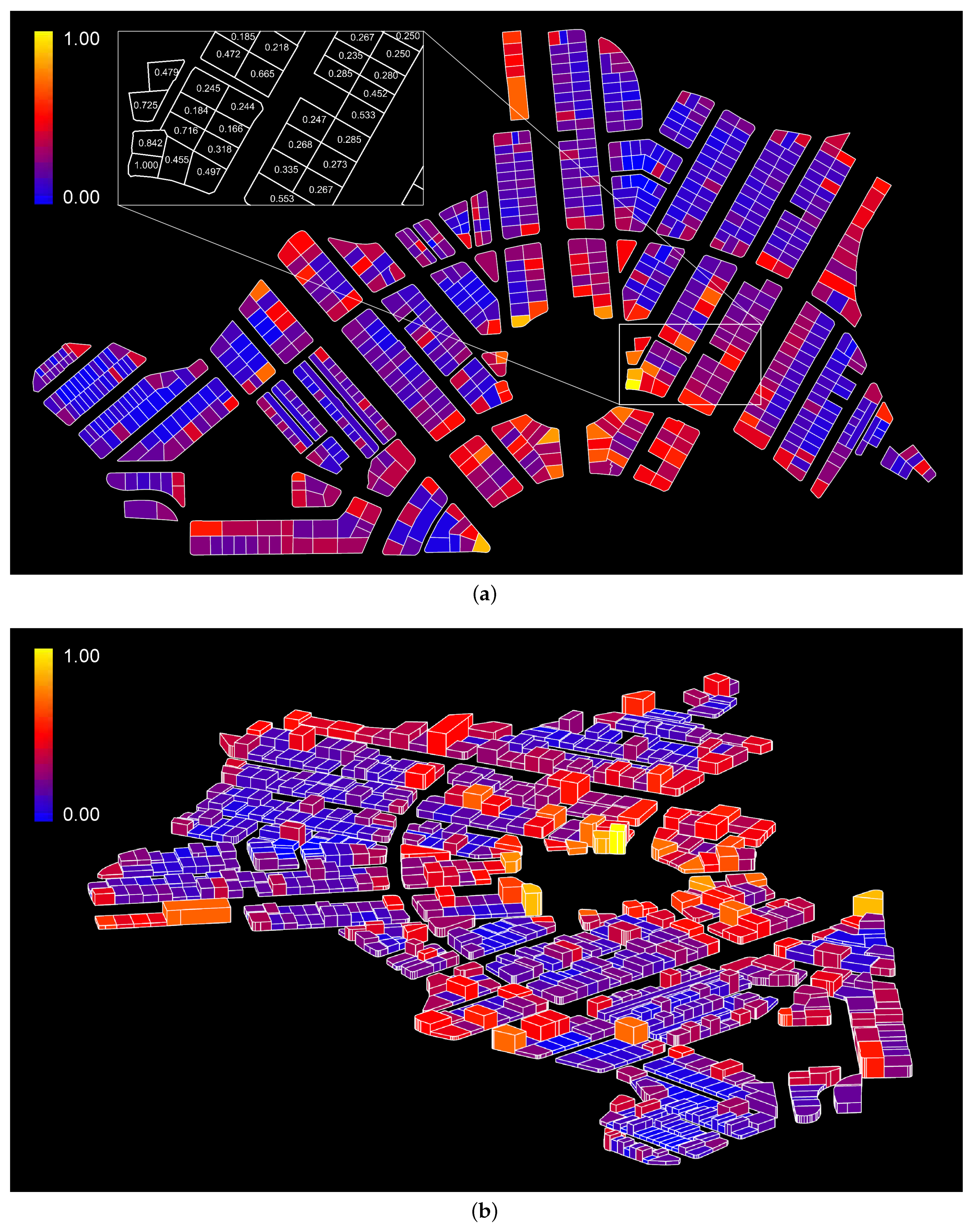
On the other hand, the visibility index depends on the topological structure of the studied urban network, since the points we use to draw the rays are nodes of the primal graph (intersections of streets). Applying the expression (1) to each building, a value for the visibility index of each building is obtained. The numerical results for the 795 buildings are shown graphically in Figure 10, where a chromatic scale is used. Blue areas predominate, which means that, from the nodes of the primary graph, there are many buildings with very low visibilities. On the contrary, as a result of the particular topology of the studied urban network, where there is a large roundabout and several main streets that depart from it, we observe buildings with a higher visibility index (yellow–orange area) in that area.
The values are normalized between 0 and 1, so as to limit the dispersion range.
A quantitative analysis of the visibility index, with a histogram of frequencies (see Figure 11) and some basic statistical parameters was performed in Table 3.
The histogram of Figure 11 shows a normal distribution of the data around its average value and the statistical parameters show that the data not widely spread, with regards to the mean. This is clearly shown by the kurtosis value. This number implies a concentration of values close to the mean and far from the tail.
With the data that feeds the new indices, the two indices are calculated (using Equations (2) and (3)). The index focuses on providing the elements with a greater importance, in terms of heritage conservation and high visibility, and the index determines buildings with low heritage conservation value but which are located in important places, in terms of their visibility.
As a result (see Figure 12), both indices were applied to the 795 urban plots of the suburb. In Figure 12a, the index values for all buildings of the suburb are shown. According to the established chromatic scale, yellow and orange buildings represent the highest indices, which means that they are buildings that preserve their heritage value and are located in visible areas within the urban network.
It is worth noting that, for the calculation of the indices in Figure 12, the value of the parameter in Equations (2) and (3) was . This means a neutral value, in terms of the importance it gives to the level of visibility of each of the buildings.
Comparing the local visibility map in Figure 10a and the index of Figure 12a, we observe the differences between a local measure (the visibility index) and an index that links concepts. For instance, the yellow buildings show those that the authorities must preserve, exhibit, and promote to the public wanting to visit the neighbourhood with the aim of appreciating the original buildings of the suburb.
Figure 12b shows the index values, using the same chromatic scale. The buildings with the highest values of are visualized in yellow and represent buildings with low heritage values located in high visibility areas. Similarly, we can compare the local heritage conservation map shown in Figure 9 and the index of Figure 12b. This comparison also shows the differences between a local urban measure (the heritage conservation value) and an index that links concepts. In this case, the yellow buildings are those that the authorities should restore to improve their appearance.
As a example, in Figure 13, the fact sheets of the two plots with the highest index and are shown.
4. Discussion
The urban planning and architecture of the Villaflora suburb constitutes an important heritage resource. In this sense, buildings with a high value of the index—very visible buildings with a different aspect with respect to the original one—suppose a negative impact on the image of the neighbourhood. Therefore, the heritage value of the suburb is highly affected by them.
On the other hand, buildings with a high value of the index constitute the reference buildings for the local architecture of the neighbourhood, given that they preserve their original aspect and are very exposed to pedestrians.
We must say that this kind of analysis does not substitute for other sorts of approaches. In this sense, it is necessary to mention that other conditions, such as those related to human perception or the environment, should also be taken into account, in order to decide how to act in some heritage areas. These should be considered, as well as social and economical conditions, among others.
However, even considering these limitations, it seems clear that the present research provides specialists with very relevant information about the impact of some possible actions to be implemented in the neighbourhood. From this point of view, this visibility index may constitute, for public institutions (which are usually responsible for urban actions in heritage areas), strategic information to be included with the rest of their considerations.
This work is a part of a more complex urban research, sponsored by the Government of Ecuador under its Prometeo Program. The aim of this research is to provide a tool that helps architects and governmental bodies to make decisions in some singular parts of the city; in this case, the city of Quito. Those parts of the city which have urban heritage, despite their lack of monumental buildings. Due to this lack, heritage considerations are not obvious on a first approach, and it is necessary to generate multiple data expressing the qualitative aspects of the area.
The final goal of this case study is to offer a rational and objective approach, which may help public institutions to know where and how to act in the area. Offering a map with the most visible nodes, it is possible to identify where some transformations may have more impact for the network than others. If we take into consideration that public resources are always limited, this information may be quite helpful to identify where the public institutions should be especially careful in preserving some buildings (because their transformations will affect negatively the area) or, on the other hand, where some restorations will be more strategic than others; understanding that they will have a global impact for the urban network.
5. Conclusions
Our starting point is to analyse information from urban environments by using a new visibility index. This index provides us with information about which buildings are more visible, and may be used to generate more information about other urban aspects when it is related with data extracted from the city.
A case study is shown for a Quito neighbourhood called Villaflora. This study is developed using normalized data collected about the heritage conservation of all the buildings of the suburb. The combination of heritage conservation and visibility numerical values is carried out by means of two new indices, and , which are defined using two-variable exponential functions. According to the definition of these indices, we are able to give more or less influence to the two measures studied (visibility and heritage conservation).
When these measures are applied to the individual elements or buildings, we get a classification of them, in the range . The buildings with the highest index are those with the highest heritage conservation index and high visibility, while the buildings with the highest index are those with the lowest heritage conservation index and high visibility.
According to the study, a few conclusions have been drawn from the current research of the authors. The visualization of the indices provides valuable and diverse information. On one hand, the visualization shows some areas that are undergoing important degradation, with respect to heritage conservation. On the other hand, both indices allow for identification of negative buildings, which damage the neighbourhood image (degraded buildings with high visibility) and, also, the buildings that are well preserved and very visible in the Villaflora suburb.
The innovation of this method appears in the connection between local data from a city (heritage conservation) and visibility in the same city. This allows us to determine the degree of conservation of the urban areas most visually exposed, with the ultimate goal of targeting potential building renewal sites. Obviously, the final decision of where or what kind of action (preservation, renovation, demolition, and so on) should be taken, depending on the combination of factors from different viewpoints. There are aesthetic, social, economical, and phenomenological reasons, among others, which may be taken into consideration for this purpose. For this kind of complex decision, this research provides a layer of relevant information, from the point of view of heritage quality in urban spaces.
Author Contributions
All authors contributed equally to this work: conceptualization, methodology, formal analysis, investigation, and writing–original draft preparation.
Funding
This research is partially supported by the Spanish Government, Ministerio de Economía y Competividad, grant number TIN2017-84821-P.
Conflicts of Interest
The authors declare no conflict of interest.
References
- Jenkens, C. The Architecture of the Jumping Universe. How Complexity Science is changing Architecture and Culture; Wiley: London, UK, 1997. [Google Scholar]
- Jonshon, S.J. Emergence: The Connected Lives of Ants, Brains, Cities and Software; Scribner: New York, NY, USA, 2002. [Google Scholar]
- Cohen, N. Body-sized wideband high fidelity invisibility cloak. Fractals 2012, 20, 227–232. [Google Scholar] [CrossRef]
- Guariglia, E. Harmonic Sierpinski Gasket and Applications. Entropy 2018, 20, 714. [Google Scholar] [CrossRef]
- Hutchinson, J. Fractals and self similarity. Indiana Univ. Math. J. 1981, 30, 713–747. [Google Scholar] [CrossRef]
- Zarza, D. Una interpretación fractal de la ciudad; Instituto Juan de Herrera: Madrid, Spain, 1996. [Google Scholar]
- Nutsford, D.; Reitsma, F.; Pearson, A.; Kingham, S. Personalising the viewshed: Visibility analysis from the human perspective. Appl. Geogr. 2015, 62, 1–7. [Google Scholar] [CrossRef]
- Zhang, G.; Van Oosterom, P.; verbree, E. Point Cloud Based Visibility Analysis: First experimental results. In Proceedings of the 20th AGILE Conference 2017, Wageningen, The Netherlands, 9–12 May 2017. [Google Scholar]
- Garnero, G.; Fabrizio, E. Visibility analysis in urban spaces: A raster-based approach and case studies. Environ. Plan. B Plan. Des. 2015, 42, 688–707. [Google Scholar] [CrossRef]
- Paliou, E. Visual Perception in Past Built 5 Environments: Theoretical and Procedural Issues in the Archaeological Application of Three-Dimensional Visibility Analysis. In Digital Geoarchaeology; Springer International Publishing AG: Berlin, Germany, 2018. [Google Scholar]
- Bartie, P.; Reitsma, F.; Kingham, S.; Millsa, S. Advancing visibility modelling algorithms for urban environments. Comput. Environ. Urban Syst. 2010, 34, 518–531. [Google Scholar] [CrossRef]
- Gastner, M.T.; Newman, N. The spatial structure of networks. Eur. Phys. J. B-Condens. Matter Complex Syst. 2006, 49, 247–252. [Google Scholar] [CrossRef] [Green Version]
- Crucitti, P.; Latora, V.; Porta, S. The network analysis of urban streets: A primal approach. Environ. Plan. B Plan. Des. 2006, 33, 705–725. [Google Scholar]
- Batty, M. Exploring isovist fields: Space and shape in architectural and urban morphology. Environ. Plan. B Plan. Des. 2001, 28, 123–150. [Google Scholar] [CrossRef]
- Tandy, C.R.V. The isovist method of landscape survey. In Methods of Landscape Analysis; Murray, H.C., Ed.; Landscape Research Group: London, UK, 1967. [Google Scholar]
- Lynch, K. Managing the Sense of Region; MIT Press: Cambridge, MA, USA, 1976. [Google Scholar]
- Benedict, M.L. To take hold of space: Isovists and isovist fields. Environ. Plan. B Plan. Des. 1979, 6, 47–65. [Google Scholar] [CrossRef]
- Benedict, M.L.; Burnham, C.A. Perceiving architectural space: From optic rays to isovists. In Persistence and Change; Warren, W.H., Shaw, R.E., Eds.; Lawrence Erlbaum: Hillsdale, NJ, USA, 1985; pp. 103–114. [Google Scholar]
- Turner, A.; Doxa, M.; O’Sullivan, D.; Penn, A. From isovists to visibility graphs: A methodology for the analysis of architectural space. Environ. Plan. B Plan. Des. 2001, 28, 103–122. [Google Scholar] [CrossRef]
- Indraprastha, A.; Shinozaki, M. Computational models for measuring spatial quality of interior design in virtual environment. Build. Environ. 2011, 49, 67–85. [Google Scholar] [CrossRef]
- Morello, E.; Ratti, C. A digital image of the city: 3D isovists in Lynch’s urban analysis. Environ. Plan. B Plan. Des. 2015, 36, 837–853. [Google Scholar] [CrossRef]
- Wheatley, D.; Gillings, M. Vision, perception and GIS: Developing enriched approaches to the study of archaeological visibility. In Beyond the Map: Archaeology and Spatial Technologie; Lock, G., Ed.; IOP Press: Amsterdam, The Netherlands, 2000. [Google Scholar]
- Danese, M.; Nole, G.; Murgante, B. Visual impact assessment in urban planning. Geocomput. Urban Plan. 2009, 176, 133–146. [Google Scholar]
- Amidon, E.L.; Elsner, G.H. Delineating Landscape View Areas: A Computer Approach; Forest Research Note PSW-180; Department of Agriculture: Berkeley, CA, USA, 1968. [Google Scholar]
- Sander, H.A.; Manson, S.M. Heights and locations of artificial structures in viewshed calculation: How close is close enough? Landsc. Urban Plan. 2007, 82, 257–270. [Google Scholar] [CrossRef]
- Hillier, B.; Hanson, J. The Social Logic of Space; Cambridge University Press: Cambridge, UK, 1984. [Google Scholar]
- Hillier, B.; Vaughan, L. The city as one thing. Prog. Plan. 2007, 67, 205–230. [Google Scholar]
- Hillier, B. The Architecture of the urban object. Ekistics 1989, 334, 5–21. [Google Scholar]
- Charalambous, E.; Hanna, S.; Penn, A. Visibility analysis, spatial experience and eeg recordings in virtual reality environments: The experience of ‘knowing where one is’ and isovist properties as a means to assess the related brain activity. In Proceedings of the 11th Space Syntax Symposium, Lisbon, Portugal, 3–7 July 2017; Volume 128, pp. 1–12. [Google Scholar]
- Natapov, A.; Czamanski, D.; Fisher-Gewirtzman, D. Can visibility predict location? Visibility graph of food and drink facilities in the city. Surv. Rev. 2013, 45, 462–471. [Google Scholar] [CrossRef]
- Roth, S.D. Ray casting for modelling solids. Comput. Graph. Image Process. 1982, 18, 109–144. [Google Scholar] [CrossRef]
- Capps, A.; Zawadzki, R.; Werner, J.; Hamann, B. Combined Volume Registration and Visualization. In Visualization in Medicine and Life Sciences III; Springer: New York, NY, USA, 2016. [Google Scholar]
- Wald, I.; Johnson, G.P.; Amstutz, J.; Brownlee, C.; Knoll, A.; Jeffers, J.; Günther, J.; Navratil, P. OSPRay—A CPU Ray Tracing Framework for Scientific Visualization. IEEE Trans. Vis. Comput. Graph. 2017, 23, 931–940. [Google Scholar] [CrossRef]
- Mayer, S.; Wolf, K.; Schneegass, S.; Henze, N. Modelling Distant Pointing for Compensating Systematic Displacements. In Proceedings of the 33rd Annual ACM Conference on Human Factors in Computing Systems, Seoul, Korea, 18–23 April 2015; pp. 4165–4168. [Google Scholar]
- Agryzkov, T.; Oliver, J.L.; Tortosa, L.; Vicent, J.F. Different Types of Graphs to Model a City. WIT Trans. Eng. Sci. 2017, 118, 71–82. [Google Scholar]
- Crucitti, P.; Latora, V.; Porta, S. The network analysis of urban streets: A dual approach. Phys. A Stat. Mech. Appl. 2006, 369, 853–866. [Google Scholar] [Green Version]
- Agryzkov, T.; Oliver, J.L.; Tortosa, L.; Vicent, J.F. Analysis of the Patrimonial Conservation of a Quito Suburb without Altering Its Commercial Structure by Means of a Centrality Measure for Urban Networks. ISPRS Int. J. Geo-Inf. 2017, 6, 215. [Google Scholar] [CrossRef]
- UNESCO- Culture—World Heritage Centre. The Criteria for Selection. 2005. Available online: whc.unesco.org/en/criteria (accessed on 4 March 2019).
- European Commission—Creative Europe. European Heritage Label. 2013. Available online: ec.europa.eu/programmes/creative-europe/actions/heritage-label-en (accessed on 4 March 2019).
- Sardiza Asensio, J. Los catálogos de protección y la conservación y rehabilitación del patrimonio residencial urbano. Ph.D. Thesis, ETS-Universidad Politecnica de Madrid, Madrid, Spain, 2013. [Google Scholar]
- De Naeyer, A.; Arroyo, S.P.; Blanco, J.R. Krakow Charter 2000: Principles for Conservation and Restoration of Built Heritage; Bureau Krakow: Krakow, Poland, 2000. [Google Scholar]
- Gehl, J. Cities for People; ISLANDPRESS: Washington, DC, USA, 2010. [Google Scholar]
Figure 1.
Methodology flowchart.

Figure 2.
Primal graph.

Figure 3.
An abstract urban layout with three buildings and their visibility.

Figure 4.
Grid representation of buildings (a); and unfolded building grids (b).

Figure 5.
Map of Villaflora suburb.

Figure 6.
Fact sheets of three buildings of Villaflora.

Figure 7.
For , the function for different values of x.

Figure 8.
The function for different values of , with and .

Figure 9.
Heritage conservation values (SC) of the Villaflora suburb.

Figure 10.
The Visibility index of the Villaflora suburb in 2D (a) and 3D (b).

Figure 11.
Histogram of frequencies of the visibility index in the Villaflora suburb.

Figure 12.
Visualization of the (a) and (b) indices for the Villaflora suburb.

Figure 13.
Buildings with maximum values of (a) and (b) .


Table 1.
Proposed indicators, states, and numerical values.
| Element | State | Possible Values |
|---|---|---|
| Original roof | 10 | |
| Roof form | Other forms | 5 |
| Flat roof, others | 1 | |
| Curved old title | 10 | |
| Cover material | Other in hip roof | 5 |
| Others materials | 1 | |
| Continuous painted | 10 | |
| Coating | Other continuous | 5 |
| Non-continuous | 1 | |
| Colour | Clear colours | 10 |
| Soft colours | 5 | |
| Original window | 10 | |
| Windows | Altered until | 5 |
| Other situations | 1 | |
| All original elements | 10 | |
| Ornaments | Some elements | 5 |
| No elements | 1 | |
| ≤80 cm | 10 | |
| Fences | >80 cm permeable materials | 5 |
| >80 cm opaque materials | 1 | |
| Original | 10 | |
| Scale | Altered until Ground Floor + II | 5 |
| Others situations | 1 | |
| Original | 10 | |
| Volumetry | Added volumes | 5 |
| Other situations | 1 |
Table 2.
and for different values of , , and .
Table 3.
Basic statistical parameters.
| Mean | Median | Variance | Standard Deviation | Kurtosis |
|---|---|---|---|---|
© 2019 by the authors. Licensee MDPI, Basel, Switzerland. This article is an open access article distributed under the terms and conditions of the Creative Commons Attribution (CC BY) license (http://creativecommons.org/licenses/by/4.0/).
Share and Cite
MDPI and ACS Style
Agryzkov, T.; Oliver, J.L.; Tortosa, L.; Vicent, J.F. Extracting Information from an Urban Network by Combining a Visibility Index and a City Data Set. Symmetry 2019, 11, 704. https://doi.org/10.3390/sym11050704
AMA Style
Agryzkov T, Oliver JL, Tortosa L, Vicent JF. Extracting Information from an Urban Network by Combining a Visibility Index and a City Data Set. Symmetry. 2019; 11(5):704. https://doi.org/10.3390/sym11050704
Chicago/Turabian StyleAgryzkov, Taras, José Luis Oliver, Leandro Tortosa, and José F. Vicent. 2019. "Extracting Information from an Urban Network by Combining a Visibility Index and a City Data Set" Symmetry 11, no. 5: 704. https://doi.org/10.3390/sym11050704
Note that from the first issue of 2016, this journal uses article numbers instead of page numbers. See further details here.