Some Partitioned Maclaurin Symmetric Mean Based on q-Rung Orthopair Fuzzy Information for Dealing with Multi-Attribute Group Decision Making

Abstract

In respect to the multi-attribute group decision making (MAGDM) problems in which the evaluated value of each attribute is in the form of q-rung orthopair fuzzy numbers (q-ROFNs), a new approach of MAGDM is developed. Firstly, a new aggregation operator, called the partitioned Maclaurin symmetric mean (PMSM) operator, is proposed to deal with the situations where the attributes are partitioned into different parts and there are interrelationships among multiple attributes in same part whereas the attributes in different parts are not related. Some desirable properties of PMSM are investigated. Then, in order to aggregate the q-rung orthopair fuzzy information, the PMSM is extended to q-rung orthopair fuzzy sets (q-ROFSs) and two q-rung orthopair fuzzy partitioned Maclaurin symmetric mean (q-ROFPMSM) operators are developed. To eliminate the negative influence of unreasonable evaluation values of attributes on aggregated result, we further propose two q-rung orthopair fuzzy power partitioned Maclaurin symmetric mean (q-ROFPPMSM) operators, which combine the PMSM with the power average (PA) operator within q-ROFSs. Finally, a numerical instance is provided to illustrate the proposed approach and a comparative analysis is conducted to demonstrate the advantage of the proposed approach.

1. Introduction

Multi-attribute group decision making (MAGDM) is one of the most important branches of modern decision making theory. Generally speaking, MAGDM is an activity in which alternatives are evaluated by a group of decision makers and the most suitable alternative is determined accordingly. In MAGDM, one of critical problems is how to represent the information of attributes given by decision makers, due to the appearance of fuzzy and uncertainty information. The other critical problem is how to aggregate the attribute information and provide the ranking of alternatives. For this problem, the aggregation operator is regarded as an effective tool to aggregate decision information. A large number of studies on aggregation operator have been done and many aggregation operators have been widely applied in MAGDM, such as the power average (PA) operator [1], the Bonferroni mean (BM) operator [2], the Maclaurin symmetric mean (MSM) operator [3], partitioned Bonferroni mean (PBM) operator [4], and so on. (A review of related literature is listed in Section 2)

The aforementioned aggregation approaches are used to capture various interrelationships of attributes in MAGDM, but they ignore this situation in which the attributes are divided into several parts and there are interrelationships among multiple attributes in each part. Thus, in this paper, we extend the traditional Maclaurin symmetric mean (MSM) [3] and propose the partitioned Maclaurin symmetric mean (PMSM) operator, which can model this circumstance in which attributes are divided into several parts and multiple attributes in each part are interrelated. In addition, as the complexity of MAGDM problems increase, we may encounter the following case: the decision maker maybe evaluate the attributes in form of q-rung orthopair fuzzy number (q-ROFN) and provide some unduly high or unduly low assessments owing to time shortage and a lack of priori experience. These unreasonable assessments may negatively affect the finally decision results.

In order to solve the above issues, we utilize PMSM to aggregate q-ROFNs. Meanwhile, we combine the PMSM with PA in q-rung orthopair fuzzy set (q-ROFS) and propose q-rung orthopair fuzzy power partitioned Maclaurin symmetric mean (q-ROFPPMSM) operator and the weighted form of the q-ROFPPMSM operator. The q-ROFPPMSM not only reduces the negative influence of unreasonable evaluations on the aggregating result, but also deals with this circumstance where attributes are divided into several parts and multiple attributes in each part are interrelated.

We firstly define the PMSM operator and provide the mathematical formula. Some desirable properties and special cases of PMSM are also investigated. It can be found that some existing operators can be obtained from PMSM when the parameters of PMSM are assigned different values. Further, we extend the PMSM in q-ROFS, and propose q-rung orthopair fuzzy partitioned Maclaurin symmetric mean (q-ROFPMSM) operator and q-rung orthopair fuzzy weighted partitioned Maclaurin symmetric mean (q-ROFWPMSM) operator to deal with q-rung orthopair fuzzy information. In order to reduce the negative influence of unreasonable assessments on decision result, we take advantage of PMSM and PA and propose q-ROFPPMSM and the weighted form of q-ROFPPMSM, which is called q-rung orthopair fuzzy weighted power partitioned Maclaurin symmetric mean (q-ROFWPPMSM) operator. Finally, a new approach based on the q-ROFWPPMSM operator is introduced for solving the q-rung orthopair fuzzy MAGDM problems. A numerical instance is also provided to illustrate the approach we proposed and a comparative analysis is conducted to demonstrate the advantage of the proposed approach. The contributions of this paper are as follows:

(1)

We propose the PMSM operator, which can handle this situation where the attributes are divided into several parts and there are interrelationships among multiple attributes in each part.

(2)

We extend the PMSM in q-ROFS for dealing with the q-rung orthopair fuzzy information.

(3)

We combine PMSM and PA in q-ROFS and introduce the q-ROFPPMSM and the weighted form of q-ROFPPMSM which not only take advantage of PMSM, but also reduce the negative influence of unreasonable arguments on the aggregating result.

(4)

We propose a new approach of MAGDM based on the proposed operator.

The rest of this paper is organized as follows: Section 2 provides a review of related literature. Section 3 introduces some basic concepts. In Section 4, we define the PMSM, the q-ROFPMSM and the q-ROFWPMSM. Meanwhile, we propose q-ROFPPMSM and q-ROFWPPMSM based on the PA and PMSM operators. A new approach of q-rung orthopair fuzzy MAGDM based on q-ROFWPPMSM is introduced in Section 5. Section 6 gives a numerical example to illustrate the validity and advantages of the proposed approach and the last section summarizes the paper.

2. Literature Review

The application of fuzzy set theory in MAGDM and the application of aggregation operators in MAGDM have been widely studied by researchers. In our review, we mainly focus on the literature related to the q-rung orthopair fuzzy set (q-ROFS). In addition, we also concentrate on some aggregation operators that are widely applied in fuzzy MAGDM problems. Due to the increasing complexity of real decision making problems, crisp numbers are insufficient and inadequate to represent attribute values. Zadeh’s [5] fuzzy set (FS) theory is regarded to an effectively tool to deal with impreciseness, and many works on MAGDM with fuzzy information has been done [6,7,8]. To overcome the shortcomings of FS, Atanassov [9] proposed the concept of intuitionistic fuzzy set (IFS), which has a membership degree and a non-membership degree simultaneously. Owing to its great ability for handling fuzziness and uncertainty, IFSs have been widely applied in pattern recognition [10,11], medical diagnosis [12,13], clustering analysis [14,15] and especially MAGDM [16,17,18]. The constraint of IFS is that the sum of membership and non-membership degrees should be less than or equal to one. Thus, Yager [19] generalized the IFS and proposed the Pythagorean fuzzy set (PFS), whose constraint is that the square sum of membership and non-membership degrees is less than or equal to one. Since its appearance, PFS has received much scholarly attention, which has led to a wider range of applications [20,21,22,23,24,25,26].

More recently, Yager [27] introduced a new concept: the q-rung orthopair fuzzy set (q-ROFS), which satisfies the condition that the sum of the qth power of the membership degree and the qth power of the non-membership degree is bounded by one. This feature makes q-ROFS more powerful than IFS and PFS in the aspect of dealing with the vagueness and fuzzy information. For instance, when a decision maker provides 0.8 and 0.7 as the membership and non-membership degrees, respectively, then the ordered pair (0.7, 0.8) is not valid for IFSs or PFSs, whereas it is valid for q-ROFS. Many works on q-ROFS have been done to handle q-rung orthopair information. Peng [28] defined new exponential operational laws of q-ROFNs in which the bases are positive real numbers and the exponents are q-ROFNs and proposed a new score function for comparing two q-ROFNs. Du [29] defined some Minkowski-type distance measures for q-ROFS and investigated the application of the distance measure in decision making. Li et al. [30] combined the q-ROFS with a picture fuzzy set and proposed a q-rung picture linguistic set. Liu and Wang [31] proposed a family of simple weighted averaging and geometric operators for solving the q-rung orthopair fuzzy MAGDM problems. Liu and Liu [32] and Wei et al. [33] respectively proposed some q-rung orthopair fuzzy Bonferroni mean operators and some q-rung orthopair fuzzy Heronian mean operators, which consider the interrelationship between any two q-ROFNs. Liu and Wang [34] proposed some q-rung orthopair fuzzy Archimedean Bonferroni mean (q-ROFABM) operators, which applied Bonferroni mean (BM) in the q-ROFS based on Archimedean T-norm and T-conorm.

Obviously, aggregation operators play an important role in MAGDM, especially the ones that reflect the interrelationship among attributes. According to the type of relationship between attributes, the aggregation operator can be divided into two groups. The one assumes each attribute is related to the other attributes, such as the power average (PA) operator [1] and power geometric (PG) operator [35], which allows the attributes to be aggregated to support and reinforce each other. However, the PA and PG only capture the relationship by assigning the weight to each attribute and they do not directly reflect the interrelationship structure among the attributes.

Thus, Yager [36] originally extended the BM [2] to capture the interrelationship between any two attributes. Xia et al. [37] generalized the classical BM and proposed the generalized weighted BM (GWBM) where the interrelationship among any three arguments can be measured. Zhang et al. [38] also defined the dual generalized weighted BM (DGWBM) operator. To capture the interrelationship among multiple attributes, Detemple and Robertson [39] explored the MSM [3] operator in MAGDM, which assumes that each argument is related to other k-1 arguments and the parameter k can be adjusted by decision maker. Owning to this flexibility of MSM, it has been used to deal with various MAGDM problems [40,41,42].

The aforementioned operators are based on the assumption that each attribute is related with the others in MAGDM. However, interrelationships do not usually exist among all attributes. Thus, the second group operator mainly focuses on the circumstances in which parts of attributes are related and others do not have any interrelationship. For such operators, the partitioned Bonferroni mean (PBM) operator [4] is the representative. The PBM considers this situation where the arguments are partitioned into several parts, and the argument in the same part is related to the others. Similarly, Liu et al. [43] extended the Heronian mean (HM) to the partitioned Heronian mean (PHM). The PBM and PHM operators have been extensively applied in the process of decision making [44,45].

Table 1. The main characteristics of different aggregation operators.

Approaches	Captures Two Attributes	Captures Three Attributes	Captures Multiple Attributes	Attributes Partitions
PA [1]	Yes	No	No	No
PG [35]	Yes	No	No	No
BM [2]	Yes	No	No	No
GWBM [37]	Yes	Yes	No	No
DGWBM [38]	Yes	Yes	Yes	No
MSM [3]	Yes	Yes	Yes	No
PBM [4]	Yes	No	No	Yes
PHM [43]	Yes	No	No	Yes

summarizes main characteristics of above aggregation operators.

It is worthy to point that as PBM and PHM inherit the features of BM and HM respectively, and they fail to capture the interrelationship among multiple arguments. That motivates us to propose PMSM operator and extend it in q-ROFS to deal with heterogeneous among attributes and capture the interrelationship among multiple attributes in that same partition. In addition, we take advantage of PMSM and PA and propose q-ROFPPMSM and q-ROFWPPMSM. Finally, a new approach based on q-ROFWPPMSM operator is introduced for solving the q-rung orthopair fuzzy MAGDM problems.

3. Preliminaries

3.1. q-ROFS

Definition 1 

[27].Let X be a universe of discourse, a q-rung orthopair fuzzy set (q-ROFS) A defined on X is given by

$$A=\left\{\langle x,u_A\left(x\right),v_A\left(x\right)\rangle |x\in X\right\}$$

(1)

where ${\mu }_A(x)\in [0,1]$ and $v_A(x)\in [0,1]$ respectively represent the membership and non-membership degrees of the element x to the set A satisfying $u_A{(x)}^q+v_A{(x)}^q\le 1$, $(q\ge 1)$. The indeterminacy degree of the element x to the set A is ${\pi }_A\left(x\right)={\left(1-\left({\mu }_A^q(x)+v_A^q(x)\right)\right)}^{1/q}$. For convenience, Liu and Wang [31] called the pair $\left(u_A(x),v_A(x)\right)$ as a q-rung orthopair fuzzy number (q-ROFN), which can be denoted by $A=\left(u_A,v_A\right)$.

Definition 2 

[31].Let ${\tilde{a}}_1=\left(u_1,v_1\right)$ and ${\tilde{a}}_2=\left(u_2,v_2\right)$ be two q-ROFNs, and $\lambda$ be a positive real number, then the operational laws of the q-ROFN are defined as follows:

• ${\tilde{a}}_1\oplus {\tilde{a}}_2=\left({\left(u_1^q+u_2^q-u_1^q{u}_2^q\right)}^{1/q},v_1{v}_2\right)$,
• ${\tilde{a}}_1\otimes {\tilde{a}}_2=\left(u_1{u}_2,{\left(v_1^q+v_2^q-v_1^q{v}_2^q\right)}^{1/q}\right)$,
• $\lambda {\tilde{a}}_1=\left({\left(1-{\left(1-u_1^q\right)}^{\lambda }\right)}^{1/q},v_1^{\lambda }\right)$,
• ${\tilde{a}}_1^{\lambda }=\left(u_1^{\lambda },{\left(1-{\left(1-v_1^q\right)}^{\lambda }\right)}^{1/q}\right)$.

Definition 3 

[31].Let $\tilde{a}=\left({\mu }_{\tilde{a}},v_{\tilde{a}}\right)$ be a q-ROFN, then the score function of $\tilde{a}$ is defined as $S\left(\tilde{a}\right)={\mu }_{\tilde{a}}^q-{\nu }_{\tilde{a}}^q$ and the accuracy function is defined as $H\left(\tilde{a}\right)={\mu }_{\tilde{a}}^q+{\nu }_{\tilde{a}}^q$. For any two q-ROFNs ${\tilde{a}}_1=({\mu }_1,v_1)$ and ${\tilde{a}}_2=({\mu }_2,v_2)$, then

• If $S\left({\tilde{a}}_1\right)>S\left({\tilde{a}}_2\right)$, then ${\tilde{a}}_1>{\tilde{a}}_2$;
• If $S\left({\tilde{a}}_1\right)=S\left({\tilde{a}}_2\right)$, then

  (1)

  If $H\left({\tilde{a}}_1\right)>H\left({\tilde{a}}_2\right)$, then ${\tilde{a}}_1>{\tilde{a}}_2$;

  (2)

  If $H\left({\tilde{a}}_1\right)=H\left({\tilde{a}}_2\right)$, then ${\tilde{a}}_1={\tilde{a}}_2$.

Distance measure, as an effective tool to comparing the fuzzy information, has been widely used in decision making. Recently, a distance measure for q-ROFNs called as the Minkowski-type distance measure was proposed by Du [29] for evaluating the fuzzy degree. The definition is presented as follows:

Definition 4 

[29].Let ${\tilde{a}}_1=({\mu }_1,v_1)$ and ${\tilde{a}}_2=({\mu }_2,v_2)$ be any two q-ROFNs, then the Minkowski-type distance between ${\tilde{a}}_1$ and ${\tilde{a}}_2$ is given by

$$d\left({\tilde{a}}_1,{\tilde{a}}_2\right)={\left(\frac{1}{2}{\left|{\mu }_1-{\mu }_2\right|}^p+\frac{1}{2}{\left|v_1-v_2\right|}^p\right)}^{1/p}(p>1)$$

(2)

Example 1.

Assume that ${\tilde{a}}_1=\left(0.8,0.3\right)$, ${\tilde{a}}_2=\left(0.6,0.4\right)$ be two q-ROFNs and the parameter p is equal to three. Based on the Definition 4, we can obtain the Minkowski-type distance measure

$$d\left(\left(0.8,0.3\right),\left(0.6,0.4\right)\right)={\left(\frac{1}{2}{\left|0.8-0.6\right|}^3+\frac{1}{2}{\left|0.3-0.4\right|}^3\right)}^{1/3}=0.1651$$

3.2. PA Operator and MSM Operator

The power average (PA), introduced by Yager [1], can assign lower weights for arguments by calculating the support degree between arguments so that they can reduce the bad influence of the unduly high or unduly low arguments on the aggregation result. The original form of PA is presented as follows:

Definition 5 

[1].Let $a_i(i=1,2,\dots ,n)$ be a collection of non-negative real numbers, if

$$PA(a_1,a_2,\dots ,a_n)={\displaystyle \sum _{i=1}^n\left(\left(1+T\left(a_i\right)\right)a_i/{\displaystyle {\sum }_{j=1}^n\left(1+T\left(a_j\right)\right)}\right)}$$

(3)

then the PA is called the power average operator, where

$$T\left(a_i\right)={\displaystyle {\sum }_{j=1,j\ne i}^{n}Sup(a_i,a_j)}$$

(4)

and the $Sup(a,b)$ is denoted as the support degree for a from b, which satisfies following properties:

• $Sup(a,b)\in [0,1]$;
• $Sup(a,b)=Sup(b,a)$;
• $Sup(a,b)\ge Sup(x,y)$, if $|a-b|\le |x-y|$

The Maclaurin symmetric mean (MSM) is firstly proposed by Maclaurin [3] and developed by Detemple and Robertson [39]. It can depict the interrelationship among any arguments by setting different values for parameter k. The mathematical form is defined as follows:

Definition 6 

[39].Let $a_i$ $(i=1,2,\dots ,n)$ be a collection of non-negative real numbers and $k=1,2,\dots ,n$, if

$$MS{M}^{(k)}(a_1,a_2,\dots ,a_n)={\left({\displaystyle \sum _{1\le i_i<\cdots <i_k\le n}{\displaystyle \prod _{j=1}^k{a}_{i_j}}}/C_n^k\right)}^{1/k}$$

(5)

where $(i_1,i_2,\dots ,i_k)$ traverses all the k-tuple combination of $(1,2,\dots ,n)$ and $C_n^k=n!/k!(n-k)!$ is the binomial coefficient. Then the $MS{M}^{(k)}$ is called the Maclaurin symmetric mean (MSM) operator.

4. Some q-Rung Orthopair Fuzzy Power Partitioned Maclaurin Symmetric Mean Operators

In this section, we firstly extend the traditional MSM and propose the PMSM operator to handle this situation in which the input arguments are divided into several parts and there are interrelationships among multiple arguments in each part. Then, we extend the PMSM in q-ROFS and define two q-ROFPMSM operators to deal with the aggregation information in the form of q-ROFNs. Finally, we introduce a q-ROFPPMSM operator and the weighted form of the q-ROFPPMSM operator based on PMSM and PA, which not only take advantage of PMSM, but also reduce the negative influence of unduly high or unduly low evaluating values of attributes on the decision result.

4.1. PMSM Operator

In many practical MAGDM problems, we may encounter a situation where the input arguments can be divided into several classes and there are interrelationships among multiple arguments in each class, whereas the attributes in different classes are not related. These situations can be mathematically depicted as follows:

Let $T=\{a_1,a_2,\dots ,a_n\}$ be a collection of nonnegative real numbers that are corresponding to the performance value of each attribute, respectively. On the basis of the aforementioned interrelationship pattern, suppose that the arguments $a_i$ $(i=1,2,\dots ,n)$ are divided into d different classes $P_1,P_2,\dots ,P_d$, satisfying $P_i\cap P_j=\varnothing$ and ${\displaystyle {\cup }_{h=1}^d{P}_h=T}$. Furthermore, suppose that there is an interrelationship among any k_h arguments in each class $P_h$ $(h=1,2,\dots ,d)$ and there is no relationship among arguments of classes P_i and P_j. Then the partitioned Maclaurin symmetric mean (PMSM) operator, which can aggregate the input arguments with above relationship structure, is defined as follows:

Definition 7.

Let $a_i$ $(i=1,2,\dots ,n)$ be a collection of nonnegative real numbers, which are divided into different classes $P_1,P_2,\dots ,P_d$. For the parameter vector $k_1,k_2,\dots ,k_d$ with $k_h=1,2,\dots ,\left|P_h\right|$ and the $\left|P_h\right|$ being the cardinality of $P_h$ $(h=1,2,\dots ,d)$, if

$$PMS{M}^{(k_1,k_2,\dots ,k_d)}(a_1,a_2,\dots ,a_n)=\frac{1}{d}\left({\displaystyle \sum _{h=1}^d{\left(\frac{1}{C_{\left|p_h\right|}^{k_h}}\left({\displaystyle \sum _{\begin{array}{l}{i}_1,i_2,\cdots ,i_{k_h}\in P_h\\ i_1<i_2\cdots <i_{k_h}\end{array}}{\displaystyle \prod _{j=1}^{k_h}{a}_{i_j}}}\right)\right)}^{\frac{1}{k_h}}}\right)$$

(6)

then the $PMS{M}^{(k_1,k_2,\dots ,k_d)}$ is called the partitioned Maclaurin symmetric mean (PMSM) operator, where $(i_1,i_2,\dots ,i_{k_h})$ traverses all the k_h-tuple combination of $(1,2,\dots ,\left|P_h\right|)$ and the $C_{\left|P_h\right|}^{k_h}$ is the binomial coefficient satisfying following formula:

$$C_{\left|P_h\right|}^{k_h}=\frac{\left|P_h\right|!}{k_h!\left(\left|P_h\right|-k_h\right)!}$$

(7)

From Equation (6), we can know that the PMSM firstly models the interrelationship of attributes belonged to class $P_h$ $(h=1,2,\dots ,d)$ and provides the satisfaction degree of interrelated attributes of each class by the expression ${(1/C_{\left|P_h\right|}^{k_h}{\displaystyle {\sum }_{\begin{array}{l}{i}_1,i_2,\cdots ,i_{k_h}\in P_h\\ i_1<i_2\cdots <i_{k_h}\end{array}}{\displaystyle {\prod }_{j=1}^{k_h}{a}_{i_j}}})}^{1/k_h}$, it is noted that the PMSM can model this case where the relationship type of attributes belonged to class $P_i$ and $P_j$ are different by setting different values for parameter $k_i$ and $k_j$. Then, the $PMS{M}^{(k_1,k_2,\dots ,k_d)}(a_1,a_2,\dots ,a_n)$ gives the average satisfaction degree of all attributes, which are belonging to class $P_1,P_2,\dots ,P_d$. Therefore, the PMSM is a more reasonable method to solve this situation, where the arguments are divided into several classes and there are interrelationships among multiple arguments in each class.

For the sake of illustrating the calculation procedure of the PMSM operator, a numerical example is provided and depicted as follows:

Example 2.

Let $A_i$ $(i=1,2,\dots ,7)$ represent a collection of attributes, which are divided into two classes $P_1=\{A_1,A_3,A_4,A_6\}$ and $P_2=\{A_2,A_5,A_7\}$ according to the attribute characteristic. Moreover, assume that each attribute is interrelated to any other two attributes in class $P_1$ and each attribute in class $P_2$ is interrelated to each other, that is to say, the parameter $k_1=3$ and $k_2=2$. The actual value of arguments $a_i$ $(i=1,2,\dots ,7)$ corresponding to the attributes is as follows: a₁= 0.4, a₂= 0.7, a₃= 0.5, a₄= 0.6, a₅= 0.3, a₆= 0.8 and a₇= 0.2.

On the basis of Definition 7, the aggregated result of the arguments in class P₁ is given as follows:

$$\begin{array}{l}{\left(\frac{1}{C_{\left|P_1\right|}^{k_1}}\left({\displaystyle \sum _{\begin{array}{l}{i}_1,i_2,\cdots ,i_{k_1}\in P_1\\ i_1<i_2<\cdots <i_{k_1}\end{array}}{\displaystyle \prod _{j=1}^{k_1}{a}_{i_j}}}\right)\right)}^{1/k_1}={\left(\frac{1}{C_4^3}\left({\displaystyle \sum _{\begin{array}{l}{i}_1,i_2,i_3\in P_1\\ i_1<i_2<i_3\end{array}}{\displaystyle \prod _{j=1}^3{a}_{i_j}}}\right)\right)}^{1/3}\\ =(1/C_4^3(\left(0.4\times 0.5\times 0.6\right)+\left(0.4\times 0.5\times 0.8\right){+\left(0.4\times 0.6\times 0.8\right)+\left(0.5\times 0.6\times 0.8\right)))}^{1/3}=0.5625\end{array}$$

Then, the aggregated result of arguments in class P₂ is

$$\begin{array}{l}{\left(\frac{1}{C_{\left|P_2\right|}^{k_2}}\left({\displaystyle \sum _{\begin{array}{l}{i}_1,i_2,\cdots ,i_{k_2}\in P_2\\ i_1<i_2<\cdots <i_{k_2}\end{array}}{\displaystyle \prod _{j=1}^{k_2}{a}_{i_j}}}\right)\right)}^{1/k_2}={\left(\frac{1}{C_3^2}\left({\displaystyle \sum _{\begin{array}{l}{i}_1,i_2\in P_2\\ i_1<i_2\end{array}}{\displaystyle \prod _{j=1}^2{a}_{i_j}}}\right)\right)}^{1/2}\\ ={\left(\frac{1}{C_3^2}\left(\left(0.7\times 0.3\right)+\left(0.7\times 0.2\right)+\left(0.3\times 0.2\right)\right)\right)}^{1/2}=0.3697\end{array}$$

Finally, the degree of satisfaction over all arguments can be obtained

$$PMS{M}^{(3,2)}(a_1,a_2,\dots ,a_7)=\frac{1}{2}\left({\displaystyle \sum _{h=1}^2{\left(\frac{1}{C_{\left|p_h\right|}^{k_h}}\left({\displaystyle \sum _{\begin{array}{l}{i}_1,i_2,\cdots ,i_{k_h}\in P_h\\ i_1<i_2\cdots <i_{k_h}\end{array}}{\displaystyle \prod _{j=1}^{k_h}{a}_{i_j}}}\right)\right)}^{\frac{1}{k_h}}}\right)=0.4661$$

Meanwhile, the MSM operator is used to solve the aforementioned example and the aggregated results under the condition of the parameter k taking two or three are obtained as follows:

$$MS{M}^2(a_1,a_2,\dots ,a_7)={\left(\frac{{\displaystyle \sum _{1\le i_1<i_2\le 7}{\displaystyle \prod _{j=1}^2{a}_{i_j}}}}{C_7^2}\right)}^{1/2}=0.4933,$$

$$MS{M}^3(a_1,a_2,\dots ,a_7)={\left(\frac{{\displaystyle \sum _{1\le i_1<i_2<i_3\le 7}{\displaystyle \prod _{j=1}^3{a}_{i_j}}}}{C_7^3}\right)}^{1/3}=0.4863.$$

The calculation result obtained by the PMSM is different from the results of the MSM. This difference is a result of the former partitioning the argument set into different classes and considering various relationship types among the arguments in each class, whereas the later only assumes that there is an interrelationship among any k arguments.

Some special cases with respect to the cardinality of class and the parameter vector of the PMSM operator are investigated.

Remark 1.

When all arguments belong to same class and the types of the interrelationship among arguments are also the same, namely, the cardinality of $\left|P_1\right|=n$ and $k_1=k=1,2,\dots ,n$, then the PMSM reduces to the MSM [3] operator as follows:

$$PMS{M}^{k_1}(a_1,a_2,\dots ,a_n)={\left(\frac{1}{C_{\left|P_1\right|}^{k_1}}\left({\displaystyle \sum _{\begin{array}{l}{i}_1,i_2,\cdots ,i_{k_1}\in P_1\\ i_1<i_2<\cdots <i_{k_1}\end{array}}{\displaystyle \prod _{j=1}^{k_1}{a}_{i_j}}}\right)\right)}^{\frac{1}{k_1}}={\left(\frac{{\displaystyle \sum _{1\le i_1<i_2<\cdots <i_k\le n}{\displaystyle \prod _{j=1}^k{a}_{i_j}}}}{C_n^k}\right)}^{\frac{1}{k}}$$

(8)

Remark 2.

In some practical decision making situations, the attributes can be divided into different classes $P_1,P_2,\dots ,P_d$ and the type of relationship structure is consistent in each class $P_h$ $(h=1,2,\dots ,d)$, that is to say, $k_1=k_2=\cdots k_d=k$ and $k=1,2,\dots ,\min \left\{\right|P_h\left|\right\}$ for $h=1,2,\dots ,d$. Then Equation (6), can be modified as follows:

$$PMS{M}^{(k)}\left(a_1,a_2,\dots ,a_n\right)=\frac{1}{d}\left({\displaystyle \sum _{h=1}^d{\left(\frac{1}{C_{\left|P_h\right|}^k}\left({\displaystyle \sum _{\begin{array}{l}{i}_1,i_2,\cdots ,i_k\in P_h\\ i_1<i_2<\cdots <i_k\end{array}}{\displaystyle \prod _{j=1}^k{a}_{i_j}}}\right)\right)}^{\frac{1}{k}}}\right)$$

(9)

Remark 3.

It is noted that the PMSM can be reduced to a special case of the partitioned Bonferroni mean operator [4], with the parameters s and t being equal to one, when the attributes can be divided into different classes $P_1,P_2,\dots ,P_d$ and there is an interrelationship between any two attributes in each class $P_h$ $(h=1,2,\dots ,d)$, that is to say, $k_1=k_2=\cdots k_d=k=2$ for $h=1,2,\dots ,d$.

$$\begin{array}{l}PMS{M}^{(2)}\left(a_1,a_2,\dots ,a_n\right)\\ =\frac{1}{d}\left({\displaystyle \sum _{h=1}^d{\left(\frac{1}{C_{\left|P_h\right|}^2}\left({\displaystyle \sum _{\begin{array}{l}{i}_1,i_2\in P_h\\ i_1<i_2\end{array}}{\displaystyle \prod _{j=1}^2{a}_{i_j}}}\right)\right)}^{\frac{1}{2}}}\right)=\frac{1}{d}\left({\displaystyle \sum _{h=1}^d{\left(\frac{2}{\left|P_h\right|\left(\left|P_h\right|-1\right)}\times \frac{1}{2}\left({\displaystyle \sum _{\begin{array}{l}{i}_1,i_2\in P_h\\ i_1\ne i_2\end{array}}{\displaystyle \prod _{j=1}^2{a}_{i_j}}}\right)\right)}^{\frac{1}{2}}}\right)\\ =\frac{1}{d}\left({\displaystyle \sum _{h=1}^d{\left(\frac{1}{\left|P_h\right|\left(\left|P_h\right|-1\right)}\left({\displaystyle \sum _{\begin{array}{l}{i}_1,i_2\in P_h\\ i_1\ne i_2\end{array}}{a}_{i_1}\times a_{i_2}}\right)\right)}^{\frac{1}{2}}}\right)=\frac{1}{d}\left({\displaystyle \sum _{h=1}^d{\left(\frac{1}{\left|P_h\right|}{\displaystyle \sum _{i\in P_h}{a}_i}\left(\frac{1}{\left|P_h\right|-1}{\displaystyle \sum _{\begin{array}{l}j\in P_h\\ i\ne j\end{array}}{a}_j}\right)\right)}^{\frac{1}{2}}}\right)\\ (\mathrm{Let}{i}_1=i\mathrm{and}{i}_2=j)=PB{M}^{1,1}(a_1,a_2,\dots ,a_n)\end{array}$$

(10)

Remark 4.

In some practical decision making situations, it may happen that some attributes have no relationship with any of the rest of the attributes, namely, they do not belong to any classes. In order to solve this case, we can divide the attributes into two sets. Meanwhile, we put these attributes, which are not related to any attributes in a single set denoted by $C_1$ and put other attributes in another set denoted by $C_2$. Assume that the attributes in $C_2$ are divided based on a previous relationship structure. Equation (6) can be modified as follows:

$$PMS{M}^{(k_1,k_2,\cdots ,k_d)}(a_1,a_2,\dots ,a_n)=\frac{n-\left|C_1\right|}{n}\left(\frac{1}{d}\left({\displaystyle \sum _{h=1}^d{\left(\frac{1}{C_{\left|p_h\right|}^{k_h}}{\displaystyle \sum _{\begin{array}{l}{i}_1,i_2,\cdots ,i_{k_h}\in P_h\\ i_1<i_2\cdots <i_{k_h}\end{array}}{\displaystyle \prod _{j=1}^{k_h}{a}_{i_j}}}\right)}^{\frac{1}{k_h}}}\right)\right)+\frac{\left|C_1\right|}{n}\left(\frac{1}{\left|C_1\right|}{\displaystyle \sum _{i\in C_1}{a}_i}\right)$$

(11)

In the following, some properties of PMSM operator are discussed as follows:

Theorem 1 (Idempotency).

Let $a_i$ $(i=1,2,\dots ,n)$ be a collection of nonnegative real numbers. For the parameter vector $k_1,k_2,\dots ,k_d$ with $k_h=1,2,\dots ,\left|P_h\right|$ and the $\left|P_h\right|$ being the cardinality of $P_h$ $(h=1,2,\dots ,d)$, if $a_1=a_2=\cdots =a_n=a$, then we can get

$$PMS{M}^{(k_1,k_2,\dots ,k_d)}(a_1,a_2,\dots ,a_n)=a$$

(12)

Proof. 

Based on the assumption that $a_i$ are equal to a for all $i=1,2,\dots ,n$, then we can get

$$\begin{gathered} PMS{M}^{(k_1,k_2,\dots ,k_d)}(a,a,\dots ,a)=\frac{1}{d}({\displaystyle \sum _{h=1}^d}{\left(\frac{1}{C_{\left|p_h\right|}^{k_h}}\left({\displaystyle \sum _{\begin{array}{l}{i}_1,i_2,\cdots ,i_{k_h}\in P_h\\ i_1<i_2\cdots <i_{k_h}\end{array}}{\displaystyle \prod _{j=1}^{k_h}a}}\right)\right)}^{\frac{1}{k_h}})=\frac{1}{d}({\displaystyle \sum _{h=1}^d}{\left(\frac{1}{C_{\left|p_h\right|}^{k_h}}\left({\displaystyle \sum _{\begin{array}{l}{i}_1,i_2,\cdots ,i_{k_h}\in P_h\\ i_1<i_2\cdots <i_{k_h}\end{array}}{a}^{k_h}}\right)\right)}^{\frac{1}{k_h}}) \\ =\frac{1}{d}({\displaystyle \sum _{h=1}^d}{\left(\frac{1}{C_{\left|p_h\right|}^{k_h}}(C_{\left|p_h\right|}^{k_h}\times a^{k_k})\right)}^{\frac{1}{k_h}})=a \end{gathered}$$

 □

Theorem 2 (Monotonicity).

Let $a_i$ and $b_i$ be two collections of nonnegative real numbers. For the parameter vector $k_1,k_2,\dots ,k_d$ with $k_h=1,2,\dots ,\left|P_h\right|$ and the $\left|P_h\right|$ being the cardinality of $P_h$ $(h=1,2,\dots ,d)$, if $a_i\le b_i$ for all $i=1,2,\dots ,n$, then

$$PMS{M}^{(k_1,k_2,\cdots ,k_d)}(a_1,a_2,\dots ,a_n)\le PMS{M}^{(k_1,k_2,\cdots ,k_d)}(b_1,b_2,\dots ,b_n)$$

(13)

Proof. 

Based on the assumption that $a_i\le b_i$ for all $i=1,2,\dots ,n$, then we can obtain

$$\begin{array}{l}{\displaystyle \prod _{j=1}^{k_h}{a}_{i_j}}\le {\displaystyle \prod _{j=1}^{k_h}{b}_{i_j}}\Rightarrow {\displaystyle \sum _{\begin{array}{l}{i}_1,i_2,\cdots ,i_{k_h}\in P_h\\ i_1<i_2<\cdots <i_{k_h}\end{array}}{\displaystyle \prod _{j=1}^{k_h}{a}_{i_j}}}\le {\displaystyle \sum _{\begin{array}{l}{i}_1,i_2,\cdots ,i_{k_h}\in P_h\\ i_1<i_2<\cdots <i_{k_h}\end{array}}{\displaystyle \prod _{j=1}^{k_h}{b}_{i_j}}}\\ \Rightarrow {\left(\frac{1}{C_{\left|P_h\right|}^{k_h}}\left({\displaystyle \sum _{\begin{array}{l}{i}_1,i_2,\cdots ,i_{k_h}\in P_h\\ i_1<i_2<\cdots <i_{k_h}\end{array}}{\displaystyle \prod _{j=1}^{k_h}{a}_{i_j}}}\right)\right)}^{\frac{1}{k_h}}\le {\left(\frac{1}{C_{\left|P_h\right|}^{k_h}}\left({\displaystyle \sum _{\begin{array}{l}{i}_1,i_2,\cdots ,i_{k_h}\in P_h\\ i_1<i_2<\cdots <i_{k_h}\end{array}}{\displaystyle \prod _{j=1}^{k_h}{b}_{i_j}}}\right)\right)}^{\frac{1}{k_h}}\\ \Rightarrow \frac{1}{d}({\displaystyle \sum _{h=1}^d}{\left(\frac{1}{C_{\left|p_h\right|}^{k_h}}\left({\displaystyle \sum _{\begin{array}{l}{i}_1,i_2,\cdots ,i_{k_h}\in P_h\\ i_1<i_2\cdots <i_{k_h}\end{array}}{\displaystyle \prod _{j=1}^{k_h}{a}_{i_j}}}\right)\right)}^{\frac{1}{k_h}})\le \frac{1}{d}({\displaystyle \sum _{h=1}^d}{\left(\frac{1}{C_{\left|p_h\right|}^{k_h}}\left({\displaystyle \sum _{\begin{array}{l}{i}_1,i_2,\cdots ,i_{k_h}\in P_h\\ i_1<i_2\cdots <i_{k_h}\end{array}}{\displaystyle \prod _{j=1}^{k_h}{b}_{i_j}}}\right)\right)}^{\frac{1}{k_h}})\end{array}$$

 □

Theorem 3 (Boundedness).

Let $a_i$ $(i=1,2,\dots ,n)$ be a collection of nonnegative real numbers. For the parameter vector $k_1,k_2,\dots ,k_d$ with $k_h=1,2,\dots ,\left|P_h\right|$ and the $\left|P_h\right|$ being the cardinality of $P_h$ $(h=1,2,\dots ,d)$, if $a^{-}=\underset{i}{\min }\{a_i\}$ and $a^{+}=\underset{i}{\max }\{a_i\}$, then

$$a^{-}\le PMS{M}^{(k_1,k_2,\cdots ,k_d)}(a_1,a_2,\dots ,a_n)\le a^{+}$$

(14)

Proof. 

Based on the Theorem 2, we can obtain

$$PMS{M}^{(k_1,k_2,\dots ,k_d)}(a^{-},a^{-},\dots ,a^{-})\le PMS{M}^{(k_1,k_2,\dots ,k_d)}(a_1,a_2,\dots ,a_n)$$

And

$$PMS{M}^{(k_1,k_2,\dots ,k_d)}(a_1,a_2,\dots ,a_n)\le PMS{M}^{(k_1,k_2,\dots ,k_d)}(a^{+},a^{+},\dots ,a^{+})$$

Furthermore, based on the Theorem 1, we can obtain

$$PMS{M}^{(k_1,k_2,\dots ,k_d)}(a^{-},a^{-},\dots ,a^{-})=a^{-}\mathrm{and}PMS{M}^{(k_1,k_2,\dots ,k_d)}(a^{+},a^{+},\dots ,a^{+})=a^{+}$$

Hence, we can obtain

$$a^{-}\le PMS{M}^{(k_1,k_2,\cdots ,k_d)}(a_1,a_2,\dots ,a_n)\le a^{+}$$

 □

4.2. q-ROFPMSM Operator and q-ROFWPMSM Operator

The PMSM can only deal with evaluation values in the form of nonnegative real numbers, but it is not valid to the information that is expressed by the q-ROFNs. In this section, we shall apply the PMSM operator in q-rung orthopair fuzzy environment and propose the q-rung orthopair fuzzy partitioned Maclaurin symmetric mean (q-ROFPMSM) operator and q-rung orthopair fuzzy weighted partitioned Maclaurin symmetric mean (q-ROFPMSM) operator

Definition 8.

Let ${\tilde{a}}_i$ $(i=1,2,\dots ,n)$ be a collection of q-ROFNs which are divided into d different classes $P_1,P_2,\dots ,P_d$. For parameter vector $k_1,k_2,\dots ,k_d$ with $k_h=1,2,\dots ,\left|P_h\right|$ and $\left|P_h\right|$ the being the cardinality of $P_h$ $(h=1,2,\dots ,d)$, if

$$q-ROFPMS{M}^{(k_1,k_2,\cdots ,k_d)}({\tilde{a}}_1,{\tilde{a}}_2,\dots ,{\tilde{a}}_n)=\frac{1}{d}\left(\underset{h=1}{\overset{d}{\oplus }}{\left(\frac{1}{C_{\left|P_h\right|}^{k_h}}\left(\underset{\begin{array}{l}{i}_1,i_2,\cdots ,i_{k_h}\in P_h\\ i_i<i_2<\cdots <i_{k_h}\end{array}}{\oplus }\underset{j=1}{\overset{k_h}{\otimes }}{\tilde{a}}_{i_j}\right)\right)}^{\frac{1}{k_h}}\right)$$

(15)

where the $(i_1,i_2,\dots ,i_{k_h})$ traverses all the k_h-tuple combination of $(i=1,2,\dots ,\left|P_h\right|)$ and $C_{\left|P_h\right|}^{k_h}$ is the binomial coefficient. Then the $q-ROFPMS{M}^{(k_1,k_2,\cdots ,k_d)}$ is called the q-rung orthopair fuzzy partitioned Maclaurin symmetric mean (q-ROFPMSM) operator.

Theorem 4.

Let ${\tilde{a}}_i$ $(i=1,2,\dots ,n)$ be a collection of q-ROFNs. For the parameter vector $k_1,k_2,\dots ,k_d$ with $k_h=1,2,\dots ,\left|P_h\right|$ and the $\left|P_h\right|$ being the cardinality of $P_h$ $(h=1,2,\dots ,d)$, then the aggregating result obtained by Equation (15) is still a q-ROFN and presented as follows:

$$\begin{array}{l}q-ROFPMS{M}^{(k_1,k_2,\cdots ,k_d)}({\tilde{a}}_1,{\tilde{a}}_2,\dots ,{\tilde{a}}_n)=\\ ({\left(1-{\left({\displaystyle \prod _{h=1}^d\left(1-{\left(1-{\left({\displaystyle \prod _{\begin{array}{l}{i}_1,i_2,\cdots ,i_{k_h}\in P_h\\ i_1<i_2<\cdots <i_{k_h}\end{array}}\left(1-{\left({\displaystyle \prod _{j=1}^{k_h}{\mu }_{i_j}}\right)}^q\right)}\right)}^{\frac{1}{C_{\left|P_h\right|}^{k_h}}}\right)}^{\frac{1}{k_h}}\right)}\right)}^{\frac{1}{d}}\right)}^{\frac{1}{q}},\\ {\left({\displaystyle \prod _{h=1}^d{\left(1-{\left(1-{\left({\displaystyle \prod _{\begin{array}{l}{i}_1,i_2,\cdots ,i_{k_h}\in P_h\\ i_1<i_2<\cdots <i_{k_h}\end{array}}\left(1-{\displaystyle \prod _{j=1}^{k_h}\left(1-v_{i_j}^q\right)}\right)}\right)}^{\frac{1}{C_{\left|P_h\right|}^{k_h}}}\right)}^{\frac{1}{k_h}}\right)}^{\frac{1}{q}}}\right)}^{\frac{1}{d}})\end{array}$$

(16)

The proof of Theorem 4 is provided in Appendix A.

Considering the influence of the partition number of the argument set and the relationship structure of the argument on q-ROFPMSM, some special cases of the q-ROFPMSM operator are put as the remark below:

Remark 5.

When all arguments belong to the same class and the types of the interrelationship among arguments are also the same, that is to say, the number of the class $d=1$, the cardinality of $\left|P_1\right|=n$ and the $k_1=k=1,2,\dots ,n$, then the q-ROFPMSM reduces to the q-rung orthopair fuzzy Maclaurin symmetric mean (q-ROFMSM) operator as follow:

$$q-ROFPMS{M}^{(k)}({\tilde{a}}_1,{\tilde{a}}_2,\dots ,{\tilde{a}}_n)={\left(\frac{1}{C_{\left|P_1\right|}^{k_1}}\left(\underset{\begin{array}{l}{i}_1,i_2,\cdots ,i_{k_1}\in P_1\\ i_i<i_2<\cdots <i_{k_1}\end{array}}{\oplus }\underset{j=1}{\overset{k_1}{\otimes }}{\tilde{a}}_{i_j}\right)\right)}^{\frac{1}{k_1}}={\left(\frac{\underset{1\le i_1<i_2<\cdots <i_k\le n}{\oplus }\underset{j=1}{\overset{k}{\otimes }}{\tilde{a}}_{i_j}}{C_n^k}\right)}^{\frac{1}{k}}$$

(17)

Remark 6.

When there is no partition among argument sets and the types of the interrelationship among arguments are same, namely, the cardinality $\left|P_1\right|=n$ and the parameter $k_1=k=1,2,\dots ,n$. Under the above conditions, we further investigate some special cases of q-ROFPMSM with parameter k taking some particular values.

Case 1: If $k=1$, then Equation (16) reduces to q-rung orthopair fuzzy average mean (q-ROFA) operator as follows:

$$\begin{array}{l}q-ROFPMS{M}^{(1)}({\tilde{a}}_1,{\tilde{a}}_2,\dots ,{\tilde{a}}_n)\\ =\left({\left({\left(1-{\left({\displaystyle \prod _{1\le i_1<i_2<\cdots <i_k\le n}\left(1-{\left({\displaystyle \prod _{j=1}^k{\mu }_{i_j}}\right)}^q\right)}\right)}^{1/C_n^k}\right)}^{1/k}\right)}^{1/q},{\left(1-{\left(1-{\left({\displaystyle \prod _{1\le i_1<i_2<\cdots <i_k\le n}\left(1-{\displaystyle \prod _{j=1}^k\left(1-v_{i_j}^q\right)}\right)}\right)}^{1/C_n^k}\right)}^{1/k}\right)}^{1/q}\right),\\ =\left({\left(1-{\left({\displaystyle \prod _{1\le i_1\le n}\left(1-{\left({\displaystyle \prod _{j=1}^1{\mu }_{i_j}}\right)}^q\right)}\right)}^{1/C_n^1}\right)}^{1/q},{\left({\left({\displaystyle \prod _{1\le i_1\le n}\left(1-{\displaystyle \prod _{j=1}^1\left(1-v_{i_j}^q\right)}\right)}\right)}^{1/C_n^1}\right)}^{1/q})\right),\\ =\left({\left(1-{\left({\displaystyle \prod _{i_1=1}^n\left(1-{\left({\mu }_{i_i}\right)}^q\right)}\right)}^{1/n}\right)}^{1/q},{\left({\left({\displaystyle \prod _{i_1=1}^n{\left(v_{i_1}\right)}^q}\right)}^{1/n}\right)}^{1/q}\right)\mathrm{Let}{i}_1=i\\ =\left({\left(1-{\left({\displaystyle \prod _{i=1}^n\left(1-{\left({\mu }_i\right)}^q\right)}\right)}^{1/n}\right)}^{1/q},{\left({\displaystyle \prod _{i=1}^n{v}_i}\right)}^{1/n}\right)\end{array}$$

(18)

which is a special case of the q-rung orthopair fuzzy weighted average mean (q-ROFWA) operator defined by Liu and Wang [31].

Case 2: If $k=2$, then Equation (16) reduces to the q-rung orthopair fuzzy Bonferroni mean (q-ROFBM) operator introduced by Liu and Liu [32].

$$\begin{array}{l}q-ROFMS{M}^{(2)}({\tilde{a}}_1,{\tilde{a}}_2,\dots ,{\tilde{a}}_n)\\ =\left({\left({\left(1-{\left({\displaystyle \prod _{1\le i_1<i_2\le n}\left(1-{\left({\displaystyle \prod _{j=1}^2{\mu }_{i_j}}\right)}^q\right)}\right)}^{2/n(n-1)}\right)}^{1/2}\right)}^{1/q},{\left(1-{\left(1-{\left({\displaystyle \prod _{1\le i_1<i_2\le n}\left(1-{\displaystyle \prod _{j=1}^2\left(1-v_{i_j}^q\right)}\right)}\right)}^{2/n(n-1)}\right)}^{1/2}\right)}^{1/q}\right)\\ =({\left({\left(1-{\left({\left({\displaystyle \prod _{\begin{array}{l}{i}_1,i_2=1\\ i_1\ne i_2\end{array}}^n\left(1-{\left({\displaystyle \prod _{j=1}^2{\mu }_{i_j}}\right)}^q\right)}\right)}^{1/2}\right)}^{\frac{2}{n(n-1)}}\right)}^{1/2}\right)}^{\frac{1}{q}},{\left(1-{\left(1-{\left({\left({\displaystyle \prod _{\begin{array}{l}{i}_1,i_2=1\\ i_1\ne i_2\end{array}}^n\left(1-{\displaystyle \prod _{j=1}^2\left(1-v_{i_j}^q\right)}\right)}\right)}^{1/}\right)}^{\frac{2}{n(n-1)}}\right)}^{1/2}\right)}^{\frac{1}{q}})\\ =\left({\left({\left(1-{\left({\displaystyle \prod _{\begin{array}{l}{i}_1,i_2=1\\ i_1\ne i_2\end{array}}^n\left(1-{\left({\displaystyle \prod _{j=1}^2{\mu }_{i_j}}\right)}^q\right)}\right)}^{1/n(n-1)}\right)}^{1/2}\right)}^{1/q},{\left(1-{\left(1-{\left({\displaystyle \prod _{\begin{array}{l}{i}_1,i_2=1\\ i_1\ne i_2\end{array}}^n\left(1-{\displaystyle \prod _{j=1}^2\left(1-v_{i_j}^q\right)}\right)}\right)}^{1/n(n-1)}\right)}^{1/2}\right)}^{1/q}\right)\\ =\left({\left({\left(1-{\left({\displaystyle \prod _{\begin{array}{l}{i}_1,i_2=1\\ i_1\ne i_2\end{array}}^n\left(1-{\left({\mu }_{i_1}{\mu }_{i_2}\right)}^q\right)}\right)}^{1/n(n-1)}\right)}^{1/2}\right)}^{1/q},{\left(1-{\left(1-{\left({\displaystyle \prod _{\begin{array}{l}{i}_1,i_2=1\\ i_1\ne i_2\end{array}}^n\left(v_{i_1}^q+v_{i_2}^q-v_{i_1}^q{v}_{i_2}^q\right)}\right)}^{1/n(n-1)}\right)}^{1/2}\right)}^{1/q}\right)\end{array}$$

(19)

which is a special case of the q-ROFBM operator with the parameters s and t being equal to 1.

Case 3: If $k=n$, then Equation (16) reduces to the q-rung orthopair fuzzy geometric (q-ROFG) operator as follows:

$$\begin{array}{l}q-ROFPMS{M}^{(n)}({\tilde{a}}_1,{\tilde{a}}_2,\dots ,{\tilde{a}}_n)\\ =\left({\left({\left(1-{\left({\displaystyle \prod _{1\le i_1<i_2<\cdots <i_k\le n}\left(1-{\left({\displaystyle \prod _{j=1}^k{\mu }_{i_j}}\right)}^q\right)}\right)}^{\frac{1}{C_n^k}}\right)}^{1/k}\right)}^{1/q},{\left(1-{\left(1-{\left({\displaystyle \prod _{1\le i_1<i_2<\cdots <i_k\le n}\left(1-{\displaystyle \prod _{j=1}^k\left(1-v_{i_j}^q\right)}\right)}\right)}^{\frac{1}{C_n^k}}\right)}^{1/k}\right)}^{1/q}\right)\\ =\left({\left({\left(1-{\displaystyle \prod _{1\le i_1<i_2<\cdots <i_n\le n}\left(1-{\left({\displaystyle \prod _{j=1}^n{\mu }_{i_j}}\right)}^q\right)}\right)}^{1/n}\right)}^{1/q},{\left(1-{\left(1-{\displaystyle \prod _{1\le i_1<i_2<\cdots <i_k\le n}\left(1-{\displaystyle \prod _{j=1}^n\left(1-v_{i_j}^q\right)}\right)}\right)}^{1/n}\right)}^{1/q}\right)\\ =\left({\left({\displaystyle \prod _{j=1}^n{\mu }_{i_j}}\right)}^{1/n},{\left(1-{\left({\displaystyle \prod _{j=1}^n\left(1-v_{i_j}^q\right)}\right)}^{1/n}\right)}^{1/q}\right)\end{array}$$

(20)

which is a special case of the q-rung orthopair fuzzy weighted geometric (q-ROFWG) operator proposed by Liu and Wang [31].

Theorem 5 (Idempotency).

Let ${\tilde{a}}_i=({\mu }_i,v_i)$ $(i=1,2,\dots ,n)$ be a collection of q-ROFNs. For the parameter vector $k_1,k_2,\dots ,k_d$ with $k_h=1,2,\dots ,\left|P_h\right|$ and $\left|P_h\right|$ the being the cardinality of $P_h$ $(h=1,2,\dots ,d)$, if ${\tilde{a}}_i=\tilde{a}=(\mu ,v)$ for all $i=1,2,\dots ,n$, then

$$q-ROFPMS{M}^{(k_1,k_2,\cdots ,k_d)}({\tilde{a}}_1,{\tilde{a}}_2,\dots ,{\tilde{a}}_n)=\tilde{a}$$

(21)

Theorem 6 (Monotonicity).

Let be ${\tilde{a}}_i=({\mu }_{{\tilde{a}}_i},v_{{\tilde{a}}_i})$ and ${\tilde{b}}_i=({\mu }_{{\tilde{b}}_i},v_{{\tilde{b}}_i})$ two collections of q-ROFNs. For the parameter vector $k_1,k_2,\dots ,k_d$ with $k_h=1,2,\dots ,\left|P_h\right|$ and $\left|P_h\right|$ the being the cardinality of $P_h$ $(h=1,2,\dots ,d)$, if ${\mu }_{{\tilde{a}}_i}\le {\mu }_{{\tilde{b}}_i}$ and $v_{{\tilde{a}}_i}\ge v_{{\tilde{b}}_i}$, then

$$q-ROFPMS{M}^{(k_1,k_2,\cdots ,k_d)}({\tilde{a}}_1,{\tilde{a}}_2,\dots ,{\tilde{a}}_n)\le q-ROFPMS{M}^{(k_1,k_2,\cdots ,k_d)}({\tilde{b}}_1,{\tilde{b}}_2,\dots ,{\tilde{b}}_n)$$

(22)

Theorem 7 (Boundedness).

Let ${\tilde{a}}_i=({\mu }_i,v_i)$ $(i=1,2,\dots ,n)$ be a collection of q-ROFNs. For the parameter vector $k_1,k_2,\dots ,k_d$ with $k_h=1,2,\dots ,\left|P_h\right|$ and $\left|P_h\right|$ the being the cardinality of $P_h$ $(h=1,2,\dots ,d)$, if ${\tilde{a}}^{-}=\underset{i}{\min }\{{\tilde{a}}_i\}$ and ${\tilde{a}}^{+}=\underset{i}{\max }\{{\tilde{a}}_i\}$, then

$${\tilde{a}}^{-}\le q-ROFPMS{M}^{(k_1,k_2,\cdots ,k_d)}({\tilde{a}}_1,{\tilde{a}}_2,\dots ,{\tilde{a}}_n)\le {\tilde{a}}^{+}$$

(23)

The proof of Theorems 5–7 are provided in Appendix A.

Note that the argument weights can produce a great impact on aggregated results, so we take into account the importance of the argument itself and propose the q-ROFWPMSM operator to overcome the drawbacks of q-ROFPMSM.

Definition 9.

Let ${\tilde{a}}_i=({\mu }_i,v_i)$ $(i=1,2,\dots ,n)$ be a collection of q-ROFNs which are divided into d different classes $P_1,P_2,\dots ,P_d$. For parameter vector $k_1,k_2,\dots ,k_d$ with $k_h=1,2,\dots ,\left|P_h\right|$ and the $\left|P_h\right|$ being the cardinality of $P_h$ $(h=1,2,\dots ,d)$, if

$$q-ROFWPMS{M}^{(k_1,k_2,\cdots ,k_d)}({\tilde{a}}_1,{\tilde{a}}_2,\dots ,{\tilde{a}}_n)=\frac{1}{d}\left(\underset{h=1}{\overset{d}{\oplus }}{\left(\frac{1}{C_{\left|P_h\right|}^{k_h}}\left(\underset{\begin{array}{l}{i}_1,i_2,\cdots ,i_{k_h}\in P_h\\ i_1<i_2<\cdots <i_{k_h}\end{array}}{\oplus }\underset{j=1}{\overset{k_h}{\otimes }}\left(w_{i_j}\otimes {\tilde{a}}_{i_j}\right)\right)\right)}^{\frac{1}{k_h}}\right)$$

(24)

where the $(i_1,i_2,\dots ,i_{k_h})$ traverses all the k_h-tuple combination of $(i=1,2,\dots ,\left|P_h\right|)$ and $C_{\left|P_h\right|}^{k_h}$ is the binomial coefficient. The $w_i$ denotes the weight information of ${\tilde{a}}_i$ with $w_i\in [0,1]$ $(i=1,2,\dots ,n)$ and ${\displaystyle {\sum }_{i=1}^n{w}_i}=1$. Then the $q-ROFWPMS{M}^{(k_1,k_2,\cdots ,k_d)}$ is called the q-rung orthopair fuzzy weighted partitioned Maclaurin symmetric mean (q-ROFPMSM) operator.

Theorem 8.

Let ${\tilde{a}}_i=({\mu }_i,v_i)$ $(i=1,2,\dots ,n)$ be a collection of q-ROFNs and $w_i$ denote the weight information of ${\tilde{a}}_i$ with $w_i\in [0,1]$ $(i=1,2,\dots ,n)$ and ${\displaystyle {\sum }_{i=1}^n{w}_i}=1$. For the parameter vector $k_1,k_2,\dots ,k_d$ with $k_h=1,2,\dots ,\left|P_h\right|$ and $\left|P_h\right|$ the being the cardinality of $P_h$ $(h=1,2,\dots ,d)$, then the aggregating result obtained by Equation (24) is still a q-ROFN and presented as follows:

$$\begin{array}{l}q-ROFWPMS{M}^{(k_1,k_2,\cdots ,k_d)}({\tilde{a}}_1,{\tilde{a}}_2,\dots ,{\tilde{a}}_n)=\\ =({\left(1-{\displaystyle \prod _{h=1}^d{\left(1-{\left(1-{{\displaystyle \prod _{\begin{array}{l}{i}_1,i_2,\cdots ,i_{k_h}\in P_h\\ i_1<i_2<\cdots <i_{k_h}\end{array}}\left(1-{\displaystyle \prod _{j=1}^{k_h}\left(1-{\left(1-{\mu }_{i_j}^q\right)}^{w_{i_j}}\right)}\right)}}^{\frac{1}{C_{\left|P_h\right|}^{k_h}}}\right)}^{\frac{1}{k_h}}\right)}^{\frac{1}{d}}}\right)}^{\frac{1}{q}},\\ {\left({\displaystyle \prod _{h=1}^d{\left(1-{\left(1-{\displaystyle \prod _{\begin{array}{l}{i}_1,i_2,\cdots ,i_{k_h}\in P_h\\ i_1<i_2<\cdots <i_{k_h}\end{array}}{\left(1-{\displaystyle \prod _{j=1}^{k_h}\left(1-{\left(v_{i_j}\right)}^{q{w}_{i_j}}\right)}\right)}^{\frac{1}{C_{\left|P_h\right|}^{k_h}}}}\right)}^{\frac{1}{k_h}}\right)}^{\frac{1}{q}}}\right)}^{\frac{1}{d}})\end{array}$$

(25)

The proof of this theorem is similar to Theorem 4, so it is omitted here.

Meanwhile, it is easily proved that the q-ROFWPMSM satisfies the Monotonicity and Boundedness properties.

Remark 7.

When the arguments can be divided into d different class $P_1,P_2,\dots ,P_d$ and each member of class $P_h$ $(h=1,2,\dots ,d)$ is interrelated to each other, namely, $k_h=k=2$ for all $h=1,2,\dots ,d$. Then the q-ROFWPMSM reduces to a special case of q-rung orthopair fuzzy weighted partitioned Bonferroni mean (q-ROFWPBM) operator with the parameters s and t being equal to one.

$$\begin{array}{l}q-ROFWPMS{M}^{(2,2,\cdots ,2)}({\tilde{a}}_1,{\tilde{a}}_2,\dots ,{\tilde{a}}_n)\\ =\frac{1}{d}\left(\underset{h=1}{\overset{d}{\oplus }}{\left(\frac{1}{C_{\left|P_h\right|}^2}\left(\underset{\begin{array}{l}{i}_1,i_2\in P_h\\ i_1<i_2\end{array}}{\oplus }\underset{j=1}{\overset{2}{\otimes }}\left(w_{i_j}\otimes {\tilde{a}}_{i_j}\right)\right)\right)}^{\frac{1}{2}}\right)=\frac{1}{d}\left(\underset{h=1}{\overset{d}{\oplus }}{\left(\frac{2}{\left|P_h\right|\left(\left|P_h\right|-1\right)}\times \frac{1}{2}\left(\underset{\begin{array}{l}{i}_1,i_2\in P_h\\ i_1\ne i_2\end{array}}{\oplus }\underset{j=1}{\overset{2}{\otimes }}\left(w_{i_j}\otimes {\tilde{a}}_{i_j}\right)\right)\right)}^{\frac{1}{2}}\right)\\ =\frac{1}{d}\left(\underset{h=1}{\overset{d}{\oplus }}{\left(\frac{1}{\left|P_h\right|\left(\left|P_h\right|-1\right)}\left(\underset{\begin{array}{l}{i}_1,i_2\in P_h\\ i_1\ne i_2\end{array}}{\oplus }\left(w_{i_1}{\tilde{a}}_{i_1}\otimes w_{i_2}{\tilde{a}}_{i_2}\right)\right)\right)}^{\frac{1}{2}}\right)=\frac{1}{d}\left(\underset{h=1}{\overset{d}{\oplus }}{\left(\frac{1}{\left|P_h\right|\left(\left|P_h\right|-1\right)}\left(\underset{\begin{array}{l}i,j\in P_h\\ i\ne j\end{array}}{\oplus }\left(w_i{\tilde{a}}_i\otimes w_j{\tilde{a}}_j\right)\right)\right)}^{\frac{1}{2}}\right)\end{array}$$

(26)

4.3. q-ROFPPMSM Operator and q-ROFWPPMSM Operator

In a practical decision making process, the decision maker may provide unduly high or unduly low evaluation values for attributes due to the lack of time and the difference of knowledge. The PA can reduce the bad influence of unreasonable argument on aggregation result by calculating the support measure between arguments. Thus, we propose the q-rung orthopair fuzzy power partitioned Maclaurin symmetric mean (q-ROFPPMSM) and the q-rung orthopair fuzzy weighted power partitioned Maclaurin symmetric mean (q-ROFPPMSM) operators that take advantage of PMSM and PA.

Definition 10.

Let ${\tilde{a}}_i$ $(i=1,2,\dots ,n)$ be a collection of q-ROFNs which are divided into d different classes $P_1,P_2,\dots ,P_d$. For parameter vector $k_1,k_2,\dots ,k_d$ with $k_h=1,2,\dots ,\left|P_h\right|$ and the $\left|P_h\right|$ being the cardinality of $P_h$, if

$$q-ROFPPMS{M}^{(k_1,k_2,\cdots ,k_d)}({\tilde{a}}_1,{\tilde{a}}_2,\dots ,{\tilde{a}}_n)=\frac{1}{d}\left(\underset{h=1}{\overset{d}{\oplus }}{\left(\frac{1}{C_{\left|P_h\right|}^{k_h}}\left(\underset{\begin{array}{l}{i}_1,i_2,\cdots ,i_{k_h}\in P_h\\ i_1<i_2<\cdots <i_{k_h}\end{array}}{\oplus }\underset{j=1}{\overset{k_h}{\otimes }}\left(\frac{n\left(1+T({\tilde{a}}_{i_j})\right)}{{\displaystyle {\sum }_{l=1}^n\left(1+T({\tilde{a}}_l)\right)}}\otimes {\tilde{a}}_{i_j}\right)\right)\right)}^{\frac{1}{k_h}}\right),$$

(27)

then $q-ROFPPMS{M}^{(k_1,k_2,\cdots ,k_d)}$ the is called the q-rung orthopair fuzzy power partitioned Maclaurin symmetric mean (q-ROFPPMSM) operator, where the $(i_1,i_2,\dots ,i_{k_h})$ traverses all the k_h-tuple combination of $\left(i=1,2,\dots ,\left|P_h\right|\right)$ and $C_{\left|P_h\right|}^{k_h}$ is the binomial coefficient. Meanwhile, the $T(p_i)={\displaystyle {\sum }_{l=1,l\ne i}^{n}Sup({\tilde{a}}_i,{\tilde{a}}_l)}$ and $Sup({\tilde{a}}_i,{\tilde{a}}_l)$ is the support for ${\tilde{a}}_i$ and ${\tilde{a}}_l$ which satisfies following properties:

(1)

$Sup({\tilde{a}}_i,{\tilde{a}}_l)\in [0,1]$;

(2)

$Sup({\tilde{a}}_i,{\tilde{a}}_j)>Sup({\tilde{a}}_r,{\tilde{a}}_l)$;

(3)

if $d({\tilde{a}}_i,{\tilde{a}}_j)<d({\tilde{a}}_r,{\tilde{a}}_l)$, the $d({\tilde{a}}_i,{\tilde{a}}_j)$ is the distance of q-ROFNs

In order to simplify Equation (27), we define

$${\varpi }_i=\left(1+T({\tilde{a}}_i)\right)/{\displaystyle {\sum }_{l=1}^n\left(1+T({\tilde{a}}_l)\right)}$$

(28)

And $\varpi =({\varpi }_1,{\varpi }_2,\dots ,{\varpi }_n)$. The $\varpi$ is called as the power weighting vector which satisfies ${\varpi }_i\in [0,1]$ and ${\displaystyle {\sum }_{i=1}^n{\varpi }_i}=1$. Therefore Equation (27) can be expressed as follows:

$$q-ROFPPMS{M}^{(k_1,k_2,\cdots ,k_d)}({\tilde{a}}_1,{\tilde{a}}_2,\dots ,{\tilde{a}}_n)=\frac{1}{d}\left(\underset{h=1}{\overset{d}{\oplus }}{\left(\frac{1}{C_{\left|P_h\right|}^{k_h}}\left(\underset{\begin{array}{l}{i}_1,i_2,\cdots ,i_{k_h}\in P_h\\ i_i<i_2<\cdots <i_{k_h}\end{array}}{\oplus }\underset{j=1}{\overset{k_h}{\otimes }}\left(n{\varpi }_{i_j}\otimes {\tilde{a}}_{i_j}\right)\right)\right)}^{\frac{1}{k_h}}\right)$$

(29)

Theorem 9.

Let ${\tilde{a}}_i=({\mu }_i,v_i)$ $(i=1,2,\dots ,n)$ be a collection of q-ROFNs. For the parameter vector $k_1,k_2,\dots ,k_d$ with $k_h=1,2,\dots ,\left|P_h\right|$ and the $\left|P_h\right|$ being the cardinality of $P_h$ $(h=1,2,\dots ,d)$, then the aggregating result obtained by Equation (29) is still a q-ROFN and is presented as follows:

$$\begin{array}{l}q-ROFPPMS{M}^{(k_1,k_2,\cdots ,k_d)}({\tilde{a}}_1,{\tilde{a}}_2,\dots ,{\tilde{a}}_n)\\ =({\left(1-{\displaystyle \prod _{h=1}^d{\left(1-{\left(1-{{\displaystyle \prod _{\begin{array}{l}{i}_1,i_2,\cdots ,i_{k_h}\in P_h\\ i_1<i_2<\cdots <i_{k_h}\end{array}}\left(1-{\displaystyle \prod _{j=1}^{k_h}\left(1-{\left(1-{\mu }_{i_j}^q\right)}^{n{\varpi }_{i_j}}\right)}\right)}}^{\frac{1}{C_{\left|P_h\right|}^{k_h}}}\right)}^{\frac{1}{k_h}}\right)}^{\frac{1}{d}}}\right)}^{\frac{1}{q}},\\ {\left({\displaystyle \prod _{h=1}^d{\left(1-{\left(1-{\displaystyle \prod _{\begin{array}{l}{i}_1,i_2,\cdots ,i_{k_h}\in P_h\\ i_1<i_2<\cdots <i_{k_h}\end{array}}{\left(1-{\displaystyle \prod _{j=1}^{k_h}\left(1-{\left(v_{i_j}\right)}^{qn{\varpi }_{i_j}}\right)}\right)}^{\frac{1}{C_{\left|P_h\right|}^{k_h}}}}\right)}^{\frac{1}{k_h}}\right)}^{\frac{1}{q}}}\right)}^{\frac{1}{d}})\end{array}$$

(30)

The proof of this theorem is similar to Theorem 4, so it is omitted here.

Theorem 10 (Idempotency).

Let ${\tilde{a}}_i=({\mu }_i,v_i)$ $(i=1,2,\dots ,n)$ be a collection of q-ROFNs. For the parameter vector $k_1,k_2,\dots ,k_d$ with $k_h=1,2,\dots ,\left|P_h\right|$ and $\left|P_h\right|$ the being the cardinality of $P_h$ $(h=1,2,\dots ,d)$, if ${\tilde{a}}_i=\tilde{a}=(\mu ,v)$ for all $i=1,2,\dots ,n$, then

$$q-ROFPPMS{M}^{(k_1,k_2,\cdots ,k_d)}({\tilde{a}}_1,{\tilde{a}}_2,\dots ,{\tilde{a}}_n)=\tilde{a}$$

(31)

Theorem 11 (Boundedness).

Let ${\tilde{a}}_i=({\mu }_i,v_i)$ $(i=1,2,\dots ,n)$ be a collection of q-ROFNs. For the parameter vector $k_1,k_2,\dots ,k_d$ with $k_h=1,2,\dots ,\left|P_h\right|$ and the $\left|P_h\right|$ being the cardinality of $P_h$ $(h=1,2,\dots ,d)$, if ${\tilde{a}}^{-}=\underset{i}{\min }\{{\tilde{a}}_i\}$ and ${\tilde{a}}^{+}=\underset{i}{\max }\{{\tilde{a}}_i\}$, then

$$\tilde{x}\le q-ROFPPMS{M}^{(k_1,k_2,\cdots ,k_d)}({\tilde{a}}_1,{\tilde{a}}_2,\dots ,{\tilde{a}}_n)\le \tilde{y}$$

(32)

where

$$\tilde{x}=({\left(1-{\displaystyle \prod _{h=1}^d{\left(1-{\left(1-{{\displaystyle \prod _{\begin{array}{l}{i}_1,i_2,\cdots ,i_{k_h}\in P_h\\ i_1<i_2<\cdots <i_{k_h}\end{array}}\left(1-{\displaystyle \prod _{j=1}^{k_h}\left(1-{\left(1-{\left({\mu }^{-}\right)}^q\right)}^{n{\varpi }_{i_j}}\right)}\right)}}^{1/C_{\left|P_h\right|}^{k_h}}\right)}^{1/k_h}\right)}^{1/d}}\right)}^{1/q},$$

$${\left({\displaystyle \prod _{h=1}^d{\left(1-{\left(1-{\displaystyle \prod _{\begin{array}{l}{i}_1,i_2,\cdots ,i_{k_h}\in P_h\\ i_1<i_2<\cdots <i_{k_h}\end{array}}{\left(1-{\displaystyle \prod _{j=1}^{k_h}\left(1-{\left(v^{-}\right)}^{qn{w}_{i_j}}\right)}\right)}^{1/C_{\left|P_h\right|}^{k_h}}}\right)}^{1/k_h}\right)}^{1/q}}\right)}^{1/d})$$

and

$$\tilde{y}=({\left(1-{\displaystyle \prod _{h=1}^d{\left(1-{\left(1-{{\displaystyle \prod _{\begin{array}{l}{i}_1,i_2,\cdots ,i_{k_h}\in P_h\\ i_1<i_2<\cdots <i_{k_h}\end{array}}\left(1-{\displaystyle \prod _{j=1}^{k_h}\left(1-{\left(1-{\left({\mu }^{+}\right)}^q\right)}^{n{\varpi }_{i_j}}\right)}\right)}}^{1/C_{\left|P_h\right|}^{k_h}}\right)}^{1/k_h}\right)}^{1/d}}\right)}^{1/q},$$

$${\left({\displaystyle \prod _{h=1}^d{\left(1-{\left(1-{\displaystyle \prod _{\begin{array}{l}{i}_1,i_2,\cdots ,i_{k_h}\in P_h\\ i_1<i_2<\cdots <i_{k_h}\end{array}}{\left(1-{\displaystyle \prod _{j=1}^{k_h}\left(1-{\left(v^{+}\right)}^{qn{w}_{i_j}}\right)}\right)}^{1/C_{\left|P_h\right|}^{k_h}}}\right)}^{1/k_h}\right)}^{1/q}}\right)}^{1/d})$$

The proof of these theorems is provided in Appendix B.

In the following, we provide the weighted form of q-ROFPPMSM operator.

Definition 11.

Let ${\tilde{a}}_i=({\mu }_i,v_i)$ $(i=1,2,\dots ,n)$ be a collection of q-ROFNs which are divided into d different class $P_1,P_2,\dots ,P_d$ and the $\left|P_h\right|$ represent the cardinality of $P_h$. The $w={(w_1,w_2,\cdots ,w_n)}^T$ is the weighted vector with $w_i\in [0,1]$ $(i=1,2,\dots ,n)$ and ${\displaystyle {\sum }_{i=1}^n{w}_i}=1$. For the parameter vector r $k_1,k_2,\dots ,k_d$ with $k_h=1,2,\dots ,\left|P_h\right|$ for all $h=1,2,\dots ,d$, if

$$q-ROFWPPMS{M}^{(k_1,k_2,\cdots ,k_d)}({\tilde{a}}_1,{\tilde{a}}_2,\dots ,{\tilde{a}}_n)=\frac{1}{d}\left(\underset{h=1}{\overset{d}{\oplus }}{\left(\frac{1}{C_{\left|P_h\right|}^{k_h}}\left(\underset{\begin{array}{l}{i}_1,i_2,\cdots ,i_{k_h}\in P_h\\ i_1<i_2<\cdots <i_{k_h}\end{array}}{\oplus }\underset{j=1}{\overset{k_h}{\otimes }}\left(\frac{n{w}_{i_j}(1+T({\tilde{a}}_{i_j}))}{{\displaystyle {\sum }_{l=1}^n{w}_l(1+T({\tilde{a}}_l))}}\otimes {\tilde{a}}_{i_j}\right)\right)\right)}^{\frac{1}{k_h}}\right)$$

(33)

then the $q-ROFWPPMS{M}^{(k_1,k_2,\cdots ,k_d)}$ is called the q-rung orthopair fuzzy weighted power partitioned Maclaurin symmetric mean (q-ROFWPPMSM) operator, where the $(i_1,i_2,\dots ,i_{k_h})$ traverses all the k_h-tuple combination of $\left(i=1,2,\dots ,\left|P_h\right|\right)$ and $C_{\left|P_h\right|}^{k_h}$ is the binomial coefficient. Meanwhile, the $T(p_i)={\displaystyle {\sum }_{l=1,l\ne i}^{n}Sup({\tilde{a}}_i,{\tilde{a}}_l)}$ and $Sup({\tilde{a}}_i,{\tilde{a}}_l)$ is the support for ${\tilde{a}}_i$ and ${\tilde{a}}_l$ which satisfies following properties:

(1)

$Sup({\tilde{a}}_i,{\tilde{a}}_l)\in [0,1]$;

(2)

$Sup({\tilde{a}}_i,{\tilde{a}}_l)=Sup({\tilde{a}}_l,{\tilde{a}}_i)$;

(3)

$Sup({\tilde{a}}_i,{\tilde{a}}_j)>Sup({\tilde{a}}_r,{\tilde{a}}_l)$, the $d({\tilde{a}}_i,{\tilde{a}}_j)$ is the distance of q-ROFNs

In order to simplify Equation (33), we define

$${\varpi }_i=\left(1+T({\tilde{a}}_i)\right)/{\displaystyle {\sum }_{l=1}^n\left(1+T({\tilde{a}}_l)\right)}$$

(34)

and $\varpi =({\varpi }_1,{\varpi }_2,\dots ,{\varpi }_n)$. The $\varpi$ is called as the power weighting vector which satisfies ${\varpi }_i\in [0,1]$ and ${\displaystyle {\sum }_{i=1}^n{\varpi }_i}=1$. Therefore Equation (33) can be expressed as follows:

$$q-ROFWPPMS{M}^{(k_1,k_2,\cdots ,k_d)}({\tilde{a}}_1,{\tilde{a}}_2,\dots ,{\tilde{a}}_n)=\frac{1}{d}\left(\underset{h=1}{\overset{d}{\oplus }}{\left(\frac{1}{C_{\left|P_h\right|}^{k_h}}\left(\underset{\begin{array}{l}{i}_1,i_2,\cdots ,i_{k_h}\in P_h\\ i_1<i_2<\cdots <i_{k_h}\end{array}}{\oplus }\underset{j=1}{\overset{k_h}{\otimes }}\left(\frac{n{w}_{i_j}{\varpi }_{i_j}}{{\displaystyle {\sum }_{l=1}^n{w}_l{\varpi }_l}}\otimes {\tilde{a}}_{i_j}\right)\right)\right)}^{\frac{1}{k_h}}\right)$$

(35)

Theorem 12.

Let ${\tilde{a}}_i=({\mu }_i,v_i)$ $(i=1,2,\dots ,n)$ be a collection of q-ROFNs and $w_i$ denote the weight information of ${\tilde{a}}_i$ with $w_i\in [0,1]$ $(i=1,2,\dots ,n)$ and ${\displaystyle {\sum }_{i=1}^n{w}_i}=1$. For parameter vector $k_1,k_2,\dots ,k_d$ with $k_h=1,2,\dots ,\left|P_h\right|$ and $\left|P_h\right|$ the being the cardinality of $P_h$ $(h=1,2,\dots ,d)$, then the aggregating result obtained by Equation (35) is still a q-ROFN and presented as follows:

$$\begin{array}{l}q-ROFWPPMS{M}^{(k_1,k_2,\cdots ,k_d)}({\tilde{a}}_1,{\tilde{a}}_2,\dots ,{\tilde{a}}_n)\\ =({\left(1-{\displaystyle \prod _{h=1}^d{\left(1-{\left(1-{\displaystyle \prod _{\begin{array}{l}{i}_1,i_2,\cdots ,i_{k_h}\in P_h\\ i_1<i_2<\cdots <i_{k_h}\end{array}}{\left(1-{\displaystyle \prod _{j=1}^{k_h}\left(1-{\left(1-{\mu }_{i_j}^q\right)}^{\frac{n{w}_{i_j}{\varpi }_{i_j}}{{\displaystyle {\sum }_{l=1}^n{w}_l{\varpi }_l}}}\right)}\right)}^{1/C_{\left|P_h\right|}^{k_h}}}\right)}^{1/k_h}\right)}^{1/d}}\right)}^{1/q}),\\ {\left({\displaystyle \prod _{h=1}^d{\left(1-{\left(1-{\displaystyle \prod _{\begin{array}{l}{i}_1,i_2,\cdots ,i_{k_h}\in P_h\\ i_1<i_2<\cdots <i_{k_h}\end{array}}{\left(1-{\displaystyle \prod _{j=1}^{k_h}\left(1-{\left(v_{i_j}^q\right)}^{\frac{n{w}_{i_j}{\varpi }_{i_j}}{{\displaystyle {\sum }_{l=1}^n{w}_l{\varpi }_l}}}\right)}\right)}^{1/C_{\left|P_h\right|}^{k_h}}}\right)}^{1/k_h}\right)}^{1/q}}\right)}^{1/d})\end{array}$$

(36)

The proof of the theorem is similar to the Theorem 4, which is omitted here.

5. A Novel Approach of MAGDM Based on q-ROFWPPMSM Operator

In order to solve MAGDM problems, a new approach based on a q-ROFWPPMSM operator is proposed.

A typical MAGDM is the process that the most desirable alternative is selected from a set of alternatives $X=\{X_1,X_2,\dots ,X_m\}$ based on a collection of attributes $C=\{C_1,C_2,\dots ,C_n\}$. The process is carried out by a group of decision makers $D=\{D_1,D_2,\dots ,D_t\}$ whose weight vector is $\gamma =({\gamma }_1,{\gamma }_2,\dots ,{\gamma }_t)$ satisfying ${\gamma }_k\in [0,1]$ $(k=1,2,\dots ,t)$ and ${\displaystyle {\sum }_{k=1}^t{\gamma }_k}=1$. Meanwhile, the attribute weight vector $w=(w_1,w_2,\dots ,w_n)$, which satisfies $w_i\in [0,1]$ $(i=1,2,\dots ,n)$ and ${\displaystyle {\sum }_{i=1}^n{w}_i}=1$, represents the importance of attribute $A_j$ $(j=1,2,\dots ,n)$ in the decision making process. Suppose that the attributes are divided into d different classes $P_1,P_2,\dots ,P_d$ and there is an interrelationship among any k_h attributes in each class $P_h$ $(h=1,2,\dots ,d)$ whereas the attributes in different classes are not related. Due to the existence of uncertainty in a MAGDM problem, the performance value of alternative $X_i$ with respect to the attribute $A_j$ given by decision maker $D_k$ is provided in the form of q-ROFN and is summarized in the decision matrix ${\tilde{R}}_k={[{\tilde{r}}_{ij}^k]}_{m\times n}$.

For the sake of select the best alternative, an algorithm based on q-ROFWPPMSM operator is provided and the key steps of the algorithm are given as follows:

Step 1: To ensure the consistence of the type of each attribute, we transform the given decision matrix ${\tilde{R}}_k={[{\tilde{r}}_{ij}^k]}_{m\times n}$ into normalized q-rung orthopair fuzzy decision matrix $R_k={[r_{ij}^k]}_{m\times n}$ by the following method:

$$r_{ij}^k=\{\begin{array}{ll}{\tilde{r}}_{ij}^k,& \mathrm{for}\mathrm{benefit}\mathrm{attribute}\mathrm{of}{C}_j\\ {({\tilde{r}}_{ij}^k)}^c,& \mathrm{for}\mathrm{cost}\mathrm{attribute}\mathrm{of}{C}_j\end{array}$$

(37)

where the ${({\tilde{r}}_{ij}^k)}^c=({\nu }_{ij}^k,{\mu }_{ij}^k)$.

Step 2: Calculate the support between the q-ROFN $r_{ij}^k$ with other q-ROFNs $r_{ij}^l$ $(k,l=1,2,\dots ,t)$.

$$Sup(r_{ij}^k,r_{ij}^l)=1-d(r_{ij}^k,r_{ij}^l)(i=1,2,\dots ,m;j=1,2,\dots ,n)$$

(38)

where the $d(r_{ij}^k,r_{ij}^l)$ is the distance of q-ROFNs based on Definition 4.

Step 3: Calculate the $T(r_{ij}^k)$ of the q-ROFN $r_{ij}^k$ $(k=1,2,\dots ,t)$.

$$T(r_{ij}^k)={\displaystyle {\sum }_{\begin{array}{l}l=1\\ l\ne k\end{array}}^{t}Sup(r_{ij}^k,r_{ij}^l)}(i=1,2,\dots ,m;j=1,2,\dots ,n)$$

(39)

Step 4: Calculate the power weights ${\varpi }_{ij}^k$ corresponding to the q-ROFNs $r_{ij}^k$ $(k=1,2,\dots ,t)$.

$${\varpi }_{ij}^k=\left(1+T\left(r_{ij}^k\right)\right)/{\displaystyle {\sum }_{l=1}^t\left(1+T\left(r_{ij}^l\right)\right)}(i=1,2,\dots ,m;j=1,2,\dots ,n)$$

(40)

Step 5: For the alternative X_i, aggregate the evaluation of attributes $A_j$ provided by decision makers $D_k$ $(k=1,2,\dots ,t)$ based on q-ROFWPPMSM operator.

$$r_{ij}=q-ROFWPPMSM(r_{ij}^1,r_{ij}^2,\dots ,r_{ij}^t)(i=1,2,\dots ,m;j=1,2,\dots ,n)$$

(41)

and obtain the comprehensive decision matrix $R={[r_{ij}]}_{m\times n}$.

Step 6: Calculate the supports $Sup(r_{ij},r_{il})$ $(j,l=1,2,\dots ,n)$.

$$Sup(r_{ij},r_{il})=1-d(r_{ij},r_{il}),i=1,2,\dots ,m$$

(42)

Step 7: Calculate the $T(r_{ij})$ $(i=1,2,\dots ,m;j=1,2,\dots ,n)$.

$$T(r_{ij})={\displaystyle {\sum }_{l=1,j\ne l}^{n}Sup(r_{ij},r_{il})}$$

(43)

Step 8: Calculate the power weights ${\varpi }_{ij}$ which are corresponded to attributes $A_j$ $(j=1,2,\dots ,n)$, respectively.

$${\varpi }_{ij}=\left(1+T(r_{ij})\right)/{\displaystyle {\sum }_{l=1}^n\left(1+T\left(r_{il}\right)\right)},i=1,2,\dots ,n$$

(44)

Step 9: Calculate the overall performance value of alternatives $X_i$ $(i=1,2,\dots ,m)$ over all attributes.

$$r_i=q-ROFWPPMSM(r_{i1},r_{i2},\dots ,r_{in})$$

(45)

Step 10: Calculate the score function of alternatives and rank the alternatives based on the comparison rule presented in Definition 3

6. Numerical Instance

In this section, a MAGDM problem about company location selection is provided to illustrate the application of the proposed approach (cited from Liu et al. [12]).

Example 3.

A corporation needs to select a best location to build new company building from five alternatives denoted by $X_i$ $(i=1,2,\dots ,5)$. Considering the company’s strategic benefits, the company decides to evaluate the alternatives based on the following four factors, including: the cost of rent C₁, the convenience of transportation C₂, the cost of labor C₃, and the influence of surrounding environment C₄. The corresponding attribute weighting vector is $w=(0.25,0.1,0.3,0.35)$. Assume that the attributes are divided into two classes $P_1=\{C_1,C_3\}$ and $P=\{C_2,C_4\}$, there is interrelationship between any two attributes in each class, that is to say, the $k_1=k_2=2$. Three experts $D_l$ $(l=1,2,3)$, whose weight vector is $\gamma =(0.35,0.45,0.2)$, are invited to evaluate five alternatives by taking form of q-ROFNs according to the above four attributes and the decision matrices ${\tilde{R}}^l={[r_{ij}^l]}_{5\times 4}$ $(l=1,2,3)$ are presented in

Table 2. The q-rung orthopair fuzzy decision matrix R¹ provided by D₁.

	C1	C2	C3	C4
X1	(0.5,0.4)	(0.5,0.3)	(0.2,0.6)	(0.5,0.4)
X2	(0.6,0.2)	(0.6,0.3)	(0.6,0.2)	(0.6,0.3)
X3	(0.5,0.4)	(0.2,0.6)	(0.6,0.2)	(0.4,0.4)
X4	(0.6,0.2)	(0.6,0.2)	(0.4,0.2)	(0.3,0.6)
X5	(0.4,0.3)	(0.7,0.2)	(0.4,0.5)	(0.4,0.5)

,

Table 3. The q-rung orthopair fuzzy decision matrix R² provided by D₂.

	C1	C2	C3	C4
X1	(0.4,0.2)	(0.6,0.2)	(0.4,0.4)	(0.5,0.3)
X2	(0.5,0.3)	(0.6,0.2)	(0.6,0.2)	(0.5,0.4)
X3	(0.4,0.4)	(0.3,0.5)	(0.5,0.3)	(0.7,0.2)
X4	(0.5,0.4)	(0.7,0.2)	(0.5,0.2)	(0.7,0.2)
X5	(0.6,0.3)	(0.7,0.2)	(0.4,0.2)	(0.4,0.2)

and

Table 4. The q-rung orthopair fuzzy decision matrix R³ provided by D₃.

	C1	C2	C3	C4
X1	(0.4,0.5)	(0.5,0.2)	(0.5,0.3)	(0.5,0.2)
X2	(0.5,0.4)	(0.5,0.3)	(0.6,0.2)	(0.7,0.2)
X3	(0.4,0.5)	(0.3,0.4)	(0.4,0.3)	(0.3,0.3)
X4	(0.5,0.3)	(0.5,0.3)	(0.3,0.5)	(0.5,0.2)
X5	(0.6,0.2)	(0.6,0.3)	(0.4,0.4)	(0.6,0.3)

.

6.1. The Decision-Making Process

Step 1: It is noted that the same type of each attribute is consistent, then we can get the $r_{ij}^k={\tilde{r}}_{ij}^k$ $(k=1,2,3)$ based on Equation (37) and the normalized the decision matrix $R_k={\tilde{R}}_k={[{\tilde{r}}_{ij}^k]}_{5\times 4}$;

Step 2: Calculate the support $Sup(r_{ij}^k,r_{ij}^k)$ $(i=1,2,\dots ,5;j=1,2,3,4;k,l=1,2,3)$ based on Equation (38). To simplify, ${\left(Sup(r_{ij}^k,r_{ij}^l)\right)}_{5\times 4}$ is denoted as $Su{p}^{kl}$ and presented as follows:

$$\begin{array}{l}Su{p}^{12}=Su{p}^{21}=\left[\begin{array}{cccc}0.8349& 0.9000& 0.8000& 0.9206\\ 0.9000& 0.9206& 1& 0.9000\\ 0.9206& 0.9000& 0.9000& 0.7404\\ 0.8349& 0.9206& 0.9206& 0.6000\\ 0.8413& 1& 0.7619& 0.7619\end{array}\right];Su{p}^{13}=Su{p}^{31}=\left[\begin{array}{cccc}0.9000& 0.9206& 0.7000& 0.8413\\ 0.8349& 0.9206& 1& 0.9000\\ 0.9000& 0.8349& 0.8349& 0.9000\\ 0.9000& 0.9000& 0.7590& 0.6698\\ 0.8349& 0.9000& 0.9026& 0.8000\end{array}\right];\\ Su{p}^{23}=Su{p}^{32}=\left[\begin{array}{cccc}0.7619& 0.9206& 0.9000& 0.9206\\ 0.9206& 0.9000& 1& 0.8000\\ 0.9206& 0.9206& 0.9206& 0.6809\\ 0.9206& 0.8349& 0.7404& 0.8413\\ 0.9206& 0.9000& 0.8413& 0.8349\end{array}\right];\end{array}$$

Step 3: Calculate the $T(r_{ij}^k)$ $(i=1,2,\dots ,5;j=1,2,3,4;k=1,2,3)$ based on Equation (39). For simplify, ${\left(T(r_{ij}^k)\right)}_{5\times 4}$ is denoted as $T_k$ and presented as follows:

$$\begin{array}{l}{T}_1=\left[\begin{array}{cccc}1.7349& 1.8206& 1.5000& 1.7619\\ 1.7349& 1.8413& 2& 1.8000\\ 1,8206& 1.7349& 1.7349& 1.6404\\ 1.7349& 1.8206& 1.6796& 1.2698\\ 1.6762& 1.9000& 1.6825& 1.5619\end{array}\right];T_2=\left[\begin{array}{cccc}1.5968& 1.8206& 1.7000& 1.8413\\ 1.8206& 1.8206& 2& 1.7000\\ 1.8413& 1.8206& 1.8206& 1.4213\\ 1.7555& 1.7555& 1.6610& 1.4413\\ 1.7619& 1.9000& 1.6031& 1.5968\end{array}\right];\\ T_3=\left[\begin{array}{cccc}1.6619& 1.8413& 1.6000& 1.7619\\ 1.7555& 1.8206& 2& 1.7000\\ 1.8206& 1.7555& 1.7555& 1.5809\\ 1.8206& 1.7349& 1.4994& 1.5111\\ 1.7555& 1.8000& 1.7619& 1.6349\end{array}\right];\end{array}$$

Step 4: Calculate the power weights ${\varpi }_{ij}^k$ $(i=1,2,\dots ,5;j=1,2,3,4;k=1,2,3)$ based on Equation (40). For simplify, ${\left({\varpi }_{ij}^k\right)}_{5\times 4}$ is denoted as $W_k$ and presented as follows:

$$\begin{array}{l}{W}_1=\left[\begin{array}{cccc}0.3601& 0.3495& 0.3352& 0.3455\\ 0.3446& 0.3517& 0.3500& 0.3583\\ 0.3489& 0.3446& 0.3446& 0.3653\\ 0.3467& 0.3559& 0.3559& 0.3317\\ 0.3430& 0.3524& 0.3526& 0.3459\end{array}\right];W_2=\left[\begin{array}{cccc}0.4396& 0.4493& 0.4655& 0.4570\\ 0.4570& 0.4489& 0.4500& 0.4442\\ 0.4518& 0.4570& 0.4570& 0.4307\\ 0.4491& 0.4470& 0.4544& 0.4587\\ 0.4552& 0.4531& 0.4399& 0.4508\end{array}\right];\\ W_3=\left[\begin{array}{cccc}0.2003& 0.2012& 0.1992& 0.1974\\ 0.1984& 0.1995& 0.200& 0.1974\\ 0.1993& 0.1984& 0.1984& 0.2040\\ 0.2043& 0.1972& 0.1897& 0.2097\\ 0.2018& 0.1944& 0.2075& 0.2033\end{array}\right]\end{array}$$

Step 5: For alternative X_i, we aggregate the evaluation of attributes A_j given by decision makers D_k (k = 1, 2, 3) based on Equation (41) and the comprehensive decision matrix is presented in

Table 5. Comprehensive q-rung orthopair fuzzy decision matrix.

	C1	C2	C3	C4
A1	(0.3096, 0.6756)	(0.3896, 0.6131)	(0.2707, 0.7564)	(0.3518, 0.6738)
A2	(0.3815, 0.6512)	(0.4144, 0.6300)	(0.4271, 0.5848)	(0.4191, 0.6802)
A3	(0.3088, 0.7478)	(0.1902, 0.7986)	(0.3716, 0.6390)	(0.4078, 0.6541)
A4	(0.3817, 0.6669)	(0.4569, 0.6006)	(0.3085, 0.6197)	(0.4193, 0.6603)
A5	(0.3894, 0.6514)	(0.4941, 0.6004)	(0.2794, 0.6833)	(0.3223, 0.6681)

(Suppose k₁ = 1).

Step 6: Calculate the $Sup(r_{ij},r_{il})$ $(i=1,2,\dots ,5;j,l=1,2,3,4)$ based on Equation (42). To simplify, ${\left(Sup(r_{ij},r_{il})\right)}_{5\times 4}$ is denoted as $Su{p}_{jl}$ and obtain

$$\begin{gathered} Su{p}_{12}=Su{p}_{21}=\left[\begin{array}{c}0.9277\\ 0.9717\\ 0.9035\\ 0.9290\\ 0.9138\end{array}\right];Su{p}_{13}=Su{p}_{31}=\left[\begin{array}{c}0.9336\\ 0.9421\\ 0.9084\\ 0.9371\\ 0.9120\end{array}\right];Su{p}_{14}=Su{p}_{41}=\left[\begin{array}{c}0.9662\\ 0.9433\\ 0.9036\\ 0.9701\\ 0.9465\end{array}\right]; \\ Su{p}_{23}=Su{p}_{32}=\left[\begin{array}{c}0.8678\\ 0.9638\\ 0.8288\\ 0.8822\\ 0.8263\end{array}\right];Su{p}_{24}=Su{p}_{42}=\left[\begin{array}{c}0.9482\\ 0.9602\\ 0.8118\\ 0.9489\\ 0.8609\end{array}\right];Su{p}_{34}=Su{p}_{43}=\left[\begin{array}{c}0.9181\\ 0.9243\\ 0.9706\\ 0.9106\\ 0.9654\end{array}\right]; \end{gathered}$$

Step 7: Calculate the $T(r_{ij})$ $(i=1,2,\dots ,5;j=1,2,3,4)$ based on Equation (43). To simplify, ${\left(T(r_{ij})\right)}_{5\times 4}$ is denoted as T and obtain

$$T=\left[\begin{array}{cccc}2.8278& 2.7437& 2.7195& 2.8329\\ 2.8800& 2.8958& 2.8302& 2.8506\\ 2.7154& 2.5441& 2.7078& 2.6860\\ 2.8362& 2.7601& 2.7299& 2.8296\\ 2.7722& 2.6010& 2.7038& 2.7728\end{array}\right]$$

Step 8: Calculate the power weight vector of alternative X_i$(i=1,2,\dots ,5)$ with respect to the attributes A_j$(j=1,2,3,4)$ based on Equation (44) and obtain

$$\begin{gathered} {\varpi }_1=(0.2526,0.0988,0.2945,0.3541);{\varpi }_2=(0.2515,0.1010,0.2980,0.3495); \\ {\varpi }_3=(0.2520,0.0962,0.3018,0.3500);{\varpi }_4=(0.2518,0.0991,0.2949,0.3533); \\ {\varpi }_5=(0.2525,0.0964,0.2975,0.3536); \end{gathered}$$

Step 9: Calculate the overall performance of alternative X_i$(i=1,2,\dots ,5)$ over all attributes based on Equation (45).

$$\begin{gathered} r_1=(0.2015,0.9181);r_2=(0.2532,0.9009);r_3=(0.1953,0.9263) \\ {r}_4=(0.2394,0.9029);r_5=(0.2228,0.9080) \end{gathered}$$

Step 10: Calculate the score function of alternative X_i$(i=1,2,\dots ,5)$ based on Definition 4.

$$S(r_1)=-0.7657;S(r_2)=-0.7150;S(r_3)=-0.7874;S(r_4)=-0.7223;S(r_5)=-0.7377$$

and on the basis the value of the score function of alternative, we rank the alternatives by using the comparison and get $X_2\succ X_4\succ X_5\succ X_1\succ X_3$

6.2. The Influence of the Parameters on the Results

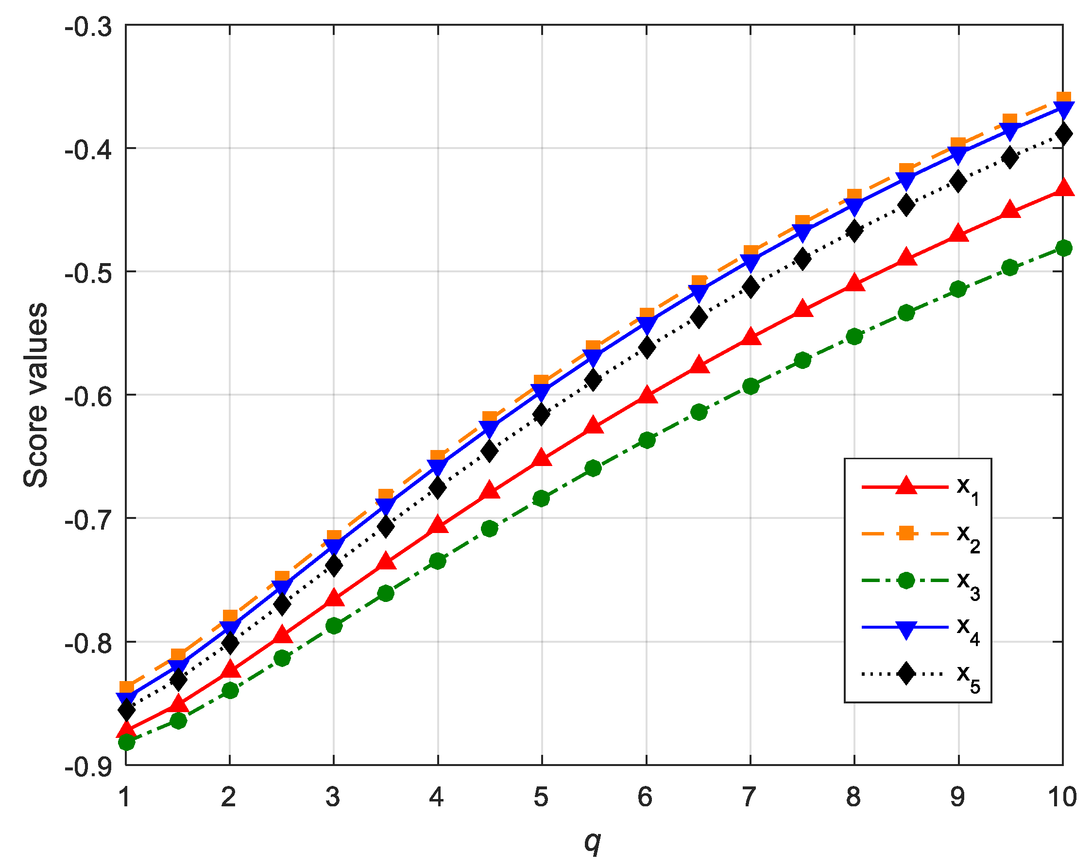
It is noted that the parameter q and the parameter vector (k₁, k₂) have great impacts on the aggregated result of alternatives in Example 3. Firstly, the influence of parameter q on aggregation results of alternatives is investigated by calculating the score functions of alternatives under the condition of parameter q taking different values. The results are presented in Figure 1.

From Figure 1, we can know that the aggregation results depend on the parameter q, the score values of alternatives $X_i$ $(i=1,2,\dots ,5)$ become greater as the parameter q increases. However, it is noted that the ranking result of alternatives is still $X_2\succ X_4\succ X_5\succ X_1\succ X_3$ no matter what values the parameter q takes. That means the parameter q is robust. The parameter q represents the space of acceptable orthopairs, that is to say, the decision maker can set an appropriate value of parameter q to model the uncertainty and fuzzy information in decision making.

In the following, under the condition of parameter vector (k₁, k₂) taking some special values, the score functions of alternatives are calculated and the calculation results are showed in

Table 6. Score values of alternatives with different values of parameter vector.

(k1, k2)	S(r1)	S(r2)	S(r3)	S(r4)	S(r5)	Ranking
(1,1)	−0.7492	−0.6960	−0.7407	−0.7036	−0.7219	$X_2\succ X_4\succ X_5\succ X_3\succ X_1$
(2,1)	−0.7497	−0.6996	−0.7473	−0.7058	−0.7224	$X_2\succ X_4\succ X_5\succ X_3\succ X_1$
(1,2)	−0.7651	−0.7113	−0.7806	−0.7201	−0.7372	$X_2\succ X_4\succ X_5\succ X_1\succ X_3$
(2,2)	−0.7657	−0.7150	−0.7874	−0.7223	−0.7377	$X_2\succ X_4\succ X_5\succ X_1\succ X_3$

.

It is known from Table 6 that the ranking order of X₂, X₄, and, X₅ remain unchanged no matter what values the parameter vector takes, whereas the ranking order of alternatives X₃ and X₁ is $X_3\succ X_1$ when the parameter vector takes (1,1) or (2,1) and the ranking order of alternatives X₃ and X₁ is $X_1\succ X_3$ when the parameter vector takes (1,2) or (2,2). The difference is due to the relationship structure of the attributes has changed when the parameter vector takes different values. The parameter vector models the types of interrelationships among attributes, therefore, a decision maker can set the appropriate values of a parameter vector to model any kind of interrelationship among attributes in decision making. Meanwhile, we can observe that the more interrelationships of attributes in each class we consider, the smaller the score values will become.

6.3. Comparative Analysis

In the following, some comparisons of the proposed approach with existing approaches are conducted to illustrate the validity and advantage of the q-ROFWPPMSM operator. We select following approaches to solve aforementioned example, including: the approach proposed by Wei and Lu [26] based on the Pythagorean fuzzy power weighted averaging (PFPWA) operators, the approach introduced by Wei and Lu [40] based on Pythagorean fuzzy weighted Maclaurin symmetric mean (PFWMSM) operator, and the approach defined by Liu et al. [16] based on intuitionistic fuzzy weighted interaction partitioned Bonferroni mean (IFWIPBM) operator. The aggregated results of the alternatives obtained by the reference approaches and the proposed approach are presented in

Table 7. Score values and ranking results by different approaches in Example 3.

Operator	Score Values of ri (i = 1, 2, 3, 4)	Ranking Result
PFPWA [26]	S(r1) = 0.5510, S(r2) = 0.6347, S(r3) = 0.5170, S(r4) = 0.6065, S(r5) = 0.5829;	$X_2\succ X_4\succ X_5\succ X_3\succ X_1$
PFWMSM [40] (Suppose k = 2)	S(r1) = 0.0914, S(r2) = 0.1135, S(r3) = 0.0919, S(r4) = 0.1091, S(r5) = 0.1029;	$X_2\succ X_4\succ X_5\succ X_3\succ X_1$
IFWIPBM [16] (Suppose p = q = 2)	S(r1) = −0.0294, S(r2) = −0.0046, S(r3) = −0.0213 S(r4) = −0.0115, S(r5) = −0.0252;	$X_2\succ X_4\succ X_3\succ X_5\succ X_1$
q-ROFWPPMSM (Suppose k1 = k2 = 2)	S(r1) = −0.7657, S(r2) = −0.7150, S(r3) = −0.7874 S(r4) = −0.7223, S(r5) = −0.7377;	$X_2\succ X_4\succ X_5\succ X_1\succ X_3$

.

It is can be observed from Table 7 that the alternatives X₂ and X₄ are respectively identified as the best alternative and second best alternative by all approaches, though the ranking orders of the rest of alternatives X₁, X₃, and, X₅ are slightly different. Thus, the validity of the proposed approach is verified.

In Example 3, the attributes are divided into two classes and the attributes of each class are interrelated to each other. In order to further demonstrate the advantage of the proposed approach, a new example with more complicated scenarios is provided and it is depicted as follows:

Example 4.

A corporation wants to select a new investment area from four alternatives $X_i$ $(i=1,2,3,4)$. After preliminary screening, there are the following five factors denoted by $C_j$ $(j=1,2,\dots ,5)$, which are selected as evaluation attributes, including: C₁: the risk of losing capital sum, C₂: the amount of interest received, C₃: the vulnerability of capital sum to modification by inflation, C₄: the market potential and, C₅: the growth potential. The corresponding attribute weight vector is $w=(0.3,0.1,0.25,0.15,0.2)$. Considering the attribute characteristics, the attributes are divided into two class P₁ = {C₁, C₂, C₃} and P₂ = {C₄, C₅}. Moreover, there is interrelationship among any three attributes in $P_1$ and there is interrelationship between any two attributes in $P_2$, that is to say, the $k_1=3$ and $k_2=2$. The evaluating values of alternatives $X_i$ $(i=1,2,3,4)$ with respect to attributes C_j are given in form of q-ROFNs and the decision matrix is present in

Table 8. The q-rung orthopair fuzzy decision matrix.

	C1	C2	C3	C4	C5
X1	(0.3, 0.6)	(0.7, 0.2)	(0.2, 0.8)	(0.8, 0.1)	(0.7, 0.3)
X2	(0.1, 0.8)	(0.8, 0.2)	(0.2, 0.6)	(0.7, 0.2)	(0.8, 0.1)
X3	(0.1, 0.85)	(0.6, 0.2)	(0.2, 0.75)	(0.8, 0.2)	(0.8, 0.2)
X4	(0.2, 0.7)	(0.9, 0.1)	(0.2, 0.7)	(0.6, 0.3)	(0.8, 0.1)

We utilize the aforementioned approaches to solve Example 4. The score value of alternatives over all attributes and ranking order obtained by different approaches are presented in

Table 9. Score values and ranking results by different approaches in Example 4.

Method	Score Values	Ranking Result
PFPWA [26]	S(r1) = 0.6708; S(r2) = 0.6949; S(r3) = 0.6710; S(r4) = 0.7086;	$X_4\succ X_2\succ X_3\succ X_1$
PFWMSM [40] (Suppose k = 2)	S(r1) = 0.2201; S(r2) = 0.2315; S(r3) = 0.2061; S(r4) = 0.2384;	$X_4\succ X_2\succ X_1\succ X_3$
IFWIPBM [16] (Suppose p = q= 1)	S(r1) = −0.5967; S(r2) = −0.4690; S(r3) = −0.3541; S(r4) = −0.3835;	$X_3\succ X_4\succ X_2\succ X_1$
q-ROFWPPMSM (Suppose k1 = 3, k2 = 2)	S(r1) = −0.4101; S(r2) = −0.3609; S(r3) = −0.4052; S(r4) = −0.4189;	$X_2\succ X_3\succ X_1\succ X_4$

.

It is known from Table 9 that the ranking order obtained by the proposed approach is significantly different from the results given by the three existing approaches. The difference is due to none of the above three approaches can exactly model the relationship structure where attributes are divided into several classes and there is interrelationship among the arguments of each class.

In the following, we compare the differences of the ranking orders of alternatives obtained by the aforementioned approaches in detail and analyze the principal cause of the above discrepancy from the perspective of the model structure.

(1)

Comparing the approach introduced by Wei and Lu [26] with the proposed approach, the alternative X₄ is respectively identified as the best alternative and worst alternative and the alternative X₂ is respectively identified as the second best alternative and the best alternative by the approach of Wei and Lu [26] and the proposed approach. The difference is due to the former only using the power aggregation operator, which can calculate the support degree between arguments whereas the later not only includes the power aggregation operation, but also considers the interrelationship among arguments. In Example 4, it is obvious that the interrelationship exists among attributes, so the proposed approach may be more reasonable than Wei and Lu’s approach [22].

(2)

Similar to the ranking order of alternatives given by the PFPWA operator, the approach of Wei and Lu [40] also respectively identified the alternatives X₄ and X₂ as the best alternative and the second best alternative, whereas the proposed approach identifies the X₄ and X₂ as the worst alternative and best alternative, respectively. The ranking order of the rest alternatives X₁ and X₃ obtained by Wei and Lu’s [40] approach and the proposed approach is $X_1\succ X_3$ and $X_3\succ X_1$, respectively. The difference is due to the approach of Wei and Lu [40], which can capture the interrelationships among attributes by using a MSM operator, which can calculate the average of the sum of satisfaction among any k attributes. However, the proposed approach considers this situation where the attributes can be divided into different classes and there is an interrelationship among any attribute in each class, whereas there is no interrelationship among attributes of any two classes.

(3)

The ranking orders obtained by the approach of Liu et al. [16] and the proposed approach are significantly different. The alternative X₃ and the alternative X₂ are respectively identified as the best alternative by the approach of Liu et al. [16] and the proposed approach. The approach of Liu et al. [16], based on the IFIPBM operator, divides attributes into different classes and assumes attributes in each class are interrelated to each other. But in Example 4, each attribute is interrelated to any other two attributes in class P₁ and each attribute in class P₂ is interrelated to each other, that is to say, the type of interrelationship of attributes in each class are different. It is obvious that the proposed approach can model the above situation better than the approach of Liu et al. [16]. Therefore the proposed approach may be more reasonable than Liu et al. [16].

7. Conclusions

In this paper, a new approach is proposed for dealing with q-rung orthopair fuzzy MAGDM problems. The contribution of this paper includes three phases. Firstly, a new aggregation operator, which is called the partitioned PMSM operator, is proposed for dealing with a situation where the attributes are divided into several parts and there is interrelationship among any attributes in each part whereas the attributes in different parts are not related. The mathematical form of the PMSM is introduced and some special cases and desirable properties of a PMSM operator are also investigated. Secondly, in order to aggregate the q-rung orthopair fuzzy information, the PMSM operator is extended in a q-ROFS and q-rung orthopair fuzzy partitioned Maclaurin symmetric mean (q-ROFPMSM) and q-rung orthopair fuzzy weighted partitioned Maclaurin symmetric mean (q-ROFWPMSM) operators are proposed. Finally, to eliminate the negative effects of unreasonable assessment values obtained by the decision maker on the decision results, we take advantage of the PA operator and propose a q-rung orthopair fuzzy power partitioned Maclaurin symmetric mean (q-ROFPPMSM) and q-rung orthopair fuzzy weighted power partitioned Maclaurin symmetric mean (q-ROFWPPMSM) operators, which combine the advantages of PMSM and PA operators. A new approach based on the q-ROFWPPMSM operator is proposed for solving q-rung orthopair fuzzy MAGDM problems. A numerical example and some comparative analysis are also conducted.

Based on the results of the comparative analysis, the main advantages of the proposed approach include: (1) the proposed PMSM can reflect the relationship structure of attributes that attributes are partitioned into several parts, and there is interrelationship among any attributes in each part; (2) the proposed PMSM can reduce MSM or PBM operator by adjusting the cardinality of set and setting different values of parameter vector; (3) the q-ROFPPMSM operator can reduce the influence of the unduly high and low arguments on ranking results. In future works, we will apply the proposed approach in other practical decision making problems, such as low carbon supplier selection, risk management, medical diagnosis, and resource evaluation, etc.

References

- Yager, R.R. The power average operator. IEEE Trans. Syst. Man Cybern. A 2001, 31, 724–731. [Google Scholar] [CrossRef]
- Bonferroni, C. Sulle medie multiple di potenze. Bolletino Matematica Italiana 1950, 5, 267–270. [Google Scholar]
- Maclaurin, C. A second letter to Martin Folkes, Esq.; Concerning the roots of equations, with demonstration of other rules of algebra. Philos. Trans. R. Soc. Lond. A 1927, 36, 59–96. [Google Scholar]
- Dutta, B.; Guha, D. Partitioned Bonferroni mean based on linguistic 2-tuple for dealing with multi-attribute group decision making. Appl. Soft Comput. 2015, 37, 166–179. [Google Scholar] [CrossRef]
- Zadeh, L.A. Fuzzy sets. Inf. Control 1965, 8, 338–356. [Google Scholar] [CrossRef]
- Merigo, J.M. Fuzzy decision making with immediate probabilities. Comput. Ind. Eng. 2010, 58, 651–657. [Google Scholar] [CrossRef]
- Merigo, J.M.; Gil-Lafuente, A.M.; Yager, R.R. An overview of fuzzy research with bibliometric indicators. Appl. Soft Comput. 2015, 27, 420–433. [Google Scholar] [CrossRef]
- Blanco-Mesa, F.; Merigo, J.M.; Gil-Lafuente, A.M. Fuzzy decision making: A bibliometric-based review. J. Intell. Fuzzy Syst. 2017, 32, 2033–2050. [Google Scholar] [CrossRef] [Green Version]
- Atanassov, K.T. Intuitionistic fuzzy sets. Fuzzy Sets Syst. 1986, 20, 87–96. [Google Scholar] [CrossRef]
- Chen, S.M.; Cheng, S.H.; Lan, T.C. A novel similarity measure between intuitionistic fuzzy sets based on the centroid points of transformed fuzzy numbers with applications to pattern recognition. Inf. Sci. 2016, 343, 15–40. [Google Scholar] [CrossRef]
- Montes, I.; Janis, V.; Pal, N.R.; Montes, S. Local divergences for Atanassov intuitionistic fuzzy sets. IEEE Trans. Fuzzy Syst. 2016, 24, 360–373. [Google Scholar] [CrossRef]
- Son, L.H.; Phong, P.H. On the performance evaluation of intuitionistic vector similarity measures for medical diagnosis. J. Intell. Fuzzy Syst. 2016, 31, 1597–1608. [Google Scholar] [CrossRef]
- Zhai, Y.; Xu, Z.; Liao, H. Measures of probabilistic interval-valued intuitionistic hesitant fuzzy sets and the application in reducing excessive medical examinations. IEEE Trans. Fuzzy Syst. 2018, 26, 1651–1670. [Google Scholar] [CrossRef]
- Wang, Z.; Xu, Z.; Liu, S.; Yao, Z. Direct clustering analysis based on intuitionistic fuzzy implication. Appl. Soft Comput. 2014, 23, 1–8. [Google Scholar] [CrossRef]
- Wang, Z.; Xu, Z.; Liu, S.; Tang, J. A netting clustering analysis method under intuitionistic fuzzy environment. Appl. Soft Comput. 2011, 11, 5558–5564. [Google Scholar] [CrossRef]
- Liu, P.; Chen, S.M.; Liu, J. Multiple attribute group decision making based on intuitionistic fuzzy interaction partitioned Bonferroni mean operators. Inf. Sci. 2017, 411, 98–121. [Google Scholar] [CrossRef]
- Liu, P. Multiple attribute decision-making methods based on normal intuitionistic fuzzy interaction aggregation operators. Symmetry 2017, 9, 261. [Google Scholar] [CrossRef]
- Liu, P.; Mahmood, T.; Khan, Q. Multi-attribute decision-making based on prioritized aggregation operator under hesitant intuitionistic fuzzy linguistic environment. Symmetry 2017, 9, 270. [Google Scholar] [CrossRef]
- Yager, R.R. Pythagorean membership grades in multi-criteria decision making. IEEE Trans. Fuzzy Syst. 2014, 22, 958–965. [Google Scholar] [CrossRef]
- Zhang, X.; Xu, Z. Extension of TOPSIS to multiple criteria decision making with Pythagorean fuzzy sets. Int. J. Intell. Syst. 2014, 29, 1061–1078. [Google Scholar] [CrossRef]
- Ren, P.; Xu, Z.; Gou, X. Pythagorean fuzzy TODIM approach to multi-criteria decision making. Appl. Soft Comput. 2016, 42, 246–259. [Google Scholar] [CrossRef]
- Zhang, X. Multicriteria Pythagorean fuzzy decision analysis: A hierarchical QUALIFLEX approach with the closeness index-based ranking methods. Inf. Sci. 2016, 30, 104–124. [Google Scholar] [CrossRef]
- Peng, X.; Yang, Y. Some results for Pythagorean fuzzy sets. Int. J. Intell. Syst. 2015, 30, 1133–1160. [Google Scholar] [CrossRef]
- Zhou, J.; Su, W.; Balezentis, T.; Streimikiene, D. Multiple criteria group decision-making considering symmetry with regards to the positive and negative ideal solutions via the Pythagorean normal cloud model for application to economic decisions. Symmetry 2018, 10, 140. [Google Scholar] [CrossRef]
- Garg, H. Generalized Pythagorean fuzzy geometric aggregation operators using Einstein t-norm and t-conorm for multicriteria decision-making process. Int. J. Intell. Syst. 2017, 32, 597–630. [Google Scholar] [CrossRef]
- Wei, G.; Lu, M. Pythagorean fuzzy power aggregation operators in multiple attribute decision making. Int. J. Intell. Syst. 2018, 33, 169–186. [Google Scholar] [CrossRef]
- Yager, R.R. Generalized orthopair fuzzy sets. IEEE Trans. Fuzzy Syst. 2017, 25, 1222–1230. [Google Scholar] [CrossRef]
- Peng, X.; Dai, J.; Garg, H. Exponential operation and aggregation operator for q-rung orthopair fuzzy set and their decision-making method with a new score function. Int. J. Intell. Syst. 2018. [Google Scholar] [CrossRef]
- Du, W.S. Minkowski-type distance measures for generalized orthopair fuzzy sets. Int. J. Intell. Syst. 2018, 33, 802–817. [Google Scholar] [CrossRef]
- Li, L.; Zhang, R.; Wang, J.; Shang, X.; Bai, K. A novel approach to multi-attribute group decision-making with q-rung picture linguistic information. Symmetry 2018, 10, 172. [Google Scholar] [CrossRef]
- Liu, P.; Wang, P. Some q-rung orthopair fuzzy aggregation operators and their applications to multiple-attribute decision making. Int. J. Intell. Syst. 2018, 33, 259–280. [Google Scholar] [CrossRef]
- Liu, P.; Liu, J. Some q-rung orthopai fuzzy Bonferroni mean operators and their application to multi-attribute group decision making. Int. J. Intell. Syst. 2018, 33, 315–347. [Google Scholar] [CrossRef]
- Wei, G.; Gao, H.; Wei, Y. Some q-rung orthopair fuzzy Heronian mean operators in multiple attribute decision making. Int. J. Intell. Syst. 2018, 33, 1426–1458. [Google Scholar] [CrossRef]
- Liu, P.; Wang, P. Multiple-attribute decision-making based on Archimedean Bonferroni Operators of q-rung orthopair fuzzy numbers. IEEE Trans. Fuzzy Syst. 2018. [Google Scholar] [CrossRef]
- Xu, Z.; Yager, R.R. Power-geometric operators and their use in group decision making. IEEE Trans. Fuzzy Syst. 2010, 18, 94–105. [Google Scholar]
- Yager, R.R. On generalized Bonferroni mean operators for multi-criteria aggregation. Int. J. Approx. Reason 2009, 50, 1279–1286. [Google Scholar] [CrossRef]
- Xia, M.; Xu, Z.; Zhu, B. Generalized intuitionistic fuzzy Bonferroni means. Int. J. Intell. Syst. 2012, 27, 23–47. [Google Scholar] [CrossRef]
- Zhang, R.; Wang, J.; Zhu, X.; Xia, M.; Yu, M. Some generalized Pythagorean fuzzy Bonferroni mean aggregation operators with their application to multi-attribute group decision-making. Complexity 2017, 2017, 1–16. [Google Scholar]
- Detemple, D.; Robertson, J. On generalized symmetric means of two variables. Publikacije Elektrotehničkog fakulteta. Serija Matematika I Fizika 1979, 677, 236–238. [Google Scholar]
- Wei, G.; Lu, M. Pythagorean fuzzy Maclaurin symmetric mean operators in multiple attribute decision making. Int. J. Intell. Syst. 2018, 33, 1043–1070. [Google Scholar] [CrossRef]
- Ju, Y.; Liu, X.; Ju, D. Some new intuitionistic linguistic aggregation operators based on Maclaurin symmetric mean and their applications to multiple attribute group decision making. Soft Comput. 2016, 20, 4521–4548. [Google Scholar] [CrossRef]
- Liu, P.; Gao, H. Multicriteria decision making based on generalized Maclaurin symmetric means with multi-hesitant fuzzy linguistic information. Symmetry 2018, 10, 81. [Google Scholar] [CrossRef]
- Liu, P.; Liu, J.; Merigo, J.M. Partitioned Heronian means based on linguistic intuitionistic fuzzy numbers for dealing with multi-attribute group decision making. Appl. Soft Comput. 2018, 62, 395–422. [Google Scholar] [CrossRef]
- Liu, Z.; Liu, P. Intuitionistic uncertain linguistic partitioned Bonferroni means and their application to multiple attribute decision-making. Int. J. Syst. Sci. 2017, 48, 1092–1105. [Google Scholar] [CrossRef]
- Liu, Z.; Liu, P.; Liu, W.; Pang, J. Pythagorean uncertain linguistic partitioned Bonferroni mean operators and their application in multi-attribute decision making. J. Intell. Fuzzy Syst. 2017, 32, 2779–2790. [Google Scholar] [CrossRef]
Figure 1.
Score values of the alternatives Xi when .