The Absolute Ruin Insurance Risk Model with a Threshold Dividend Strategy

Abstract

The absolute ruin insurance risk model is modified by including some valuable market economic information factors, such as credit interest, debit interest and dividend payments. Such information is especially important for insurance companies to control risks. We further assume that the insurance company is able to finance and continue to operate when its reserve is negative. We investigate the integro-differential equations for some interest actuarial diagnostics. We also provide numerical examples to explain the effects of relevant parameters on actuarial diagnostics.

1. Introduction

Consider the classical insurance risk model, the cash flow of company is modeled by the risk reserve process $\{R_t^u;t\ge 0\}$, with

$$\begin{array}{c}\hfill R_t^u=u+pt-S(t),t\ge 0.\end{array}$$

(1)

Here, $R_0^u=u\ge 0$ denotes the initial reserve, and $p>0$ denotes the premium density which is assumed to be constant. $S(t)={\sum }_{k=1}^{N_t}{Y}_k$, representing the aggregate claim process, is a compound Poisson process, given by a Poisson rate $\lambda >0$, $\{Y_k;k=1,2,\dots \}$ that represents the claim size process and is independent of the Poisson process $\{N_t;t\ge 0\}$ which are i.i.d. random variables with the distribution function $G(y)$ and mean $\mu >0$. In the present paper, in order to make the risk model closer to the actual operating situation, we added three other properties related to the risk reserve process (1), namely, debit interest, credit interest and dividend payments. In particular, we made a distinction between ruin and absolute ruin. That is, the insurance company can borrow money and continue to operate when the company’s reserve is negative.

It should be mentioned that many authors have studied the problems of absolute ruin, for example, Cai [1] studied the Gerber-Shiu function in the case of absolute ruin. Wang and Yin [2] investigated the absolute ruin model with barrier strategy. Wang et al. [3], Yuan et al. [4] and Peng et al. [5] extended the work of Wang and Yin [2], and studied interest income with the barrier strategy. Wang et al. [6] further considered a threshold dividend barrier under the absolute ruin risk model. Li and Lu [7] further explored the case of the Markov-dependent risk model under absolute ruin. The advantage of this Markov-dependent risk model is that different economic conditions can be expressed by different states of Markov chains. Such models can better cope with changes in the economic environment. For more recent studies about absolute ruin problems, see Huu et al. [8], Luo and Taksar [9], Yang et al. [10,11], Yu [12], Cai and Yang [13], Zhu [14,15], Bi and Zhang [16], Liu and Yang [17], Zeng and Li [18], Zeng et al. [19], Peng and Wang [20,21] and Avram et al. [22].

Motivated by the above literature, in our model, we divided the risk reserve process into three cases according to the size of the reserve. When the risk reserve is between zero and a fixed level ($b>0$), the premium income rate is $p_1$, at which interest is not earnt and no dividends are paid. When the risk reserve attains the level b, its interest at a credit interest rate of $\gamma >0$ and moreover dividends are paid to shareholders continuously at a certain rate $\epsilon (0<\epsilon \le p_1)$. The premium income rate at this time is $p_2=p_1-\epsilon$. When the risk reserve is at a negative value, the company is able to finance at a debit interest rate $\beta >0$ and carry on their business operations.

By incorporating the above-mentioned three features into the reserve process $\{R_t^u;t\ge 0\}$ of (1), the new resulting risk reserve process $\{R_t^{u,b};t\ge 0\}$ is given by the following equations

$$\begin{array}{c}\hfill d{R}_t^{u,b}=\left\{\begin{array}{c}(p_2+\gamma R_t^{u,b})dt-dS(t),R_t^{u,b}>b,\hfill \\ p_{1}dt-dS(t),0\le R_t^{u,b}\le b,\hfill \\ (p_1+\beta R_t^{u,b})dt-dS(t),-p_1/R_t^{u,b}\le 0.\hfill \end{array}\right.\end{array}$$

(2)

Here, $R_0^{u,b}=u$, ${\displaystyle S(t)=\sum _{k=1}^{N_t}{Y}_k}$ is defined in model (1).

Let us denote the set $T_b=\inf \{t\ge 0|R_t^{u,b}\le -p_1/\beta \}$ by $T_b$ with $T_b=\infty$ if $R_t^{u,b}>-p_1/\beta$ for all $t\ge 0$, and name it the time of absolute ruin. $\alpha (\alpha >0)$ is defined as the force of interest, and $D(t)$ is the accumulated value of all dividends payable until t time. Then, the present value of all dividends until absolute ruin time is given by

$$\begin{array}{c}\hfill D_{u,b}={\int }_0^{T_b}{e}^{-\alpha t}dD(t)=\epsilon {\int }_0^{T_b}{e}^{-\alpha t}I(R_t^{u,b}>b)dt.\end{array}$$

(3)

Here, $I(·)$ denotes the indicator function. It is worth noting that $D_{u,b}$ satisfies ${\displaystyle 0<D_{u,b}\le \epsilon {\int }_0^{+\infty }{e}^{-\alpha t}dt=\epsilon /\alpha }$.

Next, we focused on the following four related actuarial functions of $D_{u,b}$.

The moment generating function of $D_{u,b}$ is

$$\begin{array}{c}\hfill Q(u,z;b)=E[e^{z{D}_{u,b}}],\end{array}$$

(4)

for some values of z where it exists.

The nth moment function of $D_{u,b}$ is

$$\begin{array}{c}\hfill W_n(u;b)=E\{{[D_{u,b}]}^n]\},n\in N,\end{array}$$

(5)

with $W_0(u;b)=1$.

The Laplace transform of absolute ruin time ($\rho$ is a positive constant) is

$$\begin{array}{c}\hfill \phi (u;b)=E[e^{-\rho T_b}I(T_b<\infty )|R_0^{u,b}=u].\end{array}$$

(6)

The Gerber-Shiu expected discounted penalty function is

$$\begin{array}{c}\hfill \mathrm{\Phi }(u;b)=E[e^{-\alpha T_b}\omega (R_{T_b-}^{u,b},|R_{T_b}^{u,b}|)I(T_b<\infty )|R_0^{u,b}=u],\end{array}$$

(7)

where, $R_{T_b-}^{u,b}$ is the instantaneous reserve before absolute ruin time. $|R_{T_b}^{u,b}|$ is the deficit at absolute ruin time. $\omega (x_1,x_2)$ is a measurable function defined on $(-p_1/\beta ,+\infty )\times (p_1/\beta ,+\infty )$ that can be interpreted as a penalty at the time of absolute ruin.

2. Integro-Differential Equations for $\mathit{Q}(\mathit{u},\mathit{z};\mathit{b})$ and ${\mathit{W}}_{\mathit{n}}(\mathit{u};\mathit{b})$

In the sections below, we first give a system of partial integro-differential equations satisfied by $Q(u,z;b)$, through which we can further analyze the $W_n(u;b)$. Note that $Q(u,z;b)$ has different expressions according to the different values of u. Hence, we discuss it for three cases by writing $Q(u,z;b)=Q_1(u,z;b)$ for $0\le u\le b$, $Q(u,z;b)=Q_2(u,z;b)$ for $u>b$, and $Q(u,z;b)=Q_3(u,z;b)$ for $-p_1/\beta <u<0$. For convenience of the following proof, we set

$$\begin{array}{c}\hfill h_1(u,t)=u{e}^{\beta t}+p_1(e^{\beta t}-1)/\beta ,h_2(u,t)=u{e}^{\gamma t}+p_2(e^{\gamma t}-1)/\gamma .\end{array}$$

(8)

Theorem 1.

When $0\le u\le b$,

$$\begin{array}{cc}\hfill p_1\frac{\partial Q_1(u,z;b)}{\partial u}=& \lambda Q_1(u,z;b)+\alpha z\frac{\partial Q_1(u,z;b)}{\partial z}-\lambda \left[{\int }_0^u{Q}_1(u-y,z;b)dG(y)\right.\hfill \\ & \left.+{\int }_u^{u+p_1/\beta }{Q}_3(u-y,z;b)dG(y)+\overline{G}(u+\frac{p_1}{\beta })\right],\hfill \end{array}$$

(9)

and, when $u>b$,

$$\begin{array}{cc}\hfill (\gamma u+p_2)\frac{\partial Q_2(u,z;b)}{\partial u}=& \lambda Q_2(u,z;b)+\alpha z\frac{\partial Q_2(u,z;b)}{\partial z}-\lambda \left[{\int }_0^{u-b}{Q}_2(u-y,z;b)dG(y)\right.\hfill \\ & +{\int }_{u-b}^u{Q}_1(u-y,z;b)dG(y)+{\int }_u^{u+p_1/\beta }{Q}_3(u-y,z;b)dG(y),\hfill \\ & \left.+\overline{G}(u+\frac{p_1}{\beta })\right]\hfill \end{array}$$

(10)

and, when $-p_1/\beta <u<0$,

$$\begin{array}{cc}\hfill (\beta u+p_1)\frac{\partial Q_3(u,z;b)}{\partial u}=& \lambda Q_3(u,z;b)+\alpha z\frac{\partial Q_3(u,z;b)}{\partial z}\hfill \\ & -\lambda \left[{\int }_0^{u+p_1/\beta }{Q}_3(u-y,z;b)dG(y)+\overline{G}(u+\frac{p_1}{\beta })\right].\hfill \end{array}$$

(11)

Proof. 

(1)

For $0\le u\le b$, as discussed in Albrecher et al. [23], and using the strong Markov property of the risk reserve process $\{R_t^{u,b},t\ge 0\}$, we obtain

$$\begin{array}{cc}\hfill Q_1(u,z;b)=& (1-\lambda t)Q_1(u+p_{1}t,z{e}^{-\alpha t};b)\hfill \\ & +\lambda t·\left[{\int }_0^{u+p_{1}t}{Q}_1(u+p_{1}t-y,z{e}^{-\alpha t};b)dG(y)\right.\hfill \\ & \left.+{\int }_{u+p_{1}t}^{u+p_{1}t+\frac{p_1}{\beta }}{Q}_3(u+p_{1}t-y,z{e}^{-\alpha t};b)dG(y)+\overline{G}(u+p_{1}t+\frac{p_1}{\beta })\right]+o(t),\hfill \end{array}$$

(12)

where, $O(t)$ is the high order infinitesimal of t when $t\to 0$, i.e., ${\displaystyle \underset{t\to 0}{\lim }\frac{O(t)}{t}=0}$.

By Taylor expansion,

$$\begin{array}{cc}\hfill Q_1(u+p_{1}t,z{e}^{-\alpha t};b)=& Q_1(u,z;b)+p_{1}t\frac{\partial Q_1(u,z;b)}{\partial u}-\alpha zt\frac{\partial Q_1(u,z;b)}{\partial z}+o(t).\hfill \end{array}$$

(13)

By plugging (13) into (12), we can obtain (9).

(2)

The above method is applied to $Q_2(u,z;b)$ when $u>b$, and we have

$$\begin{array}{cc}\hfill Q_2(u,z;b)=& (1-\lambda t)·Q_2(h_2(u,t),z{e}^{-\alpha t};b)+\lambda t·\left[{\int }_0^{h_2(u,t)-b}{Q}_2(h_2(u,t)-y,z{e}^{-\alpha t};b)dG(y)\right.\hfill \\ & +{\int }_{h_2(u,t)-b}^{h_2(u,t)}{Q}_1(h_2(u,t)-y,z{e}^{-\alpha t};b)dG(y)\hfill \\ & +{\int }_{h_2(u,t)}^{h_2(u,t)+\frac{p_1}{\beta }}{Q}_3(h_2(u,t)-y,z{e}^{-\alpha t};b)dG(y)\hfill \\ & \left.+\overline{G}(h_2(u,t)+\frac{p_1}{\beta })\right]+o(t).\hfill \end{array}$$

(14)

By Taylor expansion,

$$\begin{array}{cc}\hfill Q_2(h_2(u,t),z{e}^{-\alpha t};b)=& Q_2(u,z;b)+(\gamma u+p_2)t\frac{\partial Q_2(u,z;b)}{\partial u}\hfill \\ & -\alpha zt\frac{\partial Q_2(u,z;b)}{\partial z}+o(t).\hfill \end{array}$$

(15)

By plugging (15) into (14), we have (10).

(3)

For $-p_1/\beta <u<0$, the same argument as in the proof of (10) gives

$$\begin{array}{cc}\hfill Q_3(u,z;b)=& (1-\lambda t)·Q_3(h_1(u,t),z{e}^{-\alpha t};b)\hfill \\ & +\lambda t·\left[{\int }_0^{h_1(u,t)+\frac{p_1}{\beta }}{Q}_3(h_1(u,t)-y,z{e}^{-\alpha t};b)dG(y)\right.\hfill \\ & \left.+\overline{G}(h_1(u,t)+\frac{p_1}{\beta })\right]+o(t).\hfill \end{array}$$

(16)

By Taylor expansion, we have (11). ☐

Theorem 2.

$Q_1(u,z;b)$, $Q_2(u,z;b)$ and $Q_3(u,z;b)$ satisfy

$$\begin{array}{c}\hfill Q_3(-\frac{p_1}{\beta },z;b)=1,\end{array}$$

(17)

$$\begin{array}{c}\hfill \frac{\partial Q_1(u,z;b)}{\partial u}{|}_{u=b}=y{Q}_1(b,z;b),\end{array}$$

(18)

$$\begin{array}{c}\hfill Q_1(b-,z;b)=Q_2(b+,z;b),\end{array}$$

(19)

$$\begin{array}{c}\hfill Q_1(0+,z;b)=Q_3(0-,z;b).\end{array}$$

(20)

Proof. 

(1)

For (17), if ${\displaystyle u=-\frac{p_1}{\beta }}$, it is obvious that the absolute ruin will happen immediately, and no dividend is paid, which implies (17).

(2)

For (18), when $u=b$, we have

$$\begin{array}{cc}\hfill Q_1(b,z;b)=& (1-\lambda t)e^{p_{1}t}{Q}_1(b,z{e}^{-\alpha t};b)+\lambda t·\left[{\int }_0^b{Q}_1(b-y,z{e}^{-\alpha t};b)dG(y)\right.\hfill \\ & \left.+{\int }_b^{b+\frac{p_1}{\beta }}{Q}_2(b-y,z{e}^{-\alpha t};b)dG(y)+\overline{G}(b+\frac{p_1}{\beta })\right]+o(t).\hfill \end{array}$$

(21)

By plugging $u=b$ into (9) and using (21), we obtain (18).

(3)

For (19) and (20), the method is analogous to Wan [24], so we leave it out here.

Let us now consider the problem of $W_n(u,b)$. Following the same argument as above according to the different initial reserves, $W_n(u,b)$ is a piecewise function. We denote

$$\begin{array}{c}\hfill W_n(u;b)=\left\{\begin{array}{c}{W}_{n2}(u;b),u>b,\hfill \\ W_{n1}(u;b),0\le u\le b,\hfill \\ W_{n3}(u;b),-p_1/\beta <u<0,\hfill \end{array}\right.\end{array}$$

(22)

where $W_{01}(b;b)=1$.

According to the representation theorem, we have

$$\begin{array}{c}\hfill Q_i(u,z;b)=1+\sum _{n=1}^{\infty }\frac{z^n}{n!}{W}_{ni}(u;b),i=1,2,3,n\in N^{+},\end{array}$$

(23)

and equating the coefficients of $z^n$ in (9)–(11), we can show that $W_{ni}(u;b)(i=1,2,3.)$ satisfies the following integro-differential equations and corresponding boundary conditions. ☐

Theorem 3.

When $0\le u\le b$,

$$\begin{array}{cc}\hfill p_1{W}_{n1}^{\prime }(u;b)=& (\lambda +n\alpha )W_{n1}(u;b)-\lambda \left[{\int }_0^u{W}_{n1}(u-y;b)dG(y)\right.\hfill \\ & \left.+{\int }_u^{u+p_1/\beta }{W}_{n3}(u-y;b)dG(y)\right],\hfill \end{array}$$

(24)

and when $u>b$,

$$\begin{array}{cc}\hfill (\gamma u+p_2)W_{n2}^{\prime }(u;b)=& (\lambda +n\alpha )W_{n2}(u;b)-\lambda \left[{\int }_0^{u-b}{W}_{n2}(u-y;b)dG(y)\right.\hfill \\ & \left.+{\int }_{u-b}^u{W}_{n1}(u-y;b)dG(y)+{\int }_u^{u+p_1/\beta }{W}_{n3}(u-y;b)dG(y)\right],\hfill \end{array}$$

(25)

and when $-p_1/\beta <u<0$,

$$\begin{array}{cc}\hfill (\beta u+p_1)W_{n3}^{\prime }(u;b)=& (\lambda +n\alpha )W_{n3}(u;b)-\lambda {\int }_0^{u+p_1/\beta }{W}_{n3}(u-y;b)dG(y),\hfill \end{array}$$

(26)

with boundary conditions

$$\begin{array}{c}\hfill W_{n3}(-p_1/\beta ;b)=0,\end{array}$$

(27)

$$\begin{array}{c}\hfill W_{n1}^{\prime }{(u;b)|}_{u=b}=n{W}_{n-1,1}(b;b),\end{array}$$

(28)

$$\begin{array}{c}\hfill W_{n1}(0+;b)=W_{n3}(0-;b),\end{array}$$

(29)

$$\begin{array}{c}\hfill W_{n1}(b-;b)=W_{n2}(b+;b),\end{array}$$

(30)

$$\begin{array}{c}\hfill W_{n1}^{\prime }(0+;b)=W_{n3}^{\prime }(0-;b),\end{array}$$

(31)

$$\begin{array}{c}\hfill p_1{W}_{n1}^{\prime }(b-;b)=(\gamma b+p_2)W_{n2}^{\prime }(b+;b),\end{array}$$

(32)

where $N^{+}$ represents non-negative integers.

3. Explicit Expressions for Exponential Claims to ${\mathit{W}}_{\mathit{n}}(\mathit{u};\mathit{b})$ and Numerical Examples

We suppose that claim sizes obey an exponential distribution with mean $\mu >0$. Then, Equations (24)–(26) are reduced to

$$\begin{array}{cc}\hfill p_1{W}_{n1}^{\prime }(u;b)=& (\lambda +n\alpha )W_{n1}(u;b)-\frac{\lambda }{\mu }{e}^{-\frac{u}{\mu }}\left[{\int }_0^u{W}_{n1}(y;b)e^{\frac{y}{\mu }}dy+{\int }_{-p_1/\beta }^0{W}_{n3}(y;b)e^{\frac{y}{\mu }}dy\right],\hfill \\ & 0\le u\le b,\hfill \end{array}$$

(33)

$$\begin{array}{cc}\hfill (\gamma u+p_2)W_{n2}^{\prime }(u;b)=& (\lambda +n\alpha )W_{n2}(u;b)-\frac{\lambda }{\mu }{e}^{-\frac{u}{\mu }}\left[{\int }_0^u{W}_{n2}(y;b)e^{\frac{y}{\mu }}dy\right.\hfill \\ & \left.+{\int }_0^b{W}_{n1}(y;b)e^{\frac{y}{\mu }}dy+{\int }_{-p_1/\beta }^0{W}_{n3}(y;b)e^{\frac{y}{\mu }}dy\right],u>b,\hfill \end{array}$$

(34)

$$\begin{array}{c}\hfill (\beta u+p_1)W_{n3}^{\prime }(u;b)=(\lambda +n\alpha )W_{n3}(u;b)-\frac{\lambda }{\mu }{e}^{-\frac{u}{\mu }}{\int }_{-p_1/\beta }^u{W}_{n3}(y;b)e^{\frac{y}{\mu }}dy,-p_1/\beta <u\le 0.\end{array}$$

(35)

By applying the operator $\left({\displaystyle \frac{d}{du}+\frac{1}{\mu }}\right)$ on (33)–(35), respectively, and then rearranging them, we yield

$$\begin{array}{c}\hfill W_{n1}^{{}^{″}}(u;b)+\left(\frac{1}{\mu }-\frac{\lambda +n\alpha }{p_1}\right)W_{n1}^{{}^{\prime }}(u;b)-\frac{n\alpha }{\mu p_1}{W}_{n1}(u;b)=0,0\le u\le b,\end{array}$$

(36)

$$\begin{array}{c}\hfill (\gamma u+p_2)W_{n2}^{{}^{″}}(u;b)+\left(\frac{\gamma u+p_2}{\mu }+\gamma -(\lambda +n\alpha )\right)W_{n2}^{{}^{\prime }}(u;b)-\frac{n\alpha }{\mu }{W}_{n2}(u;b)=0,u>b,\end{array}$$

(37)

$$\begin{array}{c}\hfill (\beta u+p_1)W_{n3}^{{}^{″}}(u;b)+\left(\frac{\beta u+p_1}{\mu }+\beta -(\lambda +n\alpha )\right)W_{n3}^{{}^{\prime }}(u;b)-\frac{n\alpha }{\mu }{W}_{n3}(u;b)=0,\\ \hfill -p_1/\beta <u\le 0.\end{array}$$

(38)

Obviously, the general solution of Equation (36) can be expressed as

$$\begin{array}{c}\hfill W_{n1}(u;b)={\xi }_{n1}{e}^{{\delta }_{n1}u}+{\xi }_{n2}{e}^{{\delta }_{n2}u},0\le u\le b,\end{array}$$

(39)

where ${\xi }_{n1}$ and ${\xi }_{n3}$ are arbitrary constants, and ${\delta }_{n1}$ and ${\delta }_{n2}$ are the two real roots of the following equation

$$\begin{array}{c}\hfill {\delta }^2+{\varsigma }_{1n}\delta +{\varsigma }_{2n}=0,\end{array}$$

(40)

with ${\displaystyle {\varsigma }_{1n}=\frac{1}{\mu }-\frac{\lambda +n\alpha }{p_1}}$, ${\displaystyle {\varsigma }_{2n}=\frac{-n\alpha }{\mu p_1}}$ satisfying ${\varsigma }_{1n}^2-4{\varsigma }_{2n}>0$, i.e.,

$$\begin{array}{c}\hfill {\delta }_{n1}=\frac{-{\varsigma }_{1n}+\sqrt{{\varsigma }_{1n}^2-4{\varsigma }_{2n}}}{2},{\delta }_{n2}=\frac{-{\varsigma }_{1n}-\sqrt{{\varsigma }_{1n}^2-4{\varsigma }_{2n}}}{2}.\end{array}$$

(41)

Equations similar to (37) and (38) can be found in Paulsen and Gjessing [25] and Cai and Yang [26]. By introducing the new variables, ${\displaystyle x=-\frac{\gamma u+p_2}{\gamma \mu }}$ for $u>b$ and ${\displaystyle z=-\frac{\beta u+p_1}{\beta \mu }}$ for $-p_1/\beta <u\le 0$, and letting $W_{n2}(u,b)=g_n(x)$ and $W_{n3}(u,b)=f_n(z)$, Equations (37) and (38) can be converted into Kummer’s confluent hypergeometric equation (see Salter [27] and Seaborn [28]) for functions $g_n(x)$ and $f_n(z)$:

$$\begin{array}{c}\hfill x{g}_n^{″}(x)+\left(1-\frac{\lambda +n\alpha }{\gamma }-y\right)g_n^{\prime }(x)-\frac{n\alpha }{\gamma }{g}_n(x)=0,-\frac{p_2}{\gamma \mu }<x<0,\end{array}$$

(42)

$$\begin{array}{c}\hfill z{f}_n^{″}(z)+\left(1-\frac{\lambda +n\alpha }{\beta }-z\right)f_n^{\prime }(z)-\frac{n\alpha }{\beta }{f}_n(z)=0,-\frac{p_1}{\beta \mu }<z<0.\end{array}$$

(43)

Using the solutions of (42) and (43), we conclude that

$$\begin{array}{c}\hfill W_{n2}(u;b)=g_n(x)={\xi }_{n3}{\eta }_{n3}(u)+{\xi }_{n4}{\eta }_{n4}(u),u>b,\end{array}$$

(44)

$$\begin{array}{c}\hfill W_{n3}(u;b)=f_n(x)={\xi }_{n5}{\eta }_{n5}(u)+{\xi }_{n6}{\eta }_{n6}(u),-p_1/\beta <u\le 0,\end{array}$$

(45)

where, ${\xi }_{n3}$, ${\xi }_{n4}$, ${\xi }_{n5}$ and ${\xi }_{n6}$ are arbitrary constants, and

$$\begin{array}{cc}\hfill {\eta }_{n3}(u)& =\exp \{-\frac{\gamma u+p_2}{\gamma \mu }\}·U\left(1-\frac{\lambda }{\gamma },1-\frac{\lambda +n\alpha }{\gamma };\frac{\gamma u+p_2}{\gamma \mu }\right),\hfill \\ \hfill {\eta }_{n4}(u)& ={\left(\frac{\gamma u+p_2}{\gamma \mu }\right)}^{(\lambda +n\alpha )/\gamma }·\exp \{-\frac{\gamma u+p_2}{\gamma \mu }\}·M\left(1+\frac{n\alpha }{\gamma },1+\frac{\lambda +n\alpha }{\gamma };\frac{\gamma u+p_2}{\gamma \mu }\right),\hfill \\ \hfill {\eta }_{n5}(u)& =\exp \{-\frac{\beta u+p_1}{\beta \mu }\}·U\left(1-\frac{\lambda }{\beta },1-\frac{\lambda +n\alpha }{\beta };\frac{\beta u+p_1}{\beta \mu }\right),\hfill \\ \hfill {\eta }_{n6}(u)& ={\left(\frac{\beta u+p_1}{\beta \mu }\right)}^{(\lambda +n\alpha )/\beta }·\exp \{-\frac{\beta u+p_1}{\beta \mu }\}·M\left(1+\frac{n\alpha }{\beta },1+\frac{\lambda +n\alpha }{\beta };\frac{\beta u+p_1}{\beta \mu }\right),\hfill \\ \hfill M(a_1,a_2;x)& =\frac{\Gamma (a_2)}{\Gamma (a_2-a_1)\Gamma (a_1)}{\int }_0^1{e}^{xt}{t}^{a_1-1}{(1-t)}^{a_2-a_1-1}dt,a_2>a_1>0,\hfill \\ \hfill U(a_1,a_2;x)& =\frac{1}{\Gamma (a_1)}{\int }_0^{\infty }{e}^{-xt}{t}^{a_1-1}{(1+t)}^{a_2-a_1-1}dt,y>0,a_1>0.\hfill \end{array}$$

Using the confluent hypergeometric function property, if $\beta \ne \lambda +n\alpha$, we get

$$\begin{array}{c}\hfill \underset{u\downarrow -\frac{p_1}{\beta }}{\lim }{\eta }_{n5}(u)=\Gamma \left({\displaystyle \frac{\lambda +n\alpha }{\beta }}\right)/\Gamma \left({\displaystyle \frac{\beta +n\alpha }{\beta }}\right),\underset{u\downarrow -\frac{p_1}{\beta }}{\lim }{\eta }_{n6}(u)=0,\end{array}$$

(46)

where ↓ denotes a decreasing approach. Letting ${\displaystyle u\downarrow -\frac{p_1}{\beta }}$ in (45) on both sides and together with (45), (46) and (27), we see that ${\xi }_{n5}=0$, which means that for ${\displaystyle -\frac{p_1}{\beta }<u<0}$,

$$\begin{array}{c}\hfill V_{n3}(u;b)={\xi }_{n6}{\eta }_{n6}(u).\end{array}$$

(47)

Next, we give the explicit values of ${\xi }_{n1},{\xi }_{n2},{\xi }_{n3},{\xi }_{n4},{\xi }_{n6}({\xi }_{n5}=0)$ for $n=1$ and $n\ge 2$.

When $n=1$, according to (28)–(32), (39), (44) and (47), we have

$$\begin{array}{c}\hfill \left\{\begin{array}{c}{\xi }_{11}{\delta }_{11}{e}^{{\delta }_{11}b}+{\xi }_{12}{\delta }_{12}{e}^{{\delta }_{12}b}=1,\hfill \\ {\xi }_{11}+{\xi }_{12}={\xi }_{16}{\eta }_{16}(0),\hfill \\ {\xi }_{11}{\delta }_{11}+{\xi }_{12}{\delta }_{12}={\xi }_{16}{\eta }_{16}^{\prime }(0),\hfill \\ {\xi }_{11}{e}^{{\delta }_{11}b}+{\xi }_{12}{e}^{{\delta }_{12}b}={\xi }_{13}{\eta }_{13}(b)+{\xi }_{14}{\eta }_{14}(b),\hfill \\ p_1({\xi }_{11}{\delta }_{11}{e}^{{\delta }_{11}b}+{\xi }_{12}{\delta }_{12}{e}^{{\delta }_{12}b})=(\gamma b+p_2)[{\xi }_{13}{\eta }_{13}^{\prime }(b)+{\xi }_{14}{\eta }_{14}^{\prime }(b)].\hfill \end{array}\right.\end{array}$$

(48)

By solving the above equations (48), we obtain

$$\begin{array}{c}\hfill \left\{\begin{array}{cc}{\xi }_{11}\hfill & {\displaystyle =\frac{{\eta }_{16}^{\prime }(0)-{\delta }_{12}{\eta }_{16}(0)}{{\delta }_{11}{e}^{{\delta }_{11}b}[{\eta }_{16}^{\prime }(0)-{\delta }_{12}{\eta }_{16}(0)]+{\delta }_{12}{e}^{{\delta }_{12}b}[{\delta }_{11}{\eta }_{16}(0)-{\eta }_{16}^{\prime }(b)]},}\hfill \\ {\xi }_{12}\hfill & {\displaystyle =\frac{{\delta }_{11}{\eta }_{16}(0)-{\eta }_{16}^{\prime }(0)}{{\delta }_{11}{e}^{{\delta }_{11}b}[{\eta }_{16}^{\prime }(0)-{\delta }_{12}{\eta }_{16}(0)]+{\delta }_{12}{e}^{{\delta }_{12}b}[{\delta }_{11}{\eta }_{16}(0)-{\eta }_{16}^{\prime }(b)]},}\hfill \\ {\xi }_{13}\hfill & {\displaystyle =\frac{1}{{\eta }_{13}(b)}\{{\theta }_1-{\eta }_{14}(b)\frac{(\gamma b+p_2){\eta }_{13}^{\prime }(b)){\theta }_1-{\eta }_{13}(b)p_1}{(\gamma b+p_2)[{\eta }_{13}^{\prime }(b){\eta }_{14}(b)-{\eta }_{13}(b){\eta }_{14}^{\prime }(b)]}\},}\hfill \\ {\xi }_{14}\hfill & {\displaystyle =\frac{(\gamma b+p_2){\eta }_{13}^{\prime }(b){\theta }_1-{\eta }_{13}(b)p_1}{(\gamma b+p_2)[{\eta }_{13}^{\prime }(b){\eta }_{14}(b)-{\eta }_{13}(b){\eta }_{14}^{\prime }(b)]},}\hfill \\ {\xi }_{16}\hfill & {\displaystyle =\frac{{\delta }_{11}-{\delta }_{12}}{{\delta }_{11}{e}^{{\delta }_{11}b}[{\eta }_{16}^{\prime }(0)-{\delta }_{12}{\eta }_{16}(0)]+{\delta }_{12}{e}^{{\delta }_{12}b}[{\delta }_{11}{\eta }_{16}(0)-{\eta }_{16}^{\prime }(b)]},}\hfill \end{array}\right.\end{array}$$

where ${\delta }_{11}$ and ${\delta }_{12}$ are given by (41) in the case of $n=1$, and

$$\begin{array}{c}\hfill {\displaystyle {\theta }_1=\frac{e^{{\delta }_{11}b}[{\eta }_{16}^{\prime }(0)-{\delta }_{12}{\eta }_{16}(0)]+e^{{\delta }_{12}b}[{\delta }_{11}{\eta }_{16}(0)-{\eta }_{16}^{\prime }(0)]}{{\delta }_{11}{e}^{{\delta }_{11}b}[{\eta }_{16}^{\prime }(0)-{\delta }_{12}{\eta }_{16}(0)]+{\delta }_{12}{e}^{{\delta }_{12}b}[{\delta }_{11}{\eta }_{16}(0)-{\eta }_{16}^{\prime }(0)]}.}\end{array}$$

Therefore, we arrive at the explicit expressions for $W_{11}(u;b)$, $W_{12}(u;b)$ and $W_{13}(u;b)$, namely,

$$\begin{array}{c}\hfill {\displaystyle W_{11}(u;b)=\frac{[{\eta }_{16}^{{}^{\prime }}(0)-{\delta }_{12}{\eta }_{16}(0)]e^{{\delta }_{11}u}+[{\delta }_{11}{\eta }_{16}(0)-{\eta }_{16}^{{}^{\prime }}(0)]e^{{\delta }_{12}u}}{{\delta }_{11}{e}^{{\delta }_{11}b}[{\eta }_{16}^{{}^{\prime }}(0)-{\delta }_{12}{\eta }_{16}(0)]+{\delta }_{12}{e}^{{\delta }_{12}b}[{\delta }_{11}{\eta }_{16}(0)-{\eta }_{16}^{{}^{\prime }}(0)]},0\le u\le b,}\end{array}$$

(49)

$$\begin{array}{cc}\hfill W_{12}(u;b)=& \frac{{\eta }_{13}(u)}{{\eta }_{13}(b)}\{W_{11}(b;b)-{\eta }_{14}(b)\frac{(\gamma b+p_2){\eta }_{13}^{{}^{\prime }}(b)W_{11}(b;b)-{\eta }_{13}(b)p_1}{(\gamma b+p_2)[{\eta }_{13}^{{}^{\prime }}(b){\eta }_{14}(b)-{\eta }_{13}(b){\eta }_{14}^{{}^{\prime }}(b)]}\}\hfill \\ & +\frac{{\eta }_{14}(u)[(\gamma b+p_2){\eta }_{13}^{{}^{\prime }}(b){\theta }_2-{\eta }_{13}(b)p_1]}{(\gamma b+p_2)[{\eta }_{13}^{{}^{\prime }}(b){\eta }_{14}(b)-{\eta }_{13}(b){\eta }_{14}^{{}^{\prime }}(b)]},u>b,\hfill \end{array}$$

(50)

$$\begin{array}{c}\hfill {\displaystyle W_{13}(u;b)=\frac{{\eta }_{16}(u)({\delta }_{11}-{\delta }_{12})}{{\delta }_{11}{e}^{{\delta }_{11}b}[{\eta }_{16}^{{}^{\prime }}(0)-{\delta }_{12}{\eta }_{16}(0)]+{\delta }_{12}{e}^{{\delta }_{12}b}[{\delta }_{11}{\eta }_{16}(0)-{\eta }_{n6}^{{}^{\prime }}(0)]},-p_1/\beta \le u\le 0.}\end{array}$$

(51)

When $n\ge 2$, we provide the explicit expressions of ${\xi }_{n1},{\xi }_{n2},{\xi }_{n3},{\xi }_{n4}$ and ${\xi }_{n6}({\xi }_{n5}=0)$ by recursive formulas. It follows from (28)–(32), (39) (44), and (47) that

$$\begin{array}{c}\hfill \left\{\begin{array}{c}{\xi }_{n1}{\delta }_{n1}{e}^{{\delta }_{n1}b}+{\xi }_{n2}{\delta }_{n2}{e}^{{\delta }_{n2}b}=n{W}_{n-1,n}(b;b),\hfill \\ {\xi }_{n1}+{\xi }_{n2}={\xi }_{n6}{\eta }_{n6}(0),\hfill \\ {\xi }_{n1}{\delta }_{n1}+{\xi }_{n2}{\delta }_{n2}={\xi }_{n6}{\eta }_{n6}^{\prime }(0),\hfill \\ {\xi }_{n1}{e}^{{\delta }_{n1}b}+{\xi }_{n2}{e}^{{\delta }_{n2}b}={\xi }_{n3}{\eta }_{n3}(b)+{\xi }_{n4}{\eta }_{n4}(b),\hfill \\ p_1({\xi }_{n1}{\delta }_{n1}{e}^{{\delta }_{n1}b}+{\xi }_{n2}{\delta }_{n2}{e}^{{\delta }_{n2}b})=(\gamma b+p_2)[{\xi }_{n3}{\eta }_{n3}^{\prime }(b)+{\xi }_{n4}{\eta }_{n4}^{\prime }(b)].\hfill \end{array}\right.\end{array}$$

(52)

By solving the equations above, one finds

$$\begin{array}{c}\hfill \left\{\begin{array}{cc}{\xi }_{n1}\hfill & {\displaystyle =\frac{n{W}_{n-1,n}(b;b)[{\eta }_{n6}^{\prime }(0)-{\delta }_{n2}{\eta }_{n6}(0)]}{{\delta }_{n1}{e}^{{\delta }_{n1}b}[{\eta }_{n6}^{\prime }(0)-{\delta }_{n2}{\eta }_{n6}(0)]+{\delta }_{n2}{e}^{{\delta }_{n2}b}[{\delta }_{n1}{\eta }_{n6}(0)-{\eta }_{n6}^{\prime }(b)]},}\hfill \\ {\xi }_{n2}\hfill & {\displaystyle =\frac{n{W}_{n-1,n}(b;b)[{\delta }_{n1}{\eta }_{n6}(0)-{\eta }_{n6}^{\prime }(0)]}{{\delta }_{n1}{e}^{{\delta }_{n1}b}[{\eta }_{n6}^{\prime }(0)-{\delta }_{n2}{\eta }_{n6}(0)]+{\delta }_{n2}{e}^{{\delta }_{n2}b}[{\delta }_{n1}{\eta }_{16}(0)-{\eta }_{n6}^{\prime }(b)]},}\hfill \\ {\xi }_{n3}\hfill & {\displaystyle =\frac{1}{{\eta }_{n3}(b)}\{{\theta }_2-{\eta }_{n4}(b)\frac{(\gamma b+p_2){\eta }_{n3}^{\prime }(b)){\theta }_2-n{W}_{n-1,n}(b;b){\eta }_{n3}(b)p_1}{(\gamma b+p_2)[{\eta }_{n3}^{\prime }(b){\eta }_{n4}(b)-{\eta }_{n3}(b){\eta }_{n4}^{\prime }(b)]}\},}\hfill \\ {\xi }_{n4}\hfill & {\displaystyle =\frac{(\gamma b+p_2){\eta }_{n3}^{\prime }(b){\theta }_2-n{W}_{n-1,n}(b;b){\eta }_{n3}(b)p_1}{(\gamma b+p_2)[{\eta }_{n3}^{\prime }(b){\eta }_{n4}(b)-{\eta }_{n3}(b){\eta }_{n4}^{\prime }(b)]},}\hfill \\ {\xi }_{n6}\hfill & {\displaystyle =\frac{n{W}_{n-1,n}(b;b)({\delta }_{n1}-{\delta }_{n2})}{{\delta }_{n1}{e}^{{\delta }_{n1}b}[{\eta }_{n6}^{\prime }(0)-{\delta }_{n2}{\eta }_{n6}(0)]+{\delta }_{n2}{e}^{{\delta }_{n2}b}[{\delta }_{n1}{\eta }_{n6}(0)-{\eta }_{n6}^{\prime }(b)]},}\hfill \end{array}\right.\end{array}$$

(53)

where ${\delta }_{n1}$ and ${\delta }_{n2}$ are given by (41), and

$${\displaystyle {\theta }_2=\frac{n{W}_{n-1,n}(b;b)\{e^{{\delta }_{n1}b}[{\eta }_{n6}^{\prime }(0)-{\delta }_{n2}{\eta }_{n6}(0)]+e^{{\delta }_{n2}b}[{\delta }_{11}{\eta }_{n6}(0)-{\eta }_{n6}^{\prime }(0)]\}}{{\delta }_{n1}{e}^{{\delta }_{n1}b}[{\eta }_{n6}^{\prime }(0)-{\delta }_{n2}{\eta }_{n6}(0)]+{\delta }_{n2}{e}^{{\delta }_{n2}b}[{\delta }_{n1}{\eta }_{n6}(0)-{\eta }_{n6}^{\prime }(0)]}.}$$

Thus, we get the recursive formula for $W_{n1}(u;b)$, $W_{n2}(u;b)$ and $W_{n3}(u;b)$ as being

$$\begin{array}{c}\hfill W_{n1}(u;b)=\frac{n{W}_{n-1,1}(b;b)\{[{\eta }_{n6}^{{}^{\prime }}(0)-{\delta }_{n2}{\eta }_{n6}(0)]e^{{\delta }_{n1}u}+[{\delta }_{n1}{\eta }_{n6}(0)-{\eta }_{n6}^{{}^{\prime }}(0)]e^{{\delta }_{n2}u}\}}{{\delta }_{n1}{e}^{{\delta }_{n1}b}[{\eta }_{n6}^{{}^{\prime }}(0)-{\delta }_{n2}{\eta }_{n6}(0)]+{\delta }_{n2}{e}^{{\delta }_{n2}b}[{\delta }_{n1}{\eta }_{n6}(0)-{\eta }_{n6}^{{}^{\prime }}(0)]},\\ \hfill 0\le u\le b,\end{array}$$

(54)

$$\begin{array}{cc}\hfill W_{n2}(u;b)=& \frac{{\eta }_{n3}(u)}{{\eta }_{n3}(b)}\{{\theta }_2-{\eta }_{n4}(b)\frac{(\gamma b+p_2){\eta }_{n3}^{{}^{\prime }}(b){\theta }_2-n{W}_{n-1,1}(b;b){\eta }_{n3}(b)p_1}{(\gamma b+p_2)[{\eta }_{n3}^{{}^{\prime }}(b){\eta }_{n4}(b)-{\eta }_{n3}(b){\eta }_{n4}^{{}^{\prime }}(b)]}\}\hfill \\ & +\frac{{\eta }_{n4}(u)[(\gamma b+p_2){\eta }_{n3}^{{}^{\prime }}(b){\theta }_2-n{W}_{n-1,1}(b;b){\eta }_{n3}(b)p_1]}{(\gamma b+p_2)[{\eta }_{n3}^{{}^{\prime }}(b){\eta }_{n4}(b)-{\eta }_{n3}(b){\eta }_{n4}^{{}^{\prime }}(b)]},\hfill \\ & u>b,\hfill \end{array}$$

(55)

$$\begin{array}{c}\hfill W_{n3}(u;b)=\frac{{\eta }_{n6}(u)n{W}_{n-1,1}(b;b)({\delta }_{n1}-{\delta }_{n2})}{{\delta }_{n1}{e}^{{\delta }_{n1}b}[{\eta }_{n6}^{{}^{\prime }}(0)-{\delta }_{n2}{\eta }_{n6}(0)]+{\delta }_{n2}{e}^{{\delta }_{n2}b}[{\delta }_{n1}{\eta }_{n6}(0)-{\eta }_{n6}^{{}^{\prime }}(0)]},\\ \hfill -p_1/\beta \le u\le 0,\end{array}$$

(56)

with an initial value of

$$\begin{array}{c}\hfill W_{11}(b;b)=\frac{[{\eta }_{16}^{\prime }(0)-{\delta }_{12}{\eta }_{16}(0)]e^{{\delta }_{11}b}+[{\delta }_{11}{\eta }_{16}(0)-{\eta }_{16}^{\prime }(0)]e^{{\delta }_{12}b}}{{\delta }_{11}{e}^{{\delta }_{11}b}[{\eta }_{16}^{\prime }(0)-{\delta }_{12}{\eta }_{16}(0)]+{\delta }_{12}{e}^{{\delta }_{12}b}[{\delta }_{11}{\eta }_{16}(0)-{\eta }_{16}^{\prime }(0)]}.\end{array}$$

In the following examples, $n=1$, and we illustrate the influences of relevant parameters on $W_1(u;b)$.

Example 1.

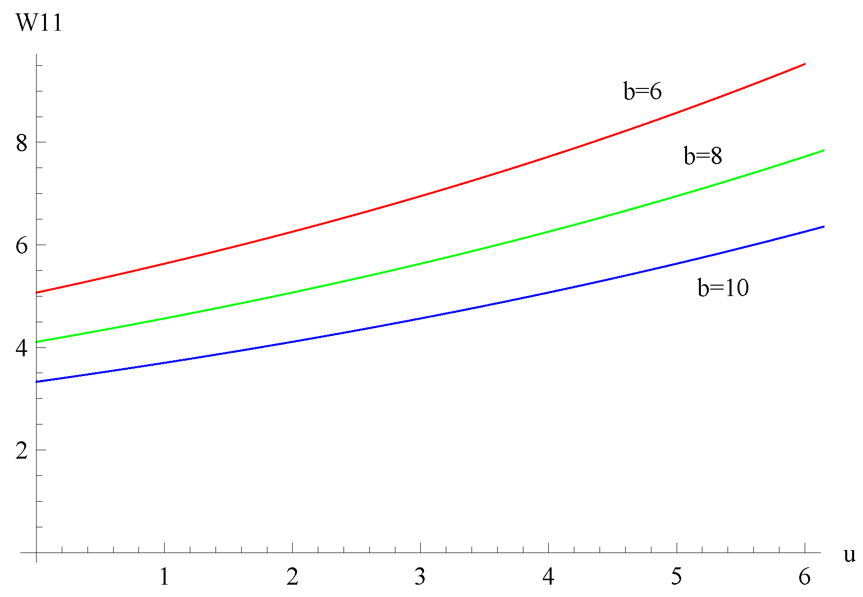
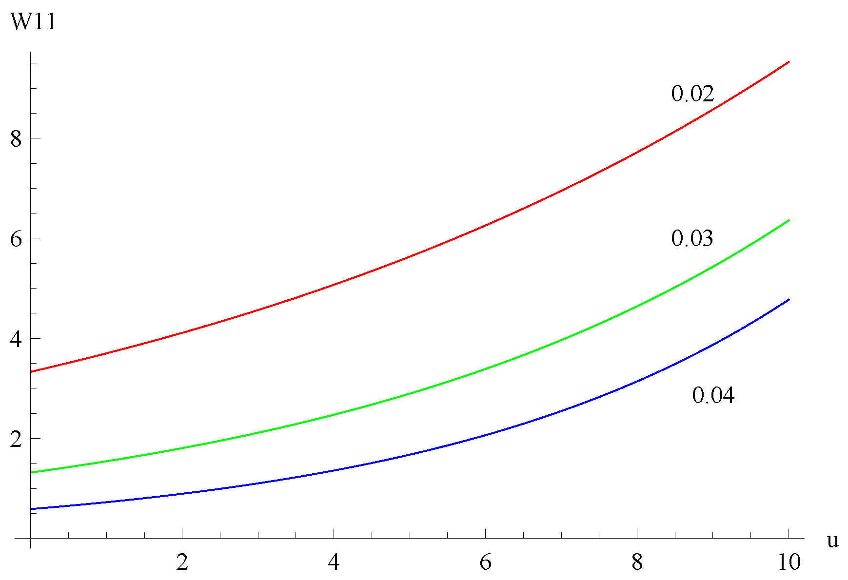
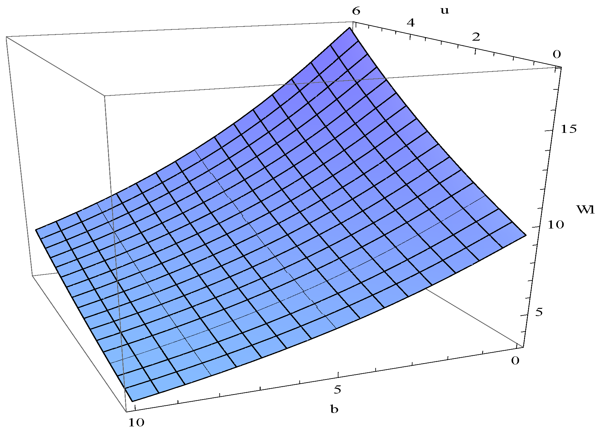
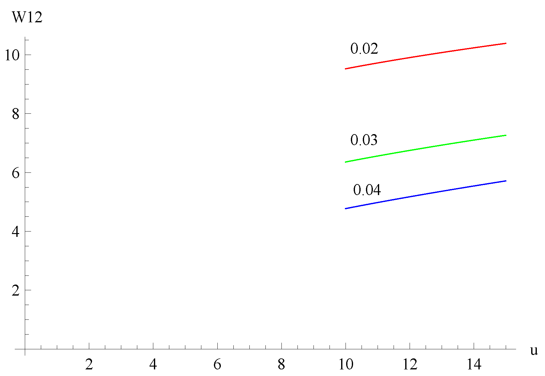
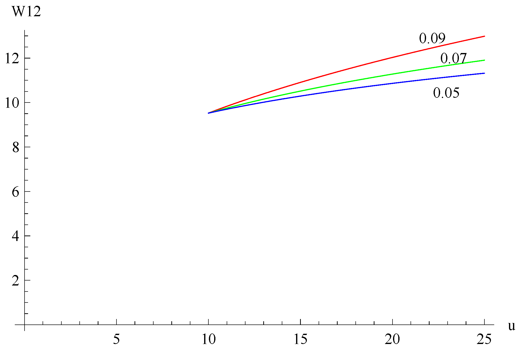
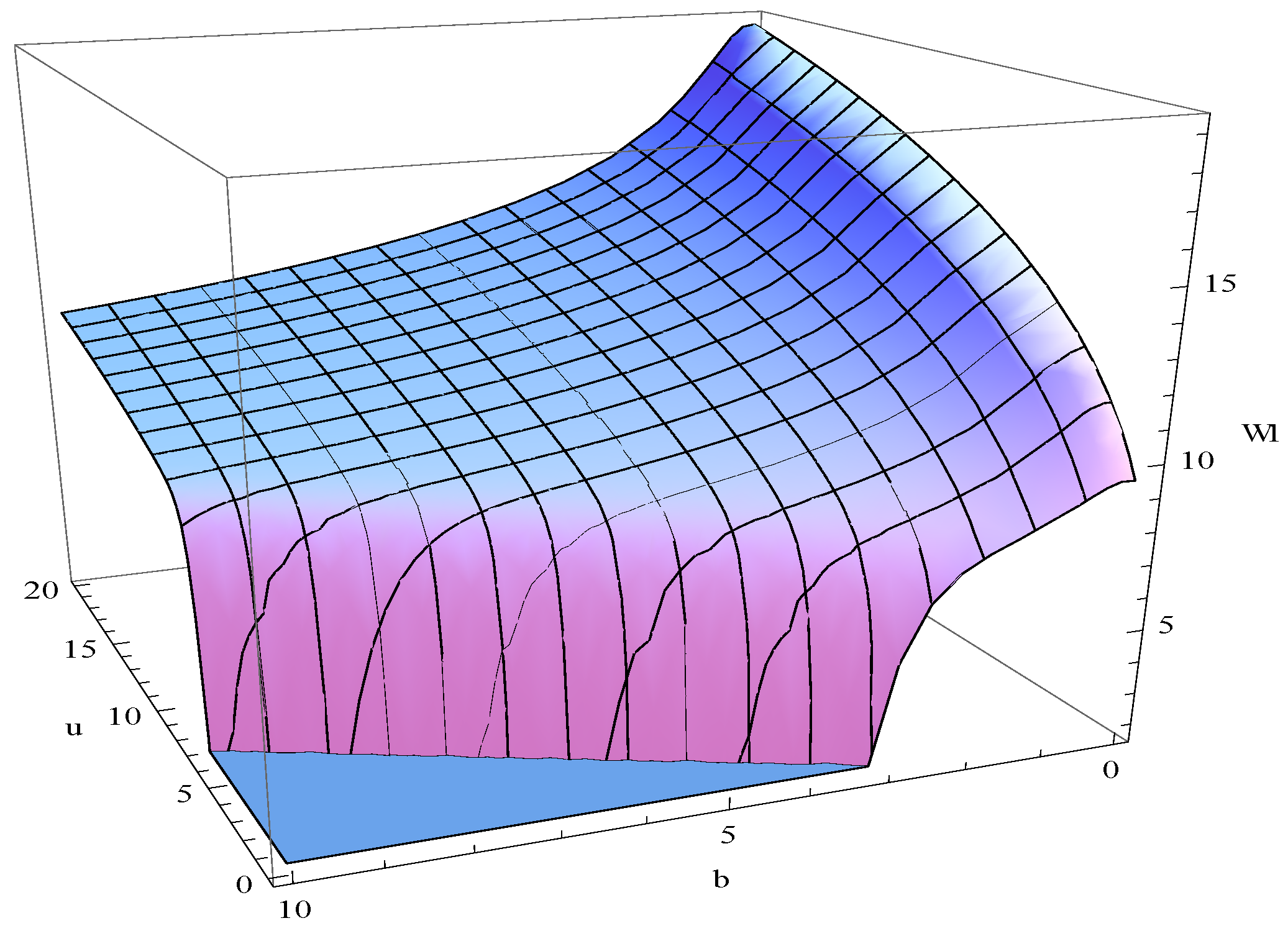
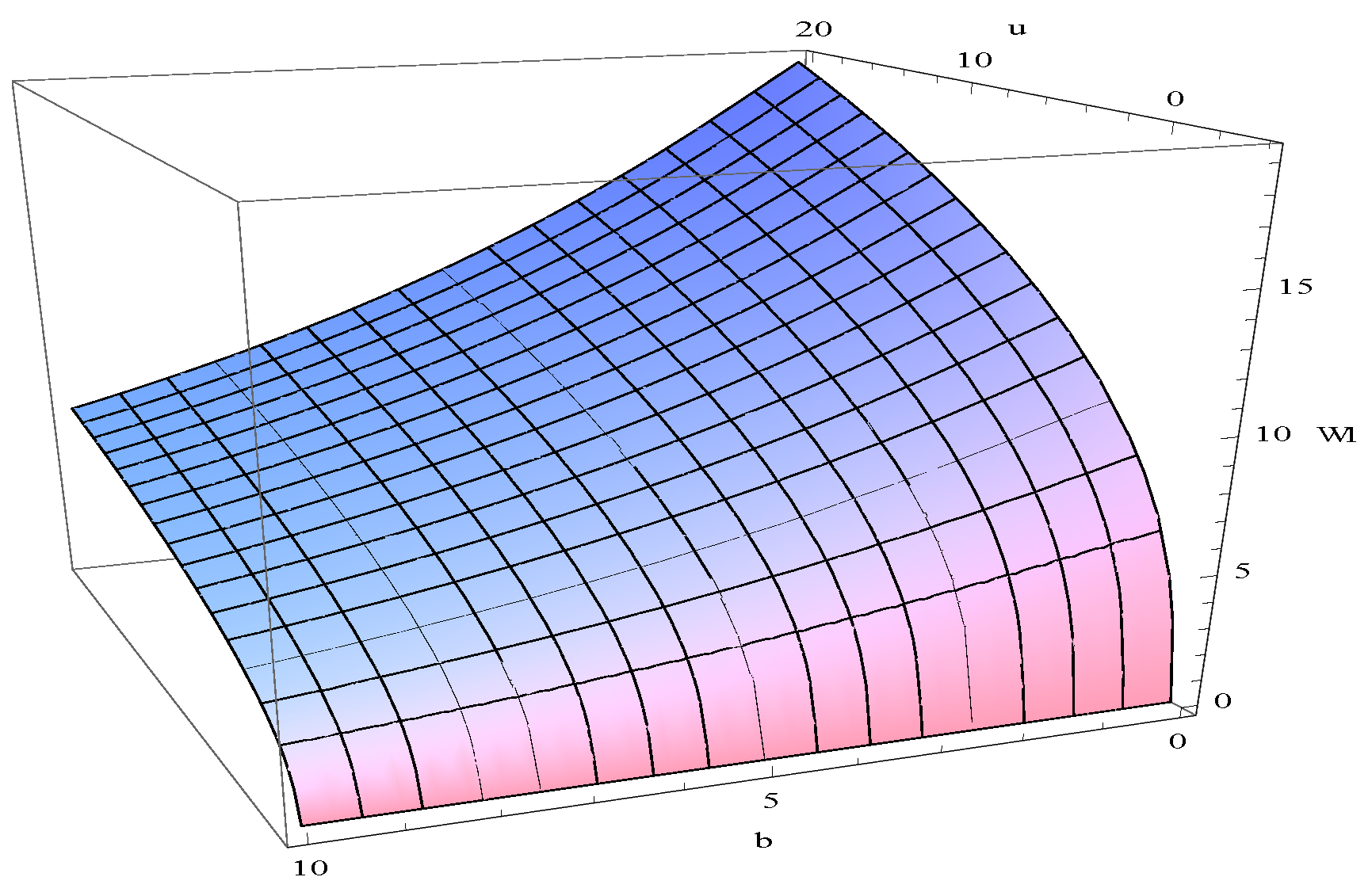
Suppose $\lambda =0.02$, $\mu =0.5$, $p_1=0.2$, $p_2=0.1$, $\gamma =0.08$, $\alpha =0.02$. Figure 1 shows the curves of $W_{11}(u,b)$ using the formulas derived above for dividend barriers of $b=6$, $b=8$ and $b=10$, respectively. Figure 2 shows the curves of $W_{11}(u,b)$ for $\alpha =0.02$, $\alpha =0.03$ and $\alpha =0.04(b=10)$, respectively. Figure 3 shows the surface of $W_{11}(u,b)$ with respect to two variables u and b. From the figures, we see that $W_{11}(u,b)$ decreases when b and α increase, respectively.

Example 2.

Suppose $\lambda =0.02$, $\beta =0.05$, $p_1=0.2$, $p_2=0.1$, and $\mu =0.5$. Figure 4 shows the curves of $W_{12}(u,b)$ for dividend barriers of $b=6$, $b=8$ and $b=10$. Figure 5 shows the curves of $W_{12}(u,b)$ for $\alpha =0.02$, $\alpha =0.03$ and $\alpha =0.04(b=10,\gamma =0.08)$. Figure 6 shows the curves of $W_{12}(u,b)$ for $\gamma =0.05$, $\gamma =0.07$ and $\gamma =0.09(b=10,\alpha =0.02)$. Figure 7 shows the surface of $W_{12}(u,b)$ with respect to variables u and b.

From Figure 4, Figure 5, Figure 6 and Figure 7, we can see that $W_{12}(u,b)$ is a decreasing function of b, $\alpha$, and $\gamma$, respectively. The results can be compared to the results of Peng et al. [5] who considered a compound Poisson risk model with a constant dividend barrier and liquid reserves in the case of absolute ruin. From the comparative results, we obtained the conclusion that the influence of parameter b on the moment of the present value of all dividends until absolute ruin is the same, regardless of whether a constant dividend barrier or the threshold dividend strategy is used. In addition, the effect of parameter $\gamma$ is the opposite. This is consistent with the actual situation.

Example 3.

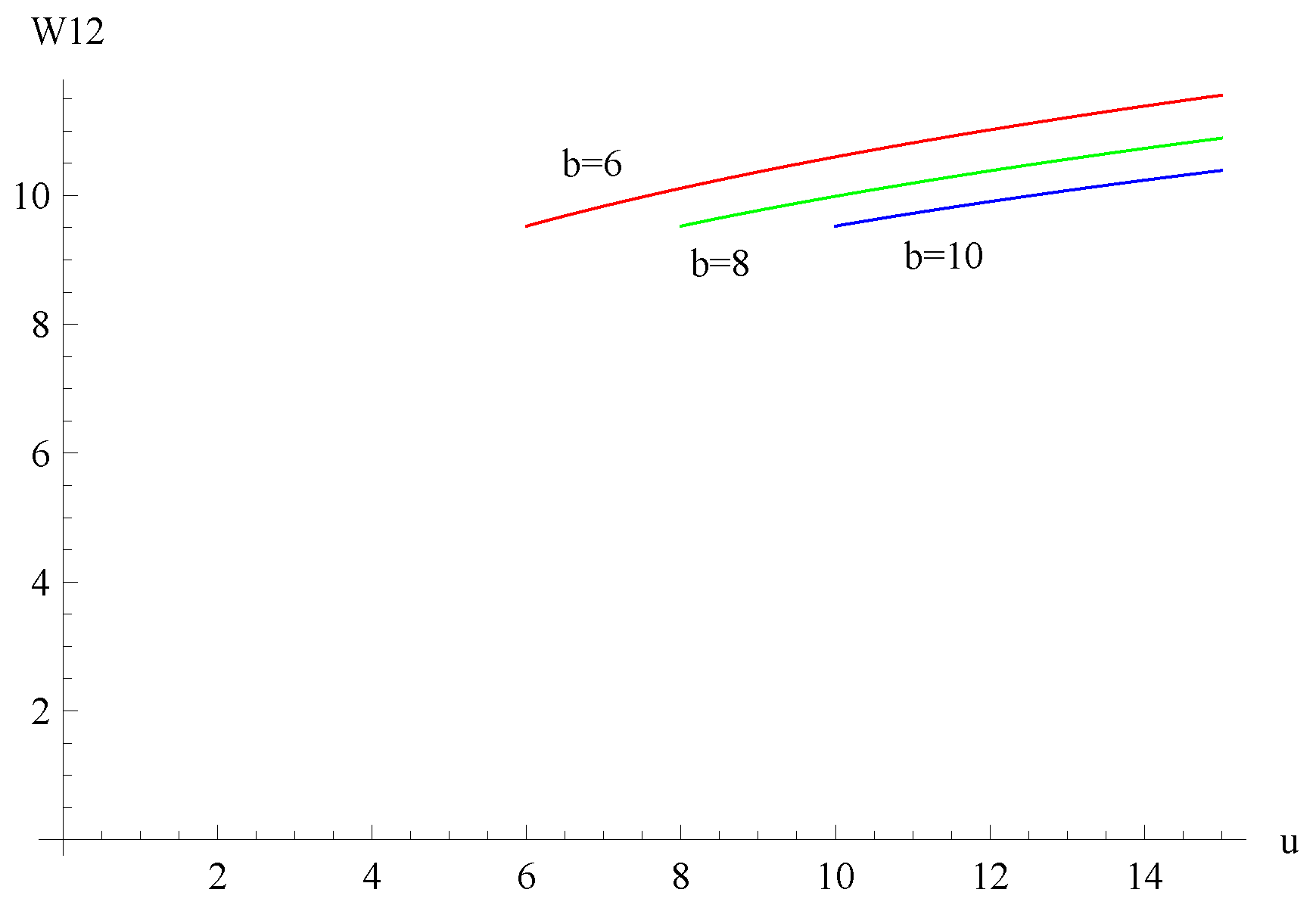
The parameters used were as follows: $\lambda =0.02$, $\beta =0.05$, $\alpha =0.02$, $\gamma =0.08$, $p_1=0.2$, $p_2=0.1$, $\mu =0.5$. Figure 8 shows the curves of $W_{13}(u,b)$ for dividend barriers of $b=6$, $b=8$ and $b=10$. Figure 9 shows the curves of $V_{13}(u,b)$ for $\alpha =0.01$, $\alpha =0.015$ and $\alpha =0.02(b=10,\gamma =0.08)$. Figure 10 shows the curves of $W_{13}(u,b)$ for $\beta =0.05$, $\beta =0.07$ and $\beta =0.09(b=10,\alpha =0.02)$. Figure 11 shows the surface of $W_{13}(u,b)$ with respect to variables u and b. The results show that $W_{13}(u,b)$ decreases as b, α, and β increase but increases as u increases.

4. The Gerber-Shiu Expected Discounted Penalty Function

Similarly, $\mathrm{\Phi }(u;b)$ can be expressed as

$$\begin{array}{c}\hfill \mathrm{\Phi }(u;b)=\left\{\begin{array}{c}{\mathrm{\Phi }}_2(u;b),u>b,\hfill \\ {\mathrm{\Phi }}_1(u;b),0\le u\le b,\hfill \\ {\mathrm{\Phi }}_3(u;b),-p_1/\beta <u<0.\hfill \end{array}\right.\end{array}$$

(57)

Similar to the arguments in Theorem 1, we can easily show that the Gerber-Shiu expected discounted penalty function satisfies the following integro-differential equations:

Theorem 4.

When $0\le u\le b$,

$$\begin{array}{cc}\hfill p_1{\mathrm{\Phi }}_1^{\prime }(u;b)=& (\lambda +\alpha ){\mathrm{\Phi }}_1(u;b)-\lambda \left[{\int }_0^u{\mathrm{\Phi }}_1(u-y;b)dG(y)\right.\hfill \\ & \left.+{\int }_u^{u+p_1/\beta }{\mathrm{\Phi }}_3(u-y;b)dG(y)+B(u)\right],\hfill \end{array}$$

(58)

and when $u>b$,

$$\begin{array}{cc}\hfill (\gamma u+p_2){\mathrm{\Phi }}_2^{\prime }(u;b)=& (\lambda +\alpha ){\mathrm{\Phi }}_2(u;b)-\lambda \left[{\int }_0^{u-b}{\mathrm{\Phi }}_2(u-y;b)dG(y)\right.\hfill \\ & \left.+{\int }_{u-b}^u{\mathrm{\Phi }}_1(u-y;b)dG(y)+{\int }_u^{u+p_1/\beta }{\mathrm{\Phi }}_3(u-y;b)dG(y)+B(u)\right],\hfill \end{array}$$

(59)

and when $-p_1/\beta <u<0$,

$$\begin{array}{cc}\hfill (\beta u+p_1){\mathrm{\Phi }}_3^{\prime }(u;b)=& (\lambda +\alpha ){\mathrm{\Phi }}_3(u;b)-\lambda {\int }_0^{u+p_1/\beta }{\mathrm{\Phi }}_3(u-y;b)dG(y)+B(u),\hfill \end{array}$$

(60)

with boundary conditions

$$\begin{array}{c}\hfill {\mathrm{\Phi }}_1(0+;b)={\mathrm{\Phi }}_3(0-;b),\end{array}$$

(61)

$$\begin{array}{c}\hfill {\mathrm{\Phi }}_1(b-;b)={\mathrm{\Phi }}_2(b+;b),\end{array}$$

(62)

$$\begin{array}{c}\hfill p_1{\mathrm{\Phi }}_1^{\prime }(b-;b)=(\gamma b+p_2){\mathrm{\Phi }}_2^{\prime }(b+;b),\end{array}$$

(63)

$$\begin{array}{c}\hfill {\mathrm{\Phi }}_1^{\prime }(0+;b)={\mathrm{\Phi }}_3^{\prime }(0-;b),\end{array}$$

(64)

where, ${\displaystyle B(u)={\int }_{u+p_1/\beta }^{\infty }\omega (u,y-u)dG(y)}$.

Theorem 5.

The integro-differential Equations (58)–(60) can be expressed by the Volterra equations

$$\begin{array}{c}\hfill {\mathrm{\Phi }}_1(u;b)={\int }_0^u{k}_1(u,x){\mathrm{\Phi }}_1(x;b)dx+{\psi }_1(u),0\le u\le b,\end{array}$$

(65)

$$\begin{array}{c}\hfill {\mathrm{\Phi }}_2(u;b)={\int }_b^u{k}_2(u,x){\mathrm{\Phi }}_2(x;b)dx+{\psi }_2(u),u>b,\end{array}$$

(66)

$$\begin{array}{c}\hfill {\mathrm{\Phi }}_3(u;b)={\int }_{-p_1/\beta }^u{k}_3(u,x){\mathrm{\Phi }}_3(x;b)dx+{\psi }_3(u),-p_1/\beta <u<0,\end{array}$$

(67)

where

$$\begin{array}{cc}\hfill k_1(u,x)=& \frac{\lambda +\alpha }{p_1}-\frac{\lambda }{p_1}G(u-x),\hfill \\ \hfill {\psi }_1(u)=& {\mathrm{\Phi }}_1(0;b)-\frac{\lambda }{p_1}{\int }_{-p_1/\beta }^0{\mathrm{\Phi }}_3(x;b)[G(u-x)-G(-x)]dx+\frac{\lambda }{p_1}{\int }_0^{u}B(x)dx,\hfill \\ \hfill k_2(u,x)=& \frac{\lambda +\alpha +\gamma }{\gamma u+p_2}-\frac{\lambda }{\gamma u+p_2}G(u-x),\hfill \\ \hfill {\psi }_2(u)=& \frac{\gamma b+p_2}{\gamma u+p_2}{\mathrm{\Phi }}_2(b;b)-\frac{\lambda }{\gamma u+p_2}{\int }_0^b{\mathrm{\Phi }}_1(x;b)[G(u-x)-G(b-x)]dx\hfill \\ & -\frac{\lambda }{\gamma u+p_2}{\int }_{-p_1/\beta }^0{\mathrm{\Phi }}_3(x;b))[G(u-x)-G(b-x)]dx\hfill \\ & -\frac{\lambda }{\gamma u+p_2}{\int }_0^{u}B(x)dx,\hfill \\ \hfill k_3(u,x)=& \frac{\lambda +\beta +\gamma }{\beta u+p_1}-\frac{\lambda }{\beta u+p_1}G(u-x),\hfill \\ \hfill {\psi }_3(u)=& \frac{\lambda }{\beta u+p_1}{\int }_0^{u}B(x)dx.\hfill \end{array}$$

Proof. 

In (58), integrating (58) over $(0,u)$ yields

$$\begin{array}{cc}\hfill p_1{\mathrm{\Phi }}_1(u;b)=& p_1{\mathrm{\Phi }}_1(0;b)+{\int }_0^u{\mathrm{\Phi }}_1(x;b)(\lambda +\alpha -\lambda G(u-x))dx\hfill \\ & -\lambda {\int }_{-p_1/\beta }^0[G(u-x)-G(-x)]dx-\lambda {\int }_0^{u}B(x)dx.\hfill \end{array}$$

(68)

In (68), integrating (68) over $(0,u)$, one concludes

$$\begin{array}{cc}\hfill p_1{\int }_0^u{\mathrm{\Phi }}_1(y;b)dy=& p_1{\mathrm{\Phi }}_1(0;b)u+{\int }_0^u\left[{\int }_0^y{\mathrm{\Phi }}_1(x;b)(\lambda +\alpha -\lambda G(y-x))dx\right]dy\hfill \\ & -\lambda {\int }_0^{u}G(y)dy,\hfill \end{array}$$

(69)

where, ${\displaystyle G(y)={\int }_{-p_1/\beta }^0{\mathrm{\Phi }}_3(x;b)(G(y-x)-G(-x))dx+{\int }_0^{y}B(x)dx}$, since

$$\begin{array}{c}\hfill {\int }_0^u\left[{\int }_0^y{\mathrm{\Phi }}_1(x;b)(\lambda +\alpha -\lambda G(y-x))dx\right]dy={\int }_0^u\left[{\int }_x^u{\mathrm{\Phi }}_1(x;b)(\lambda +\alpha -\lambda G(y-x))dy\right]dx.\end{array}$$

(70)

Substituting (70) into (69) yields (65).

Similarly to the proof of (65), we can obtain (66) and (67). ☐

Remark 1.

We point out that ${\psi }_1(u)$, ${\psi }_2(u)$, and ${\psi }_3(u)$ are absolutely integrable, and $k_1(u;b)$, $k_2(u;b)$, and $k_3(u;b)$ are all continuous. In accordance with Cai and Dickson [29], ${\mathrm{\Phi }}_1(u;b)$, ${\mathrm{\Phi }}_2(u;b)$ and ${\mathrm{\Phi }}_3(u;b)$ can be approximated recursively by Picards sequence, i.e.,

$$\begin{array}{c}\hfill {\mathrm{\Phi }}_1(u;b)={\psi }_1(u)+\sum _{n=1}^{\infty }{\int }_0^u{k}_{1n}(u,x){\psi }_1(x)dx,0\le u\le b,\end{array}$$

where, $k_{11}(u,x)=k_1(u,x)$, ${\displaystyle k_{1n}(u,x)={\int }_x^u{k}_1(u,y)k_{1,n-1}(y,x)dy,n=2,3,\dots }$.

$$\begin{array}{c}\hfill {\mathrm{\Phi }}_2(u;b)={\psi }_2(u)+\sum _{n=1}^{\infty }{\int }_b^u{k}_{2n}(u,x){\psi }_2(x)dx,u>b,\end{array}$$

where, $k_{21}(u,x)=k_2(u,x)$, ${\displaystyle k_{2n}(u,x)={\int }_x^u{k}_2(u,y)k_{2,n-1}(y,x)dy,n=2,3,\dots }$.

$$\begin{array}{c}\hfill {\mathrm{\Phi }}_3(u;b)={\psi }_3(u)+\sum _{n=1}^{\infty }{\int }_{-p_1/\beta }^u{k}_{3n}(u,x){\psi }_3(x)dx,0\le u\le b,\end{array}$$

where, $k_{31}(u,x)=k_3(u,x)$, ${\displaystyle k_{3n}(u,x)={\int }_x^u{k}_3(u,y)k_{3,n-1}(y,x)dy,n=2,3,\dots }$.

Hence, at least in theory, if we can provide these values of ${\mathrm{\Phi }}_1(0;b)$, ${\mathrm{\Phi }}_1^{\prime }(0;b)$, ${\mathrm{\Phi }}_2(b;b)$, ${\mathrm{\Phi }}_2^{\prime }(b;b)$, ${\mathrm{\Phi }}_3(-p_1/\beta ;b)$, and ${\mathrm{\Phi }}_3^{\prime }(-p_1/\beta ;b)$, we can obtain the exact expression of the solutions for ${\mathrm{\Phi }}_1(u;b)$, ${\mathrm{\Phi }}_2(u;b)$, and ${\mathrm{\Phi }}_3(u;b)$, recursively.

5. The Laplace Transform of Absolute Ruin Time

In this section, we set

$$\begin{array}{c}\hfill \phi (u;b)=\left\{\begin{array}{c}{\phi }_2(u;b),u>b,\hfill \\ {\phi }_1(u;b),0\le u\le b,\hfill \\ {\phi }_3(u;b),-p_1/\beta <u<0.\hfill \end{array}\right.\end{array}$$

(71)

Theorem 6.

When $0\le u\le b$,

$$\begin{array}{cc}\hfill p_1{\phi }_1^{\prime }(u;b)=& (\lambda +\rho ){\phi }_1(u;b)-\lambda \left[{\int }_0^u{\phi }_1(u-y;b)dG(y)\right.\hfill \\ & \left.+{\int }_u^{u+p_1/\beta }{\phi }_3(u-y;b)dG(y)+\overline{G}(u+\frac{p_1}{\beta })\right],\hfill \end{array}$$

(72)

and when $u>b$,

$$\begin{array}{cc}\hfill (\gamma u+p_2){\phi }_2^{\prime }(u;b)& =(\lambda +\rho ){\phi }_2(u;b)-\lambda \left[{\int }_0^{u-b}{\phi }_2(u-y;b)dG(y)\right.\hfill \\ & +{\int }_{u-b}^u{\phi }_1(u-y;b)dG(y)+{\int }_u^{u+p_1/\beta }{\phi }_3(u-y;b)dG(y)\hfill \\ & \left.+\overline{G}(u+\frac{p_1}{\beta })\right],\hfill \end{array}$$

(73)

and when $-p_1/\beta <u<0$,

$$\begin{array}{cc}\hfill (\beta u+p_1){\phi }_3^{\prime }(u;b)=& (\lambda +\rho ){\phi }_3(u;b)-\lambda \left[{\int }_0^{u+p_1/\beta }{\phi }_3(u-y;b)dG(y)\right.\hfill \\ & \left.+\overline{G}(u+\frac{p_1}{\beta })\right],\hfill \end{array}$$

(74)

with the conditions

$$\begin{array}{c}\hfill {\phi }_1(0+;b)={\phi }_3(0-;b),\end{array}$$

(75)

$$\begin{array}{c}\hfill {\phi }_1(b-;b)={\phi }_2(b+;b),\end{array}$$

(76)

$$\begin{array}{c}\hfill {\phi }_1^{\prime }(0+;b)={\phi }_3^{\prime }(0-;b),\end{array}$$

(77)

$$\begin{array}{c}\hfill p_1{\phi }_1^{\prime }(b-;b)=(\gamma b+p_2){\phi }_2^{\prime }(b+;b),\end{array}$$

(78)

$$\begin{array}{c}\hfill \underset{u\to -p_1/\beta }{\lim }{\phi }_3(-\frac{p_1}{\beta };b)=\frac{\lambda }{\lambda +\rho },\end{array}$$

(79)

$$\begin{array}{c}\hfill \underset{u\to \infty }{\lim }{\phi }_2(-\frac{p_1}{\beta };b)=0,\end{array}$$

(80)

where, Equation (80) is acquired from the fact that $T_b=\infty$ and $E[e^{-\rho T_b}I(T_b<\infty )|R_0^{u,b}=u]=0$ when $u\to \infty$.

In the following, we solve the closed form expression for $\phi (u;b)$ according to the exponential distribution of claims with mean $\mu$. By applying the operator $\left({\displaystyle \frac{d}{du}+\frac{1}{\mu }}\right)$ on (72)–(74), respectively, and then rearranging them, one deduces

$$\begin{array}{c}\hfill {\phi }_1^{″}(u;b)+\left(\frac{1}{\mu }-\frac{\lambda +\rho }{p_1}\right){\phi }_1^{\prime }(u;b)-\frac{\rho }{\mu p_1}{\phi }_1(u;b)=0,0\le u\le b,\end{array}$$

(81)

$$\begin{array}{c}\hfill (\gamma u+p_2){\phi }_2^{″}(u;b)+\left(\frac{\gamma u+p_2}{\mu }+\gamma -\lambda -\rho \right){\phi }_2^{\prime }(u;b)-\frac{\rho }{\mu }{\phi }_1(u;b)=0,u>b,\end{array}$$

(82)

$$\begin{array}{c}\hfill (\beta u+p_1){\phi }_3^{″}(u;b)+\left(\frac{\beta u+p_1}{\mu }+\beta -\lambda -\rho \right){\phi }_3^{\prime }(u;b)-\frac{\rho }{\mu }{\phi }_3(u;b)=0,-p_1/\beta <u\le 0.\end{array}$$

(83)

By comparing (81)–(83) with (36)–(38) respectively, we have

$$\begin{array}{c}\hfill {\phi }_1(u;b)=m_1{e}^{{\sigma }_{1}u}+m_2{e}^{{\sigma }_{2}u},-p_1/\beta <u\le 0,\end{array}$$

(84)

where, $m_1$ and $m_2$ are arbitrary constants, ${\displaystyle q_1=\frac{1}{\mu }-\frac{\lambda +\rho }{p_1}}$ and ${\displaystyle q_2=-\frac{\rho }{\mu p_1}}$ satisfying $q_1^2-4q_2>0$, i.e.,

$$\begin{array}{c}\hfill {\sigma }_1=\frac{-q_1+\sqrt{q_1^2-4q_2}}{2},{\sigma }_2=\frac{-q_1-\sqrt{q_1^2-4q_2}}{2},\end{array}$$

(85)

and

$$\begin{array}{c}\hfill {\phi }_2(u;b)=m_3{\tau }_3(u)+m_4{\tau }_4(u),u>b,\end{array}$$

(86)

$$\begin{array}{c}\hfill {\phi }_3(u;b)=m_5{\tau }_5(u)+m_6{\tau }_6(u),-p_1/\beta <u\le 0,\end{array}$$

(87)

with

$$\begin{array}{cc}\hfill {\tau }_3(u)& =\exp \{-\frac{\gamma u+p_2}{\gamma \mu }\}·U\left(1-\frac{\lambda }{\gamma },1-\frac{\lambda +\rho }{\gamma };\frac{\gamma u+p_2}{\gamma \mu }\right),\hfill \\ \hfill {\tau }_4(u)& ={\left(\frac{\gamma u+p_2}{\gamma \mu }\right)}^{(\lambda +\rho )/\gamma }·\exp \{-\frac{\gamma u+p_2}{\gamma \mu }\}·M\left(1+\frac{\rho }{\gamma },1+\frac{\lambda +\rho }{\gamma };\frac{\gamma u+p_2}{\gamma \mu }\right),\hfill \\ \hfill {\tau }_5(u)& =\exp \{-\frac{\beta u+p_1}{\beta \mu }\}·U\left(1-\frac{\lambda }{\beta },1-\frac{\lambda +\rho }{\beta };\frac{\beta u+p_1}{\beta \mu }\right),\hfill \\ \hfill {\tau }_6(u)& ={\left(\frac{\beta u+p_1}{\beta \mu }\right)}^{(\lambda +\rho )/\beta }·\exp \{-\frac{\beta u+p_1}{\beta \mu }\}·M\left(1+\frac{\rho }{\beta },1+\frac{\lambda +\rho }{\beta };\frac{\beta u+p_1}{\beta \mu }\right).\hfill \end{array}$$

If $\beta \ne \lambda +\rho$, we have

$$\begin{array}{c}\hfill {\displaystyle \underset{u\downarrow -p_1/\beta }{\lim }{\tau }_5(u)=\frac{\Gamma \left({\displaystyle \frac{\lambda +\rho }{\beta }}\right)}{\Gamma \left({\displaystyle \frac{\beta +\rho }{\beta }}\right)}={\tau }_5(-p_1/\beta ),\underset{u\downarrow -p_1/\beta }{\lim }{\tau }_6(u)=0.}\end{array}$$

(88)

From (75)–(80), (84), (86)–(88), it follows that

$$\begin{array}{c}\hfill \left\{\begin{array}{c}{m}_1+m_2-m_5{\tau }_5(0)-m_6{\tau }_6(0)=0,\hfill \\ m_1{e}^{{\sigma }_{1}b}+m_2{e}^{{\sigma }_{2}b}-m_3{\tau }_3(b)-m_4{\tau }_4(b)=0,\hfill \\ m_1{\sigma }_1+m_2{\sigma }_2-m_5{\tau }_5^{\prime }(0)-m_6{\tau }_6^{\prime }(0)=0,\hfill \\ m_1{p}_1{\sigma }_1{e}^{{\sigma }_{1}b}+m_2{p}_1{\sigma }_2{e}^{{\sigma }_{2}b}-m_3(\gamma b+p_2){\tau }_3^{\prime }(b)-m_4(\gamma b+p_2){\tau }_4^{\prime }(b)=0,\hfill \\ {\displaystyle m_5{\tau }_5(-p_1/\beta )=\frac{\lambda }{\lambda +\rho },}\hfill \\ m_3{\tau }_3(\infty )+m_4{\tau }_4(\infty )=0.\hfill \end{array}\right.\end{array}$$

(89)

We let $\mathrm{\Pi }$ be the the matrix, defined as

$$\mathrm{\Pi }=\left(\begin{array}{cccccc}1& 1& 0& 0& -{\tau }_5(0)& -{\tau }_6(0)\\ e^{{\sigma }_{1}b}& e^{{\sigma }_{2}b}& -{\tau }_3(0)& -{\tau }_4(0)& 0& 0\\ {\sigma }_1& {\sigma }_1& 0& 0& -{\tau }_5^{\prime }(0)& -{\tau }_6^{\prime }(0)\\ p_1{\sigma }_1{e}^{{\sigma }_{1}b}& p_1{\sigma }_2{e}^{{\sigma }_{2}b}& -(\gamma b+p_2){\tau }_3^{\prime }(b)& -(\gamma b+p_2){\tau }_4^{\prime }(b)& 0& 0\\ 0& 0& 0& 0& {\tau }_5(-p_1/\beta )& 0\\ 0& 0& {\tau }_3(\infty )& {\tau }_4(\infty )& 0& 0\end{array}\right),$$

and the column vector $\overrightarrow{B}$ is defined as

$$\overrightarrow{B}={(0,0,0,0,\frac{\lambda }{\lambda +\rho },0)}^T,$$

where, T denotes the transpose. Let ${\mathrm{\Pi }}_{\mathbf{i}}$ denote the matrix except that the ith column of $\mathrm{\Pi }$ is replaced by $\overrightarrow{B}$. Then, we have

$$m_i=\frac{det({\mathrm{\Pi }}_{\mathbf{i}})}{det(\mathrm{\Pi })},i=1,2,3,4,5,6,$$

where, $det(·)$ denotes the determinant of a matrix. Hence, we have provided the closed form expressions for ${\phi }_i(u;b),i=1,2,3$.

6. The Time to Reach the Dividend Barrier

Let us explore how long it takes for the risk reserve process to attain the barrier b from the initial reserve u without absolute ruin. Let ${\chi }_b$ denote the first time that the risk reserve arrives at b, define

$$\mathrm{\Psi }(u;b)=E[e^{-\rho {\chi }_b}I({\chi }_b<T)|R_0^{u,b}=u],\rho >0.$$

(90)

For notational convenience, we set

$$\begin{array}{c}\hfill \mathrm{\Psi }(u;b)=\left\{\begin{array}{c}{\mathrm{\Psi }}_1(u;b),0\le u\le b,\hfill \\ {\mathrm{\Psi }}_2(u;b),-p_1/\beta <u<0.\hfill \end{array}\right.\end{array}$$

(91)

Using a method similar to Theorem 1, we have

For $0\le u\le b$,

$$\begin{array}{cc}\hfill p_1{\mathrm{\Psi }}_1^{\prime }(u;b)=& (\lambda +\rho ){\mathrm{\Psi }}_1(u;b)-\lambda \left[{\int }_0^u{\mathrm{\Psi }}_1(u-y;b)dG(y)\right.\hfill \\ & \left.+{\int }_u^{u+p_1/\beta }{\mathrm{\Psi }}_2(u-y;b)dG(y)\right],\hfill \end{array}$$

(92)

and, for $-p_1/\beta <u<0$,

$$\begin{array}{c}\hfill (\beta u+p_1){\mathrm{\Psi }}_2^{\prime }(u;b)=(\lambda +\rho ){\mathrm{\Psi }}_2(u;b)-\lambda [{\int }_0^{u+p_1/\beta }{\mathrm{\Psi }}_2(u-y;b)dG(y)],\end{array}$$

(93)

with boundary conditions

$$\begin{array}{c}{\mathrm{\Psi }}_1(0+;b)={\mathrm{\Psi }}_2(0-;b),\hfill \\ {\mathrm{\Psi }}_1^{{}^{\prime }}(0+;b)={\mathrm{\Psi }}_2^{{}^{\prime }}(0-;b)\hfill \\ \underset{u\to -p_1/\beta }{\lim }{\mathrm{\Psi }}_2(u;b)=0,\hfill \\ {\mathrm{\Psi }}_1(b;b)=1.\hfill \end{array}$$

Using the same methods as in Section 5, we can get the explicit expressions for ${\mathrm{\Psi }}_1(u;b)$ and ${\mathrm{\Psi }}_2(u;b)$ when the claim size is exponentially distributed with mean $\mu$. We omit it.

References

- Cai, J. On the time value of absolute ruin with debit interest. Adv. Appl. Probab. 2007, 39, 343–359. [Google Scholar] [CrossRef]
- Wang, C.W.; Yin, C.C. Dividend payments in the classical risk model under absolute ruin with debit interest. Appl. Stoch. Model. Bus. 2009, 25, 247–262. [Google Scholar] [CrossRef]
- Wang, C.W.; Yin, C.C.; Li, E.Q. On the classical risk model with credit and debit interests under absolute ruin. Stat. Probab. Lett. 2010, 80, 427–436. [Google Scholar] [CrossRef]
- Yuan, H.L.; Hu, Y.J.; Qin, Q.Q. Absolute ruin problems for the risk process with interest and a constant dividend barrier. Wuhan Univ. J. Nat. Sci. 2011, 16, 199–205. [Google Scholar] [CrossRef]
- Peng, D.; Liu, D.H.; Hou, Z.T. Absolute ruin problems in a compound Poisson risk model with constant dividend barrier and liquid reserves. Adv. Differ. Equ. 2016, 2016. [Google Scholar] [CrossRef]
- Wang, C.W.; Du, X.G.; Chen, Q.Y. On the compound Poisson risk model with debit interest and a threshold dividend strategy. In Proceedings of the Information Computing and Applications: Second International Conference ICICA, Qinhuangdao, China, 28–31 October 2011; Volume 243, pp. 596–603. [Google Scholar]
- Li, S.M.; Lu, Y. Moments of the dividend payments and related problems in a Markov-modulated risk model. N. Am. Actuar. J. 2007, 11, 65–76. [Google Scholar] [CrossRef]
- Huu, N.V.; Hoang, V.Q.; Ngoc, T.M. Central limit theorem for functional of jump Markov processes. Vietnam J. Math. 2005, 33, 443–461. [Google Scholar]
- Luo, S.Z.; Taksar, M. On absolute ruin minimization under a diffusion approximation model. Insur. Math. Econ. 2011, 48, 123–133. [Google Scholar] [CrossRef]
- Yang, Y.; Liu, J.; Gao, Q. Asymptotics for the infinite-time absolute ruin probabilities in time-dependent renewal risk models. Sci. Sin. Math. 2013, 43, 173–184. [Google Scholar] [CrossRef]
- Yang, Y.; Wang, K.Y.; Liu, J. Asymptotics and uniform asymptotics for finite-time and infinite-time absolute ruin probabilities in a dependent compound renewal risk model. J. Math. Anal. Appl. 2013, 398, 352–361. [Google Scholar] [CrossRef]
- Yu, W.G. Some results on absolute ruin in the perturbed insurance risk model with investment and debit interests. Econ. Model. 2013, 31, 625–634. [Google Scholar] [CrossRef]
- Cai, J.; Yang, H.L. On the decomposition of the absolute ruin probability in a perturbed compound Poisson surplus process with debit interest. Ann. Oper. Res. 2014, 212, 61–77. [Google Scholar] [CrossRef]
- Zhu, J.X. Optimal dividend control for a generalized risk model with investment incomes and debit interest. Scand. Actua. J. 2013, 2013, 140–162. [Google Scholar] [CrossRef] [Green Version]
- Zhu, J.X. Singular optimal dividend control for the regime-switching Cramér-Lundberg model with credit and debit interest. J. Comput. Appl. Math. 2014, 257, 212–239. [Google Scholar] [CrossRef]
- Bi, X.C.; Zhang, S.G. Minimizing the risk of absolute ruin under a diffusion approximation model with reinsurance and investment. J. Syst. Sci. Complex. 2015, 28, 144–155. [Google Scholar] [CrossRef]
- Liu, J.J.; Yang, Y. Infinite-time absolute ruin in dependent renewal risk models with constant force of interest. Stoch. Models. 2017, 33, 97–115. [Google Scholar] [CrossRef]
- Zeng, Y.; Li, Z. Optimal time-consistent investment and reinsurance policies for mean-variance insurers. Insur. Math. Econ. 2011, 49, 145–154. [Google Scholar] [CrossRef]
- Zeng, Y.; Li, D.; Chen, Z.; Yang, Z. Ambiguity aversion and optimal derivative-based pension investment with stochastic income and volatility. J. Econ. Dyn. Control. 2018, 88, 70–103. [Google Scholar] [CrossRef]
- Peng, J.Y.; Wang, D.C. Asymptotics for ruin probabilities of a non-standard renewal risk model with dependence structures and exponential Lévy process investment returns. J. Ind. Manag. Optim. 2017, 13, 155–185. [Google Scholar]
- Peng, J.Y.; Wang, D.C. Uniform asymptotics for ruin probabilities in a dependent renewal risk model with stochastic return on investments. Stochastics. 2018, 90, 432–471. [Google Scholar] [CrossRef]
- Avram, F.; Perez, J.; Yamazaki, K. Spectrally negative Lévy processes with Parisian reflection below and classical reflection above. Stoch. Proc. Appl. 2018, 128, 255–290. [Google Scholar] [CrossRef] [Green Version]
- Albrecher, H.; Claramunt, M.; Marmol, M. On the distribution of dividend payments in a Sparre Andersen model with generalized Erlang(n) interclaim times. Insur. Math. Econ. 2005, 37, 324–334. [Google Scholar] [CrossRef]
- Wan, N. Dividend payments with a threshold strategy in the compound Poisson risk model perturbed by diffusion. Insur. Math. Econ. 2007, 40, 509–532. [Google Scholar] [CrossRef]
- Paulsen, J.; Gjessing, H.K. Ruin theory with stochastic economic environment. Adv. Appl. Probab. 1997, 29, 965–985. [Google Scholar] [CrossRef]
- Cai, J.; Yang, H.L. Ruin in the perturbed compound Poisson risk process under interest force. Adv. Appl. Probab. 2005, 37, 819–835. [Google Scholar] [CrossRef] [Green Version]
- Salter, L.J. Confluent Hypergeometric Functions; Cambridge University Press: London, UK, 1960. [Google Scholar]
- Seaborn, J.B. Hypergeometric Functions and Their Applications; Springer: New York, NY, USA, 1991. [Google Scholar]
- Cai, J.; Dickson, D.C.M. On the expected discounted penalty function at ruin of a surplus process with interest. Insur. Math. Econ. 2002, 30, 389–404. [Google Scholar] [CrossRef]
Figure 1.
The curves of for dividend barriers of , and .
Figure 2.
The curves of for , and .
Figure 3.
The surface of with respect to two variables u and b.
Figure 4.
Figure 5.
Figure 6.
Figure 7.
The surface of with respect to variables u and b.
Figure 8.
Figure 9.
Figure 10.
Figure 11.
© 2018 by the authors. Licensee MDPI, Basel, Switzerland. This article is an open access article distributed under the terms and conditions of the Creative Commons Attribution (CC BY) license (http://creativecommons.org/licenses/by/4.0/).
Share and Cite
MDPI and ACS Style
Yu, W.; Huang, Y.; Cui, C. The Absolute Ruin Insurance Risk Model with a Threshold Dividend Strategy. Symmetry 2018, 10, 377. https://doi.org/10.3390/sym10090377
AMA Style
Yu W, Huang Y, Cui C. The Absolute Ruin Insurance Risk Model with a Threshold Dividend Strategy. Symmetry. 2018; 10(9):377. https://doi.org/10.3390/sym10090377
Chicago/Turabian StyleYu, Wenguang, Yujuan Huang, and Chaoran Cui. 2018. "The Absolute Ruin Insurance Risk Model with a Threshold Dividend Strategy" Symmetry 10, no. 9: 377. https://doi.org/10.3390/sym10090377
Note that from the first issue of 2016, this journal uses article numbers instead of page numbers. See further details here.