Decaying Dark Energy in Light of the Latest Cosmological Dataset


Department of Theoretical Physics and History of Science, University of the Basque Country UPV/EHU, Faculty of Science and Technology, Barrio Sarriena s/n, 48940 Leioa, Spain
Symmetry 2018, 10(9), 372; https://doi.org/10.3390/sym10090372
Submission received: 2 August 2018
/
Revised: 13 August 2018
/
Accepted: 21 August 2018
/
Published: 1 September 2018
(This article belongs to the Special Issue Cosmological Inflation, Dark Matter and Dark Energy)
Abstract
:Decaying Dark Energy models modify the background evolution of the most common observables, such as the Hubble function, the luminosity distance and the Cosmic Microwave Background temperature–redshift scaling relation. We use the most recent observationally-determined datasets, including Supernovae Type Ia and Gamma Ray Bursts data, along with and Cosmic Microwave Background temperature versus z data and the reduced Cosmic Microwave Background parameters, to improve the previous constraints on these models. We perform a Monte Carlo Markov Chain analysis to constrain the parameter space, on the basis of two distinct methods. In view of the first method, the Hubble constant and the matter density are left to vary freely. In this case, our results are compatible with previous analyses associated with decaying Dark Energy models, as well as with the most recent description of the cosmological background. In view of the second method, we set the Hubble constant and the matter density to their best fit values obtained by the Planck satellite, reducing the parameter space to two dimensions, and improving the existent constraints on the model’s parameters. Our results suggest that the accelerated expansion of the Universe is well described by the cosmological constant, and we argue that forthcoming observations will play a determinant role to constrain/rule out decaying Dark Energy.
1. Introduction
In the last decades, several observations have pointed out that the Universe is in an ongoing period of accelerated expansion that is driven by the presence of an exotic fluid with negative pressure [1,2,3,4,5,6,7,8,9,10,11,12]. Its simplest form is a cosmological constant , having an equation of state . More complicated prescriptions lead to the so-called Dark Energy (DE). Although several models have been proposed to explain DE [13,14,15,16,17,18,19,20,21,22,23,24,25,26,27], the observations have only determined that it accounts for of the total energy-density budget of the Universe, while its fundamental nature is still unknown (see, for instance, the reviews [28,29]). In addition, we should mention that the accelerated expansion of the Universe could be explained by several modifications of the gravitational action. For example, introducing higher order terms of the Ricci curvature in the Hilbert–Einstein Lagrangian, gives rise to an effective matter stress–energy tensor which could drive the current accelerated expansion (see, for example, the reviews [12,30,31,32,33,34,35]). Another alternative for reproducing the dark energy effects is by introducing non-derivative terms interactions in the action, in addition to the Einstein–Hilbert action term, such that it creates the effect of a massive graviton [36,37,38].
We are interested in exploring a specific decaying DE model, , leading to creation/annihilation of photons and Dark Matter (DM) particles. The model is based on the theoretical framework developed in [39,40,41,42,43], while the thermodynamic features have been developed in [44,45]. Since DE continuously decays into photons and/or DM particles along the cosmic evolution, the relation between the temperature of the Cosmic Microwave Background (CMB) radiation and the redshift is modified.
In the framework of the standard cosmological model, the Universe expands adiabatically and, as consequence of the entropy and photon number conservation, the temperature of the CMB radiation scales linearly with redshift, . Nevertheless, in those models where conservation laws are violated, the creation or annihilation of photons can lead to distortions in the blackbody spectrum of the CMB and, consequently, to deviations of the standard CMB temperature–redshift scaling relation. Such deviations are usually explored with a phenomenological parameterization, such as proposed in [41], where is a constant parameter ( means adiabatic evolution), and is the CMB temperature at , which has been strongly constrained with COBE-FIRAS experiment, K [46]. The parameter has been constrained using two methodologies: (a) the fine structure lines corresponding to the transition energies of atoms or molecules, present in quasar spectra, and excited by the CMB photon [47]; and (b) the multi-frequency measurements of the Sunyaev-Zel’dovich (SZ) effect [48,49,50]. Recent results based on data released by the Planck satellite and the South Pole Telescope (SPT) have led to sub-percent constraints on which results to be compatible with zero at level (more details can be found in [11,51,52,53,54,55,56]).
In this paper, we start with the theoretical results obtained in [44,45]. Such a model has been constrained using luminosity distance measurements from Supernovae Type Ia (SNIa), differential age data, Baryonic Acoustic Oscillation (BAO), the CMB temperature–redshift relation, and the CMB shift parameter. Since the latter depends on the redshift of the last surface scattering, , it represents a very high redshift probe. On the contrary, other datasets were used to probe the Universe at low redshift, . We aim to improve those constraints performing two different analysis: first, we constrain the whole parameter space to study the possibility of the model to alleviate the tension in the Hubble constant (see Section 5.4 in [10] for the latest results on the subject); and, second, we adopt the Planck cosmology to improve the constraint on the remaining parameters. Thus, we retain the SNIa, and use the most recent measurements the differential age, BAO, and the CMB temperature–redshift data. In addition, we use luminosity distances data of Gamma Ray Burst (GRB), which allow us to extend the redshift range till . Finally, we also use the reduced (compressed) set of parameters from CMB constraints [10].
The paper is organized as follows. In Section 2, we summarize the theoretical framework starting from the general Friedman–Robertson–Walker (FRW) metric, and point out the modification to the cosmological background arising from the violation of the conservation laws. In Section 3, we present the datasets used in the analysis, and the methodology implemented to explore the parameter space. The results are shown and discussed in Section 4 and, finally, in Section 5, we give our conclusions.
2. Theoretical Framework
The starting point is the well-known FRW metric
where is the scale factor and k is the curvature of the space time [57]. In General Relativity (GR), one obtains the following Friedman equations:
where the total pressure is , the total density is , and and are the density and pressure of DE, respectively. Following [44,45], we set both the “bare” cosmological constant and the curvature k equal to 0.
In the standard cosmology, the Bianchi identities hold and the stress–energy momentum is locally conserved
Adopting a perfect fluid, the previous relation can recast as
where is the definition of the Hubble parameter. Thus, each component is conserved. Nevertheless, due to the photon/matter creation/annihilation happening in the case of decaying DE, the conservation equation is recast in the following relations:
where is a free parameter determining the equation of state of radiation and, and account for the decay of DE. describe the physical mechanism leading to the production of particles (see, for instance, the thermogravitational quantum creation theory [40] or the quintessence scalar field cosmology [14]), and must be small enough in order to have the current density of radiation matching the observational constraints. Assuming , and defining
the parameter can be obtained from the Equation (8)
Following [44,45], one can adopt a power law model
then, writing Equation (2) at the present epoch, one can obtain , where is the matter density fraction at . It is very straightforward to verify that setting the power law index leads to the cosmological constant. From Equation (8), it is also possible to write down an effective equation of state for the DE [45]:
Let us note that the standard Hubble parameter is recovered by setting in Equation (13). Having the Hubble parameter allows us to compute the luminosity distance as follows
where we have defined .
Finally, following the approach originally proposed in [39], combining the Equations (6)–(8), with the equation for the number density conservation
where is the photon source, and the Gibbs Law
one obtains, through the use of thermodynamic identities, the following CMB temperature redshift relation (see for more details [43,45]):
Again, setting gives the standard relation . Equations (13), (14) and (17) can be easily implemented to test the decaying DE scenario. To show the effectiveness of these observables in constraining the cosmological model, we depict in Figure 1 their scalings as a function of the redshift for different value of the parameters and m, while we set and to their best fit from Planck satellite. In Figure 1a–c, we fix (which represents its standard value) while varying m in the range to show its impact on the Hubble constant, the luminosity distance and the CMB temperature. On the contrary, in Figure 1d, we set (standard value) and vary illustrating how much the -redshift relation is affected. The redshift ranges in the panels are set to the ones of the datasets. Looking at the plots, it is clear that the data will be really sensible to a variation of , while m will be more difficult to constrain.
3. Methodology and Data
We use measurements of , luminosity distances from SNIa and GRBs, BAO, and the CMB temperature–redshift relation. Then, we predict the theoretical counterparts using Equations (13), (14), and (17), and fit each one to the corresponding dataset computing the likelihood , where are the parameters of the model. The parameter space is explored using a Monte Carlo Markov Chain (MCMC) based on the Metropolis–Hastings [58,59] sampling algorithm with an adaptive step size to guarantee an optimal acceptance rate between 20% and 50% [60,61], while the convergence is ensured by the Gelman–Rubin criteria [62]. Once the convergence criteria is satisfied, the different chains are merged to compute the marginalized likelihood , where k indicates the different datasets, and to constrain the model’s parameters. The priors are specified in Table 1. Finally, the expectation value () of the 1D marginalized likelihood distribution and the corresponding variance are computed as follows [63]
where is the dimension of the parameter space.
Finally, the joint likelihood of the independent observables is used to compare decaying DE model with employing the Akaike Information Criteria () [64]:
where is the number of parameters. A negative variation of the AIC indicator with respect to the reference model, , would indicate the model performs better than .
3.1. Supernovae Type Ia
We use a dataset of 557 Supernovae Type Ia (SNIa) in the redshift range extracted from the UnionII catalogue ( more details can be found in [65]). The observable is the so-called distance modulus , which is the difference of the apparent and absolute magnitudes. Its theoretical counterpart can be computed starting from the luminosity distance in Equation (14), and it is given by
where , with , and is given by
3.2. Differential Ages,
Following [70], we use 30 uncorrelated measurements of expansion rate, , that have been obtained using the differential age method [71,72,73,74,75,76,77,78]. Thus, we define the corresponding as
where is the error on . As stated in Section 3.1, the marginalized with respect to can be also defined using Equation (24), where, for the dataset, we have
3.3. Baryonic Acoustic Oscillation
3.4. Gamma Ray Burst
We use a dataset of 109 GRB given in [86] which have been already used in other cosmological analysis (see for example [87]). The dataset was compiled using the Amati relation [88,89,90], and it is formed by 50 GRBs at and 59 GRBs spanning the range of redshift . As it is for SNIa, the observable is the distance modulus, which in the case of GRBs is related to peak energy and the bolometric fluence (for more details, see [86,87]). The theoretical counterpart is computed using Equation (21), and the function is defined as follows
3.5. –Redshift Relation
The last dataset is represented by the measurements of the CMB temperature at different redshifts. We use 12 data points obtained by using multi-frequency measurements of the Sunyaev–Zel’dovich effect produced by 813 galaxy clusters stacked on the CMB maps of the Planck satellite [54]. To those data, we add 10 high redshift measurements obtained through the study of quasar absorption line spectra [47]. The full dataset includes 22 data points spanning the redshift range , and they are listed in Table I of [51]. Finally, we predict the theoretical counterpart using Equation (17), and we compute the likelihood as
3.6. PlanckTT + LowP
The CMB power spectrum is the most powerful tools used to constrain cosmological parameters. However, the calculation of the power spectrum is time consuming, and it is common to use the so-called reduced parameters. It is possible to compress the whole information of the CMB power spectrum into a set of four parameters [91,92]: the CMB shift parameter (R), the angular scale () of the sound horizon at the redshift of the last scattering surface (), the baryon density, and the scalar spectral index. Here, we rely only on R and which can be compute as follows:
where is the sound horizon at . In the 2015 data release of Planck satellite, the observational values of those parameters are: (for more details see Section 5.1.6 in [93]). Thus, the likelihood can be straightforwardly computed as
4. Results and Discussions
Following the aforementioned methodology, we carried out two sets of analysis: (A) we fit the whole parameter space composed by the Hubble constant , the matter density parameter , and m; and (B) we set and which are the best fit values of joint analysis of the CMB power spectrum and other probes [10], while m and stay free to vary. All results are summarized in Table 2, and some comments are deserved.
In Analysis (A), we show that the best fit values of are consistent with the most common cosmological analysis at low redshift, and are compatible with the ones from [44,45] and their standard values at meaning that DE is well described by a cosmological constant. Interestingly, although our parameter space is larger than previous analysis, we get a comparable precision in m. This fact expresses the constraining powerful of this dataset with respect to the one used in previous analysis. The matter density is always compatible with current constraint from Planck 2018 results [10] at . Nevertheless, there are two cases in which the central value of gets closer to the one from Planck at : (i) when using only and CMB temperature data; and (ii) when using all datasets. In addition, the central value of the Hubble constant deserves some comments. When we used only and datasets, we obtained a lower central value of that is compatible at with Planck 2018 constraints and at with recent constraint from SNIa [94,95]. On the contrary, when introducing luminosity distances measurements, the best fits values of increases showing a tension with Planck 2018 results. The agreement of from the expansion rate data is rather expected since it has been found in other recent analysis [96,97,98].
Interestingly, the central value of m in the analysis including all the background observables is higher and it is compatible with zero only at . In such case, the power law index is which can be recast in term of the equation of state parameter using Equation (12) and obtaining , which is in tension with latest results from Planck satellite ( [10]). This fact demands a deeper analysis to be done with forthcoming datasets such as LSST, Euclid and WFIRST which will explore the Universe until redshift providing high redshift SNIa and BAO data, and growth factor data with unprecedented precision [99,100,101,102]. Finally, in the full analysis including also the CMB constraints, we found a lower value of m which can be translated in , which is perfectly compatible with a cosmological constant. To compare the decaying DE model with CMD, we applied the AIC criteria obtaining which slightly favors the standard cosmological model over the decaying DE one.
In the second analysis, and are fixed to the Planck 2018 best fit values, and the parameters m and are fully in agreement with their expected values. Our best constraint of the power law index is which means fully compatible with Planck 2018 results, and with a cosmological constant at . Moreover, to directly compare our results with the ones in [44,45], we carried out another analysis setting and leaving only m as free parameter. The constrained values of m with error is: , which represents a factor of improvement in over previous constraints.
5. Conclusions
We have studied the decaying DE model introduced in [43,44,45]. In this model, photons and DM particles can be created or disrupted violating the conservation laws and altering the CMB temperature–redshift scaling relation. The model has been studied using the latest dataset of SNIa, GRB, BAO, , and data, which are described in Section 3.
First, we have explored the whole parameter space composed by the Hubble constant, the matter density fraction, and the parameters m and introduced in [44]. In this configuration, when using all the background observables, we obtain that the parameter m, which is the power law index of the DE decay law, is compatible with a cosmological constant only at . Therefore, forthcoming dataset could find a statistically relevant departure from standard cosmology, or alleviate this tension. Nevertheless, it is worth noting that, by adding the CMB constraints, such a tension disappears. Second, we have also studied a reduced parameter space composed by only m and , and setting the Hubble constant and the matter density parameter to their best fit values obtained recently by Planck satellite [10]. In this case, both parameters are always compatible at level with standard cosmology. Third, varying only m as in [44,45], we have improved the previous constraints of a factor .
Finally, on the one side, we have demonstrated the improved constraining power of current dataset with respect to previous analysis, while, on the other side, we expect that forthcoming higher precision measurements of the CMB temperature at the location of high redshift galaxy clusters and Quasars, high redshift SNIa, improved measurements of BAO and of luminosity distance of GRBs, will be able to confirm or rule out decaying DE models [99,100,101,102].
Funding
This research received no external funding.
Acknowledgments
This article is based upon work from COST Action CA1511 Cosmology and Astrophysics Network for Theoretical Advances and Training Actions (CANTATA), supported by COST (European Cooperation in Science and Technology).
Conflicts of Interest
The author declares no conflict of interest.
Abbreviations
The following abbreviations are used in this manuscript:
| BAO | Baryon Acoustic Oscillation |
| DE | Dark Energy |
| DM | Dark Matter |
| FRW | Friedman–Robertson–Walker |
| GR | General Relativity |
| GRB | Gamma Ray Burst |
| MCMC | Monte Carlo Markov Chain |
| SNIa | Supernovae Type Ia |
| SPT | South Pole Telescope |
References
- Perlmutter, S.; Gabi, S.; Goldhaber, G.; Goobar, A.; Groom, D.E.; Hook, I.M.; Kim, A.G.; Kim, M.Y.; Lee, J.C.; Pain, R.; et al. Measurements of the Cosmological Parameters Omega and Lambda from the First Seven Supernovae at z ≥ 0.35. Astrophys. J. 1997, 483, 565. [Google Scholar] [CrossRef]
- Riess, A.G.; Strolger, L.G.; Tonry, J.; Casertano, S.; Ferguson, H.C.; Mobasher, B.; Challis, P.; Filippenko, A.V.; Jha, S.; Li, W.; et al. Type Ia Supernova Discoveries at z > 1 from the Hubble Space Telescope: Evidence for Past Deceleration and Constraints on Dark Energy Evolution. Astrophys. J. 2004, 607, 665–687. [Google Scholar] [CrossRef]
- Astier, P.; Guy, J.; Regnault, N.; Pain, R.; Aubourg, E.; Balam, D.; Basa, S.; Carlberg, R.G.; Fabbro, S.; Fouchez, D.; et al. The Supernova Legacy Survey: Measurement of ΩM, ΩΛ and w from the first year data set. Astron. Astrophys. 2006, 447, 31–48. [Google Scholar] [CrossRef]
- Suzuki, N.; Rubin, D.; Lidman, C.; Aldering, G.; Amanullah, R.; Barbary, K.; Barrientos, L.F.; Botyanszki, J.; Brodwin, M.; Connolly, N.; et al. The Hubble Space Telescope Cluster Supernova Survey. V. Improving the Dark-energy Constraints above z > 1 and Building an Early-type-hosted Supernova Sample. Astrophys. J. 2012, 746, 85. [Google Scholar] [CrossRef]
- Pope, A.C.; Matsubara, T.; Szalay, A.S.; Blanton, M.R.; Eisenstein, D.J.; Gray, J.; Jain, B.; Bahcall, N.A.; Brinkmann, J.; Budavari, T.; et al. Cosmological Parameters from Eigenmode Analysis of Sloan Digital Sky Survey Galaxy Redshifts. Astrophys. J. 2004, 607, 655. [Google Scholar] [CrossRef]
- Percival, W.J.; Baugh, C.M.; Bland-Hawthorn, J.; Bridges, T.; Cannon, R.; Cole, S.; Colless, M.; Collins, C.; Couch, W.; Dalton, G.; et al. The 2dF Galaxy Redshift Survey: The power spectrum and the matter content of the Universe. Mon. Not. R. Astron. Soc. 2001, 327, 1297–1306. [Google Scholar] [CrossRef]
- Tegmark, M.; Blanton, M.R.; Strauss, M.A.; Hoyle, F.; Schlegel, D.; Scoccimarro, R.; Vogeley, M.S.; Weinberg, D.H.; Zehavi, I.; Berlind, M.S.; et al. The Three-Dimensional Power Spectrum of Galaxies from the Sloan Digital Sky Survey. Astrophys. J. 2004, 606, 702. [Google Scholar] [CrossRef]
- Hinshaw, G.; Larson, D.; Komatsu, E.; Spergel, D.N.; Bennett, C.L.; Dunkley, J.; Nolta, M.R.; Halpern, M.; Hill, R.S.; Odegard, N.; et al. Nine-Year Wilkinson Microwave Anisotropy Probe (WMAP) Observations: Cosmological Parameter Results. Astrophys. J. Suppl. Ser. 2013, 208, 19. [Google Scholar] [CrossRef]
- Blake, C.; Kazin, E.A.; Beutler, F.; Davis, T.M.; Parkinson, D.; Brough, S.; Colless, M.; Contreras, C.; Couch, W.; Croom, S.; et al. The WiggleZ Dark Energy Survey: Mapping the distance-redshift relation with baryon acoustic oscillations. Mon. Not. R. Astron. Soc. 2011, 418, 1707. [Google Scholar] [CrossRef]
- Planck Collaboration. Planck 2018 results. VI. Cosmological parameters. arXiv, 2018; arXiv:1807.06209. [Google Scholar]
- de Martino, I.; Génova-Santos, R.; Atrio-Barandela, F.; Ebeling, H.; Kashlinsky, A.; Kocevski, D.; Martins, C.J.A.P. Constraining the Redshift Evolution of the Cosmic Microwave Background Blackbody Temperature with PLANCK Data. Astrophys. J. 2015, 808, 128. [Google Scholar] [CrossRef]
- De Martino, I.; Martins, C.J.A.P.; Ebeling, H.; Kocevski, D. Constraining spatial variations of the fine structure constant using clusters of galaxies and Planck data. Phys. Rev. D 2016, 94, 083008. [Google Scholar] [CrossRef] [Green Version]
- Peebles, P.J.E.; Ratra, B. Cosmology with a time-variable cosmological ’constant’. Astrophys. J. Lett. 1988, 325, L17. [Google Scholar] [CrossRef]
- Ratra, B.; Peebles, P.J.E. Cosmological consequences of a rolling homogeneous scalar field. Phys. Rev. D 1988, 37, 3406. [Google Scholar] [CrossRef]
- Sahni, V.; Starobinsky, A.A. The Case for a Positive Cosmological Λ-Term. Int. J. Mod. Phys. 2000, D9, 373. [Google Scholar] [CrossRef]
- Caldwell, R.R. A phantom menace? Cosmological consequences of a dark energy component with super-negative equation of state. Phys. Lett. B 2002, 545, 23. [Google Scholar] [CrossRef]
- Padmanabhan, T. Cosmological constant-the weight of the vacuum. Phys. Rep. 2003, 380, 235. [Google Scholar] [CrossRef]
- Peebles, P.J.E.; Ratra, B. The cosmological constant and dark energy. Rev. Mod. Phys. 2003, 75, 559. [Google Scholar] [CrossRef]
- Demianski, M.; Piedipalumbo, E.; Rubano, C.; Tortora, C. Two viable quintessence models of the Universe: Confrontation of theoretical predictions with observational data. Astron. Astrophys. 2005, 431, 27. [Google Scholar] [CrossRef]
- Cardone, V.F.; Tortora, C.; Troisi, A.; Capozziello, S. Beyond the perfect fluid hypothesis for the dark energy equation of state. Phys. Rev. D 2006, 73, 043508. [Google Scholar] [CrossRef]
- Capolupo, A. Dark matter and dark energy induced by condensates. Adv. High Energy Phys. 2016, 2016. [Google Scholar] [CrossRef]
- Capolupo, A. Quantum vacuum, dark matter, dark energy and spontaneous supersymmetry breaking. Adv. High Energy Phys. 2018, 2018. [Google Scholar] [CrossRef]
- Kleidis, K.; Spyrou, N.K. A conventional approach to the dark energy concept. Astron. Astrophys. 2011, 529, A26. [Google Scholar] [CrossRef]
- Kleidis, K.; Spyrou, N.K. A conventional form of dark energy. J. Phys. Conf. Ser. 2011, 283, 012018. [Google Scholar] [CrossRef] [Green Version]
- Kleidis, K.; Spyrou, N.K. Polytropic dark matter flows illuminate dark energy and accelerated expansion. Astron. Astrophys. 2015, 576, A23. [Google Scholar] [CrossRef]
- Kleidis, K.; Spyrou, N.K. Dark energy: The shadowy reflection of dark matter? Entropy 2016, 18, 94. [Google Scholar] [CrossRef]
- Kleidis, K.; Spyrou, N.K. Cosmological perturbations in the ΛCDM-like limit of a polytropic dark matter model. Astron. Astrophys. 2017, 606, A116. [Google Scholar] [CrossRef]
- Caldwell, R.; Kamionkowski, M. The Physics of Cosmic Acceleration. Ann. Rev. Nuclear Part. Sci. 2009, 59, 397. [Google Scholar] [CrossRef]
- Wang, B.; Abdalla, E.; Atrio-Barandela, F.; Pavón, D. Dark Matter and Dark Energy Interactions: Theoretical Challenges, Cosmological Implications and Observational Signatures. Rep. Prog. Phys. 2016, 79, 9. [Google Scholar] [CrossRef] [PubMed]
- Capozziello, S.; de Laurentis, M.; Francaviglia, M.; Mercadante, S. From Dark Energy & Dark Matter to Dark Metric. Found. Phys. 2009, 39, 1161. [Google Scholar]
- Nojiri, S.; Odintsov, S.D. Unified cosmic history in modified gravity: From F(R) theory to Lorentz non-invariant models. Phys. Rep. 2011, 505, 59–144. [Google Scholar] [CrossRef]
- de Martino, I.; De Laurentis, M.; Capozziello, S. Constraining f(R) gravity by the Large Scale Structure. Universe 2015, 1, 123. [Google Scholar] [CrossRef]
- Nojiri, S.; Odintsov, S.D.; Oikonomou, V.K. Modified gravity theories on a nutshell: Inflation, bounce and late-time evolution. Phys. Rep. 2017, 692, 1–104. [Google Scholar] [CrossRef] [Green Version]
- Nojiri, S.; Odintsov, S.D. Introduction to modified gravity and gravitational alternative for dark energy. Int. J. Geom. Meth. Mod. Phys. 2007, 4, 115. [Google Scholar] [CrossRef]
- Capozziello, S.; De Laurentis, M. Extended Theories of Gravity. Phys. Rep. 2011, 509, 167. [Google Scholar] [CrossRef]
- Arraut, I. The graviton Higgs mechanism. Europhys. Letter 2015, 111, 61001. [Google Scholar] [CrossRef] [Green Version]
- Arraut, I.; Chelabi, K. Non-linear massive gravity as a gravitational σ-model. Europhys. Letter 2016, 115, 31001. [Google Scholar] [CrossRef]
- Arraut, I.; Chelabi, K. Vacuum degeneracy in massive gravity: Multiplicity of fundamental scales. Mod. Phys. Lett. A 2017, 32, 1750112. [Google Scholar] [CrossRef] [Green Version]
- Lima, J.A.S. Thermodynamics of decaying vacuum cosmologies. Phys. Rev. D 1996, 54, 2571. [Google Scholar] [CrossRef]
- Lima, J.A.S.; Alcaniz, J.A.S. Flat Friedmann-Robertson-Walker cosmologies with adiabatic matter creation: kinematic tests. Astron. Astrophys. 1999, 348, 1. [Google Scholar]
- Lima, J.A.S.; Silva, A.I.; Viegas, S.M. Is the radiation temperature-redshift relation of the standard cosmology in accordance with the data? Mon. Not. R. Astron. Soc. 2000, 312, 747. [Google Scholar] [CrossRef]
- Puy, D. Thermal balance in decaying Λ cosmologies. Astron. Astrophys. 2004, 422, 1–9. [Google Scholar] [CrossRef]
- Ma, Y. Variable cosmological constant model: The reconstruction equations and constraints from current observational data. Nuclear Phys. B 2008, 804, 262. [Google Scholar] [CrossRef]
- Jetzer, P.; Puy, D.; Signore, M.; Tortora, C. Limits on decaying dark energy density models from the CMB temperature-redshift relation. Gen. Relat. Grav. 2011, 43, 1083. [Google Scholar] [CrossRef] [Green Version]
- Jetzer, P.; Tortora, C. Constraints from the CMB temperature and other common observational data sets on variable dark energy density models. Phys. Rev. D 2011, 84, 043517. [Google Scholar] [CrossRef]
- Fixsen, D.J. The Temperature of the Cosmic Microwave Background. Astrophys. J. 2009, 707, 916. [Google Scholar] [CrossRef]
- Bahcall, J.N.; Wolf, R.A. Fine-Structure Transitions. Astrophys. J. 1968, 152, 701. [Google Scholar] [CrossRef]
- Fabbri, R.; Melchiorri, F.; Natale, V. The Sunyaev-Zel’dovich effect in the millimetric region. Astrophys. Space Sci. 1978, 59, 223. [Google Scholar] [CrossRef]
- Rephaeli, Y. On the determination of the degree of cosmological Compton distortions and the temperature of the cosmic blackbody radiation. Astrophys. J. 1980, 241, 858. [Google Scholar] [CrossRef]
- Sunyaev, R.A.; Zeldovich, Y.B. The Observations of Relic Radiation as a Test of the Nature of X-Ray Radiation from the Clusters of Galaxies. Comment Astrophys. Space Phys. 1972, 4, 173. [Google Scholar]
- Avgoustidis, A.; Génova-Santos, R.T.; Luzzi, G.; Martins, C.J.A.P. Subpercent constraints on the cosmological temperature evolution. Phys. Rev. D 2016, 93, 043521. [Google Scholar] [CrossRef] [Green Version]
- Luzzi, G.; Shimon, M.; Lamagna, L.; Rephaeli, Y.; De Petris, M.; Conte, A.; De Gregori, S.; Battistelli, E.S. Redshift Dependence of the Cosmic Microwave Background Temperature from Sunyaev-Zeldovich Measurements. Astrophys. J. 2009, 705, 1122. [Google Scholar] [CrossRef]
- Luzzi, G.; Génova-Santos, R.T.; Martins, C.J.A.P.; De Petris, M.; Lamagna, L. Constraining the evolution of the CMB temperature with SZ measurements from Planck data. J. Cosmol. Astropart. Phys. 2015, 1509, 011. [Google Scholar] [CrossRef]
- Hurier, G.; Aghanim, N.; Douspis, M.; Pointecouteau, E. Measurement of the TCMB evolution from the Sunyaev-Zel’dovich effect. Astron. Astrophys. 2014, 561, A143. [Google Scholar] [CrossRef]
- Saro, A.; Liu, J.; Mohr, J.J.; Aird, K.A.; Ashby, M.L.N.; Bayliss, M.; Benson, B.A.; Bleem, L.E.; Bocquet, S.; Brodwin, M.; et al. Constraints on the CMB temperature evolution using multiband measurements of the Sunyaev-Zel’dovich effect with the South Pole Telescope. Mon. Not. R. Astron. Soc. 2014, 440, 2610. [Google Scholar] [CrossRef]
- De Martino, I.; Atrio-Barandela, F.; da Silva, A.; Ebeling, H.; Kashlinsky, A.; Kocevski, D.; Martins, C.J.A.P. Measuring the Redshift Dependence of the Cosmic Microwave Background Monopole Temperature with Planck Data. Astrophys. J. 2012, 757, 144. [Google Scholar] [CrossRef]
- Weinberg, S. Gravitation and Cosmology: Principles and Applications of the General Theory of Relativity; Wiley: New York, NY, USA, 1972. [Google Scholar]
- Hastings, W.K. Monte Carlo Sampling Methods using Markov Chains and their Applications. Biometrika 1970, 57, 97. [Google Scholar] [CrossRef]
- Metropolis, N.; Rosenbluth, A.W.; Rosenbluth, M.N.; Teller, A.H.; Teller, E. Equation of State Calculations by Fast Computing Machines. J. Chem. Phys. 1953, 21, 1087. [Google Scholar] [CrossRef]
- Gelman, A.; Roberts, G.O.; Gilks, W.R. Efficient Metropolis jumping rule. Bayesian Stat. 1996, 5, 599. [Google Scholar]
- Roberts, G.O.; Gelman, A.; Gilks, W.R. Weak convergence and optimal scaling of random walk Metropolis algorithms. Ann. Appl. Probab. 1997, 7, 110. [Google Scholar] [CrossRef]
- Gelman, A.; Rubin, D.B. Inference from Iterative Simulation Using Multiple Sequences. Stat. Sci. 1992, 7, 457. [Google Scholar] [CrossRef]
- Spergel, D.N.; Verde, L.; Peiris, H.V.; Komatsu, E.; Nolta, M.R.; Bennett, C.L.; Halpern, M.; Hinshaw, G.; Jarosik, N.; Kogut, A.; et al. First-Year Wilkinson Microwave Anisotropy Probe (WMAP) Observations: Determination of Cosmological Parameters. Astrophys. J. Suppl. 2003, 148, 175. [Google Scholar] [CrossRef]
- Akaike, H. A new look at the statistical model identification. IEEE Trans. Autom. Control 1974, 19, 716. [Google Scholar] [CrossRef]
- Amanullah, R.; Lidman, C.; Rubin, D.; Aldering, G.; Astier, P.; Barbary, K.; Burns, M.S.; Conley, A.; Dawson, K.S.; Deustua, S.E.; et al. Spectra and Hubble Space Telescope Light Curves of Six Type Ia Supernovae at 0.511 < z < 1.12 and the Union2 Compilation. Astrophys. J. 2010, 716, 712. [Google Scholar]
- Di Pietro, E.; Claeskens, J.F. Future supernovae data and quintessence models. Mon. Not. R. Astron. Soc. 2003, 341, 1299. [Google Scholar] [CrossRef]
- Nesseris, S.; Perivolaropoulos, L. Comparison of the Legacy and Gold SnIa Dataset Constraints on Dark Energy Models. Phys. Rev. D 2005, 72, 123519. [Google Scholar] [CrossRef]
- Perivolaropoulos, L. Constraints on linear negative potentials in quintessence and phantom models from recent supernova data. Phys. Rev. D 2005, 71, 063503. [Google Scholar] [CrossRef]
- Wei, H. Constraints on linear negative potentials in quintessence and phantom models from recent supernova data. Phys. Lett. B 2010, 687, 286. [Google Scholar] [CrossRef]
- Luković, V.V.; D’Agostino, R.; Vittorio, N. Is there a concordance value for H0? Astron. Astrophys. 2016, 595, A109. [Google Scholar] [CrossRef]
- Jimenez, R.; Loeb, A. Constraining Cosmological Parameters Based on Relative Galaxy Ages. Astrophys. J. 2005, 573, 37. [Google Scholar] [CrossRef]
- Simon, J.; Verde, L.; Jimenez, R. Constraints on the redshift dependence of the dark energy potential. Phys. Rev. D 2005, 71, 123001. [Google Scholar] [CrossRef]
- Stern, D.; Jimenez, R.; Verde, L.; Stanford, S.A.; Kamionkowski, M. Cosmic Chronometers: Constraining the Equation of State of Dark Energy. II. A Spectroscopic Catalog of Red Galaxies in Galaxy Clusters. Astrophys. J. Suppl. 2010, 188, 280. [Google Scholar] [CrossRef]
- Zhang, C.; Zhang, H.; Yuan, S.; Liu, S.; Zhang, T.J.; Sun, Y.C. Four new observational H(z) data from luminous red galaxies in the Sloan Digital Sky Survey data release seven. Res. Astron. Astrophys. 2014, 14, 1221. [Google Scholar] [CrossRef]
- Moresco, M. Raising the bar: New constraints on the Hubble parameter with cosmic chronometers at z∼2. Mon. Not. R. Astron. Soc. 2015, 450, L16. [Google Scholar] [CrossRef]
- Moresco, M.; Cimatti, A.; Jimenez, R.; Pozzetti, L.; Zamorani, G.; Bolzonella, M.; Dunlop, J.; Lamareille, F.; Mignoli, M.; Pearce, H.; et al. Improved constraints on the expansion rate of the Universe up to z∼1.1 from the spectroscopic evolution of cosmic chronometers. J. Cosmol. Astropart. Phys. 2012, 2012, 1112–1119. [Google Scholar] [CrossRef]
- Moresco, M.; Pozzetti, L.; Cimatti, A.; Jimenez, R.; Maraston, C.; Verde, L.; Thomas, D.; Citro, A.; Tojeiro, R.; Wilkinson, D. A 6% measurement of the Hubble parameter at z∼0.45: Direct evidence of the epoch of cosmic re-acceleration. J. Cosmol. Astropart. Phys. 2016, 2016, 014. [Google Scholar] [CrossRef]
- Moresco, M.; Verde, L.; Pozzetti, L.; Jimenez, R.; Cimatti, A. New constraints on cosmological parameters and neutrino properties using the expansion rate of the Universe to z∼1.75. J. Cosmol. Astropart. Phys. 2012, 2012, 053. [Google Scholar] [CrossRef]
- Eisenstein, D.J.; Hu, W.; Tegmark, M. Cosmic Complementarity: H0 and Ωm from Combining Cosmic Microwave Background Experiments and Redshift Surveys. Astrophys. J. Lett. 1998, 504, L57. [Google Scholar] [CrossRef]
- Eisenstein, D.J.; Zehavi, I.; Hogg, D.W.; Scoccimarro, R.; Blanton, M.R.; Nichol, R.C.; Scranton, R.; Seo, H.; Tegmark, M.; Zheng, Z.; et al. Detection of the Baryon Acoustic Peak in the Large-Scale Correlation Function of SDSS Luminous Red Galaxies. Astrophys. J. 2005, 633, 560. [Google Scholar] [CrossRef]
- Beutler, F.; Blake, C.; Colless, M.; Jones, D.H.; Staveley-Smith, L.; Campbell, L.; Parker, Q.; Saunders, W.; Watson, F. The 6dF Galaxy Survey: baryon acoustic oscillations and the local Hubble constant. Mon. Not. R. Astron. Soc. 2011, 416, 3017. [Google Scholar] [CrossRef]
- Ross, A.J.; Samushia, L.; Howlett, C.; Percival, W.J.; Burden, A.; Manera, M. The clustering of the SDSS DR7 main Galaxy sample - I. A 4 per cent distance measure at z = 0.15. Mon. Not. R. Astron. Soc. 2015, 449, 835. [Google Scholar] [CrossRef]
- Anderson, L.; Aubourg, E.; Bailey, S.; Beutler, F.; Bhardwaj, V.; Blanton, M.; Bolton, A.S.; Brinkmann, J.; Brownstein, J.R.; Burden, A.; et al. The clustering of galaxies in the SDSS-III Baryon Oscillation Spectroscopic Survey: baryon acoustic oscillations in the Data Releases 10 and 11 Galaxy samples. Mon. Not. R. Astron. Soc. 2014, 441, 24. [Google Scholar] [CrossRef] [Green Version]
- Delubac, T.; Bautista, J.E.; Busca, N.G.; Rich, J.; Kirkby, D.; Bailey, S.; Font-Ribera, A.; Slosar, A.; Lee, K.G.; Pieri, M.M.; et al. Baryon acoustic oscillations in the Lyα forest of BOSS DR11 quasars. Astron. Astrophys. 2015, 574, A59. [Google Scholar] [CrossRef] [Green Version]
- Font-Ribera, A.; Kirkby, D.; Busca, N.; Miralda-Escudé, J.; Ross, N.P.; Slosar, A.; Rich, J.; Aubourg, E.; Bailey, S.; Bhardwaj, V.; et al. Quasar-Lyman α forest cross-correlation from BOSS DR11: Baryon Acoustic Oscillations. J. Cosmol. Astropart. Phys. 2014, 5, 27. [Google Scholar] [CrossRef]
- Wei, H. Observational constraints on cosmological models with the updated long gamma-ray bursts. J. Cosmol. Astropart. Phys. 2010, 1008, 020. [Google Scholar] [CrossRef]
- Haridasu, B.S.; Luković, V.V.; D’Agostino, R.; Vittorio, N. Strong evidence for an accelerating Universe. Astron. Astrophys. 2017, 600, L1. [Google Scholar] [CrossRef]
- Amati, L.; Frontera, F.; Guidorzi, C. Extremely energetic Fermi gamma-ray bursts obey spectral energy correlations. Astron. Astrophys. 2009, 508, 173. [Google Scholar] [CrossRef]
- Amati, L.; Frontera, F.; Tavani, M.; in’t Zand, J.J.M.; Antonelli, A.; Costa, E.; Feroci, M.; Guidorzi, C.; Heise, J.; Masetti, N.; et al. Intrinsic spectra and energetics of BeppoSAX Gamma-Ray Bursts with known redshifts. Astron. Astrophys. 2002, 390, 81. [Google Scholar] [CrossRef]
- Amati, L.; Guidorzi, C.; Frontera, F.; Della Valle, M.; Finelli, F.; Landi, R.; Montanari, E. Measuring the cosmological parameters with the Ep,i − Eiso correlation of gamma-ray bursts. Mon. Not. R. Astron. Soc. 2008, 391, 577. [Google Scholar] [CrossRef]
- Kosowsky, A.; Milosavljevic, M.; Jimenez, R. Efficient cosmological parameter estimation from microwave background anisotropies. Phys. Rev. D 2002, 66, 063007. [Google Scholar] [CrossRef]
- Wang, Y.; Mukherjee, P. Observational Constraints on Dark Energy and Cosmic Curvature. Phys. Rev. D 2007, 76, 103533. [Google Scholar] [CrossRef]
- Planck Collaboration. Planck 2015 results. XIV. Dark energy and modified gravity. Astron. Astrophys. 2016, 594, A14. [Google Scholar] [CrossRef]
- Riess, A.G.; Macri, L.M.; Hoffmann, S.L. A 2.4% Determination of the Local Value of the Hubble Constant. Astrophys. J. 2016, 826, 56. [Google Scholar] [CrossRef]
- Riess, A.G.; Casertano, S.; Yuan, W.; Macri, L.; Anderson, J.; MacKenty, J.W.; Bowers, J.B.; Clubb, K.I.; Filippenko, A.V.; Jones, D.O.; et al. New Parallaxes of Galactic Cepheids from Spatially Scanning the Hubble Space Telescope: Implications for the Hubble Constant. arXiv, 2018; arXiv:1801.01120. [Google Scholar]
- Yu, H.; Ratra, B.; Wang, F.Y. Hubble Parameter and Baryon Acoustic Oscillation Measurement Constraints on the Hubble Constant, the Deviation from the Spatially Flat ΛCDM Model, the Deceleration-Acceleration Transition Redshift, and Spatial Curvature. Astrophys. J. 2018, 856, 3. [Google Scholar] [CrossRef]
- Gómez-Valent, A.; Amendola, L. H0 from cosmic chronometers and Type Ia supernovae, with Gaussian Processes and the novel Weighted Polynomial Regression method. J. Cosmol. Astropart. Phys. 2018, 2018, 051. [Google Scholar] [CrossRef]
- Wang, D.; Zhang, W. Machine Learning Cosmic Expansion History. arXiv, 2018; arXiv:1712.09208. [Google Scholar]
- LSST Science Collaborations and LSST Project. LSST Science Book, 2nd ed.; LSST Science Collaborations and LSST Project: Tucson, AZ, USA, 2009. [Google Scholar]
- Laureijs, R.; Amiaux, J.; Arduini, S.; Auguères, J.L.; Brinchmann, J.; Cole, R.; Cropper, M.; Dabin, C.; Duvet, L.; Ealet, A.; et al. Euclid Definition Study Report ESA/SRE(2011)12. arXiv, 2011; arXiv:1110.3193. [Google Scholar]
- Spergel, D.; Gehrels, N.; Baltay, C.; Bennett, D.; Breckinridge, J.; Donahue, M.; Dressler, A.; Gaudi, B.S.; Greene, T.; Guyon, O.; et al. Wide-Field InfrarRed Survey Telescope-Astrophysics Focused Telescope Assets WFIRST-AFTA 2015 Report. arXiv, 2015; arXiv:1503.03757. [Google Scholar]
- Kashlinsky, A.; Arendt, R.G.; Atrio-Barandela, F.; Helgason, K. Lyman-tomography of cosmic infrared background fluctuations with Euclid: Probing emissions and baryonic acoustic oscillations at z > 10. Astrophys. J. Lett. 2015, 813, L12. [Google Scholar] [CrossRef]
Figure 1.
The figure shows as function of redshift the Hubble constant in panel (a), the luminosity distance in panel (b), and the CMB temperature in panels (c) and (d). Colors and lines indicate the different values assigned to the parameters m and to illustrate their impact on the observables.
Figure 1.
The figure shows as function of redshift the Hubble constant in panel (a), the luminosity distance in panel (b), and the CMB temperature in panels (c) and (d). Colors and lines indicate the different values assigned to the parameters m and to illustrate their impact on the observables.
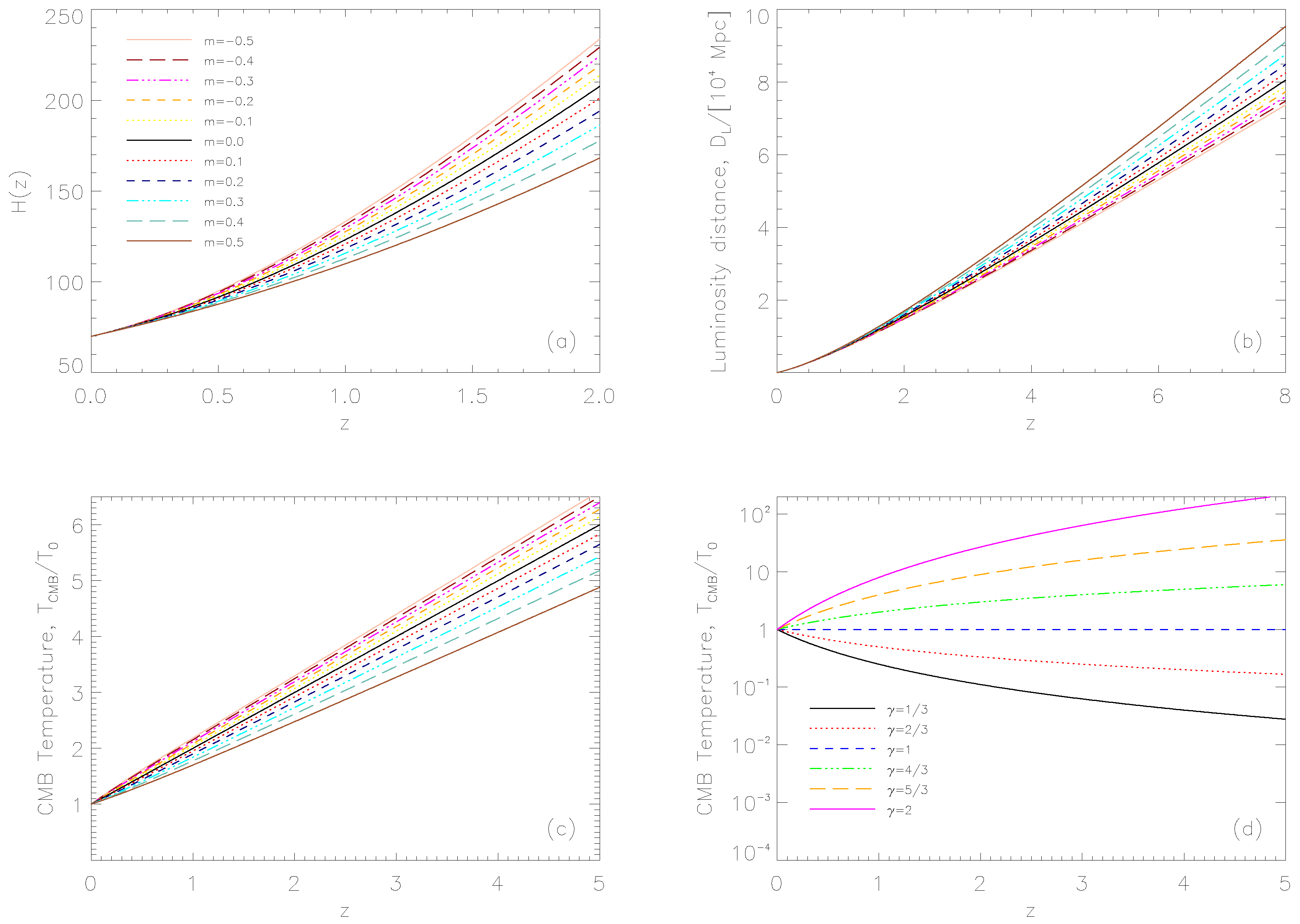
Figure 2.
2D marginalized contours of the model parameters obtained from the MCMC analysis. The 68% (dark grey) and 95% (light grey) confidence levels are shown for each pair of parameters. In each row, the marginalized likelihood distribution is also shown.
Figure 2.
2D marginalized contours of the model parameters obtained from the MCMC analysis. The 68% (dark grey) and 95% (light grey) confidence levels are shown for each pair of parameters. In each row, the marginalized likelihood distribution is also shown.
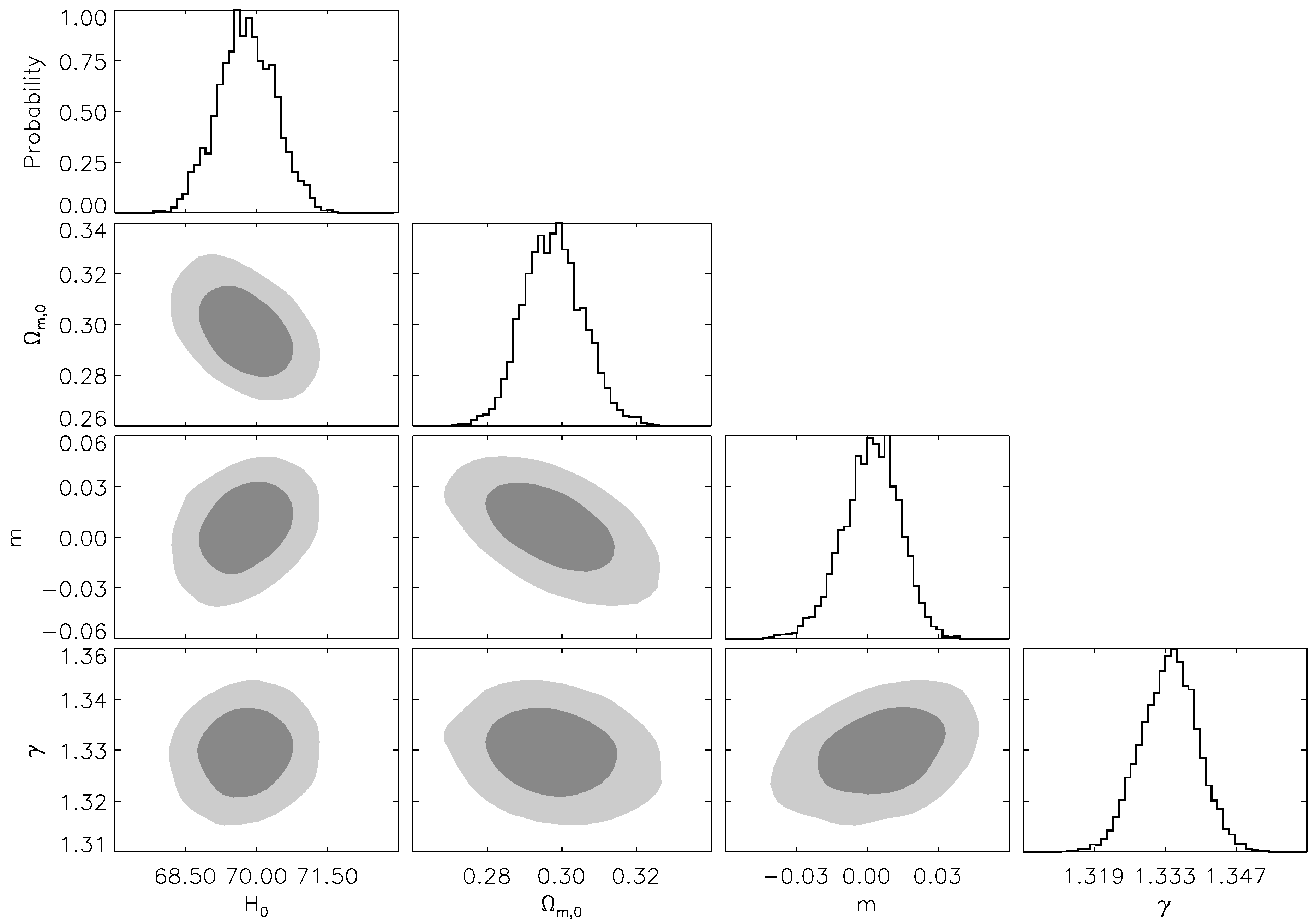
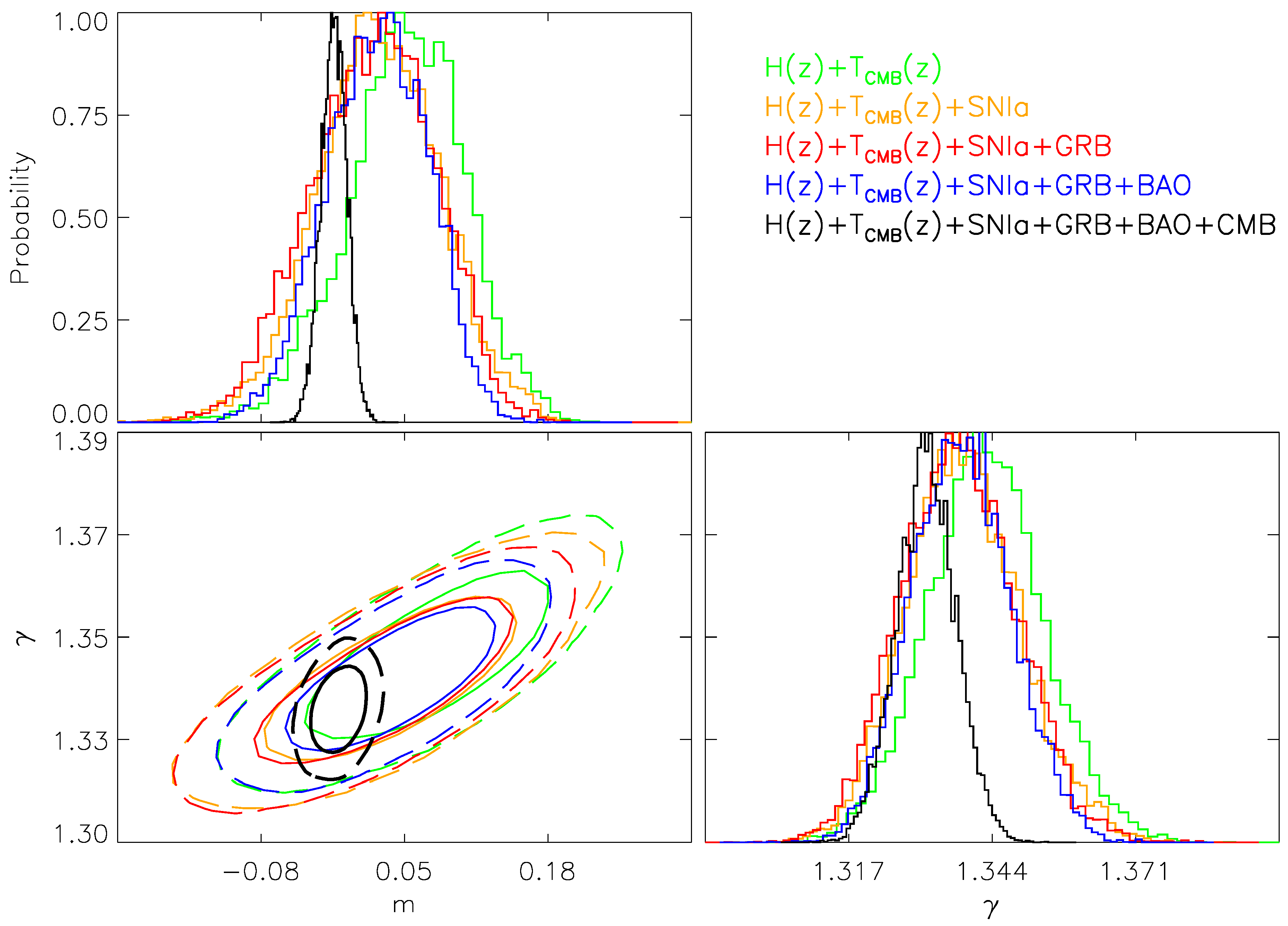
Figure 3.
2D marginalized 68% (solid line) and 95% (dashed line) contours of the model parameters obtained from the MCMC analysis.
Figure 3.
2D marginalized 68% (solid line) and 95% (dashed line) contours of the model parameters obtained from the MCMC analysis.


Table 1.
Parameter space explored by the MCMC algorithm.
| Parameter | Priors |
|---|---|
| m | [−1, 1] |
Table 2.
Maximum likelihood parameters and uncertainties from the MCMC algorithm and for the following datasets.
Table 2.
Maximum likelihood parameters and uncertainties from the MCMC algorithm and for the following datasets.
| Dataset | Free | |||
|---|---|---|---|---|
| + | ||||
| SNIa++ | ||||
| SNIa+GRB++ | ||||
| SNIa+GRB++BAO+ | ||||
| SNIa+GRB++BAO++CMB | ||||
| + | ||||
| SNIa++ | ||||
| SNIa+GRB++ | ||||
| SNIa+GRB++BAO+ | ||||
| SNIa+GRB++BAO++CMB | ||||
© 2018 by the author. Licensee MDPI, Basel, Switzerland. This article is an open access article distributed under the terms and conditions of the Creative Commons Attribution (CC BY) license (http://creativecommons.org/licenses/by/4.0/).
Share and Cite
MDPI and ACS Style
De Martino, I. Decaying Dark Energy in Light of the Latest Cosmological Dataset. Symmetry 2018, 10, 372. https://doi.org/10.3390/sym10090372
AMA Style
De Martino I. Decaying Dark Energy in Light of the Latest Cosmological Dataset. Symmetry. 2018; 10(9):372. https://doi.org/10.3390/sym10090372
Chicago/Turabian StyleDe Martino, Ivan. 2018. "Decaying Dark Energy in Light of the Latest Cosmological Dataset" Symmetry 10, no. 9: 372. https://doi.org/10.3390/sym10090372
Note that from the first issue of 2016, this journal uses article numbers instead of page numbers. See further details here.