A Linguistic Neutrosophic Multi-Criteria Group Decision-Making Method to University Human Resource Management

1
School of Business, Central South University, Changsha 410083, China
2
College of Business Administration, Hunan University, Changsha 410082, China
*
Author to whom correspondence should be addressed.
Symmetry 2018, 10(9), 364; https://doi.org/10.3390/sym10090364
Submission received: 17 July 2018
/
Revised: 11 August 2018
/
Accepted: 22 August 2018
/
Published: 26 August 2018
(This article belongs to the Special Issue Algebraic Structures of Neutrosophic Triplets, Neutrosophic Duplets, or Neutrosophic Multisets)
Abstract
:Competition among different universities depends largely on the competition for talent. Talent evaluation and selection is one of the main activities in human resource management (HRM) which is critical for university development. Firstly, linguistic neutrosophic sets (LNSs) are introduced to better express multiple uncertain information during the evaluation procedure. We further merge the power averaging operator with LNSs for information aggregation and propose a LN-power weighted averaging (LNPWA) operator and a LN-power weighted geometric (LNPWG) operator. Then, an extended technique for order preference by similarity to ideal solution (TOPSIS) method is developed to solve a case of university HRM evaluation problem. The main contribution and novelty of the proposed method rely on that it allows the information provided by different decision makers (DMs) to support and reinforce each other which is more consistent with the actual situation of university HRM evaluation. In addition, its effectiveness and advantages over existing methods are verified through sensitivity and comparative analysis. The results show that the proposal is capable in the domain of university HRM evaluation and may contribute to the talent introduction in universities.
1. Introduction
Human resource management (HRM) refers to a process of hiring and developing employees to enhance the core competitiveness of an organization [1]. Acting as the root of national competitiveness, a success in HRM may bring benefit to both the organization and employee well-being; thus, effective HRM has received a higher demand and recognition during the 21st century. Over the past three decades, theory and research on HRM has made considerable progress in various fields, such as tourism industries, health services and universities [2,3,4,5]. For example, Zhang et al. [5] investigated a case of HRM for teaching quality assessment using a multi-criteria group decision-making (MAGDM) framework. This framework aimed to improve the teaching quality of college teachers and further enhance the competitiveness of colleges and universities. Apart from the classroom teaching quality evaluation problems in universities, talent introduction also plays a significant role in universities’ HRM. Particularly, selecting or evaluating these applicants by inappropriate methods may lead to a failure in HRM and even influence the overall efficiency of the university. Since various applicants and influential criteria are usually involved in the evaluation procedures of HRM by several decision makers (DMs), the evaluation should be recognized as a multi-criteria group decision-making (MCGDM) problem.
The theory of fuzzy set (FS) can handle uncertainty and fuzziness. The neutrosophic set (NS) [6] was initially proposed to express membership, nonmembership and indeterminacy, which is a generalization of FS [7]. Later, many extensions emerged to tackle real engineering and scientific problems [8], among which the popularly used forms are the simplified neutrosophic set (SNS) [9] and the single-valued trapezoidal neutrosophic set (SVTNS) [10,11,12]. These extensions have been successfully applied in various domains, including green product development [13], outsourcing provider selection [14], clustering analysis [15,16].
However, on some real occasions, people may tend to provide their evaluation information using natural languages rather than the above extensions which are too complex to obtain. For example, people can give some linguistic terms like “excellent”, “medium” or “poor” to evaluate the performance of a company staff based on various criteria. Moreover, it may be also difficult for a single person to evaluate all alternatives under each influential aspect due to the high complexity of decision environments. Therefore, the linguistic MCGDM under fuzzy environments has received extensive research attention and gained many excellent results [17]. Up to now, various extensions have been studied in depth to describe linguistic information, such as hesitant fuzzy linguistic term set and some of its extended forms [18,19,20,21,22], linguistic intuitionistic fuzzy set (LIFS) [23,24], Z-number [25], and probabilistic linguistic term set [26,27] etc. However, the drawback of these extensions for linguistic MCGDM is that they cannot cover the inconsistent linguistic decision information which will appear with increasing complexity of the internal and external decision-making environments. Another example is that when one DM was asked to give some evaluations on a teacher from overseas under the aspect teaching skill, the DM may describe his or her bad judgments on the teaching attitude but the good or neutral aspects of the teacher’s teaching capacity and teaching method as well. An example of that can be seen from the evaluation: “The teacher is rather average in writing and oral language, and he is able to tailor his teaching method to different students. But my only complaint is that the teacher is a little strict in teaching attitude”. It can be noted that the above evaluation includes positive, neutral and negative information all at once. Therefore, this poses a great challenge for linguistic MCGDM methods on how to capture such inconsistent information.
To tackle the above problem, Fang and Ye [28] proposed the linguistic neutrosophic set (LNS), which was generalized from the concept of LIFS [23,24]. By contrast, one LNS is represented by three independent functions of truth-membership, indeterminacy-membership, and falsity-membership in the form of linguistic terms. Thus, the LNS has its prominent advantages in depicting inconsistent and indeterminate linguistic information, and several scholars have extended the LNS in several aspects, such as aggregation operators and similarity (or distance) measures. Li et al. [29] introduced a linguistic neutrosophic geometric Heronian mean (LNGHM) operator and a linguistic neutrosophic prioritized geometric Horonian mean (LNGHM) operator. Fan et al. [30] merged the LNSs with Bonferroni mean operator and proposed a linguistic neutrosophic number normalized weighted Bonferroni mean (LNNNWBM) operator and a linguistic neutrosophic number normalized weighted geometric Bonferroni mean (LNNNWGBM) operator. Shi and Ye [31] introduced two cosine similarity measures of LNSs to tackle MCGDM problems. Liang et al. [32] defined several distance measures of LNS and presented an extended TOPSIS method under the LNS environment.
To facilitate the mathematical operation, several quantification tools of natural language have been introduced, such as 2-type [33], triangular (or trapezoidal) fuzzy number [34,35], cloud model [36] and symbol model [37,38]. These models have greatly contributed to the ease of computation for linguistic information; however, they cannot cover all types of problems and have some limitations to be addressed. To tackle the limitations of prior research, Wang et al. [39] introduced a series of linguistic scale functions (LSFs) for converting linguistic information into real numbers. Through this model, flexibility of modeling information has been greatly enhanced by considering different semantic situations and loss and distortion of information has been mitigated to a great extent. Thus, we apply the LSFs to tackle linguistic neutrosophic information in this paper.
The power averaging (PA) operator, proposed by Yager [40], has been used as one effective information aggregation tool in solving MCDM [41,42,43] problems since its appearance. Unlike other common aggregation tools, such as weighted averaging [44] and ordered weighted averaging [45,46], which implicate the independent hypothesis among inputs. The PA operator allows the information between inputs to support and reinforce each other. In the HRM evaluation problems, it is very suitable for PA operator to integrate evaluation information of different teams of DMs, as these DMs are not completely independent and the PA operator can measure their support degree among one another.
TOPSIS method was first presented by Huang and Yoon [47]. It considered that the better scheme would be closer to ideal solution [48]. Due to the inevitable vagueness inherent in decision information, fuzzy TOPSIS and its extensions have been deployed [49,50,51] in real world applications. Considering the advantages of this method, an extended TOPSIS technique is introduced to evaluate alternatives.
As discussed above, our study developed an integrated method by combining PA operator with LNSs and constructing an extended TOPSIS technique to tackle the university HRM evaluation problem. The novelties and contributions of the proposal are listed as following. (1) New algorithms for LNNs based on LSFs is defined, which can reflect differences between various semantics. (2) Based on LSFs and the new operations, a generalized distance measure for LNNs is introduced, which can be reduced to Hamming distance and Euclidean distance of LNNs. The proposed distance measure is more flexible than prior studies because of the application of LSFs and novel operations. (3) Considering the fact that DMs in case of university HRM evaluation may support each other, this paper merges the PA operator with LNSs to tackle information fusion. The proposed method can improve the adaptability of LNNs in real decision.
The context in the rest of this paper is as follows: Section 2 defines some operations and distance measurements of LNSs. Section 3 proposes two aggregation operators for LNSs and investigates their properties. Next, the detailed procedures for a linguistic MCGDM problem are given in Section 4. Then, a case of university HRM evaluation problem verifies the feasibility and validity of our method in Section 5. Finally, Section 6 presents the conclusion and future work.
2. New Operations and Distance Measure for LNNs
After introducing the concepts of linguistic term set (LTS) and LNS, this section defines some new operations and a distance measure for LNNs based on the Archimedean t-norm and t-conorm. For better representation, some preliminaries about LSFs and the Archimedean t-norm and t-conorm are provided in Appendix A and Appendix B, respectively.
2.1. Linguistic Neutrosophic Set
is a discrete term set, which is finite and totally ordered. Herein, presents a positive integers’ set, is the value of a linguistic variable. Thus, the linguistic variable in meets the following two properties [34]: (1) The LTS is ordered: if and only if , where ; and (2) With existing of a negation operator .
In order to preserve as much of the given information and avoid information loss, Xu [52] extended into a continuous LTS , which satisfies the properties of discrete term set . When , is called the original linguistic term; otherwise, is called the virtual linguistic term.
Definition 1
Noteworthy, if there contains only one element in , is called a LNN, for notational simplicity, it can be denoted by .
2.2. New Operations for LNNs
According to the LSFs in Appendix A and the Archimedean t-norm and t-conorm presented in Appendix B, some novel operations for LNNs are defined as follows.
Definition 2.
Letandbe two arbitrary LNNs, and; then the operations for LNNs are defined as follows:
- (1)
- ;
- (2)
- ;
- (3)
- ;
- (4)
- ; and
- (5)
- .
Example 1.
Let , , , and , if , and . The calculated results are as follows:
- (1)
- ;
- (2)
- ;
- (3)
- ; and
- (4)
- .
Theorem 1.
Let,, andbe three LNNs, and; then the following equations are true:
- (1)
- ;
- (2)
- ;
- (3)
- ;
- (4)
- ;
- (5)
- ; and
- (6)
- .
Theorem 1 holds according to Definition 2, so the proof is omitted here.
2.3. Distance between Two LNNs
Definition 3.
Letandbe two arbitrary LNNs,is a LSF. Then, the generalized distance measure betweenandis defined as follows:
When, the above distance measure can be reduced to the Hamming distance; when, it can be reduced to the Euclidean distance. We can see that Equation (2) is a generalized form of distance measure.
Theorem 2.
Let,andbe three arbitrary LNNs, then, the following properties are required for the generalized distance measure in Definition 3.
- (1)
- ;
- (2)
- ;
- (3)
- ; and
- (4)
- .
Theorem 2 is proved in the Appendix C for better representation.
3. Linguistic Neutrosophic Aggregation Operators
Yager [40] introduced the PA operator to allow input arguments to support each other. Thus, the traditional PA operator are first reviewed; then, the LNPWA and LNPWG operators are proposed in an environment featuring LNNs.
Definition 4
([40]). Let be a collection of positive values and be the set of all given values; then the PA operator is the mapping , which can be defined as follows:
where
represents the support forfrom, and meets the following properties:
- (1)
- ;
- (2)
- ; and
- (3)
- , when, andis the distance betweenand.
3.1. Linguistic Neutrosophic Power Weighted Averaging Operator
This subsection extends the traditional PA operator to LNN. Then, a LNPWA operator is proposed and discussed.
Definition 5.
Letbe a set of LNNs. Then, the LNPWA operator can be defined as
whereis the weight vector of,, and,,is the support forfrom, which also satisfies the similar properties in Definition 4.
Theorem 3.
Letbe a set of LNNs, andis the weight vector of,, and. Then, the aggregated result using Equation (5) is also a LNN. For notational simplicity, we assume that.
“Appendix D” details the proof of Theorem 3.
The traditional PA operator has the properties of idempotency, monotonicity, and boundedness. It can be proved that the LNPWA operator also satisfies these properties.
Theorem 4.
Letbe a set of LNNs, andis the weight vector of,, and. Iforfor alland. Hence, the LNPWA operator reduces to the linguistic neutrosophic weighted averaging (LNWA) operator.
The proof for Theorem 4 is similar to the proof for Theorem 3; thus, it is omitted here.
3.2. Linguistic Neutrosophic Power Weighted Geometric Operator
Definition 6.
Letbe a set of LNNs. Then, the LNPWG operator can be defined as
whereis the weight vector of,, and,,is the support forfromand also satisfies the properties in Definition 4.
Theorem 5.
Letbe a set of LNNs, andis the weight vector of,, and. Then, the aggregated result using Equation (8) is still a LNN, For notational simplicity, we assume that.
The proof of Theorem 5 is also omitted duo to the same way as Theorem 3.
4. MCGDM Method Based on the LNPWA and LNPWG Operators
In this part, a MCGDM method based on the LNPWA and LNPWG operators is developed to solve university HRM evaluation problems.
For a MCGDM problem with a finite set of m alternatives, let be the set of DMs, be the set of alternatives, and be the set of criteria. Assume that the weight vector of the criteria is , such that and . Analogously, the weight vector of the DMs is specified as , where and . The evaluation values provided by the DMs are transformed into LNNs, and , represents the evaluation value of DM for alternative on criteria .
The detailed procedures of the MCGDM method involve the following steps:
Step 1: Normalize the decision matrices.
In general, criteria can be divided into two categories: benefit type and cost type. Using operation (5) in Definition 2, the cost criteria can be transformed into benefit ones as follows:
Step 2: Obtain the weighted decision matrices.
Using operations in Definition 2, the weighted decision matrices can be constructed by multiplying the given criteria weight vector into the decision matrices.
Step 3: Calculate the supports.
Utilizing the distance measure defined in Definition 3, the support degrees can be obtained by Equation (11):
Step 4: Calculate the weights associated with .
where , and is interpreted as the weight of DM .
Step 5: Obtain the comprehensive evaluation information.
Using Equation (5) or Equation (9), the normalized evaluation information provided by DMs can be aggregated, and the integrated decision matrix can be obtained.
Step 6: Determine the ideal decision vectors of all alternative decisions.
After aggregating the DMs’ evaluation information into the decision matrix , which is as follow:
We can determine the ideal alternative vector among all the alternatives below:
Similarly, the negative ideal alternative vector can be obtained by the negation of , which has the maximum separation from , as follows:
In addition, we can obtain the left maximum separation from denoted as :
where , , and .
In the same way, we can also obtain the right maximum separation from denoted as :
where , , and .
Step 7: Calculate the separations of each alternative decision vector from the ideal decision vector.
Utilizing the distance measure in Definition 3, we can calculate the separations between each alternative vector and the ideal decision vectors of all alternative decisions, they are respectively represented as follows:
Step 8: Calculate the relative closeness of each alternative decision.
The relative closeness of each alternative decision can be obtained using the following formula:
Step 9: Rank all the alternatives.
According to the relative closeness of each alternative decision , we can rank all the alternatives. The larger the value of , the better the alternative is.
5. A Case of Human Resource Management Problem
5.1. Problem Definition
The present study focuses on a case of HRM problem in a Chinese university to test the proposed MCGDM method. Specifically, the school of management in the university plans to introduce talents from home and abroad to strengthen discipline construction and try to realize the goal of building a high-level innovative university. Three teams of DMs are assembled as a committee and will take the whole responsibility for this recruitment process, these teams are university presidents , deans of management school , and human resource officers , respectively. After strict first interview, six candidates remain for the second review. Before the evaluation procedures, an appropriate evaluation index system should be constructed through literature review and expert consultation. In the literature research, Abdullah et al. [1] and Chou et al. [53] identified three dimensions and eight criteria for the HRM evaluation problem; the three dimensions used in their work were infrastructures, input and output. Zhang et al. [5] constructed an evaluation index system of classroom teaching quality; dimensions included in their work were usage of teaching attitude, teaching capacity, teaching content, teaching method and teaching effect. We can see that different evaluation index systems serve for different purposes of HRM evaluation in various industries. This study mainly tackles the HRM evaluation for talent introduction in universities which exists in real-life decision environments. According to Ref. [54], experts agree on the four criteria included in the evaluation index system for the evaluation of HRM, they are teaching skill (), morality (), education background () and research capability (), respectively. A brief description of each criterion is shown as follows.
Teaching skill is an overall reflect of one teacher’s classroom teaching quality which includes several sub-attributes, such as teaching attitude, teaching capacity, teaching content, teaching method and teaching effect.
Morality refers to the teachers’ morality in this study. It is a kind of professional morality of teachers which takes up the first place of education and can greatly affects the education’s level and quality as a whole. More specifically, the teachers’ morality includes the moral consciousness, moral relations and moral activity of the teachers in universities.
Education background is an overview of a person’s learning environment and learning ability. It includes the person’s educational level, graduate school, major courses, academic achievements, and some other highlights.
Research capability denotes the scientific research ability that is required for scientific research or the research competence someone shows during the process of scientific research. The former is closer to the potential, including someone’s abilities in logical thinking, writing and oral language, etc., whereas the latter emphasizes someone’s practical scientific research capacity.
With the reform of education and fierce competition among universities, the current form of university education needs more and more modern teachers with the above four abilities. Therefore, this study applies the above four criteria for the case of HRM evaluation, and the six candidates are evaluated by the three teams of DMs under each criterion. The weight vector of criteria was assigned by DMs as , and the weight vector of DMs was . In addition, the LTS was denoted as . By interviewing the DMs one by one anonymously, all of their linguistic assessments for each alternative under each criterion are collected together. During this process, DMs in each group are isolated and don’t negotiate with each other at all. Consequently, the decision information is provided independently in the form of linguistic terms. Take the evaluation value as an example, which represents the evaluation value of DM for alternative under criterion . Since the criterion (teaching skill) includes various aspects, such as teaching attitude, teaching capacity, teaching content, teaching method and teaching effect, the group of DMs may hold inconsistent linguistic judgments for alternative with respect to . After collecting all the linguistic assessments for alternative , the linguistic neutrosophic information is obtained by calculating the weighted mean values of all the labels of linguistic terms with respect to active, neutral and passive information, respectively. Similarly, the overall evaluation information provided by the teams of DMs can be represented in the form of LNNs in Table 1, Table 2 and Table 3.
5.2. Evaluation Steps of the Proposed Method
The following steps describe the procedures of evaluation for all candidates, and the ranking order of the six alternatives can be obtained. For simplicity of calculation, we chose the LSF .
Step 1: Normalize the decision matrices.
It is obvious that all the four criteria are of the benefit type; then, there is no need for normalization.
Step 2: Obtain the weighted decision matrices.
Using operation in Definition 2, the weighted decision matrices can be constructed in Table 4, Table 5 and Table 6:
Step 3: Calculate the supports.
Utilizing the distance measure defined in Definition 3 and Equation (11), the supports can be obtained. Here, we assume that in the distance measure.
,
, and
Step 4: Calculate the weights associated with .
The weights can be calculated by Equation (12) as follows:
, , and
Step 5: Obtain the comprehensive evaluation information.
Using Equation (5) or Equation (9), the integrated decision matrix are calculated below:
(i) When using Equation (5), the results are listed in Table 7.
(ii) When using Equation (9), the results are listed in Table 8.
Step 6: Determine the ideal decision vectors of all alternative decisions.
(i) When using Equation (5), we can determine the ideal alternative vectors among all the alternatives respectively as follows:
,
,
, and
.
(ii) When using Equation (9), the results are:
,
,
, and
.
Step 7: Calculate the separations of each alternative decision vector from the ideal decision vector.
The separations between each alternative and the ideal decision vector by the LNPWA and LNPGA operators are shown in Table 9 and Table 10, respectively.
Step 8: Calculate the relative closeness of each alternative decision.
The results of relative closeness of each alternative decision are shown in the last column of Table 9 and Table 10.
Step 9: Rank all the alternatives.
According to the relative closeness of each alternative decision , we can rank all the alternatives. When using LNPWA operator, the ranking result is , whereas when using LNPWG operator, the result turns out . There is a subtle distinction between the results obtained by the LNPWA and LNPWG operators, but the alternative remains the most performant and competitive candidate.
5.3. Sensitivity Analysis and Discussion
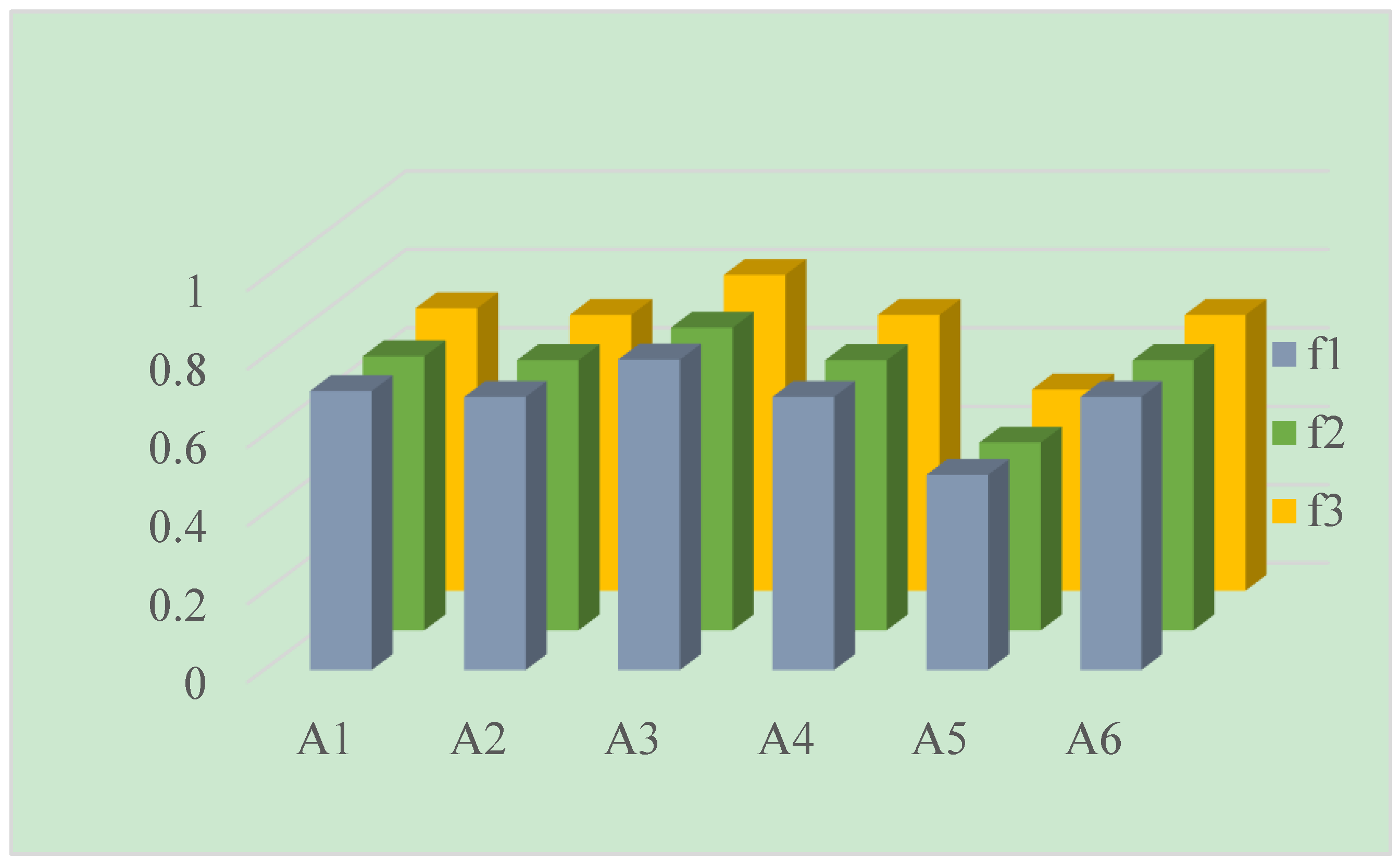
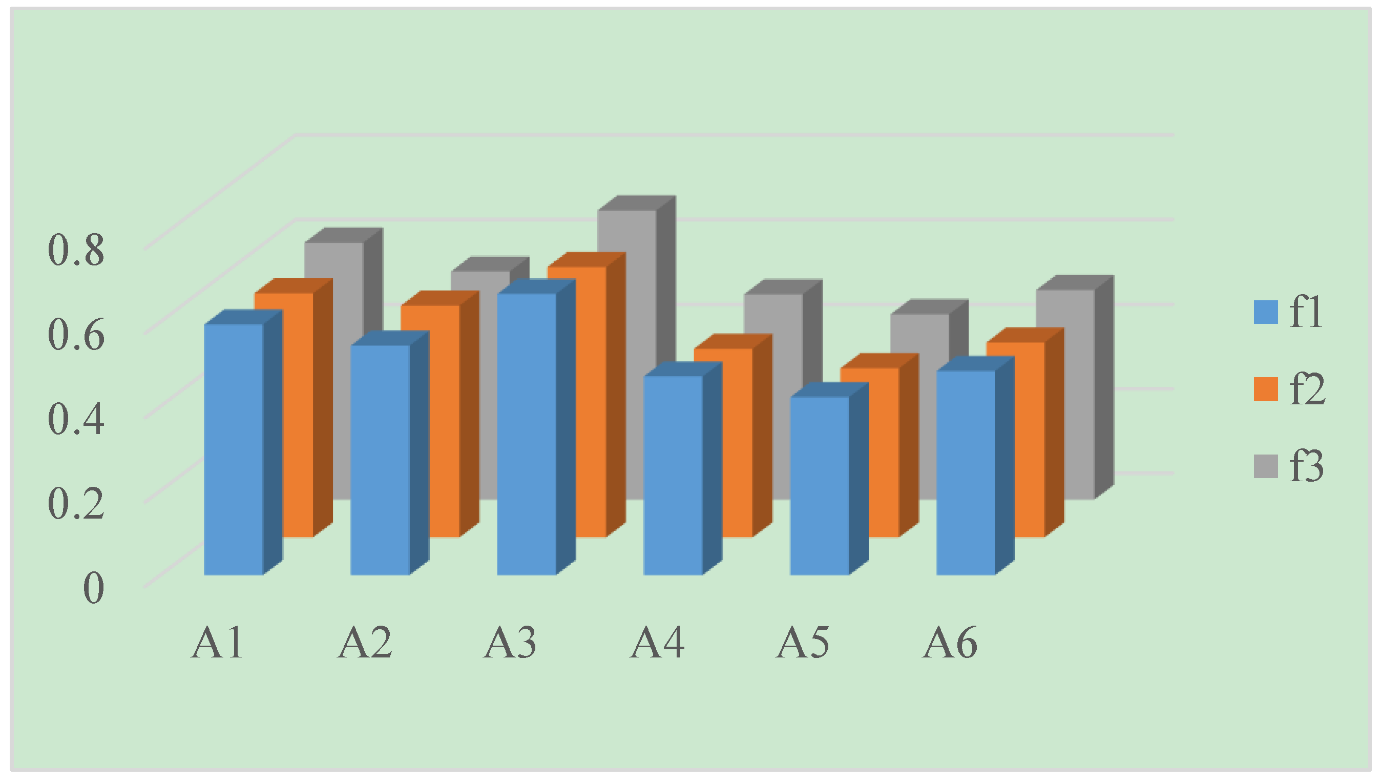
The aim of sensitivity analysis is to investigate the effects of different semantics and the distance parameter on the final ranking results of alternatives. To do so, the calculated results are shown in Table 11 and Table 12 and Figure 1 and Figure 2, respectively.
It can be seen from Table 11 and Figure 1 and Figure 2 that the alternative remained to be the best one, and was consistently identified as the worst choice no matter how the aggregation operator or semantics change. When using the LNPWA operator, the ranking result remains . The difference in semantics slightly influenced the values of , but did not result in different ranking orders. Similarly, when using the LNPWG operator, the ranking result always is . It is clear that the ranking results varied when using different aggregation operators. This may be caused by the distinct inherent characteristic of these two operators, since the LNPWA operator is based on the arithmetic averaging, whereas the LNPWG operator is based on the geometric averaging. This demonstrates that the ranking results have stability by our proposed method in some degree.
The following Table 12 the influence of the distance parameter on the final ranking results of alternatives when the semantics were fixed as . It can be seen that the ranking results kept the same as when using the LNPWG operator. However, results by the LNPWA operator change among , and . Thus, we can conclude that the differences in the aggregation operators and the parameter could influence the evaluation results, DMs should choose appropriate parameter and aggregation operators according to their own inherent characteristics.
5.4. Comparison Analysis and Discussion
This subsection conducts a comparative study to validate the practicality and advantages of the proposed method in the LNS contexts, and the results are shown in Table 13. Brief descriptions about the comparative methods are as follows.
(1) Weighted arithmetic and geometric averaging operators of LNNs [28]: the concept of LNNs was first proposed by Fang and Ye [28]. In their study, two aggregation operators including the LNN-weighted arithmetic averaging (LNNWAA) operator and LNN-weighted geometric averaging (LNNWGA) operator are utilized to derive collective evaluations. Then, based on their proposed score function and accuracy function of LNNs, the ranking order of alternatives is obtained.
(2) Bonferroni mean operators of LNNs [30]: the LNNNWBM operator and LNNNWGBM operator are proposed to aggregate evaluations to obtain the collective LNN for each alternative. Subsequently, the results are derived by expected value.
(3) An extended TOPSIS method [32]: a weighted model based on maximizing deviation is used to determine criteria weights. Subsequently, an extended TOPSIS method with LNNs is proposed to rank alternatives.
As shown in Table 13, different methods resulted in different ranking results, but the optimal candidate remained to be , despite the results obtained by the Bonferroni mean operators of LNNs [30]. The main reasons for these differences may be as follows: (1) The operations for LNNs between this study and the comparative methods are remarkably different. The operations in the existing methods [28,30,32] just considered the linguistic variables’ labels which may cause information loss and distortion. (2) Different aggregation operators and ranking rules might also cause different ranking results. Specifically, the LNNWAA and LNNWGA operators defined in [28] were respectively based on the arithmetic mean and geometric mean operators, whereas the Bonferroni mean operators of LNNs [30] implicated the interactive hypothesis among inputs. Unlike the existing aggregation tools, the proposed PA operator for LNNs allows the information provided by different DMs to support and reinforce each other, and it is a nonlinear weighted average operator.
From above discussions, the unique features of the proposal and its main advantages over others can be simply summarized below.
(1) The comparative methods [28,30,32] dealt with the LNNs only considering the labels of linguistic variables while ignoring the differences in various semantics. It has been contended that the same linguistic variable possesses different meanings for different people and has diverse meanings for the same person under various situations [55]. Therefore, directly using the labels of linguistic variables may lead to information loss during information aggregation. To cover this challenge, this study redefines the operations for LNNs based on the LSFs and Archimedean t-norm and t-conorm, which increases the flexibility and accuracy of linguistic information transformation.
(2) The extended TOPSIS method [32] only considered two relatively positive and negative ideal solutions to determine the values of correlation coefficient for each alternative. By contrast, this study takes both the relatively and absolutely positive and negative ideal solutions into account. Therefore, the ranking result by this proposed method may be somewhat more comprehensive than the existing method [32].
(3) For information fusion, all the existing methods [28,30,32] failed to consider the support degree among different DMs during the aggregation processes. Although it is true that different aggregation operators cater to different practical decision situations, the proposed PA operators within LNN contexts are more feasible in dealing with the university HRM evaluation problem in this study.
6. Conclusions and Future Work
Talent introduction plays an important role in the long-term development of a university. This is closely related to the university’s discipline development and comprehensive strength. Therefore, there is a need for proper HRM evaluation that uses group decision-making methods efficiently in order to utilize human resources. This study recognized the HRM evaluation procedures as a complex MCGDM problems within the LNNs’ circumstances. Through merging the PA operator with LNSs, we developed two aggregation operators (LNPWA and LNPWG) for information fusion. Then, we made some modifications in the classical TOPSIS method to determine the ranking order of alternatives. The strengths of the proposed method have been discussed via comparative analysis.
Nevertheless, this study also holds several limitations which can suggest several avenues for future research. First, the information fusion process adds to the computational complexity of the obtained results because the proposed LNPWA and LNPWG operators are both nonlinear weighted average operators, where the weights associated with each DM should be calculated by their input arguments. Fortunately, the pressure from complex computation can be remarkably eased with the assistance of programming software. Second, with the rapid development of information technology, it is also possible to extend the current results for other management systems under the network-based environments [56,57].
By analyzing the achieved results, the practical implications of our research may be summarized in two aspects. On the one hand, this study proposes a novel linguistic neutrosophic MCGDM method which contributes to expanding the theoretical depth of university HRM. It may offer comprehensive supports for decision-making of modern universities’ talent introduction. In addition, the developed method can also be further expanded to solving group decision-making problems in other fields, such as tourism. On the other hand, this study further explores the application of linguistic MCGDM methods in HRM. The obtained knowledge can be very helpful to improve the performance of the human resource of universities accordingly.
Author Contributions
R.-x.L., J.-q.W. and Z.-b.J. conceived and worked together to achieve this work; and R.-x.L. and Z.-b.J. wrote the paper.
Funding
This research was funded by Fundamental Research Funds for the Central Universities of Central South University grant number (No. 502211710), and the APC was also funded by (No. 502211710).
Acknowledgments
The authors would like to thank the editors and anonymous reviewers for their great help on this study.
Conflicts of Interest
The authors declare no conflict of interest.
Appendix A. Linguistic Scale Function
By means of literature review, we can gather the following choices acting as LSFs.
(1) The LSF is based on the subscript function :
The above function is divided on average. It is commonly used for its simple form and easy calculation, but it lacks a reasonable theoretical basis [58].
(2) The LSF is based on the exponential scale:
Here, the absolute deviation between any two adjacent linguistic labels decreases with the increase of in the interval , and increases with the increase of in the interval .
(3) The LSF is based on prospect theory:
Here, , and when , the LSF is reduced to . Moreover, the absolute deviation between any two adjacent linguistic labels increases with the increase of in the interval , and decreases with the increase of in the interval .
Each of the above LSFs , , and can be expanded to a strictly monotonically increasing and continuous function: , which satisfies . Therefore, the inverse function of , denoted as , exists due to its monotonicity.
Appendix B. The Archimedean T-norm and T-conorm
According to Reference [59], a t-norm is called Archimedean t-norm if it is continuous and , for all . An Archimedean t-norm is called a strict Archimedean t-norm if it is strictly increasing in every variable for . In addition, a t-conorm is called Archimedean t-conorm if it is continuous and , for all . An Archimedean t-conorm is called a strict Archimedean t-conorm if it is strictly increasing in every variable for .
Appendix C. The Proof of Theorem 2
Proof.
It is clear that properties (1)–(3) in Theorem 2 hold. The proof of property (4) in Theorem 2 is shown below.
First, the distances , and can be easily determined respectively as follows:
,
, and
.
Since , then , and
.
Thus, .
Similarly, we can obtain , and .
Then
Thus, property (4) in Theorem 2 holds. □
Appendix D. The Proof of Theorem 3
For ease of computation, we assume that . In the following steps, Equation (5) will be proven using mathematical induction on .
(1) Utilizing the operations for LNNs defined in Definition 2, when , we have
That is
Thus, when , Equation (5) is true.
(2) Suppose that when , Equation (5) is true. That is,
Then, when , the following result can be obtained:
Then, when , Equation (5) is true. Therefore, Equation (5) is true for all .
References
- Abdullah, L.; Zulkifli, N. Integration of fuzzy AHP and interval type-2 fuzzy DEMATEL: An application to human resource management. Expert Syst. Appl. 2015, 42, 4397–4409. [Google Scholar] [CrossRef]
- Filho, C.F.F.C.; Rocha, D.A.R.; Costa, M.G.F. Using constraint satisfaction problem approach to solve human resource allocation problems in cooperative health services. Expert Syst. Appl. 2012, 39, 385–394. [Google Scholar] [CrossRef]
- Marcolajara, B.; ÚbedaGarcía, M. Human resource management approaches in Spanish hotels: An introductory analysis. Int. J. Hosp. Manag. 2013, 35, 339–347. [Google Scholar] [CrossRef]
- Bohlouli, M.; Mittas, N.; Kakarontzas, G.; Theodosiou, T.; Angelis, L.; Fathi, M. Competence assessment as an expert system for human resource management: A mathematical approach. Expert Syst. Appl. 2017, 70, 83–102. [Google Scholar] [CrossRef]
- Zhang, X.; Wang, J.; Zhang, H.; Hu, J. A heterogeneous linguistic MAGDM framework to classroom teaching quality evaluation. Eurasia J. Math. Sci. Technol. Educ. 2017, 13, 4929–4956. [Google Scholar] [CrossRef]
- Smarandache, F. A Unifying Field in Logics: Neutrosophic Logic: Neutrosophy, Neutrosophic Set, Neutrosophic Probability; American Research Press: Rehoboth, DE, USA, 1999; pp. 1–141. [Google Scholar]
- Zadeh, L.A. Fuzzy sets. Inf. Control 1965, 8, 338–353. [Google Scholar] [CrossRef] [Green Version]
- Wu, X.H.; Wang, J.Q.; Peng, J.J.; Qian, J. A novel group decision-making method with probability hesitant interval neutrosphic set and its application in middle level manager’ selection. Int. J. Uncertain. Quantif. 2018, 8, 291–319. [Google Scholar] [CrossRef]
- Ji, P.; Wang, J.Q.; Zhang, H.Y. Frank prioritized Bonferroni mean operator with single-valued neutrosophic sets and its application in selecting third-party logistics providers. Neural Comput. Appl. 2016, 30, 799–823. [Google Scholar] [CrossRef]
- Liang, R.; Wang, J.; Zhang, H. Evaluation of e-commerce websites: An integrated approach under a single-valued trapezoidal neutrosophic environment. Knowl.-Based Syst. 2017, 135, 44–59. [Google Scholar] [CrossRef]
- Liang, R.X.; Wang, J.Q.; Zhang, H.Y. A multi-criteria decision-making method based on single-valued trapezoidal neutrosophic preference relations with complete weight information. Neural Comput. Appl. 2017. [Google Scholar] [CrossRef]
- Liang, R.X.; Wang, J.Q.; Li, L. Multi-criteria group decision making method based on interdependent inputs of single valued trapezoidal neutrosophic information. Neural Comput. Appl. 2018, 30, 241–260. [Google Scholar] [CrossRef]
- Tian, Z.P.; Wang, J.; Wang, J.Q.; Zhang, H.Y. Simplified neutrosophic linguistic multi-criteria group decision-making approach to green product development. Group Decis. Negot. 2017, 26, 597–627. [Google Scholar] [CrossRef]
- Ji, P.; Zhang, H.Y.; Wang, J.Q. Selecting an outsourcing provider based on the combined MABAC–ELECTRE method using single-valued neutrosophic linguistic sets. Comput. Ind. Eng. 2018, 120, 429–441. [Google Scholar] [CrossRef]
- Karaaslan, F. Correlation coefficients of single-valued neutrosophic refined soft sets and their applications in clustering analysis. Neural Comput. Appl. 2017, 28, 2781–2793. [Google Scholar] [CrossRef]
- Ye, J. Single-valued neutrosophic clustering algorithms based on similarity measures. J. Classif. 2017, 34, 148–162. [Google Scholar] [CrossRef]
- Li, Y.Y.; Wang, J.Q.; Wang, T.L. A linguistic neutrosophic multi-criteria group decision-making approach with EDAS method. Arab. J. Sci. Eng. 2018. [Google Scholar] [CrossRef]
- Chen, Z.S.; Chin, K.S.; Li, Y.L.; Yang, Y. Proportional hesitant fuzzy linguistic term set for multiple criteria group decision making. Inf. Sci. 2016, 357, 61–87. [Google Scholar] [CrossRef]
- Rodríguez, R.M.; Martínez, L.; Herrera, F. Hesitant fuzzy linguistic term sets for decision making. IEEE Trans. Fuzzy Syst. 2012, 20, 109–119. [Google Scholar] [CrossRef]
- Wang, H. Extended hesitant fuzzy linguistic term sets and their aggregation in group decision making. Int. J. Comput. Intell. Syst. 2014, 8, 14–33. [Google Scholar] [CrossRef]
- Wang, X.K.; Peng, H.G.; Wang, J.Q. Hesitant linguistic intuitionistic fuzzy sets and their application in multi-criteria decision-making problems. Int. J. Uncertain. Quantif. 2018, 8, 321–341. [Google Scholar] [CrossRef]
- Tian, Z.P.; Wang, J.Q.; Zhang, H.Y.; Wang, T.L. Signed distance-based consensus in multi-criteria group decision-making with multi-granular hesitant unbalanced linguistic information. Comput. Ind. Eng. 2018, 124, 125–138. [Google Scholar] [CrossRef]
- Zhang, H.M. Linguistic intuitionistic fuzzy sets and application in MAGDM. J. Appl. Math. 2014, 2014. [Google Scholar] [CrossRef]
- Chen, Z.C.; Liu, P.H.; Pei, Z. An approach to multiple attribute group decision making based on linguistic intuitionistic fuzzy numbers. Int. J. Comput. Intell. Syst. 2015, 8, 747–760. [Google Scholar] [CrossRef] [Green Version]
- Peng, H.G.; Wang, J.Q. A multicriteria group decision-making method based on the normal cloud model with Zadeh’s Z-numbers. IEEE Trans. Fuzzy Syst. 2018. [Google Scholar] [CrossRef]
- Peng, H.G.; Zhang, H.Y.; Wang, J.Q. Cloud decision support model for selecting hotels on TripAdvisor.com with probabilistic linguistic information. Int. J. Hosp. Manag. 2018, 68, 124–138. [Google Scholar] [CrossRef]
- Luo, S.Z.; Zhang, H.Y.; Wang, J.Q.; Li, L. Group decision-making approach for evaluating the sustainability of constructed wetlands with probabilistic linguistic preference relations. J. Oper. Res. Soc. 2018. [Google Scholar] [CrossRef]
- Fang, Z.B.; Ye, J. Multiple attribute group decision-making method based on linguistic neutrosophic numbers. Symmetry 2017, 9, 111. [Google Scholar] [CrossRef]
- Li, Y.Y.; Zhang, H.Y.; Wang, J.Q. Linguistic neutrosophic sets and their application in multicriteria decision-making problems. Int. J. Uncertain. Quantif. 2017, 7, 135–154. [Google Scholar] [CrossRef]
- Fan, C.X.; Ye, J.; Hu, K.L.; Fan, E. Bonferroni mean operators of linguistic neutrosophic numbers and their multiple attribute group decision-making methods. Information 2017, 8, 107. [Google Scholar] [CrossRef]
- Shi, L.L.; Ye, J. Cosine measures of linguistic neutrosophic numbers and their application in multiple attribute group decision-making. Information 2017, 8, 117. [Google Scholar]
- Liang, W.Z.; Zhao, G.Y.; Wu, H. Evaluating investment risks of metallic mines using an extended TOPSIS method with linguistic neutrosophic numbers. Symmetry 2017, 9, 149. [Google Scholar] [CrossRef]
- Herrera, F.; Martínez, L. A 2-tuple fuzzy linguistic representation model for computing with words. IEEE Trans. Fuzzy Syst. 2000, 8, 746–752. [Google Scholar]
- Delgado, M.; Verdegay, J.L.; Vila, M.A. Linguistic decision-making models. Int. J. Intell. Syst. 1992, 7, 479–492. [Google Scholar] [CrossRef]
- Hu, J.; Zhang, X.; Yang, Y.; Liu, Y.; Chen, X. New doctors ranking system based on VIKOR method. Int. Trans. Oper. Res. 2018. [Google Scholar] [CrossRef]
- Li, D.Y.; Meng, H.J.; Shi, X.M. Membership clouds and membership cloud generators. Comput. Res. Dev. 1995, 32, 16–21. [Google Scholar]
- Bordogna, G.; Fedrizzi, M.; Pasi, G. A linguistic modeling of consensus in group decision making based on OWA operators. IEEE Trans. Syst. Man Cybern.-Part A Syst. Hum. 1997, 27, 126–133. [Google Scholar] [CrossRef]
- Doukas, H.; Karakosta, C.; Psarras, J. Computing with words to assess the sustainability of renewable energy options. Expert Syst. Appl. 2010, 37, 5491–5497. [Google Scholar] [CrossRef]
- Wang, J.Q.; Wu, J.T.; Wang, J.; Zhang, H.Y.; Chen, X.H. Interval-valued hesitant fuzzy linguistic sets and their applications in multi-criteria decision-making problems. Inf. Sci. 2014, 288, 55–72. [Google Scholar] [CrossRef]
- Yager, R.R. The power average operator. IEEE Trans. Syst. Man Cybern.-Part A Syst. Hum. 2001, 31, 724–731. [Google Scholar] [CrossRef]
- Jiang, W.; Wei, B.; Zhan, J.; Xie, C.; Zhou, D. A visibility graph power averaging aggregation operator: A methodology based on network analysis. Comput. Ind. Eng. 2016, 101, 260–268. [Google Scholar] [CrossRef]
- Gong, Z.; Xu, X.; Zhang, H.; Aytun Ozturk, U.; Herrera-Viedma, E.; Xu, C. The consensus models with interval preference opinions and their economic interpretation. Omega 2015, 55, 81–90. [Google Scholar] [CrossRef]
- Liu, P.D.; Qin, X.Y. Power average operators of linguistic intuitionistic fuzzy numbers and their application to multiple-attribute decision making. J. Intell. Fuzzy Syst. 2017, 32, 1029–1043. [Google Scholar] [CrossRef]
- Yager, R.R. Applications and extensions of OWA aggregations. Int. J. Man-Mach. Stud. 1992, 37, 103–132. [Google Scholar] [CrossRef]
- Yager, R.R. On ordered weighted averaging aggregation operators in multicriteria decision making. IEEE Trans. Syst. Man Cybern. 1988, 18, 183–190. [Google Scholar] [CrossRef]
- Yager, R.R. Families of OWA operators. Fuzzy Sets Syst. 1993, 59, 125–148. [Google Scholar] [CrossRef]
- Huang, J.J.; Yoon, K. Multiple Attribute Decision Making: Methods and Applications; Chapman and Hall/CRC: Boca Raton, FL, USA, 2011. [Google Scholar]
- Baykasoğlu, A.; Gölcük, İ. Development of an interval type-2 fuzzy sets based hierarchical MADM model by combining DEMATEL and TOPSIS. Expert Syst. Appl. 2017, 70, 37–51. [Google Scholar] [CrossRef]
- Joshi, D.; Kumar, S. Interval-valued intuitionistic hesitant fuzzy Choquet integral based TOPSIS method for multi-criteria group decision making. Eur. J. Oper. Res. 2016, 248, 183–191. [Google Scholar] [CrossRef]
- Mehrdad, A.M.A.K.; Aghdas, B.; Alireza, A.; Mahdi, G.; Hamed, K. Introducing a procedure for developing a novel centrality measure (Sociability Centrality) for social networks using TOPSIS method and genetic algorithm. Comput. Hum. Behav. 2016, 56, 295–305. [Google Scholar]
- Afsordegan, A.; Sánchez, M.; Agell, N.; Zahedi, S.; Cremades, L.V. Decision making under uncertainty using a qualitative TOPSIS method for selecting sustainable energy alternatives. Int. J. Environ. Sci. Technol. 2016, 13, 1419–1432. [Google Scholar] [CrossRef] [Green Version]
- Xu, Z.S. A method based on linguistic aggregation operators for group decision making with linguistic preference relations. Inf. Sci. 2004, 166, 19–30. [Google Scholar] [CrossRef]
- Chou, Y.C.; Sun, C.C.; Yen, H.Y. Evaluating the criteria for human resource for science and technology (HRST) based on an integrated fuzzy AHP and fuzzy DEMATEL approach. Appl. Soft Comput. 2012, 12, 64–71. [Google Scholar] [CrossRef]
- Yu, D.; Wu, Y.; Lu, T. Interval-valued intuitionistic fuzzy prioritized operators and their application in group decision making. Knowl.-Based Syst. 2012, 30, 57–66. [Google Scholar] [CrossRef]
- Yu, S.M.; Wang, J.; Wang, J.Q.; Li, L. A multi-criteria decision-making model for hotel selection with linguistic distribution assessments. Appl. Soft Comput. 2018, 67, 741–755. [Google Scholar] [CrossRef]
- Qiu, J.; Wang, T.; Yin, S.; Gao, H. Data-based optimal control for networked double-layer industrial processes. IEEE Trans. Ind. Electron. 2017, 64, 4179–4186. [Google Scholar] [CrossRef]
- Qiu, J.; Wei, Y.; Karimi, H.R.; Gao, H. Reliable control of discrete-time piecewise-affine time-delay systems via output feedback. IEEE Trans. Reliab. 2017, 67, 79–91. [Google Scholar] [CrossRef]
- Liu, A.Y.; Liu, F.J. Research on method of analyzing the posterior weight of experts based on new evaluation scale of linguistic information. Chin. J. Manag. Sci. 2011, 19, 149–155. [Google Scholar]
- Klement, E.P.; Mesiar, R. Logical, Algebraic, Analytic, and Probabilistic Aspects of Triangular Norms; Elsevier: New York, NY, USA, 2005. [Google Scholar]
- Beliakov, G.; Pradera, A.; Calvo, T. Aggregation Functions: A Guide for Practitioners; Springer: Berlin, Germany, 2007; Volume 12, pp. 139–141. [Google Scholar]
Figure 1.
Ranking results by the LNPWA operator.

Figure 2.
Ranking results by the LNPWG operator.


Table 1.
Evaluation information of .
Table 2.
Evaluation information of .
Table 3.
Evaluation information of .
Table 4.
Weighted evaluation information of .
Table 5.
Weighted evaluation information of .
Table 6.
Weighted evaluation information of .
Table 7.
Comprehensive evaluation information by LNPWA operator.
Table 8.
Comprehensive evaluation information by LNPWG operator.
Table 9.
Separations by the LNPWA operator.
| Distance | |||||
|---|---|---|---|---|---|
| 2.1903 | 2.1162 | 1.6257 | 1.7055 | 0.7132 | |
| 2.3229 | 2.0653 | 1.5863 | 1.7175 | 0.698 | |
| 1.3743 | 2.8968 | 2.3562 | 0 | 0.7926 | |
| 2.3229 | 2.0653 | 1.5863 | 1.7175 | 0.698 | |
| 2.9288 | 0.561 | 0 | 2.3562 | 0.499 | |
| 2.3222 | 2.0656 | 1.5864 | 1.7174 | 0.6981 |
Table 10.
Separations by the LNPWG operator.
| Distance | |||||
|---|---|---|---|---|---|
| 2.2863 | 1.5118 | 1.1097 | 0.7259 | 0.5942 | |
| 2.711 | 1.3681 | 0.9082 | 0.9641 | 0.5445 | |
| 1.9575 | 2.1815 | 1.7206 | 0 | 0.6659 | |
| 2.9016 | 0.8254 | 0.3432 | 1.4138 | 0.4709 | |
| 3.0628 | 0.5194 | 0 | 1.7205 | 0.4224 | |
| 2.8615 | 0.9176 | 0.4412 | 1.3295 | 0.4844 |
Table 11.
Results of different LSFs ().
| Alternatives | Ranking Results | |||||||
|---|---|---|---|---|---|---|---|---|
| LNPWA | 0.713 | 0.698 | 0.793 | 0.698 | 0.499 | 0.698 | ||
| LNPWG | 0.594 | 0.544 | 0.666 | 0.471 | 0.422 | 0.484 | ||
| LNPWA | 0.7 | 0.69 | 0.773 | 0.69 | 0.48 | 0.69 | ||
| LNPWG | 0.578 | 0.549 | 0.64 | 0.447 | 0.401 | 0.462 | ||
| LNPWA | 0.721 | 0.704 | 0.806 | 0.704 | 0.514 | 0.704 | ||
| LNPWG | 0.608 | 0.54 | 0.684 | 0.486 | 0.439 | 0.496 | ||
Table 12.
Results of different parameter ().
| Ranking by LNPWA operator | Ranking by LNPWG operator | |
| 1 | ||
| 2 | ||
| 3 | ||
| 4 | ||
| 5 | ||
| 6 | ||
| 7 | ||
| 8 | ||
| 9 | ||
| 10 | ||
© 2018 by the authors. Licensee MDPI, Basel, Switzerland. This article is an open access article distributed under the terms and conditions of the Creative Commons Attribution (CC BY) license (http://creativecommons.org/licenses/by/4.0/).
Share and Cite
MDPI and ACS Style
Liang, R.-x.; Jiang, Z.-b.; Wang, J.-q. A Linguistic Neutrosophic Multi-Criteria Group Decision-Making Method to University Human Resource Management. Symmetry 2018, 10, 364. https://doi.org/10.3390/sym10090364
AMA Style
Liang R-x, Jiang Z-b, Wang J-q. A Linguistic Neutrosophic Multi-Criteria Group Decision-Making Method to University Human Resource Management. Symmetry. 2018; 10(9):364. https://doi.org/10.3390/sym10090364
Chicago/Turabian StyleLiang, Ru-xia, Zi-bin Jiang, and Jian-qiang Wang. 2018. "A Linguistic Neutrosophic Multi-Criteria Group Decision-Making Method to University Human Resource Management" Symmetry 10, no. 9: 364. https://doi.org/10.3390/sym10090364
Note that from the first issue of 2016, this journal uses article numbers instead of page numbers. See further details here.