Orchard Free Space and Center Line Estimation Using Naive Bayesian Classifier for Unmanned Ground Self-Driving Vehicle

1
Intelligent Devices and Systems Research Group, Daegu Gyeongbuk Institute of Science and Technology (DGIST), Daegu 42988, Korea
2
Department of Electronic Engineering, Keimyung University, Daegu 42601, Korea
*
Author to whom correspondence should be addressed.
Symmetry 2018, 10(9), 355; https://doi.org/10.3390/sym10090355
Submission received: 20 July 2018
/
Revised: 17 August 2018
/
Accepted: 17 August 2018
/
Published: 21 August 2018
Abstract
:In the case of autonomous orchard navigation, researchers have developed algorithms that utilize features, such as trunks, canopies, and sky in orchards, but there are still various difficulties in recognizing free space for autonomous navigation in a changing agricultural environment. In this study, we applied the Naive Bayesian classification to detect the boundary between the trunk and the ground and propose an algorithm to determine the center line of free space. The naïve Bayesian classification requires a small number of samples for training and a simple training process. In addition, it was able to effectively classify tree trunk’s points and noise points of the orchard, which are problematic in vision-based processing, and noise caused by small branches, soil, weeds, and tree shadows on the ground. The performance of the proposed algorithm was investigated using 229 sample images obtained from an image acquisition system with a Complementary Metal Oxide Semiconductor (CMOS) Image Sensor (CIS) camera. The center line detected by the unaided-eye manual decision and the results extracted by the proposed algorithm were compared and analyzed for several parameters. In all compared parameters, extracted center line was more stable than the manual center line results.
1. Introduction
It is said that agriculture, such as rice domestication, began around 10,000 B.C. After that, civilization started based on agriculture and the agriculture technology has advanced to these days over human history. Agriculture is becoming increasingly intensive and is developing towards the use of high-tech. Agriculture is an essential condition for human activity and the maintenance of a society [1,2]. Governments around the world are increasingly investing in agricultural technology development, and private sector spending is catching up with public sector spending. Achieving higher levels of productivity to feed the wealthier and more urbanized population of the future will require significant investment in agriculture research and development [3].
As a part of this trend, attention to smart farming and precision agriculture is increasing. Precision agriculture can increase the predictability of crops and crop spacing area through the automation of agricultural machinery using information and communications technology (ICT), sensor technology, and information processing technology, and environment-friendly farming through variable fertilization technology [4].
The basic concept of precision agriculture is defined as “apply the right treatment in the right place at the right time” [5]. The difference in yield and quality is due to differences in soil characteristics and crop growth characteristics by farmland location. In other words, precision agriculture means informatization farming based on a variant prescription that is suitable for a small area location characteristic unlike mechanized agriculture, which performs uniform agriculture work on a larger area. To realize this, various technologies such as sensor technology, ICT technology, and information management are integrated and thus productivity is guaranteed, even with a small labor force.
The development of precision agriculture also provides a new way to grow and harvest orchard crops. In particular, the use of orchard agricultural robotic technology enables regular and quantitative spraying, as well as orchard irrigation, thereby reducing farmers’ work and increasing productivity [6,7]. As a result, farmers can avoid excessive use of pesticides, chemical fertilizers, and other resources, and prevent environmental pollution [8]. The use of these orchard agricultural robots can help produce high quality apples, grapes, and other fruits [9,10]. The basic technology for the development of typical orchard farming robots is the recognition of location, that is, localization technology. Especially, in the case of apple orchards, it is an outdoor natural environment and the apple trees are planted in straight, parallel lines, and the distance between two row lines is almost the same and the distance between each tree in a row is also almost the same. Therefore, it is suitable for location recognition and movement path generation of a mobile robot. However, planting locations are not accurate; therefore, tree recognition is needed for the localization of orchard mobile robots. In addition, because the shape of the tree is varied, it is difficult to accurately detect the tree and obtain location information. For this reason, an outdoor apple orchard environment is usually called a “semi-structured” environment.
Recently, researchers of mobile robots for orchards have applied the SLAM (synchronized localization and mapping) [11] method to realize precision agriculture in orchards. When SLAM is applied, the position of trees in a semi-structured orchard environment can be used as an indicator of SLAM and can be used to provide information about localization and search paths for autonomous movement [12]. Shalal et al. proposed a multisensory combination method and created SLAM information in a real orchard environment with limited conditions where tree trunks are not covered by branches and leaves [9,10]. Cheein et al. provide a histogram of oriented gradients (HOG) where features of tree trunks were extracted to optimize recognition performance and these features were used to train support vector machine (SVM) classifiers to recognize tree trunks [13]. Garcia-Alegre et al. (2011) and Ali et al. (2008) proposed several methods for separating images into tree trunks and background objects using a cluster algorithm based on color and texture features [14,15]. Meanwhile, laser sensors were used to locate moving machines. However, these results show that the tree trunk detection algorithm is constrained when trunks are covered with fallen tree branches and leaves [9,13,16]. In the case of an algorithm that generates autonomous paths in an apple orchard based on a mono camera, the path estimation algorithm cannot guarantee performance when the ground pattern is complicated by weeds and soils [17]. As an alternative to this problem, an algorithm using a sky-based machine vision technique has been proposed, but there is a limitation that it is difficult to apply it in a season with little leaves [18]. After all, it is still difficult to accurately identify and locate tree trunks in an orchard environment.
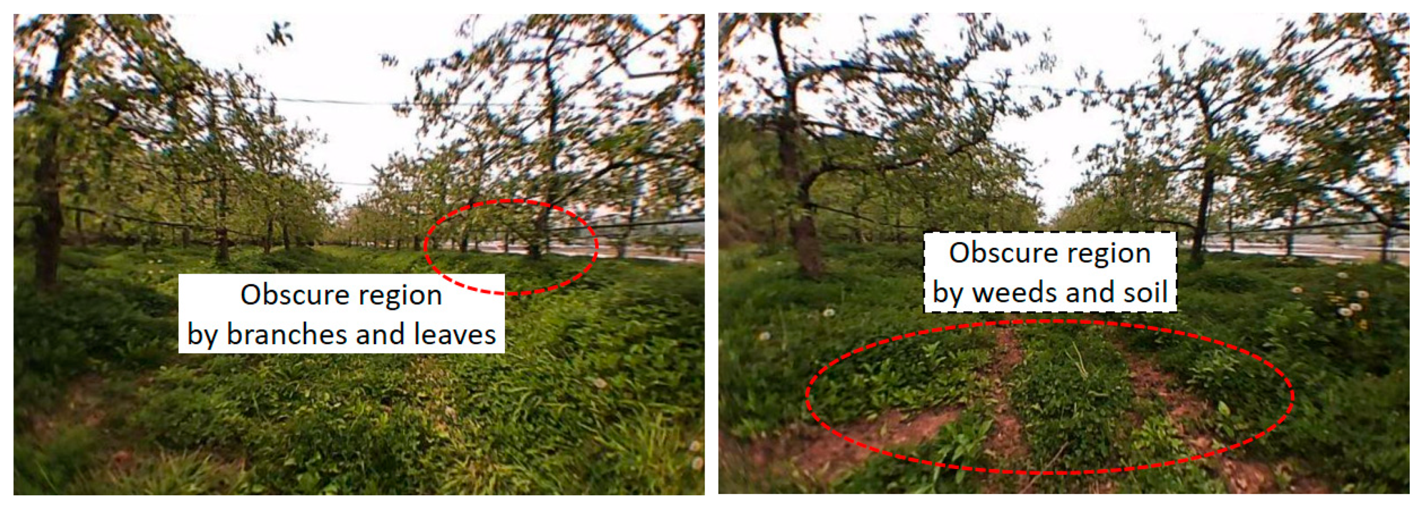
A trunk recognition technique in an orchard environment is a very important technology for precision agriculture of orchard and autonomous driving and autonomous operation of a mobile robot. In this paper, we have proposed an algorithm to recognize trunks and a method to generate a path that an unmanned ground vehicle (UGV) can travel in an apple orchard. In the case of apple trees, the branches are low, so the length of the trunks is short, and the branches and leaves often visually obscure the trunk, as shown in the Figure 1. In addition, the orchard weeds cover the trunk-to-ground boundary, and the ground is irregularly composed of soils and weeds, often making the bottom pattern uneven. For this reason, it becomes more difficult to determine the travelable route based on tree trunks using machine vision.
To detect the trunk’s lowest points, we have applied a naïve Bayesian classification, and extracted free spaces by connecting these points and the center line is generated. For the detection of the trunk, monocular near-infrared (NIR) camera images were converted to a binary image divided into a brightness region containing tree trunks and another region. The lowest points of the segments containing the tree trunks were detected and the tree trunk’s lowest points were determined by applying a naïve Bayesian probabilities. The detected trunk’s lowest points were used to estimate the free space center line of the orchard alley using linear regression analysis, and the alley center line can be used as a movement path or navigation information for the UGV.
2. Apple Orchard Environment and Monocular NIR Camera Condition
2.1. Semi-Structured Apple Orchard Environments
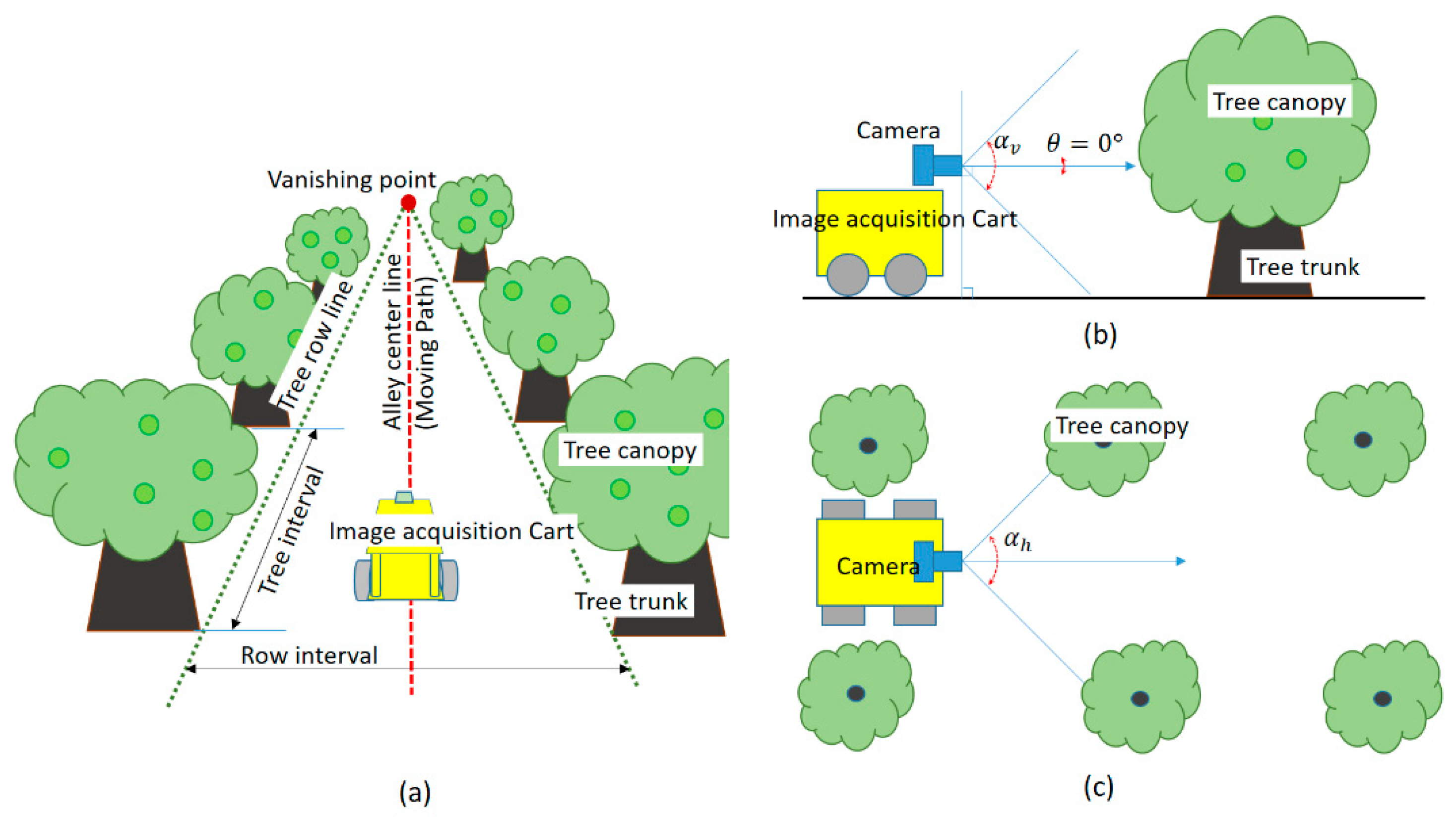
The semi-structured apple orchard, which is the subject of this study, is shown in Figure 1 and Figure 2. It is a typical outdoor natural apple orchard environment, but a bad condition for a self-drive farming machine. The trees are planted in straight row line at intervals of about 1–4 m and the distance between two straight row lines is about 4–8 m. However, even within the same orchard, the interval of the trees and the interval of the rows are not uniform, but varies by several tens of centimeters. The trunks of the trees are also covered sometimes with a lot of weeds, and sometimes they are covered with drooping branches and leaves, as shown in Figure 1. The orchard ground has various different patterns in the areas where the weeds grow and the areas where the soil is revealed. These conditions, which are mentioned above, make it difficult to estimate, based on the image, the navigation path for a self-driving farming machine using a machine vision (MV) method.
2.2. Mono NIR Camera Conditions
As shown in Figure 2, typically, autonomous navigation equipment, such as the information acquisition vehicle for SLAM or image acquisition, the cart must move between two rows of trees in a real orchard.
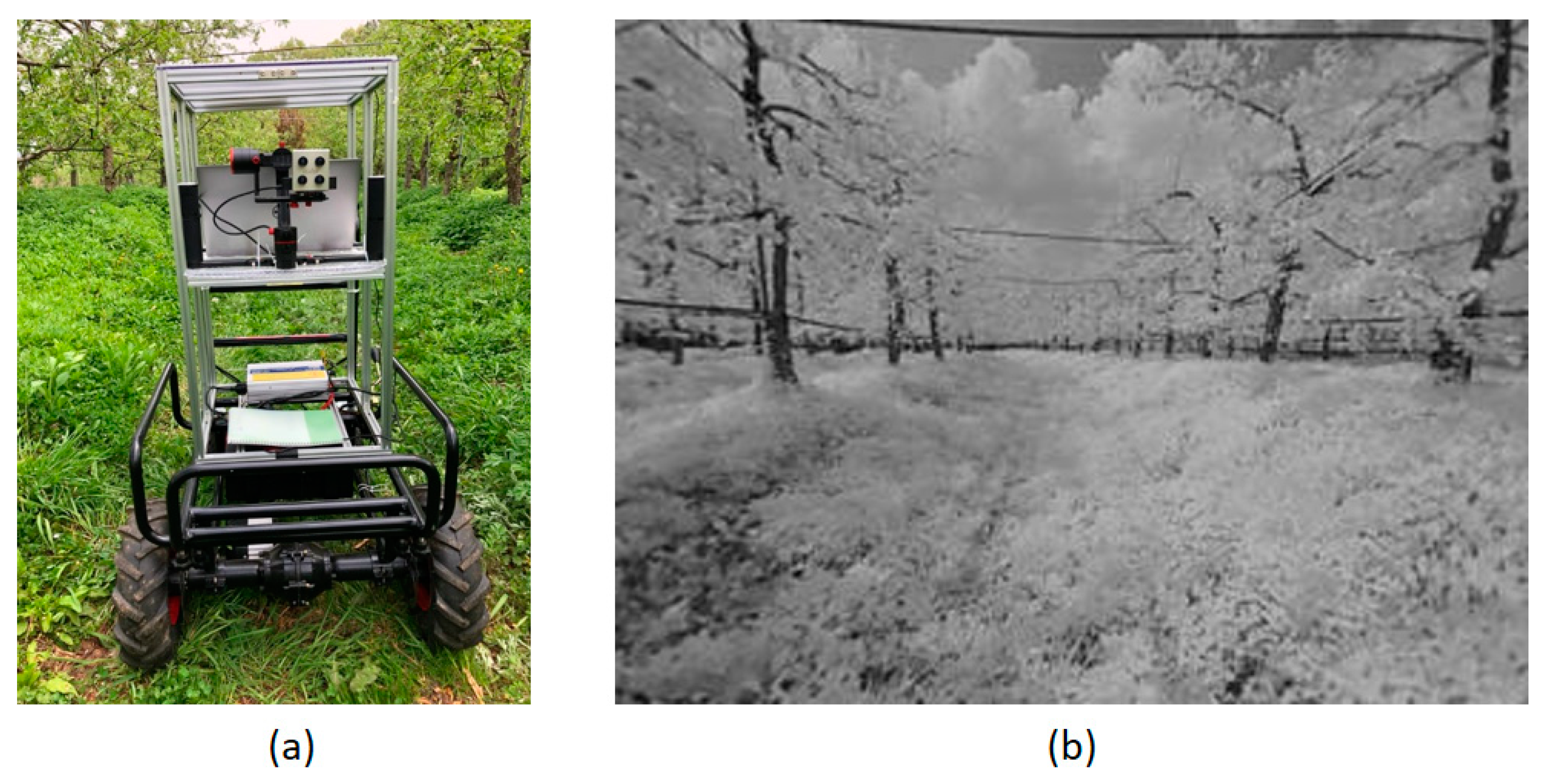
To acquire NIR images of an apple orchard environment, a lab-made image acquisition cart system was developed as shown in Figure 2 and Figure 3a with a CMOS image sensor (CIS) camera. The cart length and width are 1.0 m and 0.8 m, respectively, and Red, Green and Blue (RGB) images and multi-wave band NIR images can be collected using a visible-wavelength camera and three-types of NIR camera. The cart also consists of a power supply, a motor drive unit, a lab-made multi-wave camera, a gimbal for controlling the camera angle, and a computer for the image capture program. The image capture program was developed using LabVIEW. A captured NIR image is shown in Figure 3b. The characteristic of the NIR image in the orchard environment is that the leaves, weeds, cloud, and sky look bright. On the other hand, tree trunks, branches, and soils are relatively dark. The NIR camera used for this experiment is a ≈750–850 nm pass NIR filter. When using NIR active light at ≈750–850 nm, we could estimate free space at night using the proposed algorithm. The camera tilt angle (θ) and roll angle were always set to “zero degree” by using gimbals so that the optical axis of the camera was always parallel to the ground surface of the apple orchard. The horizontal angle () range of the camera was 110 degrees, the vertical angle () range was 100 degrees, and the image resolution was 320 × 240. The camera was installed at a height of 1 m from the surface. For this experiment, we assumed that the speed of the autonomous moving equipment for agricultural work in the orchard was 3.6 km/h. Image acquisition was performed at 25 cm intervals. Under a 3.6 km/h speed condition, image acquisition at 25 cm interval means 4 frame per second. Furthermore, we expect to be able to process four 320 × 240 gray scale images per second, not just at high-performance, but also low-end computer processes. Agricultural autonomous equipment traveling at a speed of 3.6 km/h could be stopped immediately if it should suddenly be in an unexpected situation. Updating and confirming the situation every 25 cm was sufficient for autonomous agriculture operations of agricultural autonomous equipment, detection of obstacles, and securing of travel routes.
3. Naive Bayesian Classification and Navigation Path Estimation
3.1. Gaussian Normal Distribution Likelihood Model
Naïve Bayes classification is a kind of probabilistic classifier applying the Bayesian theorem that assumes that there is mutual independence between class properties, and has been extensively studied in the field of machine learning since the 1950s [19]. In the field of statistics and computer science, the naïve Bayes classifier is being used for text classification and is being used as a popular method for judging a document as one of several categories such as spam, sport, or politics. Despite its naïve design and simplified assumptions, naïve Bayes classifiers are known to work fairly well in many complex real-world situations. In the supervised learning setting, naïve Bayes only needs a small number of training data to determine the parameters needed for classification or to estimate the parameters. In many practical applications, the parameter estimation of the naïve Bayes model uses maximum likelihood estimation (MLE), which is applicable to non-specialists without Bayesian probability or Bayesian methods. The basic assumption of a naïve Bayesian classification is that attribute values within each class will represent a Gaussian distribution. That is, the properties of each class can be represented by property values, such as mean and standard deviation, and the probability of observations can be calculated efficiently using these Gaussian normal distributions. It is known that the Gaussian normal distribution likelihood model can be used among the naïve Bayes classification models, especially if the sample data are all real numbers and the data of the class exhibits a normal distribution. The naïve Bayesian model can be expressed as a probability density function expression for the normal (or Gaussian) distribution as follows [20]:
where, C denotes the class of an instance, x represents a particular observed attribute value, is the average of the values associated with class C, and represents the variance.
3.2. Training a Naïve Bayesian Classifier
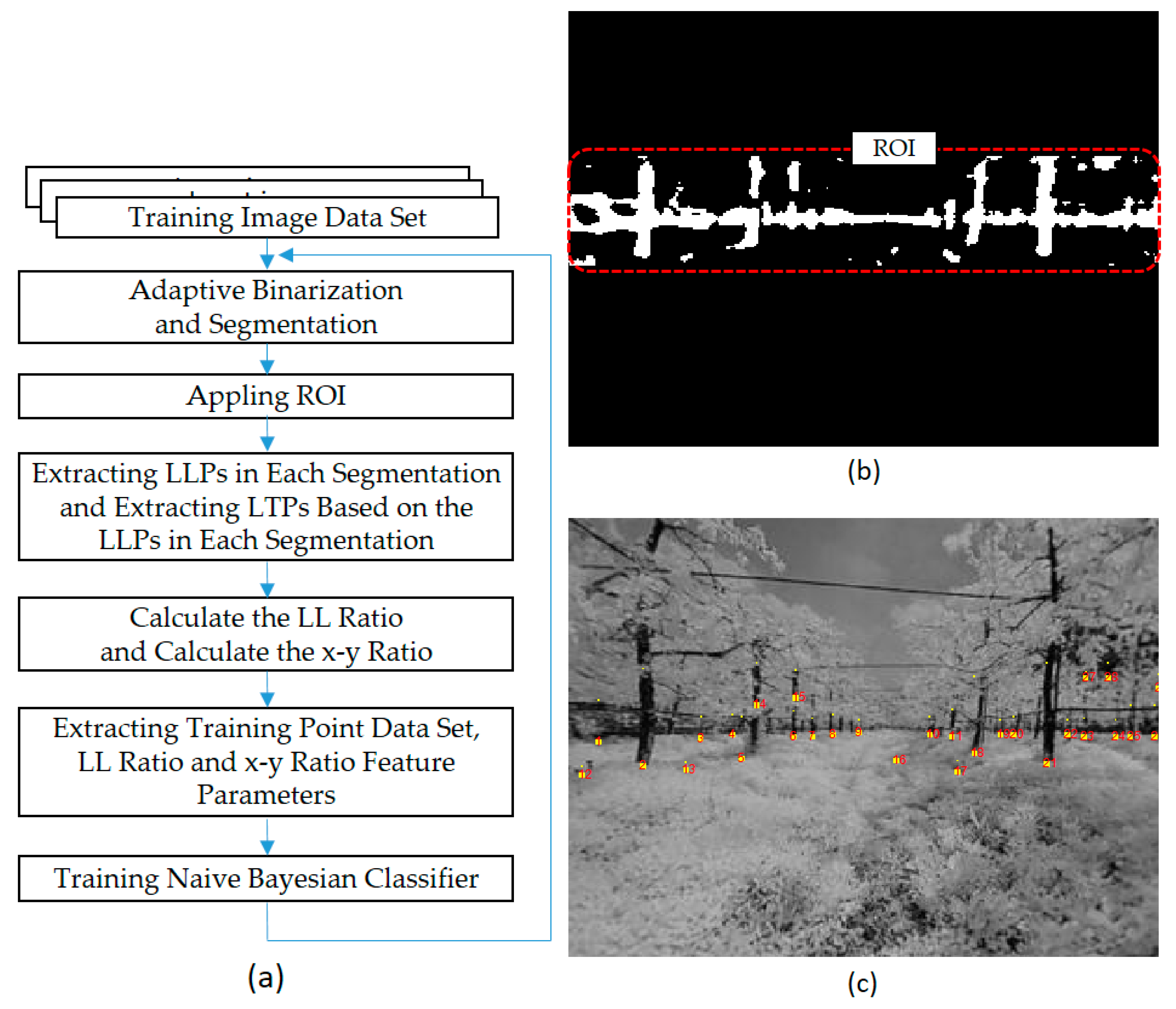
In this paper, we try to detect the alley center line to generate the traveling path of the autonomous working equipment for the orchard. To do this, the trunk’s lowest points should be detected, and the rows of the trees must be detected by connecting these points, and then the alley center line must be calculated in order. The most important and difficult step in this process is to detect the trunk’s lowest points. Naïve Bayesian probabilities are applied to the detection step of the trunk’s lowest points among the alley center line detection algorithms proposed in this paper. To apply naïve Bayesian classification, it is needed to train the naïve Bayesian classifier. The training procedures are explained in Figure 4a. Morphological image preprocessing including blurring, corroding, and dilating corresponding to basic image preprocessing methods was performed on orchard images and converted into binary images.
As shown in Figure 4b, in the binary image, the white area including the tree trunk and the black area including the weeds, the leaves, and the sky are visually distinguishable. However, it contains a lot of noise. As a first step, we extracted the local segment’s lowest points as shown in Figure 4c using the converted binary images. The extracted points were converted into (local lowest) LL ratio and x-y ratio values, and training was performed to complete the naïve Bayesian classifier. The LL ratio is defined as the ratio of the y-value of the LLP (local lowest point) to the distance value between the LTP (local top point) points. Here, LLP is defined as the local lowest boundary point between the white segment and the black background, and LTP is defined as the farthest point located above LLP on the same segment area. The x-y ratio is defined as the ratio of the x-value to the y-value of the LLP point. The data set for training was taken from the apple orchard, and all 36 images were used. The number of data set points (segment’s lowest points) extracted from the binary image was 690 pointers including 246 trunk points and 444 non-trunk points. Once the tilt and roll angles of the camera were set as described in the previous section, the position of the missing line was fixed in the image. Therefore, in this experiment, we set the region of interest (ROI) for the main tree trunk area below the missing line, which was the area where the tree trunk exists, and proceeded with the remaining steps for ROI.
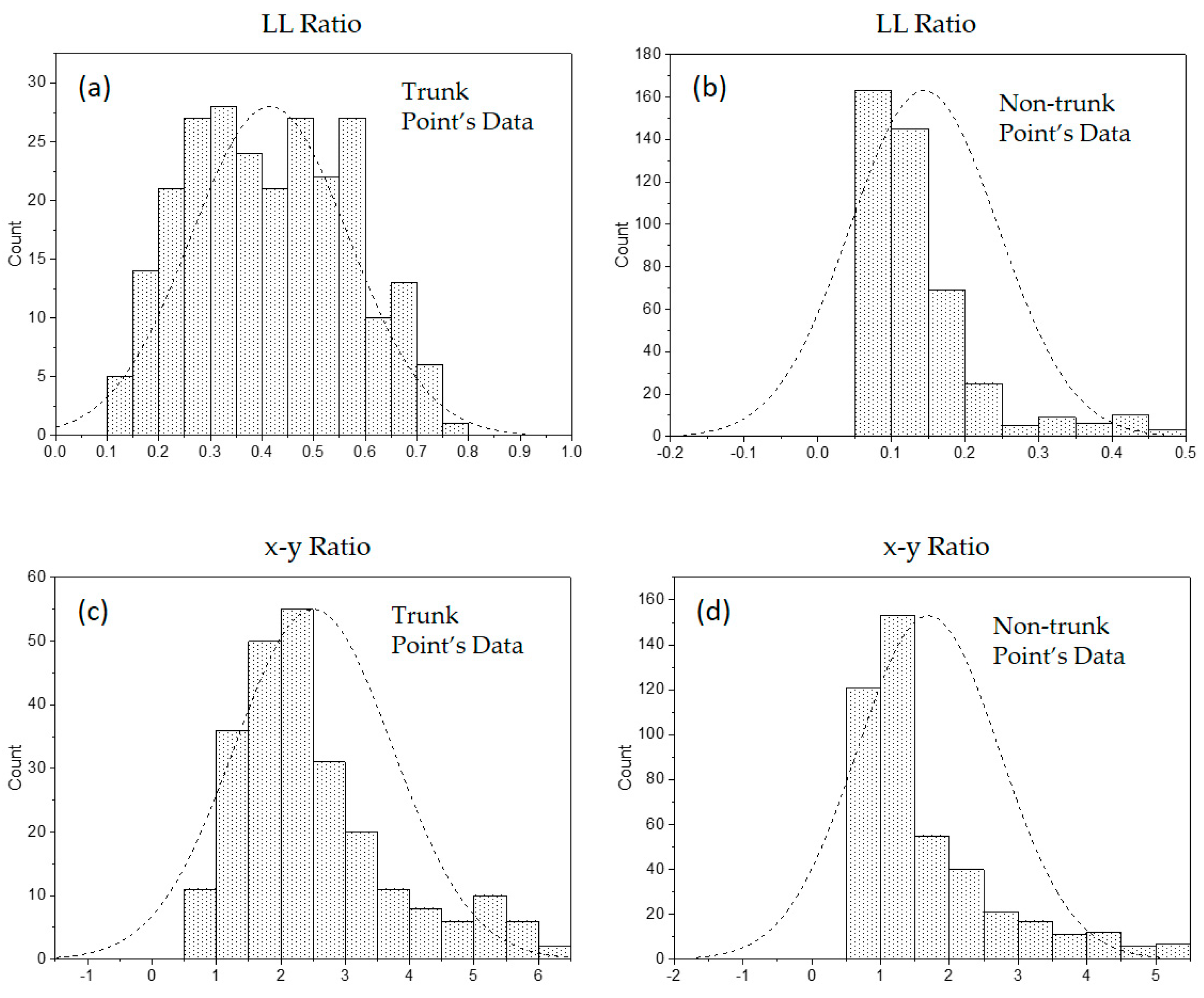
The general assumption for applying a Naive Bayesian classifier is that the distribution of the sample values representing the properties of each class should represent a Gaussian distribution. Therefore, the LL ratio and x-y ratio must be Gaussian distributed to classify them using a naïve Bayesian classification. The distribution of 690 training data set points extracted above is shown in Figure 5, and the four graphs show the Gaussian distribution for this data set for each class. Figure 5a,b shows the distribution of the LL ratio values for the trunk point and the other noise points, respectively. In the same way, Figure 5c,d shows the distribution of the x-y ratio values for the trunk point and the other noise points, respectively. Figure 5a,c shows a symmetrical Gaussian distribution, while Figure 5b,d shows asymmetric characteristics. However, in this study, we modeled the Gaussian distribution with some errors, considering that the data distribution characteristic of the right side near to the trunk point’s data to be compared is a Gaussian distribution form. In general, a Gaussian distribution is shown for each class, so we decided to apply a naïve Bayesian classification.
The mean and variance for each class are summarized in Table 1. The average value of LL ratio for the trunk points was 0.415, the variance was 0.023, the mean value for the x-y ratio was 2.505, and the variance was 1.49. On the other hand, the mean value of the LL ratio for the non-trunk points was 0.144, the variance was 0.011, the mean value for the x-y ratio was 1.64, and the variance was 0.896. These results were used as the properties of the naïve Bayesian classifier for extracting each trunk’s lowest points in this experiment.
3.3. Tree Trunk Lowest Points Extraction and Alley Center Estimation Using Sequence Images
Now we are ready to detect the trunks’ lowest points. This section describes the process of detecting the trunks’ lowest points using the naïve Bayesian classifier. Equation (1) is a model for finding the posterior probabilities for one class of characteristics of each class (e.g., trunk points and non-trunk points). However, in this experiment, two types of class, LL ratio and x-y ratio were applied to improve the accuracy of the estimation result. If the problem instances to be classified are x1 and x2, and these two instance features are independent of each other, the posterior probability of assigning a class variable C to this instance can be expressed as [21]:
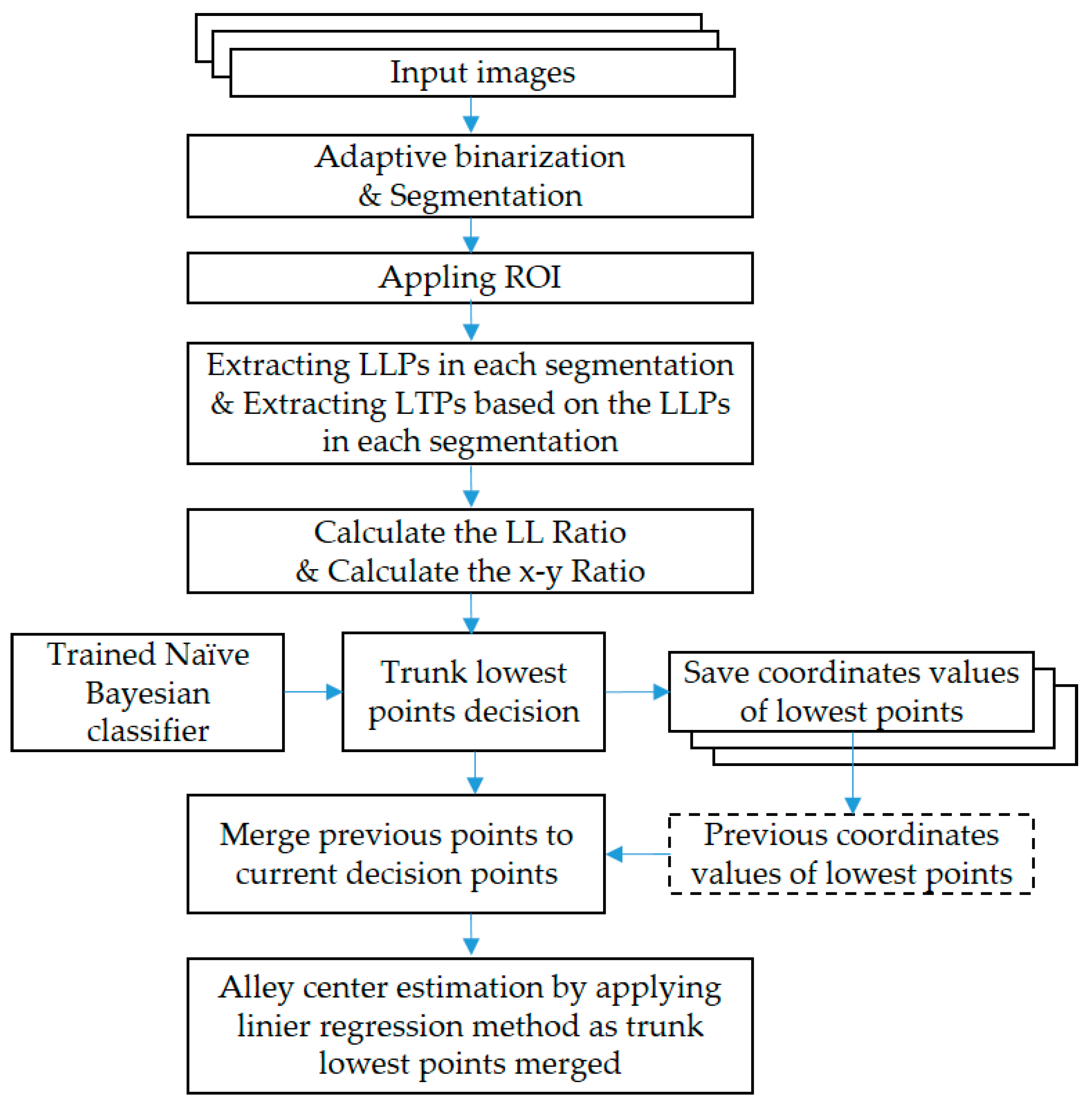
In this study, we want to classify classes corresponding to trunk points and other noise classes. The process block diagram of detecting the lowest points of the trunk using the naïve Bayesian classifier is shown in Figure 6. In order to detect the trunks’ lowest points, morphological image preprocessing including blurring, corroding, and dilating was performed on the input image of the apple orchard similar to the training classifier process and converted into binary images. Next, the LL ratio and x-y ratio were obtained in the area within the main tree trunk area ROI. In Equation (2), instances x1 and x2 that require classification are the LL ratio and x-y ratio, respectively. In addition, the trunks’ points and non-trunks’ points correspond to each class. There are a number of LLP points in the images that were subjected to morphological image preprocessing. Each LLP point could be classified into the trunk’s point class or non-trunk’s point class. In this study, we used Equation (2) to calculate the probability that each LLP point would be classified as a trunk’s point class or as a non-trunk’s point class, and compared the probabilities to the final classification as a larger probability class.
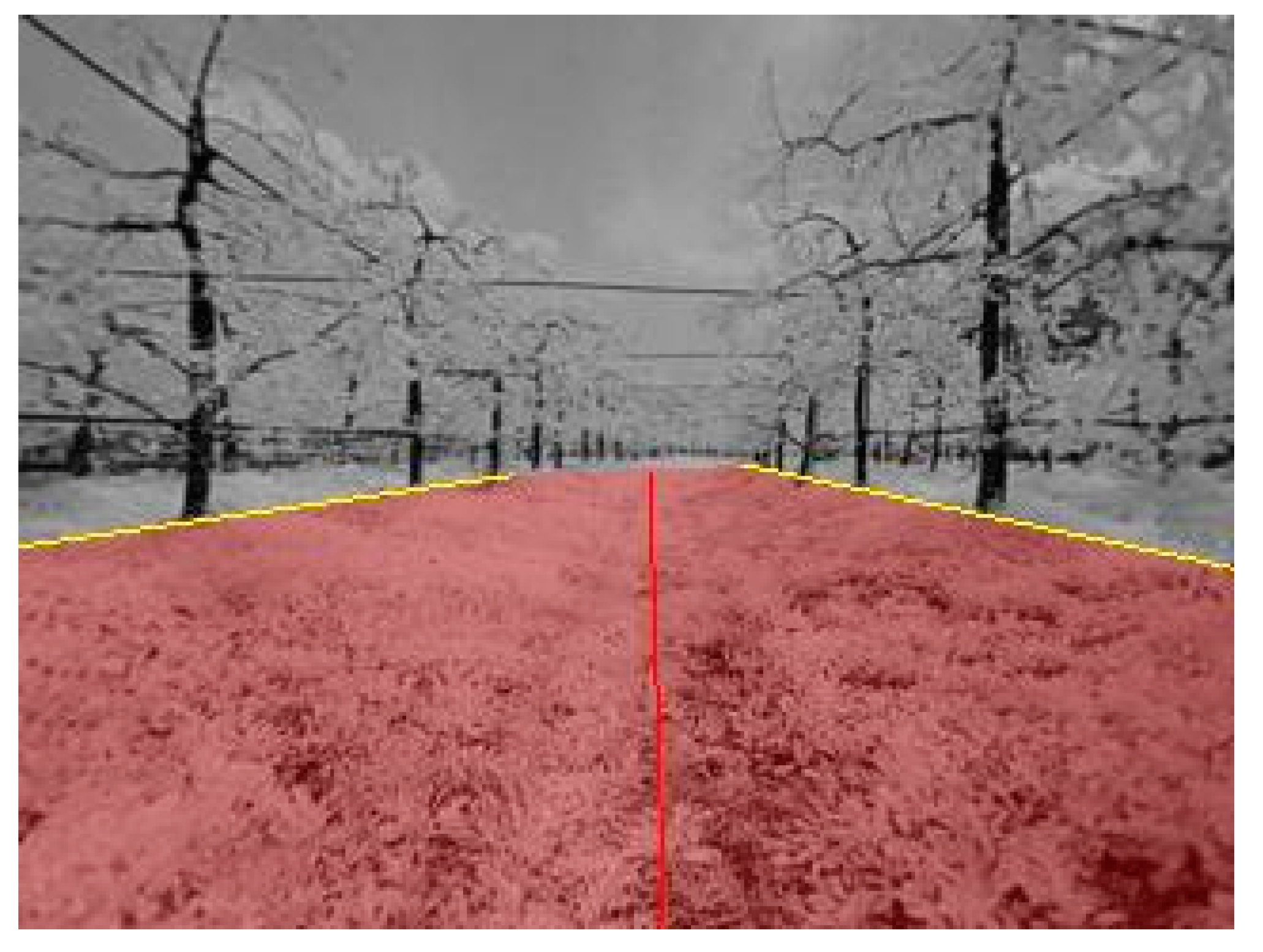
To estimate the center line of the alley, when the classification of the trunk class and the non-trunk class that targets all the LLP points of the image were completed, the linear regression line was calculated using the least squares method for the points classified as the trunk class. For a typical orchard environment, we could get two boundary lines of the orchard alley on the left and right, respectively. The two boundary lines are shown in Figure 7 as two yellow lines. Finally, we calculated the orchard alley center line using these two boundaries and denoted the alley center with a red line in Figure 7. In this experiment, we performed an orchard center line detection experiment on 229 photographs, including 36 images used in naïve Bayesian classifier training.
4. Results and Discussion
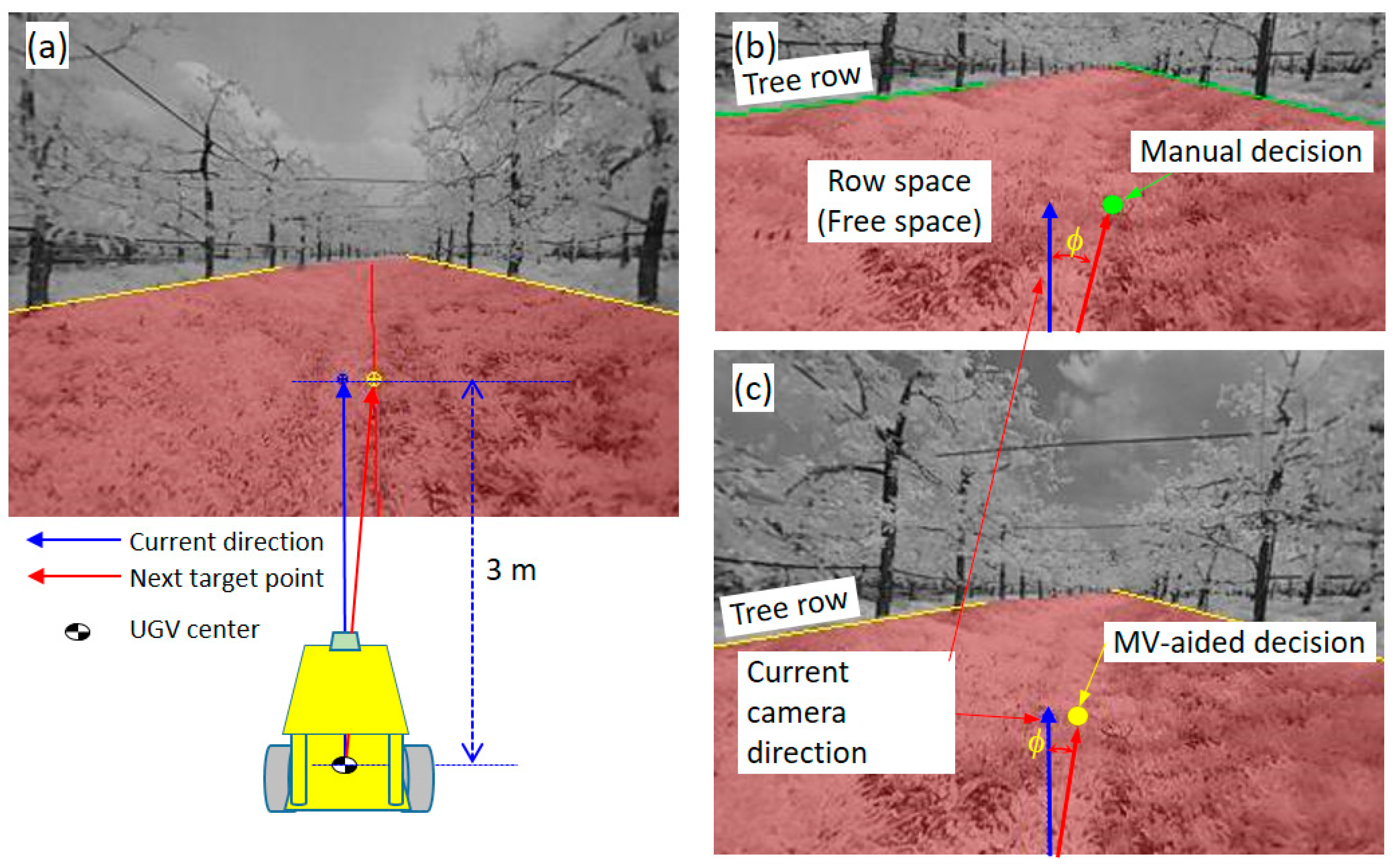
The simplest way to move the unmanned ground vehicle (UGV) is through the steering control from the current reference point to the next point of interest as a method for performing autonomous self-driving. For this operation, it is important to understand the parameter expressing the positional relationship between the current position and the target position. One point on the center line detected through the proposed algorithm is the target point for the next time point for UGV travel. The variables related to the current position of the UGV and the target point could be used as processor variables of the UGV controller. Therefore, in this study, we have calculated the alley center line that represents the center of the free row-space, which was the next target point. After that, the target point and the target steering angle, which were located 3 m ahead the alley center line, were calculated through post-processing. In order to determine the position within the image 3 m ahead, we performed a grid image experiment as shown in Figure 8. As described above, the camera tilt angle (θ) and the roll angle were fixed at 0° so that the optical axis of the camera was always parallel to the ground. The specific y-axis position of the acquired image in this condition corresponded to the specific distance in front. The exact position could be determined through conversion to the bird’s-eye image, but we allowed for some error to minimize the complexity of the algorithm. As shown in Figure 9a–c, the target steering angle, φ, refers to the steering angle to move to the next point 3 m ahead based on current point of the UGV. The manual decision point and the MV-aided decision point also refer to a point 3 m ahead on each line. The total apple orchard continuous images used in this study were collected at intervals of 0.25 m, and 229 images were collected, which corresponded to a 57.25 m alley path. We have evaluated the MV-aided center line extracted by the proposed algorithm by comparing it to the manual center line decided by using the unaided-eye.
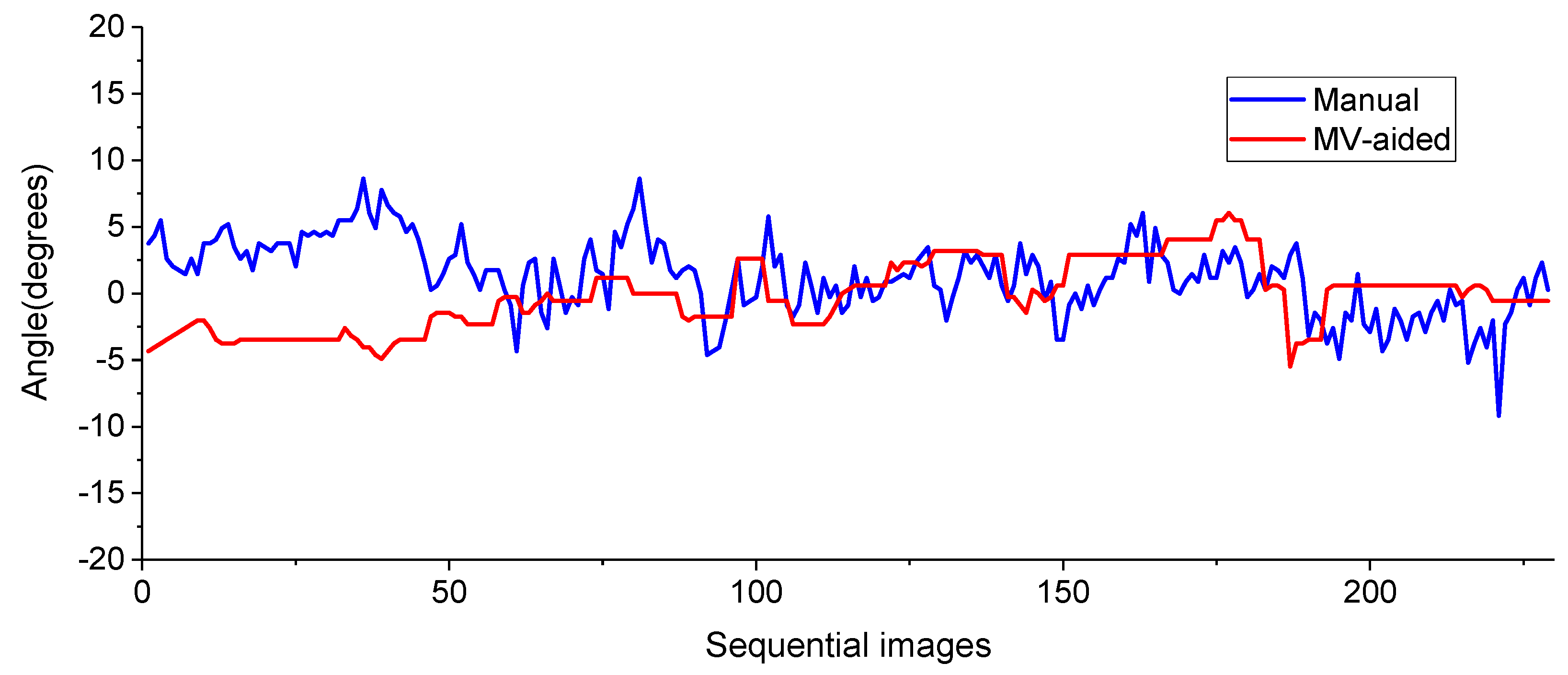
In order to quantitatively compare the characteristics of the manual decision center line and the MV-aided decision center line, we calculated each steering angle based on a point located 3 m ahead of each center line. When the target point was located on the left side based on the current camera direction line, it was expressed as a negative steering angle value, and on the right side, it was expressed as a positive value. The results for 229 images are shown in Figure 10. Through the graph, we can compare the variation of the target steering angles while moving about 57 m, based on the points on the manual center line and MV-aided center line. It can be seen that the change of the steering angle based on the MV-aided center line required more monotonous and relatively stable steering variation than the change based on manual center line.
The average of the 229 steering angles, the maximum left, the maximum right, the standard deviation, and the number of zero crossings were extracted and are shown in Table 2. The mean values of the MV-aided center line and manual center line were −0.2 degrees and 1.3 degrees, respectively. The difference between the mean value of the results of the proposed algorithm and the results of the manual method by visual inspection was about 1.1 degrees. First, for the number of zero crossings, the MV-aided center line and manual center line values were 50 and 27, respectively. The number of zero crossings in this experiment meant the number of times that the zigzag steering was required to match the target position 3 m ahead of the camera center while the UGV travelled about 57 m. Therefore, the larger the number of zero crossing value was, the more the zigzag steering travel of the UGV was, which meant that the driving was unstable. Therefore, it could be concluded that the algorithm proposed in this study was more stable than the unaided-eye manual decision result through the comparison of the number of zero crossings. The maximum left and maximum right values represented the largest left or largest right steering angle among the 229 steering angles calculated to drive to the target point ahead. In the case of maximum left, the values of the MV-aided center line and manual center line were −5.5 degrees and −9.2 degrees, respectively. For the maximum right, the MV-aided center line and manual center line were 6.1 degrees and 8.6 degrees, respectively. In both cases, the results of the algorithm proposed in this study showed a smaller steering angle than the manual decision results. As the result of the comparison of the number of zero crossings, it can be concluded that the proposed algorithm was more stable than the manual center line decision. Finally, the standard deviations of the steer angles obtained from the 229 test images were compared. The standard deviation is a measure of the scattering of the data, defined as the square root of the amount of variance. The smaller the standard deviation, the closer the distance of the variables from the mean value.
As a result of this comparison, the standard deviations shown in Table 2 represent the square root of the difference of the distance between the 229 points in the average value of 229 points extracted from the 229 sample images used in this experiment. As seen in Table 2, the result for the standard deviation of the proposed algorithm was smaller than the manual center line decision. The comparison of the standard deviation shows that the movement path information extracted by the proposed algorithm was more stable than the unaided-eye manual decision center line. As shown in Table 2, the results of the comparison of maximum left, maximum right, standard deviation, and number of zero crossings show that the MV-aided center line calculated from the proposed algorithm was more stable in all items than the manual center line results. The orchard free space and driving center line decision algorithm using the proposed monocular NIR camera for orchard navigation has shown the possibility of guiding a UGV in an apple orchard environment including the noisy environment of apple orchard due to fallen branches, leaves, and a mixed ground pattern with weed and soil areas.
However, in order to use the algorithm proposed in this study, several preconditions were required. First, the camera tilt angle and roll angle were always set to “0” by using gimbals or similar things with the same function so that the optical axis of the camera was always parallel to the ground surface. Second, if the center line was not detected due to various orchard environment changes while driving in the free row space, it was necessary to utilize feedback information such as vehicle posture, speed, and steering angle of the UGV. Third, the orchard environment images used in this experiment may be limited to the case of Fuji varieties of apple trees in the Republic of Korea. Also, even in the same varieties, the orchard environment can be changed according to the cultivation technique and with the seasons. It is necessary to supplement the algorithm through additional experiments in various environments. The algorithm proposed in this study is more effective in the seasons with few leaves on the tree, but in the case of the leafy summer, the image processing method may be different, even if it is an apple orchard of the same region and same variety. In this case, it is necessary to implement an adaptive image processing method such as the sky-based machine vision technique. Another limitation of the proposed approach is that the UGV handles the movement along the central path between trees, but not the end of the line. The end of a tree row can be handled in several ways. One can detect in the image that there were no consecutive tree trunks on the extension of the tree row. Also, ultrasonic sensors can be used to recognize the end of a tree row. In the case of the ≈750–850 nm NIR image used in this study, it is expected that the active light of the corresponding wavelength can be used to acquire images at night, and the proposed algorithm can be used as it is.
5. Conclusions
We have developed an algorithm for the autonomous orchard navigation of a UGV and compared the performance with manually unaided eye-decision results. For this experiment, a monocular NIR CIS camera was used to obtain sample orchard images. The images were converted to a binary image divided into a brightness region containing tree trunks and another region. The lowest points of the segments containing the tree trunks were detected and the tree trunks’ lowest points were determined using a naïve Bayesian classifier. Because the naïve Bayesian classification applied in this study required a small number of samples for training and a simple training process, it was able to effectively classify tree trunks’ points and noise points of the orchard, which were problematic in vision-based processing, and noise caused by small branches, soil, weeds, and tree shadows on the ground. From the classified tree trunks’ points, the trunk row lines were calculated using a linear regression analysis, and the center line of the alley was calculated on two trunk row lines situated on both sides. The performance of the proposed algorithm was investigated using 229 sample images obtained from an image acquisition system. For the performance test, the stabilities of the two center lines extracted by the manual decision and by the MV-aided results using the proposed algorithm were compared and analyzed for the maximum left, the maximum right, the standard deviation, and the number of zero crossings. In all these parameters, the MV-aided center line was more stable than the manual center line results. We are expecting that the proposed algorithm had the potential to take charge of the autonomous driving function of various working vehicles in the orchard for precision agriculture. Our future research would include a method of detecting a more reliable center line and travel route information by integrating center line estimation results and driving information such as vehicle posture, speed, and steering angle of UGV, and the method of recognizing the end of a tree row.
Author Contributions
Conceptualization, H.-K.L., J.-H.P. and B.C.; Methodology, J.-H.P. and S.W.K.; Software, H.-K.L. and D.-H.H.; Investigation, H.-K.L. and D.-H.H.; Writing-Review & Editing, H.-K.L. and B.C.
Funding
This research received no external funding.
Acknowledgments
This study was supported by the Basic Research Program (18-NT-01) through the Daegu Gyeongbuk Institute of Science and Technology (DGIST), and funded by the Ministry of Science, ICT, and Future of Planning of Korea.
Conflicts of Interest
The authors declare no conflict of interest.
References
- Anping, P. Notes on new advancements and revelations in the agricultural archaeology of early rice domestication in the Dongting Lake region. Antiquity 1998, 72, 878–885. [Google Scholar] [CrossRef]
- Zhijun, Z. The Middle Yangtze region in China is one place where rice was domesticated: Phytolith evidence from the Diaotonghuan Cave, Northern Jiangxi. Antiquity 1998, 72, 885–897. [Google Scholar] [CrossRef]
- Pardey, P.G.; Chan-Kang, C.; Dehmer, S.P.; Beddow, J.M. Agricultural R&D is on the move. Nat. News 2016, 537, 301–303. [Google Scholar] [CrossRef] [Green Version]
- Janssen, S.J.; Porter, C.H.; Moore, A.D.; Athanasiadis, I.N.; Foster, I.; Jones, J.W.; Antle, J.M. Towards a new generation of agricultural system data, models and knowledge products: Information and communication technology. Agric. Syst. 2017, 155, 200–212. [Google Scholar] [CrossRef] [PubMed]
- Gebbers, R.; Adamchuk, V.I. Precision agriculture and food security. Science 2010, 327, 828–831. [Google Scholar] [CrossRef] [PubMed]
- Gonzalez-de Soto, M.; Emmi, L.; Perez-Ruiz, M.; Aguera, J.; Gonzalez-de-Santos, P. Autonomous systems for precise spraying–Evaluation of a robotised patch sprayer. Biosyst. Eng. 2016, 146, 165–182. [Google Scholar] [CrossRef]
- Oberti, R.; Marchi, M.; Tirelli, P.; Calcante, A.; Iriti, M.; Tona, E.; Hočevar, M.; Baur, J.; Pfaff, J.; Schütz, C.; et al. Selective spraying of grapevines for disease control using a modular agricultural robot. Biosyst. Eng. 2016, 146, 203–215. [Google Scholar] [CrossRef]
- Zarco-Tejada, P.; Hubbard, N.; Loudjani, P. Precision Agriculture: An Opportunity for EU Farmers—Potential Support with the CAP 2014–2020; Joint Research Centre (JRC) of the European Commission: Brussels, Belgium, 2014. [Google Scholar]
- Shalal, N.; Low, T.; McCarthy, C.; Hancock, N. Orchard mapping and mobile robot localisation using on-board camera and laser scanner data fusion–Part A: Tree detection. Comput. Electron. Agric. 2015, 119, 254–266. [Google Scholar] [CrossRef]
- Shalal, N.; Low, T.; McCarthy, C.; Hancock, N. Orchard mapping and mobile robot localisation using on-board camera and laser scanner data fusion–Part B: Mapping and localisation. Comput. Electron. Agric. 2015, 119, 267–278. [Google Scholar] [CrossRef]
- Dissanayake, G.; Williams, S.B.; Durrant-Whyte, H.; Bailey, T. Map management for efficient simultaneous localization and mapping (SLAM). Auton. Robots 2002, 12, 267–286. [Google Scholar] [CrossRef]
- Asmar, D.C.; Zelek, J.S.; Abdallah, S.M. Tree trunks as landmarks for outdoor vision SLAM. In Proceedings of the 2006 Conference on Computer Vision and Pattern Recognition Workshop (CVPRW’06), New York, NY, USA, 17–22 June 2006; p. 196. [Google Scholar] [CrossRef]
- Cheein, F.A.; Steiner, G.; Paina, G.P.; Carelli, R. Optimized EIF-SLAM algorithm for precision agriculture mapping based on stems detection. Comput. Electron. Agric. 2011, 78, 195–207. [Google Scholar] [CrossRef]
- García-Alegre Sánchez, M.C.; Martin, D.; Guinea García-Alegre, D.M.; Guinea Díaz, D. Real-Time fusion of visual images and laser data images for safe navigation in outdoor environments. In Sensor Fusion; Thomas, C., Ed.; InTech: Rijeka, Croatia, 2011; pp. 221–238. ISBN 978-953-307-446-7. [Google Scholar]
- Ali, W.; Georgsson, F.; Hellstrom, T. Visual tree detection for autonomous navigation in forest environment. In Proceedings of the 2008 IEEE Intelligent Vehicles Symposium, Eindhoven, The Netherlands, 4–6 June 2008; pp. 560–565. [Google Scholar] [CrossRef]
- Shalal, N.; Low, T.; McCarthy, C.; Hancock, N. A preliminary evaluation of vision and laser sensing for tree trunk detection and orchard mapping. In Proceedings of the Australasian Conference on Robotics and Automation (ACRA 2013), Sydney, Australia, 2–4 December 2013; Australasian Robotics and Automation Association: Sydney, Australia, 2013; pp. 1–10. Available online: http://www.araa.asn.au/acra/acra2013/papers/pap162s1-file1.pdf (accessed on 21 August 2018).
- He, B.; Liu, G.; Ji, Y.; Si, Y.; Gao, R. Auto recognition of navigation path for harvest robot based on machine vision. In Proceedings of the International Conference on Computer and Computing Technologies in Agriculture, Nanchang, China, 22–25 October 2000; Springer: Berlin, Germany, 2010; pp. 138–148. [Google Scholar] [CrossRef]
- Radcliffe, J.; Cox, J.; Bulanon, D.M. Machine vision for orchard navigation. Comput. Ind. 2018, 98, 165–171. [Google Scholar] [CrossRef]
- Stuart, R.; Norvig, P. Artificial Intelligence: A Modern Approach, 2nd ed.; Prentice Hall: Upper Saddle River, NJ, USA, 2003; ISBN-10: 0137903952. [Google Scholar]
- John, G.H.; Langley, P. Estimating continuous distributions in Bayesian classifiers. In Proceedings of the Eleventh Conference on Uncertainty in Artificial Intelligence, Montreal, QU, Canada, 18–20 August 1995; Morgan Kaufmann Publishers Inc.: Burlington, MA, USA, 1995; pp. 338–345, ISBN 1-55860-385-9. [Google Scholar]
- Murty, M.N.; Devi, V.S. Pattern Recognition: An Algorithmic Approach; Springer Science & Business Media: Berlin, Germany, 2011; ISBN 9780857294951. [Google Scholar]
Figure 1.
Obscure areas where trunks are blocked by branches and leaves.

Figure 2.
Semi-structured apple orchard environment and camera condition: (a) semi-structured orchard environment, (b) tilt angle and vertical view angle of camera, and (c) horizontal angle of camera.
Figure 2.
Semi-structured apple orchard environment and camera condition: (a) semi-structured orchard environment, (b) tilt angle and vertical view angle of camera, and (c) horizontal angle of camera.

Figure 3.
NIR image acquisition: (a) NIR image acquisition cart system and (b) NIR image captured by the cart system.
Figure 3.
NIR image acquisition: (a) NIR image acquisition cart system and (b) NIR image captured by the cart system.

Figure 4.
(a) Block diagram of training naïve Bayesian classifier, (b) a binary images and ROI after image preprocessing, and (c) extracted local lowest points of white segments in ROI area.
Figure 4.
(a) Block diagram of training naïve Bayesian classifier, (b) a binary images and ROI after image preprocessing, and (c) extracted local lowest points of white segments in ROI area.

Figure 5.
Distribution characteristics of 690 training data set points, (a) the distribution of the LL ratio values for the trunk point and (b) the other noise points, (c) the distribution of the x-y ratio values for the trunk point and (d) the other noise points.
Figure 5.
Distribution characteristics of 690 training data set points, (a) the distribution of the LL ratio values for the trunk point and (b) the other noise points, (c) the distribution of the x-y ratio values for the trunk point and (d) the other noise points.

Figure 6.
Proposed working principle block diagram of the alley center estimation system.

Figure 7.
Estimated two boundary yellow lines and alley center red line.

Figure 8.
Grid-pattern image for forward position mapping.

Figure 9.
Comparison of the manual decision and MV-aided decision. (a) Current UGV direction and target direction. (b) Steering angle, φ, by manual decision. (c) Steering angle, φ by MV-aided decision to compare to the manual decision’s angle.
Figure 9.
Comparison of the manual decision and MV-aided decision. (a) Current UGV direction and target direction. (b) Steering angle, φ, by manual decision. (c) Steering angle, φ by MV-aided decision to compare to the manual decision’s angle.

Figure 10.
Steering angle for the next target point.


Table 1.
The mean and variance values of each class for 690 training data set points.
| Training Data Set | LL Ratio | x-y Ratio | ||
|---|---|---|---|---|
| Mean | Variance | Mean | Variance | |
| Trunk | 0.415 | 0.023 | 2.505 | 1.496 |
| Non-trunk | 0.144 | 0.011 | 1.640 | 0.896 |
Table 2.
Characteristics of sequential 229 images.
| Stability Comparson | Mean [Degree] | Max. Left [Degree] | Max. Right [Degree] | Stdard Deviation [Degree] | Z-Crossing [Number of times] |
|---|---|---|---|---|---|
| Manual decision | 1.3 | −9.2 | 8.6 | 2.8 | 50 |
| MV-aided decision | −0.2 | −5.5 | 6.1 | 2.5 | 27 |
© 2018 by the authors. Licensee MDPI, Basel, Switzerland. This article is an open access article distributed under the terms and conditions of the Creative Commons Attribution (CC BY) license (http://creativecommons.org/licenses/by/4.0/).
Share and Cite
MDPI and ACS Style
Lyu, H.-K.; Park, C.-H.; Han, D.-H.; Kwak, S.W.; Choi, B. Orchard Free Space and Center Line Estimation Using Naive Bayesian Classifier for Unmanned Ground Self-Driving Vehicle. Symmetry 2018, 10, 355. https://doi.org/10.3390/sym10090355
AMA Style
Lyu H-K, Park C-H, Han D-H, Kwak SW, Choi B. Orchard Free Space and Center Line Estimation Using Naive Bayesian Classifier for Unmanned Ground Self-Driving Vehicle. Symmetry. 2018; 10(9):355. https://doi.org/10.3390/sym10090355
Chicago/Turabian StyleLyu, Hong-Kun, Chi-Ho Park, Dong-Hee Han, Seong Woo Kwak, and Byeongdae Choi. 2018. "Orchard Free Space and Center Line Estimation Using Naive Bayesian Classifier for Unmanned Ground Self-Driving Vehicle" Symmetry 10, no. 9: 355. https://doi.org/10.3390/sym10090355
Note that from the first issue of 2016, this journal uses article numbers instead of page numbers. See further details here.