Different Forms of Triangular Neutrosophic Numbers, De-Neutrosophication Techniques, and their Applications

Abstract

In this paper, we introduce the concept of neutrosophic number from different viewpoints. We define different types of linear and non-linear generalized triangular neutrosophic numbers which are very important for uncertainty theory. We introduced the de-neutrosophication concept for neutrosophic number for triangular neutrosophic numbers. This concept helps us to convert a neutrosophic number into a crisp number. The concepts are followed by two application, namely in imprecise project evaluation review technique and route selection problem.

1. Introduction

1.1. Theory of Uncertainty and Uncertainty Quantification

Uncertainty theory playsanimportant role in modeling sciences and engineering problems. However, there is a basic question regarding how we can define or use the uncertainty concept in our mathematical modeling. Researchers around the globe defined many approaches to defining them, and give their various recommendations to using uncertainty theory. There are several literaturestudiesthatclassify some basic uncertain parameters. It should be noted that there is no unique reorientation of the uncertain parameter. For the problem’s purpose or decision makers’ choice, it can be varied and presented as a different application. We now, here, give some info about uncertain parameters, and show how they differ from eachother using the concept of uncertainty using some definition, flowcharts, and diagrams. In this paper, we recommend the researcher to take the uncertain parameter as a parametric interval valued neutrosophic number.

Some basic differences between some uncertain parameters:

If we take Interval number [1] then we can see,

• The information belongs to a certain interval
• There is no concept of membership function

If we take Fuzzy number [2,3], then we can see,

• The concept of belongingness of the elements comes
• The use of membership function is present

If we take Intuitionistic fuzzy number [4], then we can see,

• The concept of belongingness and non-belongingness of the elementscomes
• The use of membership and non-membership function is present

If we take Neutrosophic fuzzy number [5], then we can see,

• The concept of truthiness, falsity, and indeterminacy of the elements comes
• The use of membership function for truthiness, falsity, and indeterminacy is present

Please follow the idea given in the flowchart below, as shown in Figure 1:

1.2. Neutrosophic Number

Fuzzy systems (FSs) and Intuitionistic fuzzy systems (IFSs) cannot successfully deal with a situation where the conclusion is adequate, unacceptable, and decision-maker declaration is uncertain. Therefore, some novel theories are mandatory for solving the problem with uncertainty. The neutrosophic sets (NSs) [5] reflect on the truth membership, indeterminacy membership, and falsity membership concurrently, which is more practical and adequate than FSs and IFSs in commerce, which areuncertain, incomplete, and inconsistent in sequence. Single-valued neutrosophic sets are an extension of NSs which were introduced by Wang et al. [6]. Ye [7] introduced simplify neutrosophic sets, and Peng et al. [8,9] definite their novel operations and aggregation operators. Finally, there are different extensions of NSs, such as interval neutrosophic set [10], bipolar neutrosophic sets [11], and multi-valued neutrosophic sets [12,13]. The decision-making problem [14,15,16,17,18,19,20,21,22,23,24,25,26,27,28,29,30,31,32,33,34,35,36,37,38] is very important in study, when it is with uncertainty.

Although many researchers and scientists have worked in the recently developed neutrosophic method, and applied it in the field of decision making, there is, however, still some viewpoints regarding defining neutrosophic numbers in different forms, and their corresponding de-impreciseness is very important.

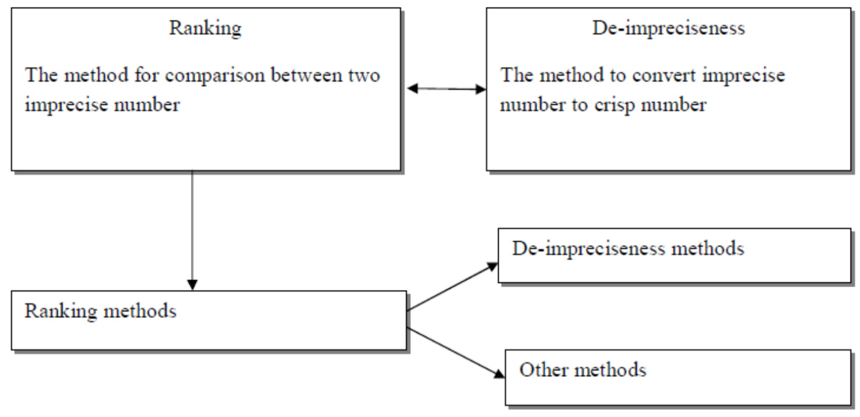
1.3. Ranking and De-Impreciseness

The ranking and de-impreciseness of the imprecise numbers are not a new concept.However, what is the basic concept of the above-said important results and what is the relation. Figure 2 shows the flowchart for de-impreciseness and ranking.

Ranking is a concept where we can compare two imprecise numbers, and de-impreciseness is a technique where the imprecise number is converted to a crisp number. Somewhere, the decision maker takes the two concepts as the same. In this case, they convert the imprecise number into crisp number, and compares them on the basis of crisp value.

1.4. Structure of the Paper

The paper is organized as follows. In Section 1, the basic concept on imprecise set theory and neutrosophic set theory are discussed. Section 2 contains the preliminaries section. Section 3 goes for the known definition of neutrosophic sets and numbers. Single valued linear neutrosophic number and its variation are showing in Section 3. In Section 4, we address the basic concept of neutrosophic non-linear number and generalized neutrosophic number. In Section 5, the de-neutrosophication of linear neutrosophic triangular fuzzy number is performed. The PERT problem is considered in Section 6. The application in assignment problem, considering aproblem, is taken in Section 7. The conclusions are written in Section 8.

2. Neutrosophic Number

Definition 1.

(Neutrosophic Set) A set$\widetilde{S_{neu}}$in the universal discourse$X$, which is denoted generically by$x$, is said to be a neutrosophic set if$\widetilde{S_{neu}}=\{\langle x;[{\pi }_{\widetilde{S_{neu}}}(x),{\mu }_{\widetilde{S_{neu}}}(x),{\vartheta }_{\widetilde{S_{neu}}}(x)]\rangle ⋮x\in X\}$, where${\pi }_{\widetilde{S_{neu}}}(x):X\to \left[0,1\right]$is called the truth membership function which represents the degree of confidence,${\mu }_{\widetilde{S_{neu}}}(x):X\to \left[0,1\right]$is called the indeterminacy membership function which represents the degree of uncertainty, and${\vartheta }_{\widetilde{S_{neu}}}(x):X\to \left[0,1\right]$is called the falsity membership function which represents the degree of scepticism on the decision given the decision maker.

${\pi }_{\widetilde{S_{neu}}}(x),{\mu }_{\widetilde{S_{neu}}}(x)\&{\vartheta }_{\widetilde{S_{neu}}}(x)$ exhibits the following relation:

$$0\le {\pi }_{\widetilde{S_{neu}}}(x)+{\mu }_{\widetilde{S_{neu}}}(x)+{\vartheta }_{\widetilde{S_{neu}}}(x)\le 3$$

Definition 2.

(Single Valued Neutrosophic Set) Neutrosophic set$\widetilde{S_{neu}}$in the definition 2.3, is called a Single Valued Neutrosophic Set$(\widetilde{S_{neu}})$if$x$is a single valued independent variable. Thus$\widetilde{S_{neu}}=\{\langle x;[{\pi }_{\widetilde{S_{neu}}}(x),{\mu }_{\widetilde{S_{neu}}}(x),{\vartheta }_{\widetilde{S_{neu}}}(x)]\rangle ⋮x\in X\}$, where${\pi }_{\widetilde{S_{neu}}}(x),{\mu }_{\widetilde{S_{neu}}}(x)\&{\vartheta }_{\widetilde{S_{neu}}}(x)$represents the truth, indeterminacy, and falsity membership function, respectively, as stated in definition 2.3, and also exhibits the same relationship as stated earlier.

If there exists three points, $a_0,b_0\&c_0$, for which ${\pi }_{\widetilde{S_{neu}}}(a_0)=1,{\mu }_{\widetilde{S_{neu}}}(b_0)=1\&{\vartheta }_{\widetilde{S_{neu}}}(c_0)=1$, then the $\widetilde{S_{neu}}$ is called neut-normal.

A $\widetilde{S_{neu}}$ is said to be neut-convex, which implies that it is a subset of a real line, by satisfying the following conditions:

• ${\pi }_{\widetilde{S_{neu}}}\langle \rho a_1+(1-\rho )a_2\rangle \ge min\langle {\pi }_{\widetilde{S_{neu}}}(a_1),{\pi }_{\widetilde{S_{neu}}}(a_2)\rangle$
• ${\mu }_{\widetilde{S_{neu}}}\langle \rho a_1+(1-\rho )a_2\rangle \le max\langle {\mu }_{\widetilde{S_{neu}}}(a_1),{\mu }_{\widetilde{S_{neu}}}(a_2)\rangle$
• ${\vartheta }_{\widetilde{S_{neu}}}\langle \rho a_1+(1-\rho )a_2\rangle \le max\langle {\vartheta }_{\widetilde{S_{neu}}}(a_1),{\vartheta }_{\widetilde{S_{neu}}}(a_2)\rangle$

where, $a_1\&a_2\in ℝ\mathrm{and}\rho \in \left[0,1\right]$.

Definition 3.

(Single Valued Neutrosophic Number)Single Valued Neutrosophic Number$(\tilde{z})$is defined as$\tilde{z}=\langle [(p^1,q^1,r^1,s^1);\alpha ],[(p^2,q^2,r^2,s^2);\beta ],[(p^3,q^3,r^3,s^3);\gamma ]\rangle$where$\alpha ,\beta ,\gamma \in \left[0,1\right]$, the truth membership function$({\pi }_{\tilde{z}}):ℝ\to \left[0,\alpha \right]$, the indeterminacy membership function$({\mu }_{\tilde{z}}):ℝ\to \left[\beta ,1\right]$, and the falsity membership function$({\vartheta }_{\tilde{z}}):ℝ\to \left[\gamma ,1\right]$is given as:

$$\begin{gathered} {\pi }_{\tilde{z}}(x)=\{\begin{array}{c}{\pi }_{\widetilde{zl}}(x)\\ \alpha \\ \begin{array}{c}{\pi }_{\widetilde{zu}}(x)\\ 0\end{array}\end{array}\begin{array}{c}{p}^1\le x\le q^1\\ q^1\le x\le r^1\\ \begin{array}{c}{r}^1\le x\le s^1\\ \mathrm{otherwise}\end{array}\end{array}, \\ {\mu }_{\tilde{z}}(x)=\{\begin{array}{c}{\mu }_{\widetilde{zl}}(x)\\ \beta \\ \begin{array}{c}{\mu }_{\widetilde{zu}}(x)\\ 1\end{array}\end{array}\begin{array}{c}{p}^2\le x\le q^2\\ q^2\le x\le r^2\\ \begin{array}{c}{r}^2\le x\le s^2\\ \mathrm{otherwise}\end{array}\end{array} \\ {\vartheta }_{\tilde{z}}(x)=\{\begin{array}{c}{\vartheta }_{\widetilde{zl}}(x)\\ \gamma \\ \begin{array}{c}{\vartheta }_{\widetilde{zu}}(x)\\ 1\end{array}\end{array}\begin{array}{c}{p}^3\le x\le q^3\\ q^3\le x\le r^3\\ \begin{array}{c}{r}^3\le x\le s^3\\ \mathrm{otherwise}\end{array}\end{array} \end{gathered}$$

3. Single Valued Linear Neutrosophic Number

• Triangular Single Valued Neutrosophic number of Type 1: The quantity of the truth, indeterminacy and falsity are not dependent: A Triangular Single Valued Neutrosophic number of Type 1 is defined as ${\tilde{\mathrm{A}}}_{\mathrm{Neu}}=({\mathrm{p}}_1,{\mathrm{p}}_2,{\mathrm{p}}_3;{\mathrm{q}}_1,{\mathrm{q}}_2,{\mathrm{q}}_3;{\mathrm{r}}_1,{\mathrm{r}}_2,{\mathrm{r}}_3)$ whose truth membership, indeterminacy and falsity membership is defined as follows:

  $$T_{{\tilde{A}}_{Neu}}(x)=\{\begin{array}{c}\begin{array}{cc}\frac{x-p_1}{p_2-p_1}& \mathrm{when}{p}_1\le x<p_2\end{array}\\ \begin{array}{cc}1& \mathrm{when}x=p_2\end{array}\\ \begin{array}{c}\begin{array}{cc}\frac{p_3-x}{p_3-p_2}& \mathrm{when}{p}_2<x\le p_3\end{array}\\ \begin{array}{cc}0& \mathrm{otherwise}\end{array}\end{array}\end{array}$$

  and

  $$T_{{\tilde{A}}_{Neu}}(x)=\{\begin{array}{c}\begin{array}{cc}\frac{x-p_1}{p_2-p_1}& \mathrm{when}{p}_1\le x<p_2\end{array}\\ \begin{array}{cc}1& \mathrm{when}x=p_2\end{array}\\ \begin{array}{c}\begin{array}{cc}\frac{p_3-x}{p_3-p_2}& \mathrm{when}{p}_2<x\le p_3\end{array}\\ \begin{array}{cc}0& \mathrm{otherwise}\end{array}\end{array}\end{array}$$

  $$I_{{\tilde{A}}_{Neu}}(x)=\{\begin{array}{c}\begin{array}{cc}\frac{q_2-x}{q_2-q_1}& \mathrm{when}{q}_1\le x<q_2\end{array}\\ \begin{array}{cc}0& \mathrm{when}x=q_2\end{array}\\ \begin{array}{c}\begin{array}{cc}\frac{x-q_2}{q_3-q_2}& \mathrm{when}{q}_2<x\le q_3\end{array}\\ \begin{array}{cc}1& \mathrm{otherwise}\end{array}\end{array}\end{array}$$

  and

  $$T_{{\tilde{A}}_{Neu}}(x)=\{\begin{array}{c}\begin{array}{cc}\frac{x-p_1}{p_2-p_1}& \mathrm{when}{p}_1\le x<p_2\end{array}\\ \begin{array}{cc}1& \mathrm{when}x=p_2\end{array}\\ \begin{array}{c}\begin{array}{cc}\frac{p_3-x}{p_3-p_2}& \mathrm{when}{p}_2<x\le p_3\end{array}\\ \begin{array}{cc}0& \mathrm{otherwise}\end{array}\end{array}\end{array}$$

  where, $0\le T_{{\tilde{A}}_{Neu}}(x)+I_{{\tilde{A}}_{Neu}}(x)+F_{{\tilde{A}}_{Neu}}(x)\le 3$, $x\in {\tilde{A}}_{Neu}$.

The parametric form of the above type number is ${({\tilde{A}}_{Neu})}_{\alpha ,\beta ,\gamma }=\left[T_{Neu1}(\alpha ),T_{Neu2}(\alpha );I_{Neu1}(\beta ),I_{Neu2}(\beta );F_{Neu1}(\gamma ),F_{Neu2}(\gamma )\right]$, where,

$$\begin{gathered} T_{Neu1}(\alpha )=p_1+\alpha (p_2-p_1) \\ {T}_{Neu2}(\alpha )=p_3-\alpha (p_3-p_2) \\ {I}_{Neu1}(\beta )=q_2-\beta (q_2-q_1) \\ {I}_{Neu2}(\beta )=q_2+\beta (q_3-q_2) \\ {F}_{Neu1}(\gamma )=r_2-\gamma (r_2-r_1) \\ {F}_{Neu2}(\gamma )=r_2+\gamma (r_3-r_2) \end{gathered}$$

here, $0<\alpha \le 1$, $0<\beta \le 1$, $0<\gamma \le 1$ and $0<\alpha +\beta +\gamma \le 3$

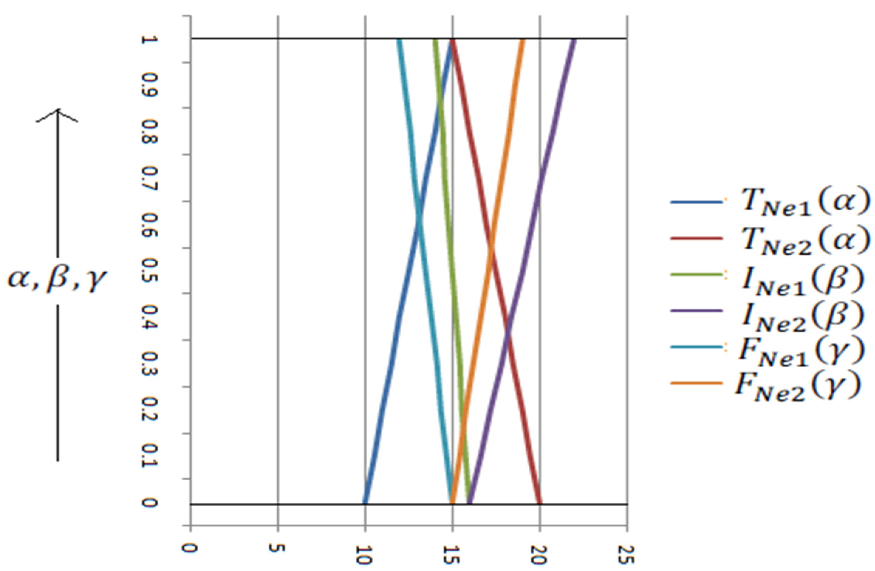
Example 1.

Take${\tilde{A}}_{Ne}=(10,15,20;14,16,22;12,15,19)$.

The parametric representation is

$$\begin{gathered} T_{Ne1}(\alpha )=10+5\alpha \\ {T}_{Ne2}(\alpha )=20-5\alpha \\ {I}_{Ne1}(\beta )=16-2\beta \\ {I}_{Ne1}(\beta )=16+6\beta \\ {F}_{Ne1}(\gamma )=15-3\gamma \\ {F}_{Ne2}(\gamma )=15+4\gamma \end{gathered}$$

Table 1. Value of $T_{Ne1}(\alpha )$, $T_{Ne2}(\alpha )$, $I_{Ne1}(\beta )$, $I_{Ne1}(\beta )$, $F_{Ne1}(\gamma )$, and $F_{Ne2}(\gamma )$.

$\mathit{\alpha }\mathbf{,}\mathit{\beta }\mathbf{,}\mathit{\gamma }$	${\mathit{T}}_{\mathit{N}\mathit{e}\mathbf{1}}\mathbf{\left(}\mathit{\alpha }\mathbf{\right)}$	${\mathit{T}}_{\mathit{N}\mathit{e}\mathbf{2}}\mathbf{\left(}\mathit{\alpha }\mathbf{\right)}$	${\mathit{I}}_{\mathit{N}\mathit{e}\mathbf{1}}\mathbf{\left(}\mathit{\beta }\mathbf{\right)}$	${\mathit{I}}_{\mathit{N}\mathit{e}\mathbf{1}}\mathbf{\left(}\mathit{\beta }\mathbf{\right)}$	${\mathit{F}}_{\mathit{N}\mathit{e}\mathbf{1}}\mathbf{\left(}\mathit{\gamma }\mathbf{\right)}$	${\mathit{F}}_{\mathit{N}\mathit{e}\mathbf{2}}\mathbf{\left(}\mathit{\gamma }\mathbf{\right)}$
0	10	20	16	16	15	15
0.1	10	19.5	15.8	16.6	14.7	15.4
0.2	11	19	15.6	17.2	14.4	15.8
0.3	11.5	18.5	15.4	17.8	14.1	16.2
0.4	12	18	15.2	18.4	13.8	16.6
0.5	12.5	17.5	15	19	13.5	17
0.6	13	17	14.8	19.6	13.2	17.4
0.7	13.5	16.5	14.6	20.2	12.9	17.8
0.8	14	16	14.4	20.8	12.6	18.2
0.9	14.5	15.5	14.2	21.4	12.3	18.6
1	15	15	14	22	12	19

and Figure 3 show the value of $T_{Ne1}(\alpha )$, $T_{Ne2}(\alpha )$, $I_{Ne1}(\beta )$, $I_{Ne1}(\beta )$, $F_{Ne1}(\gamma )$, and $F_{Ne2}(\gamma )$ and graphical representation of triangular single valued neutrosophic numbers (TrSVNNs) respectively.

2.

Triangular Single Valued Neutrosophic Number of Type 2: The quantity of indeterminacy and falsity are dependent: A triangular single valued neutrosophic number (TrSVNN) of Type 2 is defined as ${\tilde{A}}_{Neu}=(p_1,p_2,p_3;q_1,q_2,q_3;u_{Neu},y_{Neu})$ whose truth membership, indeterminacy, and falsity membership are defined as follows:

$$T_{{\tilde{A}}_{Neu}}(x)=\{\begin{array}{c}\begin{array}{cc}\frac{x-p_1}{p_2-p_1}& \mathrm{when}{p}_1\le x<p_2\end{array}\\ \begin{array}{cc}1& \mathrm{when}x=p_2\end{array}\\ \begin{array}{c}\begin{array}{cc}\frac{p_3-x}{p_3-p_2}& \mathrm{when}{p}_2<x\le p_3\end{array}\\ \begin{array}{cc}0& \mathrm{otherwise}\end{array}\end{array}\end{array}$$

and

$$I_{{\tilde{A}}_{Neu}}(x)=\{\begin{array}{c}\begin{array}{cc}\frac{q_2-x+u_{Neu}(x-q_1)}{q_2-q_1}& \mathrm{when}{q}_1\le x<q_2\end{array}\\ \begin{array}{cc}{u}_{Neu}& \mathrm{when}x=q_2\end{array}\\ \begin{array}{c}\begin{array}{cc}\frac{x-q_2+u_{Neu}(q_3-x)}{q_3-q_2}& \mathrm{when}{q}_2<x\le q_3\end{array}\\ \begin{array}{cc}1& \mathrm{otherwise}\end{array}\end{array}\end{array}$$

and

$$F_{{\tilde{A}}_{Neu}}(x)=\{\begin{array}{c}\begin{array}{cc}\frac{q_2-x+y_{Neu}(x-q_1)}{q_2-q_1}& \mathrm{when}{q}_1\le x<q_2\end{array}\\ \begin{array}{cc}{y}_{Neu}& \mathrm{when}x=q_2\end{array}\\ \begin{array}{c}\begin{array}{cc}\frac{x-q_2+y_{Neu}(q_3-x)}{q_3-q_2}& \mathrm{when}{q}_2<x\le q_3\end{array}\\ \begin{array}{cc}1& \mathrm{otherwise}\end{array}\end{array}\end{array}$$

where, $0\le T_{{\tilde{A}}_{Neu}}(x)+I_{{\tilde{A}}_{Neu}}(x)+F_{{\tilde{A}}_{Neu}}(x)\le 2$, $x\in {\tilde{A}}_{Neu}$.

The parametric form of the above type number is ${({\tilde{A}}_{Neu})}_{\alpha ,\beta ,\gamma }=\left[T_{Neu1}(\alpha ),T_{Neu2}(\alpha );I_{Neu1}(\beta ),I_{Neu2}(\beta );F_{Neu1}(\gamma ),F_{Neu2}(\gamma )\right]$, where

$$\begin{gathered} T_{Neu1}(\alpha )=p_1+\alpha (p_2-p_1) \\ {T}_{Neu2}(\alpha )=p_3-\alpha (p_3-p_2) \\ {I}_{Neu1}(\beta )=\frac{q_2-u_{Neu}{q}_1-\beta (q_2-q_1)}{1-u_{Neu}} \\ {I}_{Neu2}(\beta )=\frac{q_2-u_{Neu}{q}_3+\beta (q_3-q_2)}{1-u_{Neu}} \\ {F}_{Neu1}(\gamma )=\frac{q_2-y_{Neu}{q}_1-\gamma (q_2-q_1)}{1-y_{Neu}} \\ {F}_{Neu2}(\gamma )=\frac{q_2-y_{Neu}{q}_3+\gamma (q_3-q_2)}{1-y_{Neu}}. \end{gathered}$$

Here, $0<\alpha \le 1$, $u_{Neu}<\beta \le 1$, $y_{Neu}<\gamma \le 1$ and $0<\beta +\gamma \le 1$ and $0<\alpha +\beta +\gamma \le 2$.

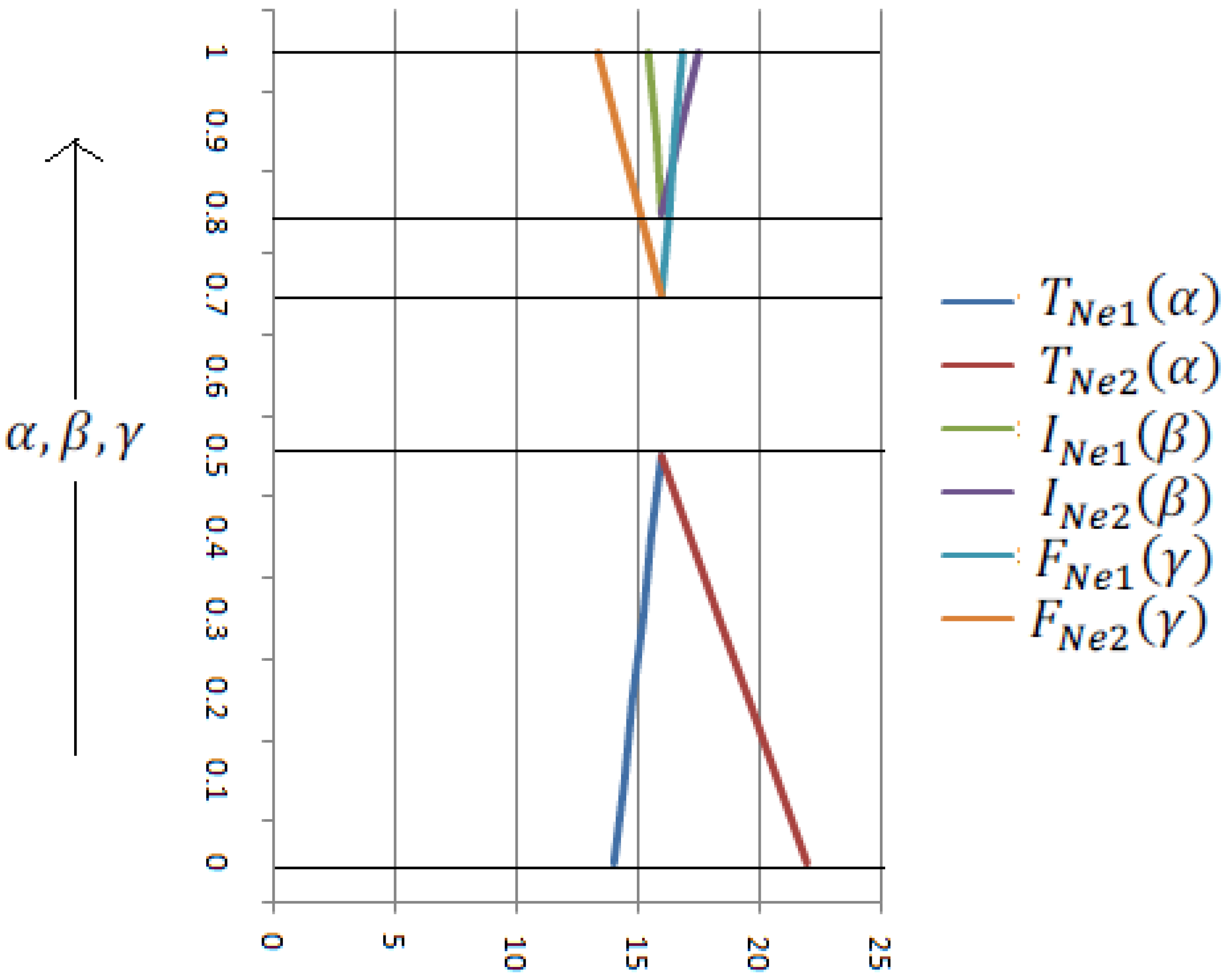
Example 2.

Take${\tilde{A}}_{Ne}=(10,15,20;14,16,22;0.4,0.5)$

The parametric representation is,

$$\begin{gathered} T_{Ne1}(\alpha )=10+5\alpha \\ {T}_{Ne2}(\alpha )=20-5\alpha \\ {I}_{Ne1}(\beta )=\frac{1}{3}(52-10\beta ) \\ {I}_{Ne1}(\beta )=12+10\beta \\ {F}_{Ne1}(\gamma )=18-4\gamma \\ {F}_{Ne2}(\gamma )=10+12\gamma . \end{gathered}$$

Table 2. Value of $T_{Ne1}(\alpha )$, $T_{Ne2}(\alpha )$, $I_{Ne1}(\beta )$, $I_{Ne1}(\beta )$, $F_{Ne1}(\gamma )$, and $F_{Ne2}(\gamma )$.

$\mathit{\alpha }\mathbf{,}\mathit{\beta }\mathbf{,}\mathit{\gamma }$	${\mathit{T}}_{\mathit{N}\mathit{e}\mathbf{1}}\mathbf{\left(}\mathit{\alpha }\mathbf{\right)}$	${\mathit{T}}_{\mathit{N}\mathit{e}\mathbf{2}}\mathbf{\left(}\mathit{\alpha }\mathbf{\right)}$	${\mathit{I}}_{\mathit{N}\mathit{e}\mathbf{1}}\mathbf{\left(}\mathit{\beta }\mathbf{\right)}$	${\mathit{I}}_{\mathit{N}\mathit{e}\mathbf{1}}\mathbf{\left(}\mathit{\beta }\mathbf{\right)}$	${\mathit{F}}_{\mathit{N}\mathit{e}\mathbf{1}}\mathbf{\left(}\mathit{\gamma }\mathbf{\right)}$	${\mathit{F}}_{\mathit{N}\mathit{e}\mathbf{2}}\mathbf{\left(}\mathit{\gamma }\mathbf{\right)}$
0	10	20	–	–	–	–
0.1	10.5	19.5	–	–	–	–
0.2	11	19	–	–	–	–
0.3	11.5	18.5	–	–	–	–
0.4	12	18	16	16	–	–
0.5	12.5	17.5	15.6667	17	16	16
0.6	13	17	15.3333	18	15.6	17.2
0.7	13.5	16.5	15.	19	15.2	18.4
0.8	14	16	14.6667	20	14.8	19.6
0.9	14.5	15.5	14.3333	21	14.4	20.8
1	15	15	14	22	14	22

and Figure 4 show the value of $T_{Ne1}(\alpha )$, $T_{Ne2}(\alpha )$, $I_{Ne1}(\beta )$, $I_{Ne1}(\beta )$, $F_{Ne1}(\gamma )$, and $F_{Ne2}(\gamma )$ and graphical representation of type-2 TrSVNNs.

3.

Triangular Single Valued Neutrosophic number of Type 3: The quantity of the truth, indeterminacy, and falsity are dependent: A TrSVNN of Type 3 is defined as ${\tilde{A}}_{Neu}=(p_1,p_2,p_3;w_{Ne},u_{Neu},y_{Neu})$, whose truth membership, indeterminacy, and falsity membership are defined as follows:

$$T_{{\tilde{A}}_{Neu}}(x)=\{\begin{array}{c}{w}_{Neu}\frac{x-p_1}{p_2-p_1}\mathrm{when}{p}_1\le x<p_2\\ w_{Neu}\mathrm{when}x=p_2\\ \begin{array}{c}{w}_{Neu}\frac{p_3-x}{p_3-p_2}\\ 0\mathrm{otherwise}\end{array}\mathrm{when}{p}_2<x\le p_3\end{array}$$

and

$$I_{{\tilde{A}}_{Neu}}(x)=\{\begin{array}{c}\frac{p_2-x+u_{Neu}(x-p_1)}{p_2-p_1}\mathrm{when}{p}_1\le x<p_2\\ u_{Neu}\mathrm{when}x=p_2\\ \begin{array}{c}\frac{x-p_2+u_{Neu}(p_3-x)}{p_3-p_2}\\ 1\mathrm{otherwise}\end{array}\mathrm{when}{p}_2<x\le p_3\end{array}$$

and

$$I_{{\tilde{A}}_{Neu}}(x)=\{\begin{array}{c}\frac{p_2-x+u_{Neu}(x-p_1)}{p_2-p_1}\mathrm{when}{p}_1\le x<p_2\\ u_{Neu}\mathrm{when}x=p_2\\ \begin{array}{c}\frac{x-p_2+u_{Neu}(p_3-x)}{p_3-p_2}\\ 1\mathrm{otherwise}\end{array}\mathrm{when}{p}_2<x\le p_3\end{array}$$

where, $0\le T_{{\tilde{A}}_{Neu}}(x)+I_{{\tilde{A}}_{Neu}}(x)+F_{{\tilde{A}}_{Neu}}(x)\le 1$, $x\in {\tilde{A}}_{Neu}$.

The parametric form of the above type number is ${({\tilde{A}}_{Neu})}_{\alpha ,\beta ,\gamma }=\left[T_{Neu1}(\alpha ),T_{Neu2}(\alpha );I_{Neu1}(\beta ),I_{Neu2}(\beta );F_{Neu1}(\gamma ),F_{Neu2}(\gamma )\right]$, where

$$\begin{gathered} T_{Neu1}(\alpha )=p_1+\frac{\alpha }{w_{Neu}}(p_2-p_1) \\ {T}_{Neu2}(\alpha )=p_3-\frac{\alpha }{w_{Neu}}(p_3-p_2) \\ {I}_{Neu1}(\beta )=\frac{p_2-u_{Neu}{p}_1-\beta (p_2-p_1)}{1-u_{Neu}} \\ {I}_{Neu2}(\beta )=\frac{p_2-u_{Neu}{p}_3+\beta (p_3-p_2)}{1-u_{Neu}} \\ {F}_{Neu1}(\gamma )=\frac{p_2-y_{Neu}{p}_1-\gamma (p_2-p_1)}{1-y_{Neu}} \\ {F}_{Neu2}(\gamma )=\frac{p_2-y_{Neu}{p}_3+\gamma (p_3-p_2)}{1-y_{Neu}}. \end{gathered}$$

Here, $0<\alpha \le w_{Neu}$, $u_{Neu}<\beta \le 1$, $y_{Neu}<\gamma \le 1$, and $0<\alpha +\beta +\gamma \le 1$.

Example 3.

Take${\tilde{A}}_{Ne}=(14,16,22;0.5,0.8,0.7)$

The parametric representation is,

$$\begin{gathered} T_{Ne1}(\alpha )=14+4\alpha \\ {T}_{Ne2}(\alpha )=22-12\alpha \\ {I}_{Ne1}(\beta )=16-\frac{5}{2}\beta \\ {I}_{Ne1}(\beta )=16+\frac{15}{2}\beta \\ {F}_{Ne1}(\gamma )=16-\frac{20}{7}\gamma \\ {F}_{Ne2}(\gamma )=16+\frac{60}{7}\gamma . \end{gathered}$$

Table 3. Value of $T_{Ne1}(\alpha )$, $T_{Ne2}(\alpha )$, $I_{Ne1}(\beta )$, $I_{Ne1}(\beta )$, $F_{Ne1}(\gamma )$ and $F_{Ne2}(\gamma )$.

$\mathit{\alpha }\mathbf{,}\mathit{\beta }\mathbf{,}\mathit{\gamma }$	${\mathit{T}}_{\mathit{N}\mathit{e}\mathbf{1}}\mathbf{\left(}\mathit{\alpha }\mathbf{\right)}$	${\mathit{T}}_{\mathit{N}\mathit{e}\mathbf{2}}\mathbf{\left(}\mathit{\alpha }\mathbf{\right)}$	${\mathit{I}}_{\mathit{N}\mathit{e}\mathbf{1}}\mathbf{\left(}\mathit{\beta }\mathbf{\right)}$	${\mathit{I}}_{\mathit{N}\mathit{e}\mathbf{1}}\mathbf{\left(}\mathit{\beta }\mathbf{\right)}$	${\mathit{F}}_{\mathit{N}\mathit{e}\mathbf{1}}\mathbf{\left(}\mathit{\gamma }\mathbf{\right)}$	${\mathit{F}}_{\mathit{N}\mathit{e}\mathbf{2}}\mathbf{\left(}\mathit{\gamma }\mathbf{\right)}$
0	14	22
0.1	14.4	20.8
0.2	14.8	19.6
0.3	15.2	18.4
0.4	15.6	17.2
0.5	16	16
0.6
0.7					16	16
0.8			16	16	16.2857	15.1429
0.9			15.75	16.75	16.5714	14.2857
1			15.5	17.5	16.8571	13.4286

and Figure 5 show the value of $T_{Ne1}(\alpha )$, $T_{Ne2}(\alpha )$, $I_{Ne1}(\beta )$, $I_{Ne1}(\beta )$, $F_{Ne1}(\gamma )$ and $F_{Ne2}(\gamma )$. and Graphical representation of type-3 TrSVNNs

Different Operational Laws of Two Triangular Neutrosophic Numbers: If ${\tilde{A}}_{Neu}$ and ${\tilde{B}}_{Neu}$ are two single valued neutrosophic numbers with nine components having truthmembership $T_{{\tilde{A}}_{Neu}}\&T_{{\tilde{B}}_{Neu}}$, indeterminacymembership $I_{{\tilde{A}}_{Neu}}\&I_{{\tilde{B}}_{Neu}}$, and falsitymembership $F_{{\tilde{A}}_{Neu}}\&F_{{\tilde{B}}_{Neu}}$, respectively, such as:

$${\tilde{A}}_{Neu}=\langle a_1,a_2,a_3;b_1,b_2,b_3;c_1,c_2,c_3\rangle \mathrm{and}{\tilde{B}}_{Neu}=\langle a_4,a_5,a_6;b_4,b_5,b_6;c_4,c_5,c_6\rangle$$

where a, band c are the scores given by the decision maker in the scale, ranging from lower limit L_l to upper limit U_l.

• Addition

  $$\begin{array}{l}{\tilde{C}}_{Neu}={\tilde{A}}_{Neu}+{\tilde{B}}_{Neu}\\ =\langle \begin{array}{c}\left\{min(a_1+a_4,U_l),min(a_2+a_5,U_l),min(a_3+raphicalrepresentationoftype3TrSVNNs{a}_6,U_l)\right\};\\ \left\{min(b_1+b_4,U_l),min(b_2+b_5,U_l),min(b_3+b_6,U_l)\right\};\left\{min(c_1+c_4,U_l),min(c_2+c_5,U_l),min(c_3+c_6,U_l)\right\}\end{array}\rangle \end{array}$$
• Negative of SVNNs

  $$\begin{array}{l}{\tilde{S}}_{Neu}=-{\tilde{A}}_{Neu}\\ =\langle -a_3,-a_2,-a_1;-b_3,-b_2,-b_1;-c_3,-c_2,-c_1\rangle \end{array}$$
• Subtraction

  $$\begin{array}{l}{\tilde{D}}_{Neu}={\tilde{A}}_{Neu}-{\tilde{B}}_{Neu}\\ ={\tilde{A}}_{Neu}+(-{\tilde{B}}_{Neu})\\ =\langle \begin{array}{c}\left\{max(a_1-a_6,L_l),max(a_2-a_5,L_l),max(a_3-a_4,L_l)\right\};\\ \left\{max(b_1-b_6,L_l),max(b_2-b_5,L_l),max(b_3-b_4,L_l)\right\};\\ \left\{max(c_1-c_6,L_l),max(c_2-c_5,L_l),max(c_3-c_4,L_l)\right\}\end{array}\rangle \end{array}$$
• Multiplications

  $$\begin{array}{l}{\tilde{D}}_{Neu}={\tilde{A}}_{Neu}-{\tilde{B}}_{Neu}\\ ={\tilde{A}}_{Neu}+(-{\tilde{B}}_{Neu})\\ =\langle \begin{array}{c}\left\{max(a_1-a_6,L_l),max(a_2-a_5,L_l),max(a_3-a_4,L_l)\right\};\\ \left\{max(b_1-b_6,L_l),max(b_2-b_5,L_l),max(b_3-b_4,L_l)\right\};\\ \left\{max(c_1-c_6,L_l),max(c_2-c_5,L_l),max(c_3-c_4,L_l)\right\}\end{array}\rangle \end{array}$$
• Multiplication by a constant

  $$\begin{array}{l}{\tilde{E}}_{Neu}=k\left[{\tilde{A}}_{Neu}\right]\\ =k\times \langle a_1,a_2,a_3;b_1,b_2,b_3;c_1,c_2,c_3\rangle \\ =\langle k{a}_1,k{a}_2,k{a}_3;k{b}_1,k{b}_2,k{b}_3;k{c}_1,k{c}_2,k{c}_3\rangle \end{array}$$
• Inverse of SVNNs

  $$\begin{array}{l}{\tilde{F}}_{Neu}={\tilde{A}}_{Neu}^{-1}=\frac{1}{\langle a_1,a_2,a_3;b_1,b_2,b_3;c_1,c_2,c_3\rangle }\\ =\langle \frac{1}{a_3},\frac{1}{a_2},\frac{1}{a_1};\frac{1}{b_3},\frac{1}{b_2},\frac{1}{b_1};\frac{1}{c_3},\frac{1}{c_2},\frac{1}{c_1}\rangle for(a,b,c)>0\\ =\langle \frac{1}{a_1},\frac{1}{a_2},\frac{1}{a_3};\frac{1}{b_1},\frac{1}{b_2},\frac{1}{b_3};\frac{1}{c_1},\frac{1}{c_2},\frac{1}{c_3}\rangle for(a,b,c)<0\end{array}$$
• Divisions

  $$\begin{array}{l}{\tilde{G}}_{Neu}{\tilde{A}}_{Neu}÷{\tilde{B}}_{Neu}\\ ={\tilde{A}}_{Neu}÷{\tilde{B}}_{Neu}\\ =\langle a_1,a_2,a_3;b_1,b_2,b_3;c_1,c_2,c_3\rangle \times \langle \frac{1}{a_6},\frac{1}{a_5},\frac{1}{a_4};\frac{1}{b_6},\frac{1}{b_5},\frac{1}{b_4};\frac{1}{c_6},\frac{1}{c_5},\frac{1}{c_4}\rangle \\ =\langle \begin{array}{c}\left\{\begin{array}{c}min(\frac{a_1}{a_4},\frac{a_1}{a_5},\frac{a_1}{a_6},\frac{a_2}{a_4},\frac{a_2}{a_5},\frac{a_2}{a_6}=visionofSVNNs,\frac{a_3}{a_4},\frac{a_3}{a_5},\frac{a_3}{a_6}),\\ mean(\frac{a_1}{a_4},\frac{a_1}{a_5},\frac{a_1}{a_6},\frac{a_2}{a_4},\frac{a_2}{a_5},\frac{a_2}{a_6}=visionofSVNNs,\frac{a_3}{a_4},\frac{a_3}{a_5},\frac{a_3}{a_6}),\\ \max (\frac{a_1}{a_4},\frac{a_1}{a_5},\frac{a_1}{a_6},\frac{a_2}{a_4},\frac{a_2}{a_5},\frac{a_2}{a_6}=visionofSVNNs,\frac{a_3}{a_4},\frac{a_3}{a_5},\frac{a_3}{a_6})\end{array}\right\};\\ \left\{\begin{array}{c}min(\frac{b_1}{b_4},\frac{b_1}{b_5},\frac{b_1}{b_6},\frac{b_2}{b_4},\frac{b_2}{b_5},\frac{b_2}{b_6},\frac{b_3}{b_4},\frac{b_3}{b_5},\frac{b_3}{b_6}),\\ mean(\frac{b_1}{b_4},\frac{b_1}{b_5},\frac{b_1}{b_6},\frac{b_2}{b_4},\frac{b_2}{b_5},\frac{b_2}{b_6},\frac{b_3}{b_4},\frac{b_3}{b_5},\frac{b_3}{b_6}),\\ \max (\frac{b_1}{b_4},\frac{b_1}{b_5},\frac{b_1}{b_6},\frac{b_2}{b_4},\frac{b_2}{b_5},\frac{b_2}{b_6},\frac{b_3}{b_4},\frac{b_3}{b_5},\frac{b_3}{b_6}),\end{array}\right\};\\ \left\{\begin{array}{c}min(\frac{c_1}{c_4},\frac{c_1}{c_5},\frac{c_1}{c_6},\frac{c_2}{c_4},\frac{c_2}{c_5},\frac{c_2}{c_6},\frac{c_3}{c_4},\frac{c_3}{c_5},\frac{c_3}{c_6}),\\ mean(\frac{c_1}{c_4},\frac{c_1}{c_5},\frac{c_1}{c_6},\frac{c_2}{c_4},\frac{c_2}{c_5},\frac{c_2}{c_6},\frac{c_3}{c_4},\frac{c_3}{c_5},\frac{c_3}{c_6}),\\ max(\frac{c_1}{c_4},\frac{c_1}{c_5},\frac{c_1}{c_6},\frac{c_2}{c_4},\frac{c_2}{c_5},\frac{c_2}{c_6},\frac{c_3}{c_4},\frac{c_3}{c_5},\frac{c_3}{c_6}),\end{array}\right\}\end{array}\rangle \end{array}$$

Example 4.

If${\tilde{A}}_{Neu}=\langle 5,10,15;2.5,5,7.5;10,17.5,25\rangle$and${\tilde{B}}_{Neu}=\langle 4,6,8;3,6,9;1,1.75,2.5\rangle$are two single valued neutrosophic numbers with independent truth, indeterminate, and false values in the scale of 0 to 25, then find the${\tilde{A}}_{Neu}+{\tilde{B}}_{Neu},{\tilde{A}}_{Neu}-{\tilde{B}}_{Neu},{\tilde{A}}_{Neu}\times {\tilde{B}}_{Neu},\frac{{\tilde{A}}_{Neu}}{{\tilde{B}}_{Neu}}andk{\tilde{B}}_{Neu}$where k = 3.

• Addition

  $${\tilde{A}}_{Neu}+{\tilde{B}}_{Neu}=\langle 9,16,23;5.5,11,16.5;11,19.25,25\rangle ,$$
• Subtraction

  $${\tilde{A}}_{Neu}-{\tilde{B}}_{Neu}=\langle 0,4,11;0,0,4.5;7.5,15.75,24\rangle$$
• Multiplication

  $${\tilde{A}}_{Neu}\times {\tilde{B}}_{Neu}=\langle 20,60,120;7.5,30,67.5;10,30.625,62.5\rangle$$
• Division

  $$\frac{{\tilde{A}}_{Neu}}{{\tilde{B}}_{Neu}}=\langle 0.625,1.806,3.75;0.278,1.0185,2.5;4,11.5,25\rangle ,$$
• Multiplication by a constant

  $$k{\tilde{B}}_{Neu}=\langle 12,18,24;9,18,27;3,5.25,7.5\rangle$$

4. Neutrosophic Non-Linear Number and Generalized Neutrosophic Number

4.1. Single Valued Non-Linear Triangular Neutrosophic Number with Nine Components

A single valued non-linear triangular neutrosophic number with nine components is defined as ${\tilde{A}}_{Neu}=(p_1,p_2,p_3;q_1,q_2,q_3;r_1,r_2,r_3)$, whose truth membership, indeterminacy, and falsity membership is defined as:

$$T_{{\tilde{A}}_{Neu}}(x)=\{\begin{array}{c}{(\frac{x-p_1}{p_2-p_1})}^{a_1}\mathrm{when}{p}_1\le x<p_2\\ 1\mathrm{when}x=p_2\\ \begin{array}{c}{(\frac{p_3-x}{p_3-p_2})}^{a_2}\\ 0otherwise\end{array}\mathrm{when}{p}_2<x\le p_3\end{array}$$

and

$$I_{{\tilde{A}}_{Neu}}(x)=\{\begin{array}{c}{(\frac{x-q_1}{q_2-q_1})}^{b_1}when{q}_1\le x<q_2\\ 0whenx=q_2\\ \begin{array}{c}{(\frac{x-q_3}{q_3-q_2})}^{b_2}\\ 1otherwise\end{array}when{q}_2<x\le q_3\end{array}$$

and

$$F_{{\tilde{A}}_{Neu}}(x)=\{\begin{array}{c}{(\frac{x-r_1}{r_2-r_1})}^{c_1}when{r}_1\le x<r_2\\ 0whenx=r_2\\ \begin{array}{c}{(\frac{x-r_3}{r_3-r_2})}^{c_2}\\ 1otherwise\end{array}when{r}_2<x\le r_3\end{array}$$

where, $0\le T_{{\tilde{A}}_{Neu}}(x)+I_{{\tilde{A}}_{Neu}}(x)+F_{{\tilde{A}}_{Neu}}(x)\le 3$, $x\in {\tilde{A}}_{Neu}$.

Note. If $a_1,a_2,b_1,b_2,c_{1,}{c}_2=1$, then single valued non-linear triangular neutrosophic number with nine components will be converted into single valued linear triangular neutrosophic number with nine components.

4.2. Single Valued Generalized Triangular Neutrosophic Number with Nine Components

A single valued triangular neutrosophic number with nine components is defined as ${\tilde{A}}_{Ne}=(p_1,p_2,p_3;q_1,q_2,q_3;r_1,r_2,r_3)$, whose truth membership, indeterminacy, and falsity membership is defined as:

$$T_{{\tilde{A}}_{Neu}}(x)=\{\begin{array}{c}\omega \frac{x-p_1}{p_2-p_1}\mathrm{when}{p}_1\le x<p_2\\ \omega \mathrm{when}x=p_2\\ \begin{array}{c}\omega \frac{p_3-x}{p_3-p_2}\\ 0otherwise\end{array}\mathrm{when}{p}_2<x\le p_3\end{array}$$

and

$$I_{{\tilde{A}}_{Neu}}(x)=\{\begin{array}{c}\rho \frac{x-q_1}{q_2-q_1}\mathrm{when}{q}_1\le x<q_2\\ 0\mathrm{when}x=q_2\\ \begin{array}{c}\rho \frac{x-q_3}{q_3-q_2}\\ \rho otherwise\end{array}\mathrm{when}{q}_2<x\le q_3\end{array}$$

and

$$F_{{\tilde{A}}_{Neu}}(x)=\{\begin{array}{c}\lambda \frac{x-r_1}{r_2-r_1}\mathrm{when}{r}_1\le x<r_2\\ 0\mathrm{when}x=r_2\\ \begin{array}{c}\lambda \frac{x-r_3}{r_3-r_2}\\ \lambda otherwise\end{array}\mathrm{when}{r}_2<x\le r_3\end{array}$$

where, $0\le T_{{\tilde{A}}_{Neu}}(x)+I_{{\tilde{A}}_{Neu}}(x)+F_{{\tilde{A}}_{Neu}}(x)\le 3$, $x\in {\tilde{A}}_{Neu}$.

4.3. Single Valued Generalized Non-Linear Triangular Neutrosophic Number with Nine Components

A single valued non-linear triangular neutrosophic number with nine components is defined as ${\tilde{A}}_{Neu}=(p_1,p_2,p_3;q_1,q_2,q_3;r_1,r_2,r_3)$, whose truth membership, indeterminacy, and falsity membership is defined as:

$$T_{{\tilde{A}}_{Neu}}(x)=\{\begin{array}{c}\omega {(\frac{x-p_1}{p_2-p_1})}^{a_1}\mathrm{when}{p}_1\le x<p_2\\ \omega \mathrm{when}x=p_2\\ \begin{array}{c}\omega {(\frac{p_3-x}{p_3-p_2})}^{a_2}\\ 0otherwise\end{array}\mathrm{when}{p}_2<x\le p_3\end{array}$$

and

$$I_{{\tilde{A}}_{Neu}}(x)=\{\begin{array}{c}\rho {(\frac{x-q_1}{q_2-q_1})}^{b_1}\mathrm{when}{q}_1\le x<q_2\\ 0\mathrm{when}x=q_2\\ \begin{array}{c}\rho {(\frac{x-q_3}{q_3-q_2})}^{b_2}\\ \rho otherwise\end{array}\mathrm{when}{q}_2<x\le q_3\end{array}$$

and

$$F_{{\tilde{A}}_{Neu}}(x)=\{\begin{array}{c}\lambda {(\frac{x-r_1}{r_2-r_1})}^{c_1}when{r}_1\le x<r_2\\ 0whenx=r_2\\ \begin{array}{c}\lambda {(\frac{x-r_3}{r_3-r_2})}^{c_2}\\ \lambda otherwise\end{array}when{r}_2<x\le r_3\end{array}$$

where, $0\le T_{{\tilde{A}}_{Neu}}(x)+I_{{\tilde{A}}_{Neu}}(x)+F_{{\tilde{A}}_{Neu}}(x)\le 3$, $x\in {\tilde{A}}_{Neu}$.

Note. if $a_1,a_2,b_1,b_2,c_{1,}{c}_2=1$, then single valued generalized non-linear triangular neutrosophic number with nine components will be converted into single valued generalized linear triangular neutrosophic number with nine components.

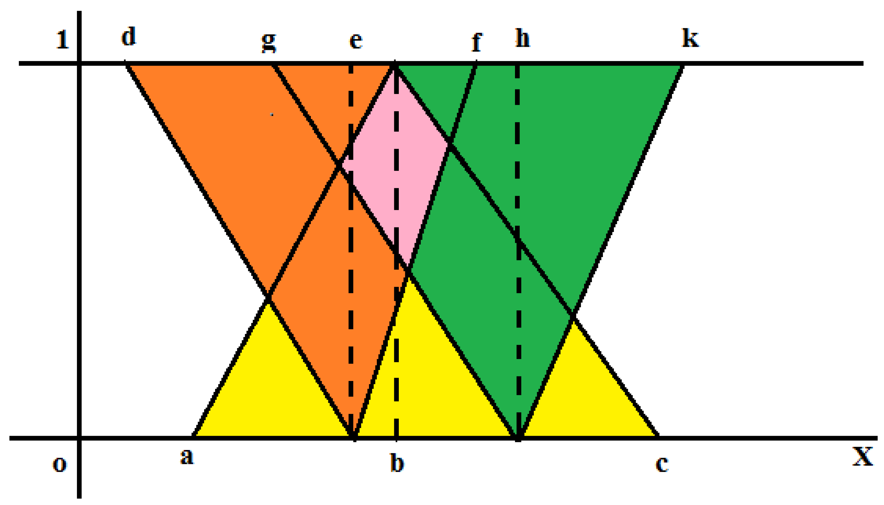
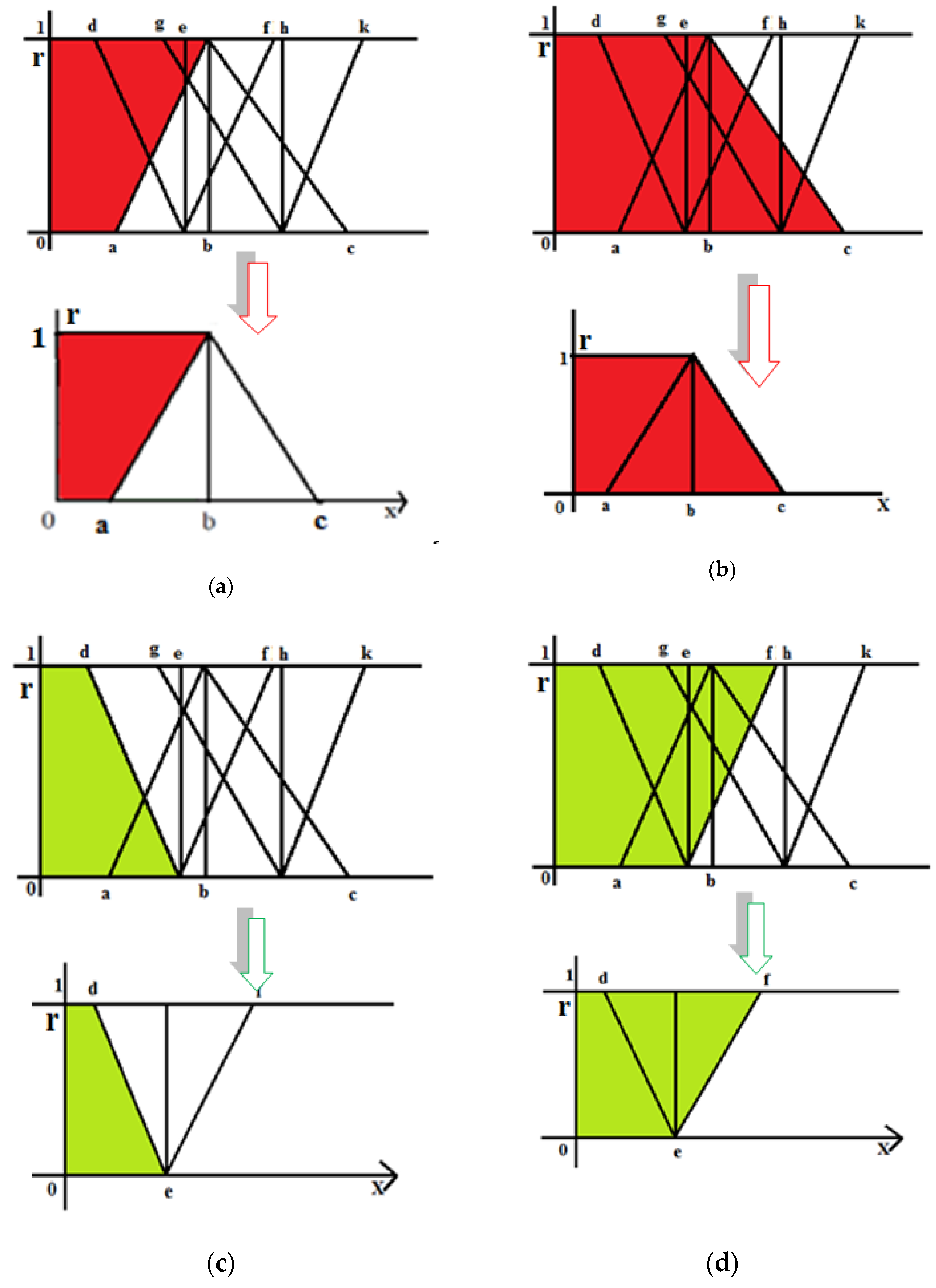
5. De-Neutrosophication of Linear Neutrosophic Triangular Fuzzy Number

De-Neutrosophication Using Removal Area Method

Let us consider a linear neutrosophic triangular fuzzy number as follows:

$${\tilde{A}}_{Ne}=(a,b,c;d,e,f;g,h,k)$$

whose pictorial representation is as follows.

Firstly, we consider the graphical representation of linear neutrosophic triangular fuzzy number in Figure 6.

We consider an ordinary number $k\in R$ and a fuzzy number $\check{A}$ for the lower triangle, then left side removal of $\check{A}$ with respect to k is $R_l(\check{A},k)$, defined as the area bounded by k and the left side of the fuzzy number $\check{A}.$ Similarly, the right side removal of $\check{A}$ with respect to k is $R_r(\check{A},k).$ Also consider an ordinary number $k\in R$ and a fuzzy number $\check{B}$ for the left most upper triangle($∆$def), then the left side removal of $\check{B}$ with respect to k is $R_l(\check{B},k)$, defined as the area bounded by k and the left side of the fuzzy number $\check{B}.$ Similarly, the right side removal of $\check{B}$ with respect to k is $R_r(\check{B},k)$. A fuzzy number $\check{C}$ for the right most upper triangle($∆$ghk), then left side removal of $\check{C}$ with respect to k is $R_l(\check{C},k)$, defined as the area bounded by k and the left side of the fuzzy number $\check{C}.$ Similarly, the right side removal of $\check{C}$ with respect to k is $R_r(\check{C},k).$

Mean is defined as $(\check{A},k)=\frac{R_l(\check{A},k)+R_r(\check{A},k)}{2}$, $R(\check{B},k)=\frac{R_l(\check{B},k)+R_r(\check{B},k)}{2}$, $R(\check{C},k)=\frac{R_l(\check{C},k)+R_r(\check{C},k)}{2}$.

Then, we defined the defuzzification of a linear neutrosophic triangular fuzzy as $R(\check{D},k)=\frac{R(\check{A},k)+R(\check{B},k)+R(\check{C},k)}{3}$.

For $k=0$,

$$\begin{gathered} R(\check{A},0)=\frac{R_l(\check{A},0)+R_r(\check{A},0)}{2} \\ R(\check{B},0)=\frac{R_l(\check{B},0)+R_r(\check{B},0)}{2} \\ R(\check{C},0)=\frac{R_l(\check{C},0)+R_r(\check{C},0)}{2} \end{gathered}$$

Then,

$$R(\check{D},0)=\frac{R(\check{A},0)+R(\check{B},0)+R(\check{C},0)}{3}$$

We take $\check{A}=(a,b,c),\check{B}=(d,e,f),\check{C}=(g,h,k)$.

Figure 7 shows the pictorial representation of de-neutrosophication.

Then,

$$\begin{gathered} R_l(\check{A},0)=\mathrm{Area}\mathrm{of}\mathrm{trapezium}\mathrm{OABR}=\frac{(a+b)}{2}.1 \\ {R}_l(\check{A},0)=\mathrm{Area}\mathrm{of}\mathrm{trapezium}\mathrm{OABR}=\frac{(a+b)}{2}.1 \\ {R}_l(\check{B},0)=\mathrm{Area}\mathrm{of}\mathrm{trapezium}\mathrm{OABR}=\frac{(d+e)}{2}.1 \\ {R}_r(\check{B},0)=\mathrm{Area}\mathrm{of}\mathrm{trapezium}\mathrm{OABR}=\frac{(e+f)}{2}.1 \\ {R}_l(\check{C},0)=\mathrm{Area}\mathrm{of}\mathrm{trapezium}\mathrm{OABR}=\frac{(g+h)}{2}.1 \\ {R}_r(C,0)=\mathrm{Area}\mathrm{of}\mathrm{trapezium}\mathrm{OABR}=\frac{(k+h)}{2}.1. \end{gathered}$$

Hence, $(\check{A},0)=\frac{(a+2b+c)}{4},R(\check{B},0)=\frac{(d+2e+f)}{4}$, $R(\check{C},0)=\frac{(g+2h+k)}{4}$.

So, $R(\check{D},0)=\frac{(a+2b+c+d+2e+f+g+2h+k)}{12}$.

Example 5.

Finding De-neutrosophication value of Neutrosophic number.

Table 4. De-neutrosophication value of Neutrosophic number.

Experiment No.	Neutrosophic Number	De-Neutrosophication Value
Set 1	$\check{\mathit{A}}=(\mathbf{1},\mathbf{2},\mathbf{3};\mathbf{0.5},\mathbf{1.5},\mathbf{2.5};\mathbf{1.2},\mathbf{2.7},\mathbf{3.5})$	2.0083
Set 2	$\check{\mathit{B}}=(\mathbf{0.5},\mathbf{1.5},\mathbf{2.5};\mathbf{0.3},\mathbf{1.3},\mathbf{2.2};\mathbf{0.7},\mathbf{1.7},\mathbf{2.2})$	1.45
Set 3	$\check{\mathit{C}}=(\mathbf{0.3},\mathbf{1.2},\mathbf{2.8};\mathbf{0.5},\mathbf{1.5},\mathbf{2.5};\mathbf{0.8},\mathbf{1.7},\mathbf{2.7})$	1.533
Set 4	$\check{\mathit{D}}=(\mathbf{1},\mathbf{3},\mathbf{5};\mathbf{0.5},\mathbf{1.5},\mathbf{2.5};\mathbf{1.2},\mathbf{2.7},\mathbf{4.5})$	2.425

shows the de-neutrosophication value of Neutrosophic number.

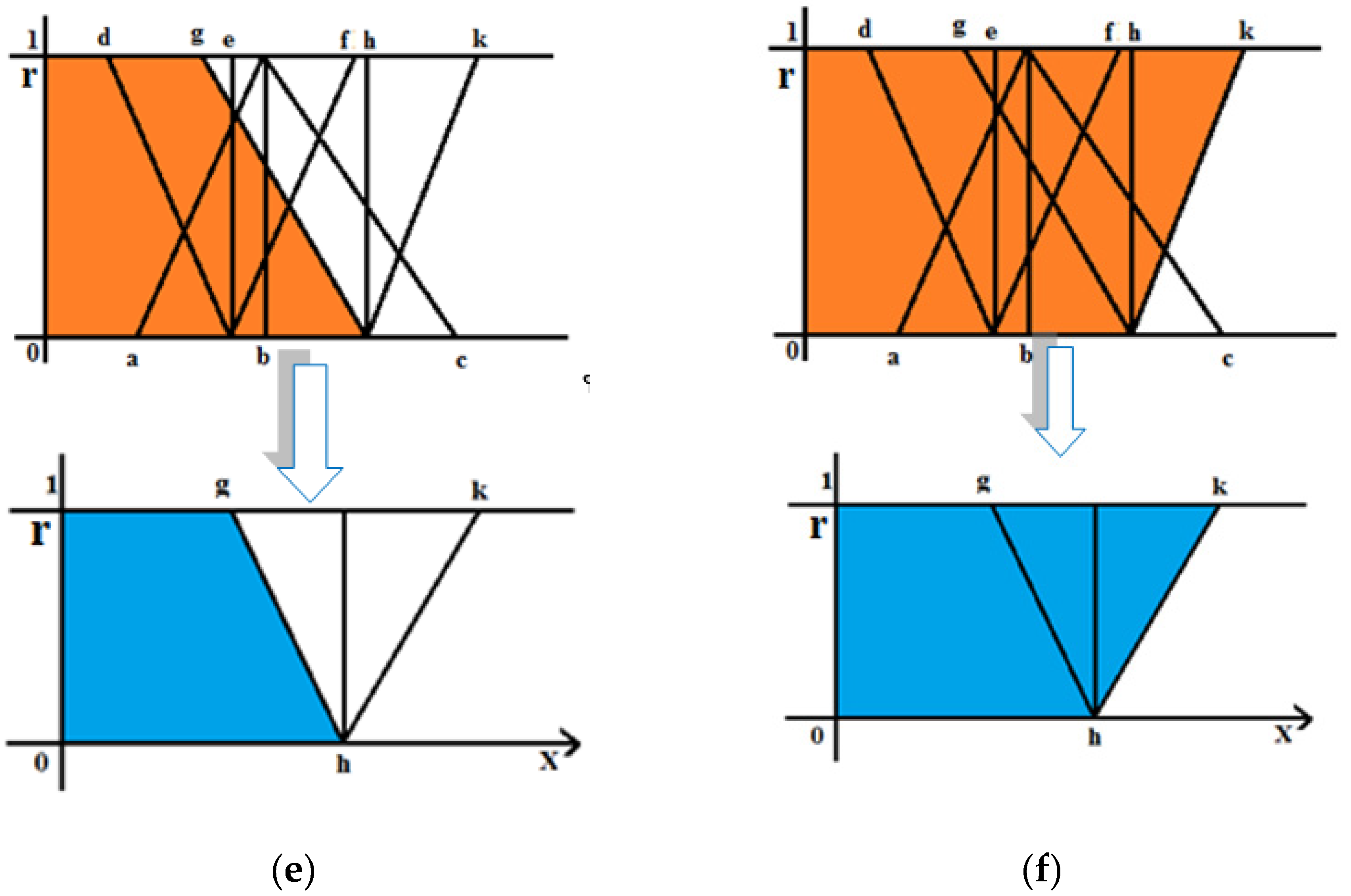
6. PERT in Triangular Neutrosophic Environment and the Proposed Model

The full form of PERT method is project evaluation and review technique, which is a project management tool used to schedule, organize, and coordinate tasks within a project. It is basically a method to analyze the tasks involved in completing a given project, especially the time needed to complete each task, and to identify the minimum time needed to complete the total project.

PERT planning involves the following steps:

• Identify the specific activities and milestones.
• Determine the proper sequence of the activities.
• Construct a network diagram.
• Estimate the time required for each activity.
• Determine the critical path.
• Update the PERT chart as the project progresses.

The main objective of PERT is to facilitate decision making and to reduce both the time and cost required to complete a project. PERT is intended for very large-scale, one-time, non-routine, complex projects with a high degree of dependency, projects which require a series of activities, some of which must be performed sequentially, and others that can be performed in parallel with other activities. PERT has been mainly used in new projects which have large uncertainty with respect to design of a structure, technology, and networking system. To take care of associated uncertainties, we introduced triangular neutrosophic environment for PERT activity duration.

The three time estimates for activity duration are as follows:

Optimistic time $(\check{o})$: Generally, the shortest time in which the activity can be completed. It is common practice to specify optimistic time to be three standards deviations from the mean so that there is approximately a 1% chance that the activity will be completed within the optimistic time.

Pessimistic time $(\check{p})$: Generally, the longest time that an activity might require. Three standard deviations from the mean are commonly used for the pessimistic time.

Most likely time $(\check{m})$: Generally, it is the completion time, in normal circumstances, having the highest probability. Note that this time is different from the expected time.

Note 2. In Ref. [22], the authors introduced the concept of score and accuracy function to compute the crisp value of a trapezoidal neutrosophic number. In our proposed model, we choose all the three different times (optimistic, pessimistic, most likely) as triangular neutrosophic number.

To obtain the crisp value, we introduced the de-neutrosophication value $R(\check{D},0)=\frac{(a+2b+c+d+2e+f+g+2h+k)}{12}$ of triangular neutrosophic number $(a,b,c;d,e,f;g,h,k)$.

Now, the expected time and standard deviation can be calculated by the formula $E_{jk}=\frac{o+4m+p}{6}$ and ${\sigma }_{jk}=\frac{p-o}{6}$, where o, p, and m are all crisp value of optimistic, pessimistic, and most likely time estimations, respectively.

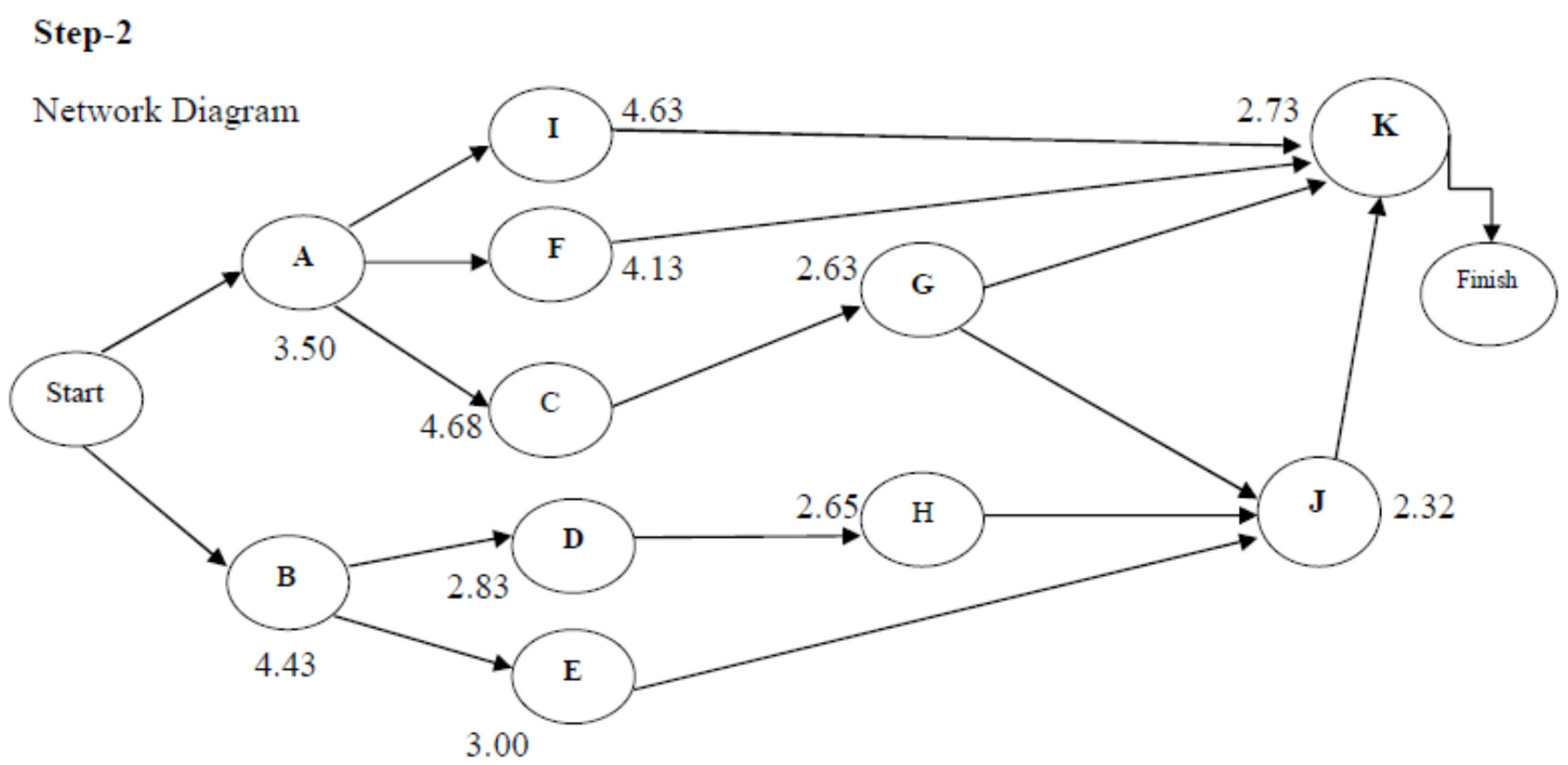
Now, we use CPM method for further calculation of earliest/latest time, critical path, and float.

In forward pass, starting with a time of zero for the first event, the computation proceeds from left to right, up to the final event. For any activity $(i,j)$, let $E{S}_i$ denote the earliest time of event $i$, then $E{S}_j=E{S}_i+t_{ij}$. If more than one activity enters an event, the earliest start time for that event is computed as $E{S}_j=\max \left\{E{S}_i+t_{ij}\right\}$ for all activities emanating from node i entering into j.

In case of backward pass, starting with the final node, the computation proceeds from right to left, up to the initial event. For any activity $(i,j)$, let $L{F}_i$ denote the latest finished time of event i, then $L{F}_i=L{F}_j-t_{ij}$. If more than one activity enters an event, the latest finish time for that event is computed as $L{F}_i=\min \left\{L{F}_j-t_{ij}\right\}$ for all activities emanating from node j entering into i.

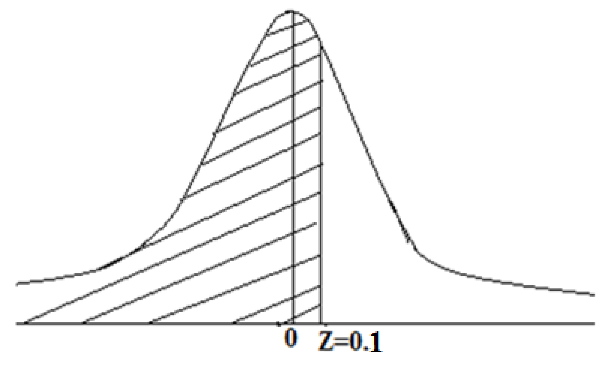
After calculating the critical path, compute project length variance, which is the sum of the variances of all the critical activities. Next, calculate the standard normal variable $Z=\frac{T_s-T_e}{\sigma }$, where $T_s$ is the scheduled time to complete the project, and $T_e$ is the normal expected project length duration. Using a normal curve, we can estimate the probability of completing the project within a specified time. The steps of the said method are shown in Figure 8. We also set the numerical value for the said problem to show the importance of our method in

Table 5. Set of Neutrosophic value of the above problem.

	Description	Predecessors	Optimistic Time	Pessimistic Time	Most Likely Time
A	Selection of Officer and Force Member	–	(1,2,3;0.5,1.5,2.5;1.2,2.7,3.5)	(1,5,9;1.5,4.5,6.5;4,7,10)	(1.5,3.5,5.5;1,2,3;3,4.5,6)
B	Selection of Site and do Site Survey	–	$(\mathbf{1},\mathbf{5},\mathbf{8};\mathbf{1},\mathbf{3},\mathbf{6};\mathbf{4},\mathbf{7},\mathbf{9})$	(1,2,3;0.5,1.5,2.5;1.5,2.5,3.5)	(1,5,8;1.5,3,6.5;4,7,9)
C	Selection of Arms	A	(1,4,7;1,3,5;3.5,6,7.5)	(1,1.5,4;0.5,1,2.5;1.25,3,4.25)	(1,5,9;1.5,4.5,6.5;4,7,10)
D	Final Plan and Blueprint	B	(1,3,5;0.5,2.5,3.5;2.5,4,6)	(1.5,3.5,5.5;1,2,3;3,4.5,6)	(0.5,2.5,4.5;1,2,3;1.5,3.5,5.5)
E	Bring Utilities to the Site	B	(0.5,2.5,4.5;0.5,1.5,3.5;2,4,6)	(1,5,9;1.5,4.5,6.5;4,7.5,10.5)	(1.5,2.5,3.5;1,1.5,3;2,3,4)
F	Interview	A	(2,4,6;1.5,2.5,3.5;3,5,7)	(1,2,3;0.5,1.5,2.5;1.2,2.7,3.5)	(1,4,7;1,3,5;3.5,6,7.5)
G	Acquisition and take delivery of arms	C	(0.5,2.5,4.5;1,2,3;2,4,6)	(1,5,8;1.5,3,6.5;4,7,9)	(1,5,9;1.5,4.5,6.5;4,7,10)
H	Construct the battlefield	D	(1.5,3.5,5.5;1,2,3;3,4.5,6)	(0.5,3.5,6.5;0.5,2.5,4.5;3,5,7)	(1,2,3;0.5,1.5,2.5;1.5,2.5,3.5)
I	Developed networking system	A	(1,5,9;1.5,4.5,6.5;4,7,10)	(0.5,2.5,4.5;1,2,3;1.5,3.5,5.5)	$(\mathbf{1},\mathbf{5},\mathbf{8};\mathbf{1},\mathbf{3},\mathbf{6};\mathbf{4},\mathbf{7},\mathbf{9})$
J	Run the system	E,G,H	(0.5,3.5,6.5;0.5,2.5,4.5;3,5,7)	(1.5,2.5,3.5;1,1.5,3;2,3,4)	(1,2,3;0.5,1.5,2.5;1.2,2.7,3.5)
K	Training for all	F,I,J	(1,5,8;1.5,3.5,6.5;4,6,8.5)	(1,4,7;1,3,5;3.5,6,7.5)	(1,1.5,4;0.5,1,2.5;1.25,3,4.25)

.

Draw the project network and find the probability that the project is completed in 16 days.

Solution. Now, we solve the problem by the following steps, as shown in

Table 6. The value of $E_{jk}$ and ${\sigma }_{jk}{}^2$ for the above problem.

Optimistic Time (o)	Pessimistic Time (p)	Most Likely Time (m)	${\mathit{E}}_{\mathit{j}\mathit{k}}\mathbf{=}\frac{\mathit{o}\mathbf{+}\mathbf{4}\mathit{m}\mathbf{+}\mathit{p}}{\mathbf{6}}$	${\mathit{\sigma }}_{\mathit{j}\mathit{k}}{}^{\mathbf{2}}\mathbf{=}{\mathbf{(}\frac{\mathit{p}\mathbf{-}\mathit{o}}{\mathbf{6}}\mathbf{)}}^{\mathbf{2}}$
2.26	5.42	3.33	3.50	0.277
4.92	2.00	4.92	4.43	0.244
4.67	1.71	5.42	4.68	0.243
2.96	3.33	2.67	2.83	0.004
2.75	5.54	2.42	3.00	0.216
3.83	2.26	4.67	4.13	0.068
2.83	4.92	2.00	2.63	0.121
3.33	3.50	2.26	2.65	0.001
5.42	2.67	4.92	4.63	0.210
3.50	2.42	2.00	2.32	0.032
4.88	4.67	1.71	2.73	0.001

, Figure 9 and Figure 10.

Step-1.

Therefore, the expected project duration is 15.9 days.

Critical path A$\to$C$\to$G$\to$J$\to$K.

Project length variance ${\sigma }^2=0.962$, standard deviation0.98.

Probability that the project will be finished within 16 days is $P(z\le \frac{16-15.9}{0.98})=P(z\le 0.1)$

Area under the normal curve $P(z\le 0.1)=0.5+\varnothing (0.1)$ = 0.5398

The related normal curve is drawn in Figure 11.

7. Application of Triangular Neutrosophic Fuzzy Number in Assignment Problem Using De-Neutrosophic Value

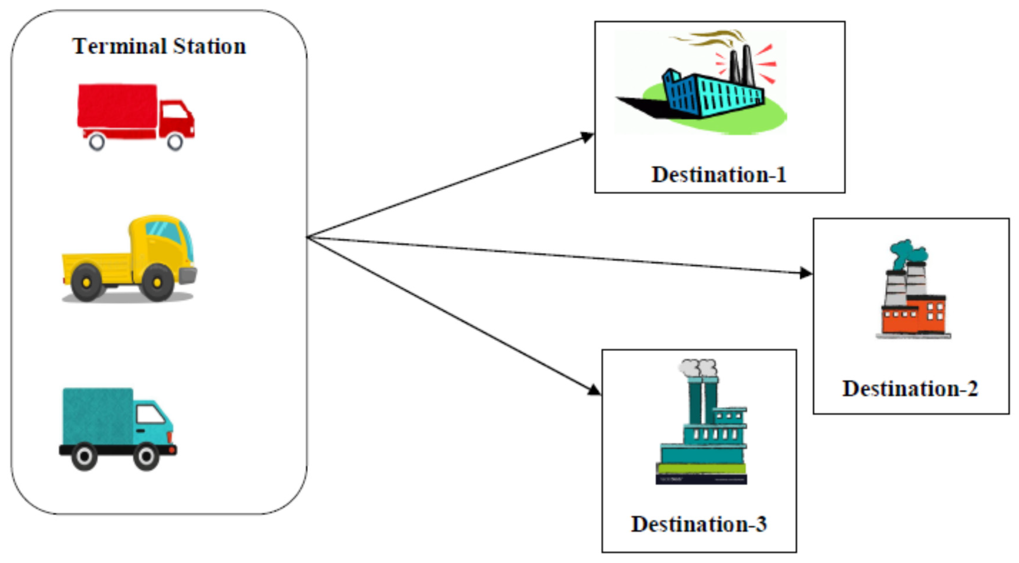
The assignment problem is very important for transferring goods from one place to another place. In the assignment problem, if uncertainty occurs, then it is more complicated to solve. By the concept of impreciseness and its corresponding crispified value, we can easily handle the assignment problem. In this section, we take a route selection problem with neutrosophic cost data and solve the problem.

We consider a problem of assigning three different trucks to three different destinations. The assigning costs that are the travelling costs in rupees are given here. How should the trucks be dispatched so as to minimize the total travelling cost? Note, that all the costs are triangular neutrosophic numbers.

Let us consider that the transportation cost for the three trucks are neutrosophic in nature. For that viewpoint, we take that the cost of the three trucks are as follows in Table 1, in units of dollar. Each component represents the moneys in units of dollars.

Here, red car denotes Truck 1, yellow car denotes Truck 2, and green car denotes Truck 3 as shown in the Figure 12.

We apply the defuzzification result of triangular neutrosophic number from

Table 7. Neutrosophic value for the transportation costs.

	Destination-1	Destination-2	Destination-3
Truck 1	(1,4,7;1,3,5;3.5,6,7.5)	(0.5,2.5,4.5;1,2,3;1.5,3.5,5.5)	(1,3,5;0.5,1.5,3.5;2,4,6)
Truck 2	(1,2,3;0.5,1.5,2.5;1.5,2.5,3.5)	(1,1.5,4;0.5,1,2.5;1.25,3,4.25)	(1.5,2.5,3.5;1,1.5,3;2,3,4)
Truck 3	(2,4,6;1.5,2.5,4.5;3,5,7)	(1,5,8;1.5,4.5,7.5;4,6.5,9)	(1,5,8;1.5,3,6.5;4,7,9)

.

$R(\check{D},0)=\frac{(a+2b+c+d+2e+f+g+2h+k)}{12}$ to convert the numbers into a crisp number.

Then, we have the following

Table 8. De-neutrosophication value for the transportation costs.

	Destination-1	Destination-2	Destination-3
Truck 1	4.25	2.67	2.92
Truck 2	2.00	1.71	2.75
Truck 3	3.92	5.25	5.08

.

Now, we consider row minimum from each row, and subtract it from the other element (row-wise). Thus, we get

Table 9. Row minimum from each row, and subtract it from the other element (row-wise).

	Destination-1	Destination-2	Destination-3
Truck 1	1.58	0	0.25
Truck 2	0.29	0	1.04
Truck 3	0	1.33	1.16

.

Now, we consider column minimum from each column and subtract it from the other element (column-wise). Thus, we get

Table 10. Column minimum from each column and subtract it from the other element (column-wise).

	Destination-1	Destination-2	Destination-3
Truck 1	1.58	0	0
Truck 2	0.29	0	0.79
Truck 3	0	1.33	0.91

.

Here, the minimum number of straight lines to cover all the zeros is 3 (which is also equal to the order of the matrix), as shown in

Table 11. Minimum number of straight lines to cover all the zeros.

	Destination-1	Destination-2	Destination-3
Truck 1	1.58	0	0
Truck 2	0.29	0	0.79
Truck 3	0	1.33	0.91

.

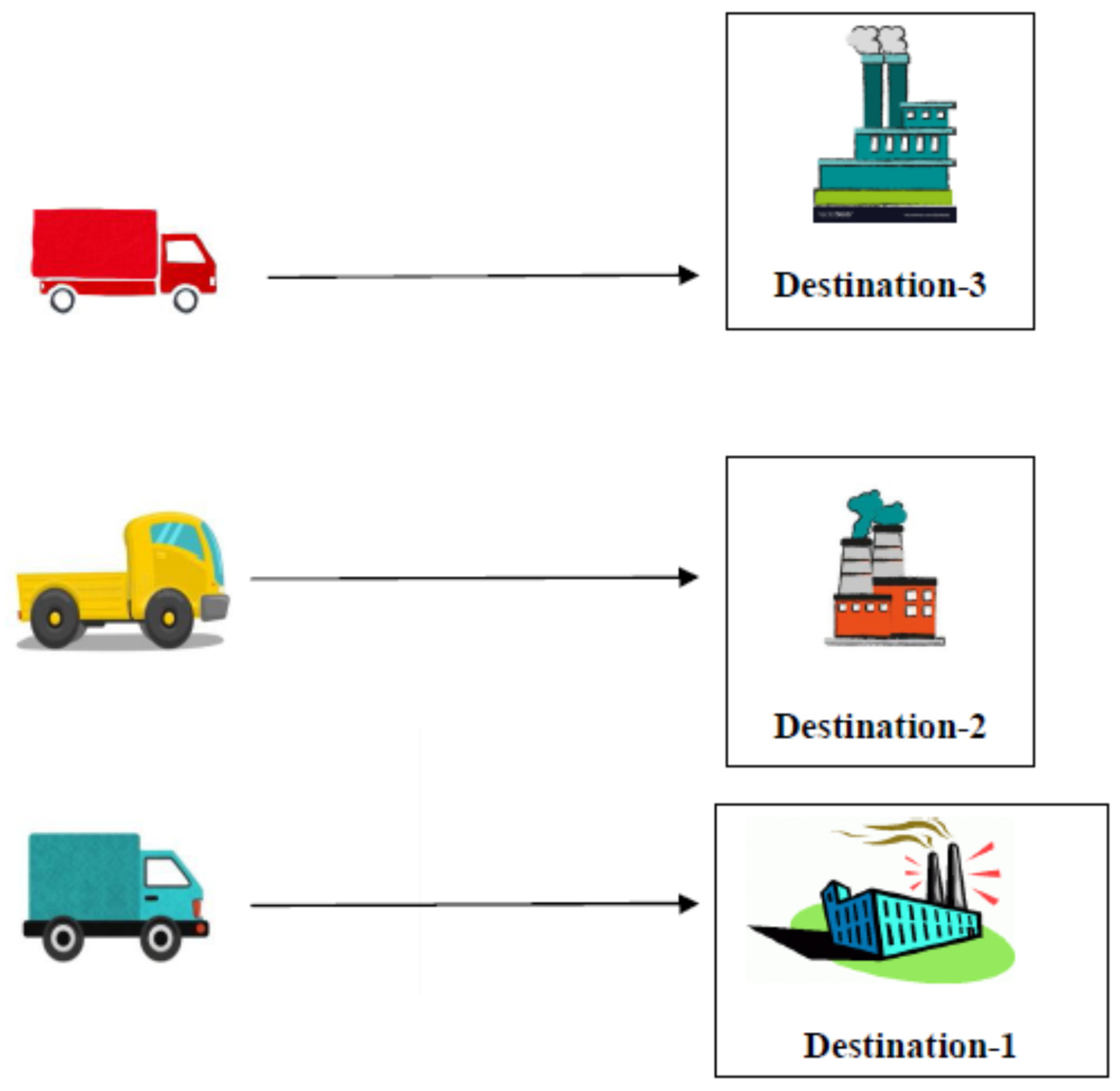
From the

Table 12. Transformed table.

	Destination-1	Destination-2	Destination-3
Truck 1	1.58	0	$\left[\mathbf{0}\right]$
Truck 2	0.29	$\left[\mathbf{0}\right]$	0.79
Truck 3	$\left[\mathbf{0}\right]$	1.33	0.91

, we see that if the Truck1 goes to Destination-3, Truck2 goes to Destination-2, and Truck3 goes to Destination-1, then the carrying is minimum.

That means from the Figure 13 Truck-1$\to$Destination-3, Truck-2$\to$Destination-2, Truck-3$\to$Destination-1.

The corresponding Min cost = (3.92 + 1.71 + 2.92) = 8.55 units of dollar.

Then, we get

Table 13. Neutrosophic value of destinations.

	Destination-1	Destination-2	Destination-3
Truck 1	(1,4,7;1,3,5;3.5,6,7.5)	(0.5,2.5,4.5;1,2,3;1.5,3.5,5.5)	(1,3,5;0.5,1.5,3.5;2,4,6)
Truck 2	(1,2,3;0.5,1.5,2.5;1.5,2.5,3.5)	(1,1.5,4;0.5,1,2.5;1.25,3,4.25)	(1.5,2.5,3.5;1,1.5,3;2,3,4)
Truck 3	(2,4,6;1.5,2.5,4.5;3,5,7)	(1,5,8;1.5,4.5,7.5;4,6.5,9)	(1,5,8;1.5,3,6.5;4,7,9)

.

Ye [21] built up the concept of score function and accuracy function. The score function S and the accuracy function H are applied to compare the grades of triangular fuzzy numbers (TFNS). These functions show that greater is the value, the greater is the TFNS, and by using these, concept paths can be ranked.

We apply the result of triangular neutrosophic number.

Let, $\check{A}=(a,b,c;d,e,f;g,h,k)$ be a triangular neutrosophic fuzzy number, then the score function is defined as $S(\check{A})=\frac{\left\{8+(a+2b+c)-(d+2e+f)-(g+2h+k)\right\}}{12}$, and accuracy function is defined as $H(\check{A})=\frac{\left\{(a+2b+c)-(g+2h+k)\right\}}{4}$.

In order to make comparisons between two triangular neutrosophic values, Ye [21] presented the order relations between two triangular neutrosophic values.

Let $\check{A_1}=(a_1,b_1,c_1;d_1,e_1,f_1;g_1,h_1,k_1)$ and $\check{A_2}=(a_2,b_2,c_2;d_2,e_2,f_2;g_2,h_2,k_2)$ be two triangular neutrosophic values, then the ranking method is defined as follows.

(i)

if $S(\check{A_1})>S(\check{A_2})$, then $\check{A_1}>\check{A_2}$

(ii)

if $S(\check{A_1})=S(\check{A_2})$ and $H(\check{A_1})>H(\check{A_2})$, then $\check{A_1}>\check{A_2}$

We apply the score function result of triangular neutrosophic number $S(\check{A})=\frac{\left\{8+(a+2b+c)-(d+2e+f)-(g+2h+k)\right\}}{12}$ to convert the numbers into a crisp number.

Then we have the following table, as shown in

Table 14. Converted the numbers into a crisp number.

	Destination-1	Destination-2	Destination-3
Truck 1	−0.92	−0.33	−0.25
Truck 2	0.00	−0.04	−0.08
Truck 3	−0.58	−1.42	−1.17

.

Take the most negative cost (−1.42), add it with all the elements of the matrix we get

Table 15. Corrosponing positive value table.

	Destination-1	Destination-2	Destination-3
Truck 1	0.50	1.09	1.17
Truck 2	1.42	1.38	1.34
Truck 3	0.84	0.00	0.25

.

Now, we consider row minimum from each row and subtract it from the other elements (row-wise). Thus, we get

Table 16. Row minimum from each row and subtract it from the other elements (row-wise).

	Destination-1	Destination-2	Destination-3
Truck 1	0	0.59	0.67
Truck 2	0.08	0.04	0
Truck 3	0.84	0	0.25

.

Now, we consider column minimum from each column, and subtract it from the other elements (column-wise). Thus, we get

Table 17. Column minimum from each column, and subtract it from the other elements (column-wise).

	Destination-1	Destination-2	Destination-3
Truck 1	0	0.59	0.67
Truck 2	0.08	0.04	0
Truck 3	0.84	0	0.25

.

Here, the minimum number of straight lines to cover all the zeros is 3(which is also equal to the order of the matrix), as shown in

Table 18. Minimum number of straight lines to cover all the zeros is 3.

	Destination-1	Destination-2	Destination-3
Truck 1	0	0.59	0.67
Truck 2	0.08	0.04	0
Truck 3	0.84	0	0.25

.

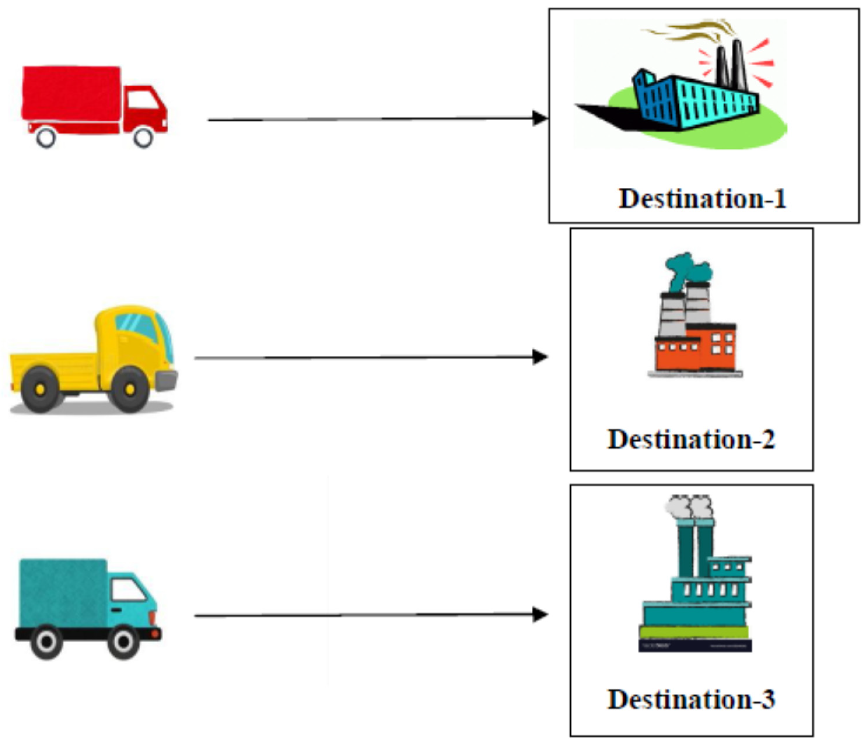
From the

Table 19. Decision table.

	Destination-1	Destination-2	Destination-3
Truck 1	[0]	0.59	0.67
Truck 2	0.08	0.04	[0]
Truck 3	0.84	[0]	0.25

, we see that if the Truck1 goes to Destination-1, Truck2 goes to Destination-3, and Truck3 goes to Destination-2, then the carrying is minimum.

That means from the Figure 14 the destination is as follows Truck1$\to$Destination-1, Truck2$\to$Destination-3, Truck3$\to$Destination-2.

The corresponding Min cost = (−0.92 − 1.42 − 0.08) = −2.42 units of dollar.

Note: Since, using de-neutrosophic value, we observe that min cost is 8.55 units of dollar, whereas using score function, we get min cost in negative quantity that is loss, hence de-neutrosophication gives us a better result than the score function.

8. Conclusions

The theory of uncertainty plays a key role in applied mathematical modeling. The concept of neutrosophic number is very popular nowadays. The formation and de-neutrosophication of the corresponding number can be very important for the researcher who deals with uncertainty and decision-making problems. In this paper, we construct the concept triangular neutrosophic number from different viewpoints, which is not defined earlier. We use the concept of linear and non-linear form with generalization of the pick value of truth, falsity, and indeterminacy functions by considering triangular neutrosophic numbers, which are very important for uncertainty theory. We introduced the de-neutrosophication concept for triangular neutrosophic numbers. This concept helps us to convert a neutrosophic number into a crisp number, which is surely helpful for decision-making problems. In future, we can extend the concept into different types of neutrosophic numbers, which can be more applicable in modeling with uncertainty.