A Review of Image Processing Techniques Common in Human and Plant Disease Diagnosis

Computer Science and Engineering Department, Technological Educational Institute of Thessaly, 41110 Larissa, Greece
Symmetry 2018, 10(7), 270; https://doi.org/10.3390/sym10070270
Submission received: 16 May 2018
/
Revised: 1 July 2018
/
Accepted: 6 July 2018
/
Published: 9 July 2018
(This article belongs to the Special Issue Advanced in Artificial Intelligence and Cloud Computing)
Abstract
:Image processing has been extensively used in various (human, animal, plant) disease diagnosis approaches, assisting experts to select the right treatment. It has been applied to both images captured from cameras of visible light and from equipment that captures information in invisible wavelengths (magnetic/ultrasonic sensors, microscopes, etc.). In most of the referenced diagnosis applications, the image is enhanced by various filtering methods and segmentation follows isolating the regions of interest. Classification of the input image is performed at the final stage. The disease diagnosis approaches based on these steps and the common methods are described. The features extracted from a plant/skin disease diagnosis framework developed by the author are used here to demonstrate various techniques adopted in the literature. The various metrics along with the available experimental conditions and results presented in the referenced approaches are also discussed. The accuracy achieved in the diagnosis methods that are based on image processing is often higher than 90%. The motivation for this review is to highlight the most common and efficient methods that have been employed in various disease diagnosis approaches and suggest how they can be used in similar or different applications.
1. Introduction
A number of disease diagnosis approaches based on a similar image processing and classification procedure are studied in this review. The referenced approaches have been selected from human and plant disease diagnosis, although many of the methods that will be presented have also been employed by similar applications like animal disease diagnosis. Similar procedure and methods can also be used in different application domains that require object recognition and classification (e.g., surveillance of protected regions, forest fire protection, weather forecast, etc.). This review has been motivated by the plant disease and skin disorder mobile applications developed recently by the author that are based on common image processing, segmentation and classification techniques. The reader can study methods that are employed in several application domains and may also be suitable for the case he is interested in. Their efficiency can be evaluated by the accuracy achieved in the experiments conducted in the referenced approaches under certain conditions. In this context, the most popular methods used for image enhancement/filtering, segmentation, and classification will be studied and directions will be given about their applicability in different cases. The application domains of the referenced approaches are introduced in the following paragraphs emphasizing on the type of the input images (visible objects, visualization of hyperspectral information, color space), their sources (cameras of visible or infrared light, MRI, ultrasound, microscope images, etc.), as well as their origin (open image databases).
The diagnosis of various human diseases can be performed though medical tests. The clinical condition of a patient is assessed by an expert that observes various types of lesions, analyzes information given by the patient, detects unusual masses through his hands, etc. Plenty of indications are given by ordinary blood, urinary tests as well as molecular analysis that can be based on biosensors [1]. Several types of sensors can also be used to monitor the condition of a person like his temperature, respiratory, blood pressure, glucose, and skin perspiration, while more advanced tests like electrocardiogram, electromyogram, etc., can also be performed [2,3]. A review of wearable systems used in rehabilitation can be found in [4]. Image processing techniques play a very important role in the diagnosis of human diseases. They can either be used to recognize the symptoms of a disease (on the skin for example) or even in the molecular analysis using microscope images that display the anatomy of the tissues. The most common disease diagnosis cases based on image processing are discussed in the following paragraphs.
Brain magnetic resonance imaging (MRI) [5,6,7,8,9,10,11] can be used for the diagnosis of glioma, AIDS dementia, Alzheimer’s, cancer metastasis, etc. The image processing is applied to T1-weighted (T1-w) and T2-w MRI scans. T1-w MRI images are obtained during the T1 relaxation time when the 63% of the original net magnetization is reached after the end of the MRI scanner radiofrequency pulse. T2-w images are obtained during T2 relaxation time, which is the time required for the decline of net magnetization to fall down to the 37% of the original net magnetization [12]. Fluid-attenuated inversion recovery (FLAIR) is an adaptive T2-w image produced when the signal of brain edema and other structures with high water content are removed [8]. Brain tumors appear with lower intensity than normal brain tissue on T1-w images and higher intensity on T2-w images. The images used in these studies have been retrieved by public databases like the Alzheimer’s Disease Neuroimaging Initiative (ADNI) [13] public database (http://adni.loni.usc.edu/), the Human Connectome Project, WU-Minn Consortium, the Open Access Series of Imaging Studies (OASIS), the Harvard Medical School MRI Database, and other local hospital databases like the Al-Kadhimiya Teaching Hospital in Baghdad, Iraq.
Image processing has also been employed in skin disorders for the classification of their symptoms. The most important skin disease is the melanoma [14,15,16,17,18,19,20,21,22,23,24,25,26,27] but several others including mycosis, warts, papillomas, eczema, acne, vitiligo, etc., can also be recognized by images displaying skin lesions. The sources of these images are ordinary cameras and they are processed in Red-Green-Blue (RGB) color space. The color particularity of the melanoma lesion is used by special color feature detection techniques that assess the variation of hues [24], the detection of color variegation [25], relative area of the skin lesion occupied by shades of reddish, bluish, grayish, and blackish areas and the number of those color shades [26]. Different color scales like spherical color coordinates and L*a*b have also been employed to separate the regions of interest (ROI) with higher precision [27]. Some of the melanoma diagnosis techniques have been implemented as smart phone applications [22,23]. The datasets of these approaches were retrieved from sources like: Skin and Cancer Associates (Plantation, FL, USA), the Dermatology Associates of Tallahassee, FL, EDRA Interactive Atlas of Dermoscopy [14], Sydney Melanoma Diagnostic Centre in Royal Prince Alfred Hospital [20], Cancer Incidence Dataset (http://www.cdc.gov/cancer/npcr/datarelease.htm#0), [22,28], Pedro Hispano Hospital (PH2 database) [23], http://www2.fc.up.pt/addi, http://www.dermoscopic.blogspot.com [15], Dermis, and Dermquest medical sites [16].
Other skin disorders can be detected by image processing applications that verify the existence of a single disease e.g., psoriasis in [29] and acne in [30,31]. Other applications discriminate between multiple skin diseases [32,33,34,35,36,37,38]. The image processing in most of these cases is performed in RGB although different color spaces have also been employed like hue saturation value (HSV), YCbCr [30]. Smart phone applications are also available for skin disorder diagnosis like those described in [31,39,40]. The dataset sources in these references are Atlas of Clinical Dermatology (Churchill Livingstone, 2002), eCureMe Online Medical Dictionary [33], UCI Repository of Machine learning databases [34,38], Dermnet Skin Disease Atlas [36], in the references of [37].
Mammograms are images used to detect breast cancer [41,42,43,44,45]. The ordinary color space of these image processing techniques is RGB. The datasets used in these references are publicly available image libraries like digital database for screening mammography (DDSM) and the mammographic image analysis society (mini-MIAS). Cardiovascular disease detection is also another domain where image processing techniques are applied on coaxial tomography (CT) scans [46]. Available image datasets for cardiovascular diseases can be retrieved by Osiris DICOM (http://www.osirix-viewer.com/datasets) [46]. Carotid arteries also offer significant information about cardiovascular diseases and ultrasound imaging can also be employed in this case [47]. Big data mining techniques can also assist the diagnosis of these diseases as described in [48]. The condition of blood vessels can be estimated by images of the eye retinal vessels captured by fundus cameras [49]. The images used in [49] were retrieved from the Digital Retinal Images for Vessel Extraction (DRIVE) dataset. Similarly, in [50], Shearlet transform and indeterminacy filtering is applied on fundus images of the retina retrieved from the DRIVE and the Structured Analysis of the Retina (STARE) databases. A different approach is presented in [51] where a 3D modeling of the human cornea is performed based on Scheimpflug tomography data. MRI T1-w/T2-w scans are also used for the evaluation of the prostate condition as described in [52]. The MRI images used in this approach were retrieved from Cannizzaro Hospital (Catania, Italy). Fat in the liver can be recognized as described in [53] where images are captured from a microscope during biopsy. The use of fuzzy logic in medical image processing applications is reviewed in [54].
Several referenced applications are based on the use of filters and thresholds to the image prior to the isolation of the lesion spots. Classification methods follow to confirm the existence of a disease or to classify an image in one of the supported diseases.
Similar techniques are also used in precision agriculture and especially plant disease recognition. Thus, various approaches from this domain are also examined. In [55], a review of smart detection methods of diseases, insect invasion etc., in crop fields is presented. Although there is no universal solution for all problems there are plenty of human disease diagnosis techniques that have also been employed for plant disease detection, too. The applications described in [55] include weed detection [56,57,58], disease diagnosis [59,60,61,62], and insect invasion [63,64]. The referenced approaches in [55] use as input, photographs that are analyzed either in RGB [58,61] color space or focusing on chlorophyll fluorescence ([57,62]), or properties in hyperspectral space ([56,59,60,63]). Vegetation Indices are defined in [65] that can be used as invariant features for the classification.
Several image processing solutions have been presented for the treatment of specific plant diseases. In [66], a low-cost machine vision method is described for the detection of Huanglongbing (HLB) disease in citrus. Τhe symptoms of Fusarium head blight in wheat fields can be detected and analyzed with spectro-optical reflectance measurements in the visible and near-infrared range [67]. Digital images of wheat fields at seedling stages with various cultivar densities are analyzed in RGB space in [68] for counting seedlings. Unmanned aerial vehicles (UAVs) have been recently employed as described in [69] where multispectral image and thermal view is used to detect if a plant with opium poppy is affected by downy mildew. In [70], UAVs are employed with a RGB camera and other sensors like a near-infrared camera. RGB to L*a*b color conversion is performed to the images retrieved. The author of the present review has recently presented a smartphone application that can diagnose plant (e.g., citrus and vine) diseases [71,72].
The separation of mature fruits is another application of image processing in precision agriculture. In [73], immature peach detection is performed by distinguishing the regions on a peach in RGB images. Automated citrus harvesting is studied in [74] where the RGB format is converted to the citrus color index (CCI) in order to classify how mature are the fruits. Pineapples and bitter melons were used in [75], for the evaluation of a texture analysis method that is used to detect green fruits on plants. Two new methods for counting automatically fruits in photographs of mango tree canopies are presented in [76] where YCbCr color space is used. One of these methods employ texture-based dense segmentation and the other is using shape-based fruit detection.
As already mentioned, an image processing technique followed by a low complexity classification method has been proposed recently by the author and has been employed in plant disease recognition and skin disorder classification. The features used in this method will be used to demonstrate many of the image processing techniques employed by other referenced approaches. Even if there is no universal solution appropriate for all cases, the steps followed in most of the referenced applications include an initial filtering that enhances the image (contrast, smoothness, edge detection, removal of noise, background separation) in order to isolate the ROIs and extract useful features used in the disease diagnosis. Color spaces different than RGB can also be employed for the same target. The segmentation process isolates ROIs that display the lesion and can be performed in grayscale using various types of thresholds or by accurately locating the boundaries of the lesion through e.g., geometrical properties, statistical processing of pixel properties in small windows, etc. The extracted ROI features serve as input to various classification techniques. The most popular of the image processing techniques used in each one of these stages will be examined in the following sections. The experimental results achieved in the referenced approaches will also be listed per category and the appropriateness of the various methods used in these approaches will be discussed.
This paper is structured as follows: in Section 2 the image processing technique for plant or skin disease diagnosis developed by the author will be briefly described. Several filtering and image enhancement methods will be discussed in Section 3. Popular segmentation methods often based on the use of thresholds will be presented in Section 4, while the classification techniques employed either for human or plant disease diagnosis will be discussed in Section 5. Finally, experimental results and discussion will follow in Section 6 and Section 7, respectively. In the following sections, an attempt has been made to assign to each symbol only one meaning throughout this paper. However, the parameters have to be treated locally with the definitions given in each method since similar symbols may not have the same meaning when used in different methods.
2. An Image Processing Technique Appropriate for Mobile Classification Applications
The framework described in this section was implemented for plant disease recognition as a mobile application (Plant Disease) [71,72]. The same classification method was also adapted in a similar mobile application called Skin Disease that has been developed for skin disorder diagnosis. In both applications, a number of features are extracted by a photograph that displays a part of a plant or human skin, respectively. These features concern the following regions: the normal part, the lesion consisting of a number of spots, a halo around the lesion spots, and the background. The set of the limits of each feature that are estimated by a simple statistical processing of a few training photographs displaying the same disease, forms a disease signature. The proposed classification method simply compares the features extracted from a new photograph with the appropriate limits defined in the disease signature.
In Figure 1, the user interface of the Plant Disease application is shown. The main page appears in Figure 1a where the user can select the photograph to be analyzed. Three threshold parameters may be modified under the photograph to separate the three regions mentioned earlier, by their brightness. The photograph then is analyzed and these regions are recognized and displayed in different gray levels (Figure 1b): the background in white, the lesion spots in black, the normal leaf in dark gray and the halo around the spots in brighter gray. Some features fi used in the classification are also listed at the bottom of the page (number of lesion spots, relative spot area, average gray level of the normal leaf and the spots). For each one of the leaf regions (spots, normal, halo), three histograms are constructed, for each one of the basic colors (R, G, B). These overlapping histograms are also presented in the main application page as shown in Figure 1c,d. They represent the number of pixels in each region that have the same color level. Since the lesion and the normal leaf have distinct colors, single lobes at different positions appear in the corresponding histograms as shown e.g., in Figure 1c. The halo is defined as a zone of Hp pixels around the spots. Thus, it may also include spot and normal leaf pixels and its histograms may not consist of a single lobe (Figure 1d). Leafs affected by the same disease are expected to have similar color features and histograms. Instead of trying to match the shape of the histograms during the classification phase, only the beginning, the end and the peak of each histogram are taken into consideration and these features are displayed in the next application page shown in Figure 1e. Additional information may be given by the author e.g., in Figure 1f where the part of the plant is selected. Meteorological information about the region where the plant was photographed, plays an important role in the plant disease diagnosis. The location of the plant can be retrieved through GPS (Figure 1f). Sites that provide information about the weather of this location in specific dates are accessed through the application page of Figure 1g. The average humidity, minimum and maximum daily temperatures are additional features used in the employed classification method.
In Table 1, the features used in the Plant and the Skin Disease applications are listed. The features not used in skin disease diagnosis are the ones that concern the weather data. All of the features derived by the image processing of the photograph are used in both applications. The gray level of the normal plant part is used in Plant Disease as a feature, but in Skin Disease it is used for the normalization of the lesion and halo brightness.
The environment of the Skin Disease application is similar to the one shown in Figure 1 and some illustrative pages are presented in Figure 2. The photograph selected in Figure 2a displays skin with papillomas. The color histogram triplets of each region appear in Figure 2c–e confirming that the histograms consist of a single lobe and thus, only the begin, the peak and the end of each lobe may be encountered by the classification method. The body part displayed in the photograph can be selected by the lists of Figure 2f,g or it could have been selected graphically as e.g., in the mole monitoring application Miiskin (http://miiskin.com).
From the 36 features listed in Table 1, we will focus arbitrarily on six of them: number of spots (f1), relative area of the spots (f2), spot gray level (f4), the lobe beginning (f6), the peak (f7), and the end (f8) of the histogram that corresponds to the red color of the spot (SR). In Table 2, the values estimated for these features are shown for a number of “training” photographs displaying citrus diseases (Alternaria, citrus chlorotic dwarf virus [CCDV], some kind of nutrient deficiency, melanose, anthracnose). Similarly, in Table 3, the values of these features are listed for a number of training photographs displaying skin disorders (vitiligo, acne, papillomas, mycosis). The mean value of each feature and its standard deviation (assuming Gaussian distribution and feature independence) are also listed in Table 2 and Table 3. The example feature values listed in these tables will be used in the demonstration of several image processing techniques.
3. Image Enhancement Filtering Methods
Several filtering methods have been proposed for the enhancement of the input image that displays the plant or body part in the disease diagnosis applications. The applied filtering methods reassure that a more accurate segmentation will follow. More specifically, they target at the precise definition of the ROI borders like the lesion spots, the background, etc. Edge sharpening may also be necessary for the highlight of the pixels that determine the borders of a region. These are usually characterized by the abrupt change in the color of their neighboring pixels. For example, if the spot on an orange fruit (see Figure 3) is brown then, a pixel whose adjacent ones are grouped in a set of orange pixels and a set of brown pixels, can be assumed that belongs to the edge. These pixels can be painted with different color in order to view easier the borders of a ROI. The corresponding filtering can be implemented as a moving window (of 3 × 3 pixels in the simplest case) where the pixels surrounding the central one are examined to see if they have the same color (either orange or brown). If some of these pixels have different color than the others, then the pixel at the center of the window is marked as edge, otherwise it is left intact.
Using the image of Figure 3, the orange color of the normal fruit is distinguished by assuming that both the red and the green components of an orange pixel are greater than the blue by a threshold T1. The dark spots are distinguished by assuming that all the color components of a spot pixel have a value lower than a second threshold T2. This method is implemented in Octave and the recognized edges are shown in Figure 3 with red color. This method is simple but is sensitive to the value of the thresholds T1, T2. As can be seen from Figure 3, a slight modification in T2 results in different estimation of the spot borders.
Fuzzy logic has also been used for edge sharpening as described in [54]. Fuzzy logic can also be employed in other stages like the segmentation and classification as will be described in the following sections. In [53], edge sharpening is also used after converting the original image to gray scale. A gray level threshold T3 can be used to segment different image areas and the pixels having gray level equal to T3 (or “T3 ± a small margin” for higher flexibility) can be assumed to be the border of a spot. The conversion of an image to gray scale can be performed either by simply averaging the basic color components or by a weighted averaging like [53]. Using Octave to demonstrate this simple T3 thresholding, we get the Figure 4a where the red dots show the recognized spot boundaries. It is obvious that this method is less accurate than the one used in Figure 3. In Figure 4b, the same image appears with normalized color as will be explained in the following paragraphs.
The conversion of an image to gray scale and then to black and white (binary mask) is performed for several purposes. In [53], the gray version of the image displaying liver tissue is subject to equalization and then a gray level threshold (similar to T3 in the previous paragraph) is used to convert the image to binary (black and white) representation. The white color corresponds to fat regions while the rest of the liver area is painted in black. In a second stage the recognized fat regions are validated according to their shape.
In [46], several image processing techniques are examined for cardiovascular biomedical applications. Gray level analysis is also employed taking into account anatomical peculiarities of the patient. Although these methods are efficient they are sensitive to gray levels variability between patients. A method is proposed that is robust to interpatient gray level and anatomical variability and it is based on two properties of parenchymal organs: homogeneous structure and relatively sharp boundaries on the images with contrast. If p(i, j) represented the spatial dependence of each pixel (i, j) then, the entropy is used in the segmentation process. Voxels inside of parenchymal organs have low entropy while the ones on the boundary have higher values due to higher variations in the intensities of its neighboring pixels. An entropy threshold is used to generate a binary mask. The active contours (AC) method follows for the accurate estimation of the borders of the parenchymal organs.
In the preprocessing stage presented in [8], the MRI scan is enhanced by Gaussian low pass filtering for noise removal, normalization of pixel intensity and histogram stretch/shift to cover all grayscale and increase contrast. A histogram threshold is used to isolate the background while mid-sagittal plane of brain is detected and corrected before feature extraction and classification. In the post processing stage that follows the classification, tumor location identification by 3D boxes based genetic algorithm is applied as well as tumor segmentation by 3D active contour without edge (ACWE).
Co-occurrence matrices that are used in many referenced approaches represent mathematically the texture features as gray level spatial dependence of texture in an image. The co-occurrence matrix can be constructed based on the orientation and distance between image pixels. Texture patterns are governed by periodic occurrence of certain gray levels. Consequently, the repetition of the same gray levels at predefined relative positions can indicate the presence of a specific texture. Several texture features such as entropy, energy, contrast and homogeneity, can be extracted from the co-occurrence matrix. A gray level co-occurrence matrix C(i, j) is defined based on a displacement vector dxy = (δx, δy). The pairs of pixels separated by dxy distance that have gray levels i and j are counted and the results are stored to C(i, j). Such a co-occurrence matrix is defined in [29] for psoriasis detection using skin color and texture features. In [36], the co-occurrence matrix is also used to classify images based on texture analysis into one of the following skin disorders: eczema, impetigo, psoriasis. Modified Gray Level Co-occurrence Matrix (MGLCM) is used in [8] where the authors proposed this second-order statistical method to generate textural features of MRI brain scans. These features are used to statistically measure the degree of symmetry between the two brain hemispheres. Bayesian coring of co-occurrence statistics are used for the restoration of bicontrast MRI data for intensity uniformity in [5].
In [40], thresholds in the gray level of the images are used to separate the background from the body part as well as the lesion from the normal skin. A mask with four levels of gray (an extension of the binary mask) is used to represent the distinguished regions (normal skin, lesion spots, halo, background) as shown in Figure 2b. Similarly, the same method is applied for plant disease diagnosis where the thresholds in the gray level are used to distinguish the normal plant part from the spots and the background as shown in Figure 1b ([71,72]). Binary masks are also used in other applications of precision agriculture. For example, in [73] an immature peach detection method is described where the image is converted to a binary mask and the round black regions correspond to the fruits that the algorithm concentrates on. In [75], the green pineapple and bitter melon fruits are detected on the plants using a texture analysis method. A binary image is created based on features that indicate the locations of candidate fruit and background pixels.
Image resizing is applied for different reasons in various approaches. The size of the biopsy image in [53] is magnified to zoom in the details. Bicubic interpolation and the weighted average of the pixels in the nearest 4-by-4 neighborhood is employed for the estimation of a new pixel value. In [8], the MRI size is reduced to 512 × 512 for lower complexity in the extraction of feature values. In the ‘‘mesh’’ feature approach adopted in [75] for lower computational overhead, the features are picked in a mesh of specific locations over the image, without considering any pixel properties. In a 640 × 480 pixel image, feature points are retrieved from every 11 pixels horizontally and vertically, returning a grid of 27840 feature points.
Noise appears in the input images as a random variation in the intensity of a small number of pixels. One way to remove noise from the input image is by Gaussian spatial low pass filtering [8]. Image smooth filtering is also used to reduce the intensity and the effect of noise. Image smoothing can be achieved through a median filter that is applied in a small window of pixels as shown in Figure 5. In the simplest median filter implementation, the central pixel of the window is replaced by the middle value of the sorted values of all the pixels in the window. Median filtering is employed in the detection of invertebrates on crops [64], in the recognition of skin diseases [38] and skin melanoma [15]. More custom techniques have been employed to remove specific artifacts from an image like hair in skin disorder diagnosis [16]. The drawback of a smoothing technique is that the edges may be blurred and thus, it may be difficult to accurately determine the borders e.g., of a lesion or a human organ. Edge sharpening techniques can be employed for reassuring that the edges will remain distinct [54].
The contrast may also be increased for more precise mapping of the ROIs. For example, linear contrast adjustment is employed in [38]. The contrast is also increased by the normalization of the intensity of the gray version of an image. For example, in Figure 6a a photograph with 2 moles is shown. The gray level of the pixels within this image is between mn = 80 and mx = 182 and is stretched in the whole gray level range (0, 255) using the following pixel gray level adaptation where gi,j is the old gray value of the pixel (i, j) and is its new value. The resulting image is shown in Figure 6b.
A similar stretching is applied in the MR imaging described in [8,52]. Stick filtering is applied to effectively remove speckle noise from MRI [52] and ultrasound [77] images. A different normalization is performed in RGB color scale where the new colors R′, G′, B′ (with values between 0 and 1) of a pixel are derived by the old ones (R, G, B) using the following equations:
This kind of color normalization has been employed in [68] where seedlings are counted in a wheat field. Relative color can also be estimated in order to moderate the effect of different lighting conditions in the images. It has also been employed in [32] where an image processing system for the detection of skin disorders is described. In the melanoma diagnosis method presented in [14], the average background skin color is subtracted from each lesion pixel. The advantages of the use of relative color include reduction (a) of the differences resulting from variation in ambient light and their respected digitization errors, (b) of the errors in digitizing images from different film types or different film processing techniques, (c) of the skin color variations among persons and races. Moreover, the relative color mimics the operation of the visual system of the mammals. This specific normalization of the color has been employed in Octave to get the image of Figure 4b.
The histograms derived by an image can provide useful information. Their definition may slightly differ in each approach. The histogram of a gray image can represent the number of pixels that have the same intensity [40,71,72]. For example, if the value of the histogram at the position 50 of the horizontal axis is 520, this means that there are 520 pixels in the image that have gray level equal to 50. In RGB color space a histogram for one of the basic colors may represent the number of pixels that have the same color level. Histograms may be normalized by dividing the number of pixels with the same color level with the total number of pixels in the image. Different histograms may be defined for each one of the segmented regions of an image [40,71,72]. Histograms like these, have already been presented in Figure 1c,d and Figure 2c–e as they appear in the Plant and Skin Disease applications developed by the author.
In [53], the generated histograms are equalized to adjust brightness in images of the liver taken from biopsy. The histogram of gradients (HOG) is defined in [15] for the imitation of brain perception of the intensity gradients distribution or edge directions. HOG is a more sophisticated type of histogram. Cells of 8 × 8 pixels are grouped in overlapping blocks of 2 × 2 cells, while the magnitude ρ(x, y) and direction γ(x, y) for the coordinates (x, y) are defined as follows:
Lx(x, y) and Ly(x, y) are the first order Gaussian derivatives of the image patch luminance I in the x and y direction respectively. The operator * is the 2D discrete convolution while σ is a scale parameter. The direction γ is discretized in 9 operational bins as shown in Figure 7. A histogram is constructed for every pixel using a local spatial window where each pixel votes with its direction weighted by its magnitude ρ(x, y). HOG-based descriptors derived by images displaying melanoma are very similar leading to a successful diagnosis as described in [15].
Histogram stretching and shifting is performed in [8] to cover all the gray scale of an MRI image and increase contrast while histogram equalization is used in [38] for skin disease diagnosis. Leaf histograms are compared to reference histograms in [66] based on similarity metrics in order to diagnose citrus HLB disease.
Several types of transforms have been employed for filtering in a different domain than the spatial one. Inverse Fourier transform has been used for the reconstruction of MR images from raw data [52]. Image features are extracted by discrete wavelet transform (DWT) in [7] for the classification of brain MR images. Haar wavelet consists of a number of square-shaped functions. The mobile melanoma diagnostic tool SkinScanc [22] decomposes the lesion in the input image to square patches through three-level Haar wavelet transform to get 10 sub-band images. Texture features are extracted by statistical measures, like mean and standard deviation, on each sub-band image. Shearlets [50] are extension of wavelets that exploit the fact that multivariate functions are governed by anisotropic features such as edges in images. Wavelets are isotropic objects that cannot be efficiently used in image filtering applications. Another type of anisotropic filtering is the anisotropic diffusion filtering (ADF) employed in [42] for breast mass segmentation. ADF is an iterative filter that reduces the noise in the image while preserving the region borders. It controls the diffusion of the color in neighboring regions by selectively equalizing or amplifying the region borders.
After the description of all these image enhancement methods, the following directions can be given. Noise can be removed using simple smoothing methods like median or low pass filtering or more advanced techniques like stick filtering if artifacts of specific shape have to be removed. Sharpening may be necessary to highlight the edges blurred by the image smoothing. The pixels belonging to the edges may be recognized by examining the value of neighboring pixels, changes in the entropy, gradient vectors, etc. Anisotropic filtering may smooth an image without blurring the edges. Image contrast can be increased by stretching the color span in order to cover the whole range and thus, provide edge sharpening. Color stretching or other normalization techniques can be used to balance the variations caused by lighting conditions, disease progression, etc. Normalization methods like histogram equalization or matching are basically defined for the contrast enhancement in gray images. There are several options in adapting these methods to color images. In the simplest case, these methods can be applied independently for each color plane but this would result in significant color alteration since the proportions of the R, G, B colors would not be preserved in each pixel. The conversion of the RGB images in other spaces like L*a*b, HSL or HSV allows the normalization methods to be applied to the intensity component of each pixel without affecting the hue of the pixel. The gray version of the image can be exploited to determine the ROIs. If the ROIs can be recognized by their brightness, simple thresholds can be used. If the texture has to be taken into consideration, co-occurrence matrices can be employed and entropy thresholds can determine the ROI borders. Gradients can also be used for ROI border detection. When the ROIs are recognized, the image can be represented in binary form where e.g., white can correspond to the ROIs and black to the background.
4. Segmentation Methods
The image enhancement and filtering methods described in the previous section prepare the segmentation process that splits an image into regions of special interest. The image can consist of two types of regions in the simplest case: the ROIs that provide the useful information for the diagnosis and the rest of the image, which can be the background. More types of regions with different significance can also be discriminated. The borders of the ROIs can be determined in various ways including thresholds, gradients, etc. The image features used for the classification concern specific properties of the ROIs in most of the cases. The features used for the classification can be specific points of interest in an image like the shape of lesion. It is obvious that there may be numerous alternative shapes that also depend on the orientation of the image, making difficult the classification of the lesion. For this reason, invariant features are extracted that can be compared against a smaller number of alternative values. The classification is less complex and more accurate if it is based on invariant features.
As already mentioned in the previous section, four regions are distinguished in [40] (skin disorders), [71,72] (plant diseases), using two gray-level thresholds: the lesions, halo around the lesions, the normal skin or leaf, and the background that is ignored. These four regions are shown in Figure 1b and Figure 2b. The invariant features that are used for the classification are the number of lesion spots and their area, the gray level of the lesion, the halo and the normal skin/leaf, histogram features like the beginning, the end and the peak of the lobes, etc. The background is assumed to be much brighter than the body skin or the plant part in these applications, thus the background pixels are recognized if their brightness exceeds a predefined threshold e.g., T4 = 220. Similar single or multilevel thresholding techniques for segmentation are employed for melanoma and skin disorder diagnosis in [24,78,79].
Otsu thresholding can be used to select an optimal threshold in the gray level histogram of an image in order to separate it in two regions i.e., the ROI and the background. The selected threshold T should minimize the intra-class variance (σ2), which is defined as a weighted sum of variances of the two classes (,):
All the possible gray levels (0.255) are tested in order to select the optimal T. For each T value that is tested, the weights w0(T), w1(T) are the sum of the probabilities of the histogram bins between 0 and T, and between T and 255, respectively: , In [15], Otsu’s method has been employed for image segmentation in each color channel R, G, B. Then, binary masks are generated for each color channel and a majority logic function is applied to produce the global lesion mask. Morphological area-opening on the segmented image is used to avoid over-segmentation. Otsu’s thresholding is also employed in the pre-processing step described in [16] for the segmentation and evaluation of skin melanoma images. It is also employed in [68] for the separation of the background in images used for counting seedlings in wheat fields.
Kapur-based thresholding is described in [16] for the segmentation of the melanoma lesion. In Kapur-based segmentation the optimal gray level threshold maximizes the overall entropy. If a number of threshold alternatives Tk are considered, the entropy of each one of the thresholds for a specific color channel C (R, G, or B) is:
where is the intensity’s level probability distribution and is the occurrence probability of each threshold Tk. As already described in the previous section, an entropy-based segmentation in gray scale, for cardiovascular biomedical applications is also presented in [46]. The statistical analysis followed in [32] for skin disease diagnosis is also based on the entropy of the image.
In plant disease diagnosis and precision agriculture, application dependent color thresholds have been employed. The automated citrus harvesting described in [74] is based on computer vision that distinguishes mature citrus fruits based on a green/blue threshold. All pixels with green/blue value above a threshold are considered to belong to a fruit. In [68], the wheat seedlings are recognized by their excessive green value combined with an Otsu threshold.
In [66] the citrus fruits are isolated in the image using Gaussian mixture density (GMD). In general, the GMD decides if a pixel i with RGB color vector vi belongs to one of the K components cq. The matrix of the color vectors of all M pixels is V = [v0, v1, …, vM−1]. The probability of a vi is
where πq are the non-negative, normalized, mixing coefficients of different Gaussian components, cq is the center vector of component q and Σq is the covariance matrix. The is the multivariate normal density:
The parameters πq, vi and Σq are estimated iteratively by the expectation maximization technique that maximizes the log-likelihood:
In [66], only two (K = 2) component-regions are taken into consideration: the leaf (pixels with much higher green channel values) and the background. Prostate gland segmentation is based on fuzzy C-means (FCM) clustering algorithm in [52]. FCM divides a set of N feature vectors vi (statistical samples in Euclidean Rn space) into C clusters similarly to the K components of [66]. A feature vector vi is assigned to a fuzzy set {Y1, Y2, …, YC} defined by the FCM algorithm instead of a specific cluster as would be the case with k-means algorithm (described in detail in the next section). A different membership grade uiq indicates how close is the vector vi to the fuzzy set Yq. The relative distance diq between the vector vi and the centroid cq of the q cluster is expressed as pixel vicinity or intensity value similarity ). The clustering algorithm that performs the image segmentation in [52] attempts to minimize the double sum: . The constant m ≥ 1 controls the fuzziness of the classification process and FCM approximates the k-means hard decision algorithm when m = 1. Several other fuzzy logic methods for image segmentation are described in [54].
As already mentioned in the previous section, the entropy is used in [46] to determine the borders of parenchymal organs in cardiovascular disease diagnosis. However, active contours are used as a second stage to correct the multiple leaks in the resulting binary mask and to estimate the 3D borders of the organs. The following equation describes the velocity of every point of the contour and is used to describe the evolution of a closed surface C(u, v; t):
The α, β are constants, ag1 is the internal force (propagation) and βκ is the external force (spatial modifier), κ is the mean curvature of the contour, g1 is the speed function computed from the input image. The is the unit normal vector. An extension to this method is called active contour without edge (ACWE) and has been applied to segment the brain tumors in volumetric MRI scans in [8]. In this paper, genetic algorithms detect dissimilar regions between the left and right brain hemispheres. Both the active contour and ACWE methods have been employed in [42] for malignant and benign mass segmentation in mammograms. Active contour segmentation techniques have also been employed in [16] for skin melanoma diagnosis. The mobile phone application for skin melanoma diagnosis presented in [22] is also using active contour segmentation. In [76], several machine vision methods based on contour segmentation have been presented for counting fruits on mango tree canopies.
A semiautomatic border determination for a melanoma is described in [14]. Points of the border are selected manually and then a closed curve is formed that minimizes the spline curve’s second derivative. The boundary area is determined as a halo around the lesion with its width expressed as a percentage of the lesion area. This halo definition is similar to the one used in [40,71,72]. The images are also analyzed morphologically in [14], examining if the number of pixels lying in a radius r of the ROI (melanoma) belong to the skin lesion and if the ratio of benign to melanoma pixels exceeds a threshold, the lesion is classified as benign otherwise, as a melanoma.
Support vector machines (SVM) and random forest (RF) are two popular methods used both for image segmentation and classification. More details about these two methods will be given in the next section. These methods are compared against deep Boltzmann machine (DBM), convolutional encoder network (CEN), patch-wise convolutional neural network (CNN) in [6] for white matter hyperintensities (WMH) segmentation on brain MRI with mild or no vascular pathology. Principal component analysis (PCA) is used along with SVM to reduce the number of features. In the DBM evaluation, 3D ROIs of 5 × 5 × 5 are used to get grayscale intensity values. The CEN is trained using one MRI slice while the CNN accepts patches as input (i.e., image segments). PCA is also used in [7] to process the features extracted by DWT in brain MR images. The use of PCA is also examined in the review regarding the detection of biotic stress in precision crop protection that is presented in [55] along with several SVM, CEN, and CNN approaches. CNN and DBM are also used in [41] where mammographic masses are recognized using deep invariant features. These features assist the deep learning architecture through deep belief networks because it is difficult to train the CNN on pixels.
In disease diagnosis where the shape of the lesion is important, geometrical rules can be employed. For example, in [53] the eccentricity Ecc and roundness Rnd of the candidate liver fat regions should be verified by the following equations:
where bh and ch are the half length of the secondary and the major axis respectively, αr is the area and pr the perimeter of the region. Eccentricity values that tend to 1 are discarded because their shape is stick-like while they represent a circle if they tend to 0. Roundness equal to 1 corresponds to a circle while lower values indicate that the shape is not round enough. In the immature peach detection approach presented in [73], the roundness of the candidate fruit regions is examined by Radial Symmetry Transform (RTS). The gradient of an image is used in RTS to locate points of high radial symmetry. The contribution of each pixel is computed from its neighboring pixels along with the direction of the gradients. The mango fruit elliptical shape is also taken into consideration in [76]: segmentation of the blob contours into arcs; and then grouping of arcs into elliptical objects that are compared with reference ones. In Cubero et al. [74], the pregrading of citrus fruits requires the estimation of their size. Instead of estimating the size of the fruit from its contour, that would require the extraction of the fruit perimeter and the estimation of the center in search of the largest or average diameter, the fruit size was estimated indirectly from the area measurement. The area is calculated as the sum of all the fruit pixels. Then, the diameter diam is estimated by the area ar enclosed by a circle:
The lesion area is also estimated by the sum of spot pixels in the plant disease and skin disorder diagnosis applications presented in [40,71,72].
As a critical discussion concerning the segmentation and feature extraction methods presented in this section it can be stated that there are simple and sophisticated thresholds that can be employed to separate the pixels of an image into multiple segments-regions. The simple constant thresholds distinguish the pixels merely by their brightness. Sophisticated thresholds like Otsu are dynamically determined minimizing the intersegment variance while the Kapur threshold is related to the overall entropy. A threshold of an individual color (or color ratio) can be used to split an image into regions of different colors. The contour shape of a region can also be examined if the ROIs should have specific geometrical properties (round, elliptical, stick, etc.) and active contour is a mathematical modeling that follows the contour of a ROI. Classification or clustering algorithms (like SVM, fuzzy-clustering, k-means, neural networks, etc.) can be employed to assign pixels in specific regions. The features used in the classification stage are related to the segments of an image. These features can be pixel values from specific positions of the image. PCA or similar methods can be used in this case to reduce the feature vector size and consequently the complexity. Invariant features are more abstract properties of the segments representing metadata and their use can lead to lower complexity and faster training.
5. Classification Methods
Indicative classification methods adopted in the referenced approaches are presented in this section. It is obvious that it is not possible to cover all the classification techniques and their alternative implementations. Emphasis is given on the machine learning methods that have been used both in human and plant disease diagnosis approaches and are based on image processing techniques. Each method can belong to one of the following two main categories: supervised and unsupervised machine learning. In supervised machine learning like support vector machines (SVM), Naïve Bayes, decision trees, k-nearest neighbor, some types of artificial neural networks (multilayer perceptron [MLP]), etc., the classifier is trained by a set of representative input/output pairs. Based on its training, a transfer function is inferred that can be used for mapping new inputs to the correct output classes. In unsupervised machine learning, the classifier is trained based on statistical analysis performed in real time operation. For example, an unsupervised machine learning method can observe the behavior of the input and generate alerts either when a pattern is repeated or when a repeated pattern is interrupted. Most of the approaches described in this section are supervised learning techniques. Typical unsupervised learning includes the expectation–maximization algorithm used in [42], some special types of neural networks like deep belief nets [41], etc.
Artificial neural networks (ANN or NN) are one of the most widespread classification techniques and there are several alternative architectures for their implementation. An ANN can be described in general as a network of interconnected nodes. The input layer consists of nodes that accept as input e.g., the features extracted after the segmentation. The output of a node is a function of its inputs and the outputs of a node layer are summed with a weight (propagation function) to drive a node in the next layer of nodes. The output layer generates the classification results that are compared with the expected output during the training of the ANN. The difference between the current results and the expected output are used as a feedback to correct various parameters in the transfer and propagation functions. This parameter correction is actually the learning process of the ANN. Convolutional ANNs are employed in [49,50] for retinal vessel characterization, in [41] for detecting mammographic masses. A feed forward back propagation neural network (FFBP-NN) is used in [21,33] for dermatological disease diagnosis. ANNs have also been used in other skin disorder classification applications: [34,36,38]. MLP has been used in [47] for cardiovascular disease diagnosis. In precision agriculture applications, ANNs have been compared with several other alternative classification techniques as described in [55,64,70,73].
The classification method followed in the Plant and Skin Disease diagnosis applications presented in [40,71,72], is a hard fuzzy set of rules where the value fi of each one of the features listed in Table 1 is compared with the strict (, ) and the loose limits (, ) defined in the signature of the disease: q. A different grade () is encountered in each case with a potentially different weight () in each disease k.
The parameter N is the number of features taken into consideration in each application (e.g., N = 36 if all the features of Table 1 are used). The image is classified in the disease class q with the highest rank Rq. This feature value comparison employed in this classification method can be extended to more than two ranges (strict and loose). In a soft fuzzy-logic implementation a mean feature value fm,i, could have been estimated by the training samples. The grade Gi given for this feature could be inversely proportional to the distance of the value of this feature in a new image with fm,i. For example, if it is known that the feature values follow a Gaussian distribution with mean fm,i and variance σ2 then the disease rank Rq could have been written as:
A fuzzy logic-based color histogram analysis technique is presented by Almubarak et al. [14] for the discrimination of benign skin lesions from malignant melanomas. Initially, color histograms similar to those described in [40,71,72] are constructed where each bin has a value that represents the number of pixels that have the same color level with the bin position. This histogram is defined by the training data. A secondary histogram is constructed based on the initial one where each bin represents the number of bins in the initial histogram that have the same value xn. The benign skin lesion from the training data is used to determine the Benign fuzzy set BF. The membership values are defined based on the secondary histogram and the membership function uB(x) denoting the fuzzy set is given as:
where xn is the bin frequency in the secondary histogram and F is the bin frequency count for full membership in the fuzzy set BF. Several other image processing applications based on fuzzy logic are referenced in [54]. Two levels of fuzzy logic are described in this paper: type 1 and type 2 fuzzy sets. Type-2 fuzzy logic is used if the problem to be treated has a high or more complex degree of uncertainty. Type-1 fuzzy sets represent imprecision with numerical values in the range (0, 1).
K-nearest neighbor (k-NN) is a simple supervised classification algorithm used in many referenced approaches. The k-nearest training samples are examined around the new sample that is assigned to the class that has the majority of training samples in the examined distance (Euclidean in most of the cases). In the general case, if f = (f1, f2, …, fN) is the set of the features of the new sample and ft,j = (f1j, f2j, …, fNj) are the training samples then, the k-nearest training samples are selected by:
The new sample is assigned to the class with the majority of training samples that have been used in the optimization target of (24). The k-NN algorithm can be demonstrated using the (f2, f3) features of the plant and skin disease diagnosis listed in Table 1. The 2D map of Figure 8 can be constructed based on the sample values of Table 2 and Table 3 for citrus diseases (Figure 8a) and skin disorders (Figure 8b), respectively. In Figure 8a, the new sample is (3, 24) and k = 4. This sample is classified by the k-NN algorithm as CCDV (samples with round mark). In the same way, in Figure 8b the new sample is (13, 129) and k = 7. The new sample is assigned to the class corresponding to the diamond marks (Acne) since three of these training samples are within the k-distance. k-NN has been used in [7] for brain tumor, in [38] for skin disease diagnosis, in [73] for immature peach detection, in [76] for counting fruits on mango tree canopies, etc.
Another popular classification technique is k-means clustering [55] which is an NP-hard problem solved by heuristic algorithms. Its aim is to cluster M samples s to k clusters cq. The members of each cluster cq should have the minimum distance by their μq mean value. The clustering is achieved by:
Using the skin disorder feature values presented in Section 2 and focusing again on the features f1, f2, the k-means clustering can be demonstrated by Figure 9. In this example, k = 4 (skin disorders: acne, mycosis, papillomas, vitiligo) and each cluster consists of five members. The greedy heuristic algorithm employed in Figure 9, started by estimating all the distances between each pair of points. The smallest distance was selected and gradually all the next four smaller distances by the first point were selected to form the first cluster. Then, a point that had not been assigned to the first cluster was selected and its four closest unused neighbors were assigned to the second cluster. This was repeated until all the points were assigned to the four clusters. The most successful clustering was achieved for acne and papillomas where four of the five samples were classified correctly. Regarding mycosis, three of the five samples and only two of the five vitiligo samples were recognized correctly. Of course, this example is given for illustration purposes only. The poor classification accuracy is explained by the fact that only two features were used. The k-means clustering algorithm has been employed in [33,38] for multiple skin disease classification (e.g., psoriasis, dermatitis, lichen planus, pityriasis, etc.), in [31] for acne detection, in the review of machine learning methods for biotic stress detection in precision crop protection [55], etc.
SVM is undoubtedly one of the most popular supervised classification techniques but it is a binary classifier and can only be used in the verification of the existence of a specific disease. During the SVM training, a hyperplane is defined that separates the two classes or in other words the samples inside or outside the class of interest. For the better comprehension of the SVM, a 2D plane is used where pairs of features are considered as coordinates and displayed as points. If the points that belong to the class of interest can be fully separated by a straight line from the rest of the points then, the straight line with the highest distance (margin) from the closest points from each side is selected by SVM. If the points in the class of interest cannot be fully separated by a straight line then, some points may be falsely assumed to belong to the opposite class. For example, focusing again only on the features (f2, f3) of Section 2, the resulting points are shown in Figure 10. It is assumed that we are only interested in detecting deficiency in citrus leaves (Figure 10a) or mycosis (Figure 10b). As can be seen from Figure 10, there is no straight line to fully separate the points belonging to the classes of interest from the rest of the points in these examples.
Following the formal SVM problem definition presented in [15], the training set Tr = {(ft,i, yi)}|yi ϵ {−1, +1}} is considered. Some points defined in Tr may be allowed to violate the margins. The SVM method is the following optimization problem:
The parameter is positive and along with the cost Ct, they add a penalty for every point that violates the margins. The hyperplane , separates the two classes while the margins are defined as and . The SVM classification method is often solved by its dual formulation expressed using a Lagrangian multiplier αi. The parameter β is expressed as . The parameters xi that uniquely define the maximum margin hyperplanes are called support vectors. SVM has been used in [15,22,23] for malignant melanoma detection, in [47] for cardiovascular disease diagnosis, in brain MRI analysis [7], in skin disease verification [30], in precision agriculture application [73,75,76] and plant disease detection [55,64].
A simple to implement classification technique is a decision tree where a number of successive comparisons of the various features with appropriate thresholds are performed as we move from the root to the leaves of the tree. The samples assigned to the leaf of a decision tree comply with all the conditions examined at the intermediate nodes. Using f2, f3 feature threshold conditions for the skin disorder case study presented in Section 2 we can define the decision tree of Figure 11a. The left branch is followed if the condition examined at a specific node is false while the right one is followed if the condition is true. Four papilloma samples (pyramid mark) are isolated in region A, if f3 is lower or equal than 99. Then, region B can be isolated by checking if f2 is smaller than 22. The three of the four samples in region B correspond to vitiligo (round marks). A last comparison of f2 with 9 can isolate region C where four of the eight samples belong to mycosis (square marks) and the D region that has the rest of the samples and can be assumed to correspond to acne (pyramids). A special form (J48) of decision tree has been employed in [7] for brain MRI analysis. It is compared with k-NN classification and the use of random forest. The use of decision trees has been employed for dermatological disease classification in [38] compared with k-NN and ANN classifiers. The classification based on multiple association rules (CMAR) is another approach based on a tree structure. Its use is demonstrated in [47] for cardiovascular disease diagnosis. In [73], the use of several classification techniques including decision and regression trees are examined in a precision agriculture application (immature peach detection). Random forests can be viewed as an averaging of multiple different decision trees derived by the same training set. The goal of the random forests is to reduce the increased variance of the decision trees. The use of random forests in the detection of biotic stress in crop protection is examined among several other classification techniques in [55].
Naïve Bayes classifier is examined in [47] for cardiovascular disease diagnosis. It has also been used in precision agriculture [73]. This classification method is based on the Bayes theorem: the probability p(Cq|f) of an image belonging to a class Cq given the feature values is equal to . A Naïve Bayes classifier assumes that the features are independent variables and the p(Cq|f) is proportional to the product of p(Cq) with all the p(fi|Cq). If Cest is the estimated class where the image belongs, then:
In the citrus disease case study of Section 2, N = 6 and K = 5. If we assume for simplicity that each one of the citrus diseases has equal probability to appear then p(Cq) = 1/K = 0.2. If we also assume Gaussian distribution of the feature values then, we can estimate each p(fi|Cq) as:
where and μi are the variance and the mean value of feature i retrieved from Table 1. If the feature values f = {5, 3, 119, 128, 148, 166} are extracted from the image of a plant part, then Table 4 displays the estimated p(fi|Cq) values and the total score of each disease. As can be seen from this table the selected citrus disorder is nutrient deficiency that achieved the highest Cest value (1.1 × 10⁻⁸). Similarly, if the feature values f = {5, 3, 186, 183, 206, 225} have been extracted by an image displaying human skin, then Table 5 displays the estimated p(fi|Cq) values and the total score of each skin disorder. The diagnosed skin disorder is papillomas in this case.
Other interesting classification methods reported in the literature include the discriminant analysis that is examined among several other techniques in [73] for precision agriculture applications. Discriminant analysis is based on the Gaussian Mixture (GMD) method described in the previous section. The scaled vocabulary tree (SVT) described in [66] for citrus disease recognition is constructed by the local descriptors extracted from images with citrus leaves. A histogram is generated for each image by quantizing the local descriptors and counting the occurrences. The image category is recognized by matching its histogram against reference histograms. The matching is based on similarity metrics.
From the previous description of several classification methods, it can be stated that a disease diagnosis application can either confirm if a specific disease is present or diagnose the most likely disease. In both cases, the decision on the presence of a disease may not be adequate. Additional parameters may have to be estimated like for example the size of a prostate gland, a brain or breast tumor, the progress level of a plant disease, etc. SVM is often used to confirm if a disease is present although the clustering algorithms that have been described can also be used for this purpose with only two classes: one that corresponds to the presence of the disease and one for its absence. SVM cannot be directly employed for the selection of one disease among multiple alternatives. Supervised learning can be used if training input/output pairs are available. Unsupervised learning can be used in disease diagnosis if such a method monitors continuously the subject of interest, recognizing the ordinary feature values as normal and then generating alerts if unusual feature values appear. Although it is obvious that such a method would be appropriate to distinguish the healthy subject from a diseased one, it could also classify the inputs with unusual feature values into groups according to their similarity. Low complexity deterministic classification algorithms are the fuzzy clustering, the k-NN, the decision trees and Naïve Bayes. K-means is a more complicated method since it is an iterative NP-hard problem. Neural networks are also complicated but they can efficiently handle problems where the classification rules are difficult to determine.
Concerning the extendibility of a classification algorithm in order to support new diseases, it can be stated that in fuzzy clustering, k-NN, decision trees and Naïve Bayes, new diseases can be determined in a more clear way. In k-NN, the central sample has to be defined from the training ones that represent the new disease. In fuzzy clustering, the membership of a sample to the new disease has to be determined. New branches have to be defined in a decision tree that end to the new disease. The rules on the path from the root to the new leaf have to reassure that an image is correctly diagnosed with the new disease. The mean and the variation of the training samples of a new disease have to be estimated in Naïve Bayes. The overhead in training a NN on a new disease is higher since hundreds of photographs and multiple instances/patches of the same photograph may need to be used at its input. In k-means, the clustering algorithm should distribute the input samples in more clusters in order to cover the new diseases.
6. Experimental Results
In this section, we focus on the efficiency of the referenced approaches. First of all the most common metrics used in the literature are discussed in Section 6.1 and then the experimental results are listed per application domain in Section 6.2.
6.1. Metrics Used to Assess the Efficiency of Disease Diagnosis Methods
The most common metrics used in most of the human and plant disease diagnosis applications are the accuracy, specificity and sensitivity. These metrics are based on the number of true positive (TP), true negative (TN), false positive (FP) and false negative (FN) samples as shown in Figure 12. The reference samples (ground truth) are separated in the group of the positive ones to a disease and the ones that are negative to that disease as shown in Figure 12a. This separation can be performed manually by an expert or using other standard golden rules. A number of the negative samples are recognized by an application as true negative (TN), but some of them will be recognized as false positive (FP). On the other hand, some of the positive samples will be correctly recognized as true positive (TP) while some of them will be recognized as false negative (FN).
The sensitivity measures how many of the positive samples have been recognized as TP, while the specificity measures how many of the negative samples have been recognized as TN:
The classification accuracy is defined as the ratio of the correctly recognized (either positive or negative) to the total number of samples:
The false positive rate (FPR) and false negative rate (FNR) measure the rate of the falsely recognized samples as follows [16]:
Dice similarity coefficient (DSC) is another statistic often used for validating medical volume (3D) segmentations [6,16,52]:
In [52] spatial distance-based metrics are presented that qualify e.g., the segmentation process of disease diagnosis applications. If the boundaries of a segmentation process are defined by the vertices A = {ai: i = 1, 2, …, Ka} and the ones used as a reference (e.g., defined by an expert) are defined by vertices Tv = {tj: j = 1, 2, …, Nt}, then the following metrics can be defined: (a) the distance d(ai, Tv) between an element ai of the contour and the point set Tv, (b) the mean absolute distance (MAD) that quantifies the average error in the segmentation process, (c) the maximum distance (MaxD) that measures the maximum difference between the two ROI boundaries, etc.
In plant disease and precision agriculture applications, custom indices (vegetation index [VI], normalized difference [VI-NDVI], vegetation atmospherically resistant index [VARI]) are used to detect the severity of a disease [55,70]. In applications where the precision in the counting is important like the number of mangos on a tree [76], alternatives to mean square error (MSE) like root MSE (RMSE) and sum square error (SSE) [29] have been used. Finally, volumetric measures like volume difference ratio (VDR) are needed in some diagnosis approaches [6]. VDR is the relative volumetric difference between the automatically and manually estimated volume of an organ or a tissue.
6.2. Experimental Results Presented in the Referenced Approaches
The experimental results presented using the metrics defined in the previous section are listed here. They are grouped in 6 general human and plant disease diagnosis categories. In Table 6, the experimental results of the skin disorder diagnosis approaches are presented. As already mentioned, photographs of skin lesions that can be captured even by a smart phone [31] are analyzed. In these references, the accuracy is the most common metric used. In [36], specificity and sensitivity is also measured. The supported skin disorders are named in the second column of Table 6 while in the 3rd column the employed classification methods are listed. The simulation results presented in [32] were generated by simulations performed in MATLAB. An educational tool (Weka) for image preprocessing and the implementation of machine learning algorithms was employed in [34]. Additional information given by the user, such as the gender and the age of a patient, lesion features like dripping, inflamed, painless, sore, rash, redness are also exploited in [21,30] for higher accuracy in the diagnosis process. The difficulties in lighting and camera distance variations are discussed in [31]. In the same reference, both unsupervised and supervised clustering is tested achieving an accuracy of 86% and 92% respectively. In the approaches where neural networks are employed, the number of nodes in the input, hidden and output layers are indicatively 16-8-6 in [34], 34-16-8-1 in [38] while in [33] the number of hidden nodes tested were between 70 and 150. A large number of input samples are used in all the approaches of Table 6, for training. In [21], 75% of the input samples are used for training, 10% for validation and 15% for testing. In [29], the results were retrieved after 20497 iterations. In [33], 2055 samples were used for training (from 250 to 500 samples/disease). Finally, the dataset used in [35] consisted of 876 samples. The ratio of training:test samples in [35] is 4:1.
The most important skin disease is the melanoma and the experimental results presented in the referenced approaches that concern the diagnosis of this type of cancer are listed separately in Table 7. Since these applications provide a binary decision of whether there is melanoma or not, SVM is widely adopted. Additional metrics are used in these approaches to assess the credibility of the performed diagnosis. It is obvious that the accuracy in these applications should be close to 100% or at least higher than 90% due to the potentially critical threat of the disease. Several mobile applications [22] have been released recently that can be used for monitoring moles and warn the user that he has to visit an expert if the mole features indicate that a melanoma may be present. In [14], relative color has been employed along with fuzzy clustering while the experimental results have been generated for various different values of the fuzzy parameter a-cut. The input images in [15] are compressed in JPEG format with 24-bit RGB color depth. 224 images were used in the simulations performed in [15], while 140 images (resized to 256 × 256 pixels) with melanoma are processed by MATLAB and skinCAD tools in [16]. In [22], the image is segmented in patches and 100 experiments were carried out for the production of the experimental results. The speed of the iPhone application developed in [22] has also been measured: a large image of 1879 × 1261 pixels required 9.71 s for segmentation and 2.75 s for classification (the whole process lasted less than 15 s). The 3/4 of the images in [23] were used for training and 1/4 of them for testing (80 images with normal moles, 80 with atypical and 40 with melanoma). The system described in [23] initially decides if the input image is benign or abnormal and then, the images recognized with abnormal moles are classified as atypical or melanoma.
Image processing techniques applied to MRI scans can reveal several diseases like brain tumors, Alzheimer’s, prostate cancer, etc. with the accuracy listed in Table 8. As can be seen in this table, some additional spatial metrics like MaxD or MAD have been employed in [52] in cases where the precision in the measurement of the size of an organ like the prostate gland has to be assessed. The accuracy in the diagnosis as well as the precision of the measurements has to be high (close to 100%) due to the critical situation of diseases like prostate cancer or a brain tumor.
In [6], 60 MRI images were tested using various classification methods as listed in the first row of Table 8. SVM, RF and DBM took roughly 26, 37 and 1341 min on average, respectively, for the training process. Whereas, it took 83, 41 and 17 s on average for SVM, RF and DBM to complete one MRI data in the testing process using a Linux server with 32 Intel(R) Xeon(R) CPU E5-2665 @ 2.40GHz processors. Five different classifiers were compared in [7]: J48 decision tree, kNN, random forest (RF), and least-squares support vector machine (LS-SVM) with polynomial and radial basis kernels. Images of 256 × 256 pixels were used as input and eight principle feature vector sets were extracted. The MRI images in [8] are resized to 512 × 512 pixels and genetic algorithms are used to generate several 3D boxes with different size and location. From each MRI brain scan, 190 descriptors are attained and these features are used by the subsequent classification to differentiate between normal and abnormal brain images. In [52], both volume and spatial-based metrics are used to evaluate the size of a prostate gland. The experimental results are compared to reference results defined manually by an expert.
Other human diseases diagnosed by image processing techniques are listed in Table 9 including breast cancer, cardiovascular diseases, etc. Different image sources are used in these cases like mammograms for breast cancer, retinal images retrieved from fundus cameras, images captured by microscopes etc. The achieved accuracy in the measurement and the diagnosis performed by these techniques is higher than 80%. In [41], invariant features for breast cancer diagnosis are extracted to provide assistance to deep-learning architecture through deep belief network (DBN) and softmax linear classifier since the CNN model cannot be easily trained directly on image pixels. The speed-up robust features (SURF) and local binary pattern variance (LBPV) descriptors were initially extracted. These features have global spatial and local texture information. SURF and LBPV descriptors are transformed into invariant features by using k-means clustering and probability density function schemes. In the third phase, the deep invariant features are constructed in supervised and unsupervised fashion through a multilayer deep learning neural network. The number of ROIs that were experimentally tested was 600 (300 benign and 300 malignant) and 40% of them were used for training while 60% for testing. Active contour (AC) methods were employed in [42] to define the borders of breast masses. The parameters of the AC models were tuned using a training set of 20 ROIs (10 benign and 10 malignant masses of various shapes, sizes, margins and brightness). Then, 100 ROIs were used for testing and the results were compared with the reference values provided by an experienced radiologist. In the cardiovascular disease diagnosis presented in [47], focus is given on a ROI image of 64 × 100 pixels. In the experiments conducted in [47], coronary arteriography was performed on 214 cardiovascular patients, half of them showing more than 50% of stenosis. In the retinal vessel bifurcation detection method presented in [49], 30 images were used for training the neural networks, and 10 for testing. The initial skeletonization is performed by applying kernel functions and then, patching follows classifying the junctions as crossings or bifurcations. 100,000 patches were extracted for training and 30,000 for testing. In the liver fat detection presented in [53], 40 images from patients with hepatitis C were tested. Biopsies were digitized using a Nikon Eclipse 50i microscope with a DS-Fi2 high-definition color camera.
The experimental results achieved in the precision agriculture applications reviewed here, are listed in Table 10. In contrast with life critical disease diagnosis methods that have to be assessed by multiple metrics, a single accuracy measurement is adequate in most of these applications. This is explained by the fact that these approaches target to the measurement of the efficiency of an automation method e.g., in the harvesting process. Finally, plant disease diagnosis applications and their experimental results are listed in Table 11. Most approaches focus on the detection of a specific disease or on the diseases of a specific plant. Diagnosis rates higher than 90% have been achieved. However, lower rates may also be acceptable depending on the severity of a disease.
The experimental conditions of some of the referenced approaches listed in Table 10 and Table 11 are explained in this paragraph. In [68], 50 images representing five wheat cultivars with five seedling densities were tested. The counting accuracy was highest (97.14%) for a wheat field with 135 × 104 ha−1 seedling density. Three immature peach detection methods were tested in [73] based on a moving window scan of the image, its binary representation and the shape of the ROIs. Seven classifiers were examined for each method trained on 58 images. Then, 104 images were used for testing. The shadow and the sunny side of the fruits were tested separately with the sunny side of the fruits recognized with lower success rate. In [74], the citrus fruits were grouped in three categories based on their citrus color index (CCI). The test set consisted of 225 Navelina orange fruits. The reference fruit values were determined by a spectrophotometer (Minolta C400) at six random points. The confusion rate in each category was also measured as shown in Table 10. The data set used in [75] was based on video (640 × 480 resolution) data of 240 pineapples and 120 bitter melons at 30 and 15 frames/s, respectively, captured by the web camera of a laptop. The images used in [76] were stored in RGB color at a resolution of 4752 × 3168 pixels. Several validation sets representing different environmental conditions were tested (different nights and lighting conditions, trees in the same or different orchards). 256 images were tested in [66], resized at 1280 × 960 pixels. The image processing was performed in MATLAB.
7. Discussion
The input images in the approaches discussed in the previous sections are often ordinary photographs that can be captured by a smart phone camera (plant disease, precision agriculture, skin disorders). Such color photographs are analyzed in visible light in most of the cases. In other human disease diagnosis approaches, X-rays, ultrasounds, CT-scans or MRI are rich sources of information that are displayed as gray images. The most common color format is RGB although in precision agriculture, color spaces like YCbCr and L*a*b may be used to highlight the features that are useful for a more precise diagnosis. A color photograph may also be displayed in HSV, HSL, L*a*b format in order to apply filtering methods like histogram equalization to their color intensity component. The conversion of a color image to gray scale allows the determination of the ROI borders through the use of alternative thresholds. Multiple thresholds can be used to split the initial image to different regions according to their brightness. More sophisticated thresholds like Otsu and Kapur can be employed in both human and plant disease diagnosis applications if the segmentation has to be performed based on variation or entropy properties. In precision agriculture as well as skin disorder diagnosis applications, custom color thresholds like specific green/blue ratio values can be defined taking into account the color particularities of specific plant parts (leaves, fruits, etc.) or skin lesions.
Hyperspectral images e.g., in NIR or specific light wavelengths like 550–560 nm, 665–675 nm, 700 nm and 800 nm can reveal significant information about plant diseases. 3D information is estimated in human disease diagnosis using multiple 2D slices in MRI, CT-scan, ultrasound imaging but several techniques have also been presented that extract 3D information from an individual 2D images like texture and depth. Information about the depth can be revealed by the shades of the objects while the texture can be recognized by repeated color patterns. Co-occurrence matrices can be exploited for the recognition of the texture or for the extraction of entropy information from 2D images. It is important to stress that several disease diagnosis methods are implemented as smart phone applications allowing low cost access to healthcare and agricultural services. Such applications can assist the early diagnosis even in the case of severe diseases like melanoma.
Ordinary filtering techniques can be used to enhance the initial image in order to achieve a more precise detection of the ROI borders. Smoothing through low pass or median filtering can be employed to reduce the noise while edge sharpening and higher contrast can preserve the borders of the ROIs. The contrast can be increased by color normalization and stretching in the whole range (0.255). Several methods can be used for color normalization like histogram equalization or specification. The use of relative color or color normalization can minimize the variegation and the effect of the lighting conditions to the properties of the analyzed photograph. If pixel values are used as features in the classification process, then subsampling may be performed to reduce the complexity. Several types of transforms can be employed to extract features that are significant for a disease diagnosis application. Fourier and wavelet transforms can be used to locate special conditions in a domain other than the spatial one. For example, the power allocated to specific light wavelengths can be a significant indication about the presence of a disease symptom. Histograms can reveal the color concentration in an image and they can provide simple similarity metrics. Ιmages that are displaying the same disease are expected to show color concentration in similar histogram positions.
The image segmentation is one of the most important stages in a disease diagnosis application because the borders of the lesion or of the regions that contain the necessary information for the diagnosis have to be determined precisely. The simplest but still quite efficient technique is the segmentation in gray level using single, multiple or more sophisticated (Otsu, Kapur) thresholds as already mentioned. These techniques have been used in almost all of the application categories examined in this paper. Thresholds can be applied directly to the gray level of the image as well as to its gradients. Thresholds in the entropy are also used in cases where the entropy is different inside and outside of the region of an organ or a lesion in order to determine its borders. Geometrical rules (like roundness and eccentricity) can be employed to verify the correct segmentation if the ROIs can be also recognized by their shape rather than their color alone. Active contour detection and its variations like ACWE have also been employed in many human and plant disease diagnosis applications. Several clustering and classification techniques can also be used in the segmentation process to separate the ROIs. Neural networks (like CNN, CEN), SVM, DBM, RF, k-mean and fuzzy C-means, etc. are ordinary methods that have been employed in the segmentation stages of the reviewed approaches. The result of the segmentation (or one of its intermediate stages) can be a binary mask where the ROIs are represented e.g., in black and the background in white.
All of the aforementioned classification or clustering techniques can obviously be exploited in the last stage of a diagnosis application where the most likely disease has to be identified. The classification is based on variant (e.g., pixel values) or preferably invariant (e.g., lesion size, gray level, etc.) features that are used as input to the classifier. In the cases where the existence of a specific disease has to be verified, SVM is the method that has often been adopted although other techniques like k-means, k-NN, etc. can also be used. On the contrary, SVM cannot be easily adapted to clustering applications where an image has to be classified in one of the multiple diseases that are supported unless each one of these diseases is examined individually by a different SVM configuration. A problem arises if the system has falsely recognized multiple diseases in the same photograph. This is not an unusual scenario especially in plant disease diagnosis, but if one disease is falsely recognized as positive, the end user would not be able to realize it since the SVM does not provide a confidence indication about its decision. The rest of the classification methods examined in this review (k-means, kNN, decision trees, RF, fuzzy clustering, neural networks), can be employed with different of course efficiency when an image has to be classified as one of the supported diseases. It is obvious from Table 6, Table 7, Table 8, Table 9, Table 10 and Table 11 that the most popular classification method is the neural networks that are employed to more than 1/3 of the referenced approaches. One of the major issues in the use of the supervised classifications methods (which are more common than the unsupervised ones) is their training. Hundreds of images or image patches have to be employed for the training in order to achieve a high accuracy in the order of 80% or 90%. In many approaches, about 3/4 of the input samples are used for training and 1/4 of them for testing. The extension of these applications to support additional diseases or the customization of those already supported can only be performed by the application developer. This is an open issue for applications where the end user (that may not be skilled in computer science) needs to have the option to improve or extend the application that he has purchased without depending on the developer that created it.
Concerning the efficiency of the major classification methods discussed, we can draw the following conclusions from Table 6, Table 7, Table 8, Table 9, Table 10 and Table 11. The various types of neural networks achieve accuracy between 80% and 99%. The accuracy of SVM ranged between 68% and 99% in the various human or plant disease diagnosis applications that were examined. Fuzzy clustering achieved a success rate between 70% and 100% in most of the cases. The accuracy of k-NN was between 30% and 88% in the three referenced approaches where it was tested. Naïve Bays achieved 48% accuracy in fruit count application and 80% in cardiovascular disease diagnosis. Finally, the accuracy of the decision trees ranged between 79% and 97% in the referenced approaches.
8. Conclusions
Several human and plant disease diagnosis approaches based on image processing were examined in this review. All of these applications follow the same steps that include the initial filtering of the input image, segmentation that separates the regions of interest, feature extraction and classification based on these features. Although each case has special requirements and needs different treatment, there are several common methods that have been adopted in both the human and plant disease diagnosis domains. Smoothing in conjunction with edge sharpening (e.g., through normalization, stretching and contrast enhancement) are needed in order to remove noise and preserve the precise organ or lesion boundaries. Subsampling and conversion to gray level is performed to reduce complexity and apply thresholds for the segmentation. Two structures are often used: histograms that indicate the concentration in specific color levels and co-occurrence matrices that can reveal texture information in 2D. Concerning the classification methods, SVM is very popular in disease verification applications while various types of neural networks are used in distinguishing several diseases. Other popular classification methods include fuzzy clustering, k-NN, k-means, decision trees, random forests, etc.
The accuracy, sensitivity and specificity are the most common metrics used. In life threatening diseases, acceptable values for these metrics are higher than 90%. In these cases, additional metrics are also employed to assess a diagnosis method with higher confidence.
9. Patents
The work presented by the author in the references [40,71,72] and was reproduced in this review is covered by the provisional patents 1008484, published: 12/05/2015 (international classification: G06K 9/00) and a recent one with application number 20170100560/8-12-2017, by OBI (Greek Patent Office).
Author Contributions
N.P. is the sole author of this review.
Funding
This research received no external funding.
Conflicts of Interest
The author declares no conflicts of interest.
References
- Georgakopoulou, K.; Spathis, C.; Petrellis, N.; Birbas, A. A Capacitive to digital Converter with Automatic Range Adaptation. IEEE Trans. Instrum. Meas. 2016, 65, 336–345. [Google Scholar] [CrossRef]
- Petrellis, N.; Kosmadakis, I.; Vardakas, M.; Gioulekas, F.; Birbas, M.; Lalos, A. Compressing and Filtering Medical Data in a Low Cost Health Monitoring System. In Proceedings of the 21st PCI 2017, Larissa, Greece, 28–30 September 2017. [Google Scholar]
- Zhang, Y.; Sun, L.; Song, H.; Cao, X. Ubiquitous WSN for Healthcare: Recent Advances and Future Prospects. IEEE Internet Things J. 2014, 1, 311–318. [Google Scholar] [CrossRef]
- Patel, S.; Park, H.; Bonato, P.; Chan, L.; Rodgers, M. A review of wearable sensors and systems with application in rehabilitation. J. Neuro Eng. Rehabil. 2012, 9, 21. [Google Scholar] [CrossRef] [PubMed] [Green Version]
- Hadjidemetriou, S.; Psychogios, M.N.; Lingor, P.; Von Eckardstein, K. Restoration of Bi-Contrast MRI Data for Intensity Uniformity with Bayesian Coring of Co-Occurrence Statistics. J. Imaging 2017, 3, 67. [Google Scholar] [CrossRef]
- Rachmadi, M.F.; Valdés-Hernández, M.; Agan, M.L.F.; Komura, T. Deep Learning vs. Conventional Machine Learning: Pilot Study of WMH Segmentation in Brain MRI with Absence or Mild Vascular Pathology. J. Imaging 2017, 3, 66. [Google Scholar] [CrossRef]
- Siddiqui, M.F.; Mujtaba, G.; Reza, A.W.; Shuib, L. Multi-Class Disease Classification in Brain MRIs Using a Computer-Aided Diagnostic System. Symmetry 2017, 9, 37. [Google Scholar] [CrossRef]
- Hasan, A.; Meziane, F.; Aspin, R.; Jalab, H. Segmentation of Brain Tumors in MRI Images Using Three-Dimensional Active Contour without Edge. Symmetry 2016, 8, 132. [Google Scholar] [CrossRef]
- Das, S.; Chowdhury, M.; Kundu, M.K. Brain MR image classification using multiscale geometric analysis of Ripplet. Prog. Electromagn. Res. 2013, 137, 1–17. [Google Scholar] [CrossRef]
- Verma, R.; Zacharaki, E.I.; Ou, Y.; Cai, H.; Chawla, S.; Lee, S.-K.; Melhem, E.R.; Wolf, R.; Davatzikos, C. Multiparametric tissue characterization of brain neoplasms and their recurrence using pattern classification of mr images. Acad. Radiol. 2008, 15, 966–977. [Google Scholar] [CrossRef] [PubMed]
- Corso, J.J.; Sharon, E.; Dube, S.; El-Saden, S.; Sinha, U.; Yuille, A. Efficient multilevel brain tumor segmentation with integrated bayesianmodel classification. IEEE Trans. Med. Imaging 2008, 27, 629–640. [Google Scholar] [CrossRef] [PubMed]
- Dougherty, G. Digital Image Processing for Medical Applications; Cambridge University Press: Cambridge, UK, 2009. [Google Scholar]
- Weiner, M.W.; Veitch, D.P.; Aisen, P.S.; Beckett, L.A.; Cairns, N.J.; Green, R.C.; Harvey, D.; Jack, C.R.; Jagust, W.; Liu, E.; et al. The Alzheimer’s Disease Neuroimaging Initiative: A review of papers published since its inception. Alzheimers Dement. 2012, 8, S1–S68. [Google Scholar] [CrossRef] [PubMed] [Green Version]
- Almubarak, H.; Joe Stanley, R.; Stoecker, W.; Moss, R. Fuzzy Color Clustering for Melanoma Diagnosis in Dermoscopy Images. Information 2017, 8, 89. [Google Scholar] [CrossRef]
- Bakheet, S. An SVM Framework for Malignant Melanoma Detection Based on Optimized HOG Features. Computation 2017, 5, 4. [Google Scholar] [CrossRef]
- Dey, N.; Rajinikanth, V.; Ashour, A.; Tavares, J.M.R.M. Social Group Optimization Supported Segmentation and Evaluation of Skin Melanoma Images. Symmetry 2018, 10, 51. [Google Scholar] [CrossRef]
- Elgamal, M. Automatic Skin Cancer Images Classification. Int. J. Adv. Comput. Sci. Appl. 2013, 4, 287–294. [Google Scholar] [CrossRef]
- Sheha, M.A.; Mabrouk, M.S.; Sharawy, A. Automatic detection of melanoma skin cancer using texture analysis. Int. J. Comput. Appl. 2012, 42, 22–26. [Google Scholar] [CrossRef]
- Landau, M.; Matz, H.; Ethel, T.; Dvir, M.; Brenner, S. Computerized system to enhance the clinical diagnosis of pigmented cutaneous malignancies. Int. J. Dermatol. 1999, 38, 443–446. [Google Scholar] [CrossRef] [PubMed]
- Lau, H.T.; Al-Jumaily, A. Automatically Early Detection of Skin Cancer: Study Based on Neural Network. In Proceedings of the 2009 International Conference of Soft Computing and Pattern Recognition SOCPAR’09, Malacca, Malaysia, 4–7 December 2009. [Google Scholar]
- Bhardwaj, A.; Bhatia, J.S. An Image Segmentation Method for Early Detection and Analysis of Melanoma. IOSR J. Dent. Med. Sci. 2014, 13, 18–22. [Google Scholar] [CrossRef]
- Wadhawan, T.; Situ, N.; Lancaster, K.; Yuan, X.; Zouridakis, G. SkinScanc: A Portable Library for Melanoma Detection on Handheld Devices. In Proceedings of the IEEE International Symposium on Biomedical Imaging, Chicago, IL, USA, 20 March–2 April 2011. [Google Scholar]
- Joseph, S.; Panicker, J.R. Skin Lesion Analysis System for Melanoma Detection with an Effective Hair Segmentation Method. In Proceedings of the International Conference on Information Science (ICIS), Kochi, India, 12–13 August 2016. [Google Scholar]
- Santy, A.; Joseph, R. Segmentation Methods for Computer Aided Melanoma Detection. In Proceedings of the Global Conference on Communication Technologies (GCCT), Thuckalay, India, 23–24 April 2015. [Google Scholar]
- Umbaugh, S.E.; Moss, R.H.; Stoecker, W.V. Automatic color segmentation of images with application to detection of variegated coloring in skin tumors. IEEE Eng. Med. Biol. Mag. 1989, 8, 43–50. [Google Scholar] [CrossRef] [PubMed]
- Ganster, H.; Pinz, A.; Röhrer, R.; Wildling, E.; Binder, M.; Kittler, H. Automated melanoma recognition. IEEE Trans. Med. Imaging 2001, 20, 233–239. [Google Scholar] [CrossRef] [PubMed] [Green Version]
- Ercal, F.; Chawla, A.; Stoecker, W.V.; Lee, H.C.; Moss, R.H. Neural network diagnosis of malignant melanoma from color images. IEEE Trans. Biomed. Eng. 1994, 41, 837–845. [Google Scholar] [CrossRef] [PubMed]
- Argenziano, G.; Soyer, S.P.; Giorgi, V.D.; Piccolo, D.; Carli, P.; Delfino, M.; Ferrari, A.; Wellenhof, R.; Massi, D.; Mazzocchetti, G.; et al. Dermoscopy: A Tutorial; EDRA: St. Paul, MN, USA, 2000. [Google Scholar]
- Al Abbadi, N.K.; Dahir, N.S.; Al-Dhalimi, M.A.; Restom, H. Psoriasis Detection Using Skin Color and Texture Features. J. Comput. Sci. 2010, 6, 648–652. [Google Scholar] [CrossRef]
- Kabari, l.G.; Bakpo, F.S. Diagnosing skin diseases using an artificial neural network. In Proceedings of the IEEE International Conference of Adaptive Science & Technology, Accra, Ghana, 14–16 January 2009. [Google Scholar] [CrossRef]
- Alamdari, N.; Tavakolian, K.; Alhashim, M.; Fazel-Rezai, R. Detection and Classification of Acne Lesions in Acne Patients: A Mobile Application. In Proceedings of the 2016 IEEE International Conference on Electro Information Technology (EIT), Grand Forks, ND, USA, 19–21 May 2016. [Google Scholar]
- Ambad, P.S.; Shirsat, A.S. An Image analysis System to Detect Skin Diseases. OSR J. VLSI Signal Process. 2016, 6, 17–25. [Google Scholar] [CrossRef]
- Arifin, M.S.; Kibria, M.G.; Firoze, A.; Ashraful Amin, M.; Yan, H. Dermatological Disease Diagnosis Using Colour-skin Images. In Proceedings of the International Conference on Machine Learning and Cybernetics, Xi’an, China, 15–17 July 2012. [Google Scholar] [CrossRef]
- Abdul-Rahman, S.; Norhan, A.K.; Yusoff, M.; Mohamed, A.; Mutalib, S. Dermatology Diagnosis with Feature Selection Methods and Artificial Neural Network. In Proceedings of the IEEE EMBS International Conference on Biomedical Engineering and Sciences, Langkawi, Malaysia, 17–19 December 2012. [Google Scholar]
- Das, N.; Pal, A.; Mazumder, S.; Sarkar, S.; Gangopadhyay, D.; Nasipuri, M. An SVM based skin disease identification using Local Binary Patterns. In Proceedings of the 3rd International Conference on Advances in Computing and Communications, Cochin, India, 29–31 August 2013. [Google Scholar]
- Islam, N.; Gallardo-Alvarado, J.G.; Abu, M.; Aneem Salman, N.; Rengan, S.P.; Said, S. Skin disease recognition using texture analysis. In Proceedings of the IEEE International Conference on Control and System Graduate Research Colloquium (ICSGRC), Shah Alam, Malaysia, 4–5 August 2017. [Google Scholar]
- Kolkur, S.; Kalbande, D.R. Survey of Texture Based Feature Extraction for Skin Disease Detection. In Proceedings of the International Conference on Business Industry & Government (ICTBIG), Indore, India, 18–19 November 2016. [Google Scholar]
- Kumar, V.B.; Kumar, S.S.; Saboo, V. Dermatological Disease Detection Using Image Processing and Machine Learning. In Proceedings of the International Conference on Artificial Intelligence and Pattern Recognition (AIPR), Lodz, Poland, 19–21 September 2016. [Google Scholar]
- Adamu, A.H.; Akin-Bashiru, T.; Salleh, N. Dermedys: Android-based dermatological diagnostic and analytic expert system. In Proceedings of the Information Technology (ICIT), Amman, Jordan, 17–18 May 2017. [Google Scholar]
- Petrellis, N. Using Color Signatures for the Classification of Skin Disorders. In Proceedings of the IEEE International Conference on Modern Circuits and Systems Technology (MOCAST), Thessaloniki, Greece, 7–9 May 2018. [Google Scholar]
- Abbas, Q. DeepCAD: A Computer-Aided Diagnosis System for Mammographic Masses Using Deep Invariant Features. Computers 2016, 5, 28. [Google Scholar] [CrossRef]
- Ciecholewski, M. Malignant and Benign Mass Segmentation in Mammograms Using Active Contour Methods. Symmetry 2017, 9, 277. [Google Scholar] [CrossRef]
- Pereira, D.C.; Ramos, R.P.; Do Nascimento, M.Z. Segmentation and detection of breast cancer in mammograms combining wavelet analysis and genetic algorithm. Comput. Methods Progr. Biomed. 2014, 114, 88–101. [Google Scholar] [CrossRef] [PubMed]
- Cordeiro, F.R.; Santos, W.P.; Silva-Filho, A.G. An adaptive semi-supervised Fuzzy GrowCut algorithm to segment masses of regions of interest of mammographic images. Appl. Soft Comput. 2016, 46, 613–628. [Google Scholar] [CrossRef]
- Martins, L.D.O.; Junior, G.B.; Silva, A.C.; Paiva, A.C.D.; Gattass, M. Detection of Masses in Digital Mammograms using K-means and Support Vector Machine. Electron. Lett. Comput. Vis. Image Anal. 2009, 8, 39–50. [Google Scholar] [CrossRef]
- Danilov, A.; Pryamonosov, R.; Yurova, A. Image Segmentation for Cardiovascular Biomedical Applications at Different Scales Alexander. Computation 2016, 4, 35. [Google Scholar] [CrossRef]
- Kim, H.; Ishag, M.I.M.; Piao, M.; Kwon, T.; Ryu, K.H. A Data Mining Approach for Cardiovascular Disease Diagnosis Using Heart Rate Variability and Images of Carotid Arteries. Symmetry 2016, 8, 47. [Google Scholar] [CrossRef]
- Han, S.H.; Kim, K.O.; Cha, E.J.; Kim, K.A.; Shon, H.S. System Framework for Cardiovascular Disease Prediction Based on Big Data Technology. Symmetry 2017, 9, 293. [Google Scholar] [CrossRef]
- Pratt, H.; Williams, B.M.; Ku, J.Y.; Vas, C.; McCann, E.; Al-Bander, B.; Zhao, Y.; Coenen, F.; Zheng, Y. Automatic Detection and Distinction of Retinal Vessel Bifurcations and Crossings in Color Fundus Photography. J. Imaging 2018, 4, 4. [Google Scholar] [CrossRef]
- Guo, Y.; Budak, U.; Sengür, A.; Smarandache, F. A Retinal Vessel Detection Approach Based on Shearlet Transform and Indeterminacy Filtering on Fundus Images. Symmetry 2017, 9, 235. [Google Scholar] [CrossRef]
- Bataille, L.; Cavas-Martínez, F.; Fernández-Pacheco, D.G.; Cañavate, F.J.F.; Alio, J.L. A Study for Parametric Morphogeometric Operators to Assist the Detection of Keratoconus. Symmetry 2017, 9, 302. [Google Scholar] [CrossRef]
- Rundo, L.; Militello, C.; Russo, G.; Garufi, A.; Vitabile, S.; Gilardi, M.C.; Mauri, G. Automated Prostate Gland Segmentation Based on an Unsupervised Fuzzy C-Means Clustering Technique Using Multispectral T1w and T2w MR Imaging. Information 2017, 8, 49. [Google Scholar] [CrossRef]
- Tsiplakidou, M.; Tsipouras, M.G.; Giannakeas, N.; Tzallas, A.T.; Manousou, P. Automated Detection of Liver Histopathological Findings Based on Biopsy Image Processing. Information 2017, 8, 36. [Google Scholar] [CrossRef]
- Castillo, O.; Sanchez, M.A.; Gonzalez, C.I.; Martinez, G.E. Review of Recent Type-2 Fuzzy Image Processing Applications. Information 2017, 8, 97. [Google Scholar] [CrossRef]
- Behmann, J.; Mahlein, A.K.; Rumpf, T.; Romer, C.; Plumer, L. A review of advanced machine learning methods for the detection of biotic stress in precision crop protection. Prec. Agric. 2015, 16, 239–260. [Google Scholar] [CrossRef]
- Karimi, Y.; Prasher, O.S.; Patel, R.M.; Kim, H.S. Application of support vector machine technology for weed and nitrogen stress detection in corn. Comput. Electron. Agric. 2006, 51, 99–109. [Google Scholar] [CrossRef]
- Panneton, B.; Guillaume, S.; Roger, J.-M.; Samson, G. Improved discrimination between monocotyledonous and dicotyledonous plants for weed control based on the blue-green region of ultraviolet-induced fluorescence spectra. Appl. Spectrosc. 2012, 64, 30–36. [Google Scholar] [CrossRef] [PubMed]
- Ahmed, F.; Al-Mamun, H.A.; Bari, H.A.S.M.; Hossain, E.; Kwan, P. Classification of crops and weeds from digital images: A support vector machine approach. Crop Prot. 2012, 40, 98–104. [Google Scholar] [CrossRef]
- Moshou, D.; Bravo, C.; Oberti, R.; West, J.; Bodria, L.; McCartney, A.; Ramon, H. Plant disease detection based on data fusion of hyper-spectral and multi-spectral fluorescence imaging using kohonen maps. Real Time Imaging J. 2005, 11, 75–83. [Google Scholar] [CrossRef]
- Moshou, D.; Bravo, C.; Oberti, R.; West, J.S.; Ramon, H.; Vougioukas, S.; Bochtis, D. Intelligent multisensor system for the detection and treatment of fungal diseases in arable crops. Biosyst. Eng. 2011, 108, 311–321. [Google Scholar] [CrossRef]
- Camargo, A.; Smith, J.S. Image pattern classification for the identification of disease causing agents in plants. Comput. Electron. Agric. 2009, 66, 121–125. [Google Scholar] [CrossRef]
- Wetterich, C.B.; Kumar, R.; Sankaran, S.; Junior, J.B.; Eshani, R.; Marcassa, L.G. A comparative study on application of computer vision and fluorescence imaging spectroscopy for detection of Huanglongbing citrus disease in the USA and Brazil. J. Spectrosc. 2013, 2013, 941738. [Google Scholar] [CrossRef]
- Mirik, M.; Michels, G.J., Jr.; Kassymzhanova-Mirik, S.; Elliott, N.C. Reflectance characteristics of Russian wheat aphid (Hemiptera: Aphididae) stress and abundance in winter wheat. Comput. Electron. Agric. 2007, 57, 123–134. [Google Scholar] [CrossRef]
- Liu, H.; Lee, S.-H.; Chahl, J.S. A review of recent sensing technologies to detect invertebrates on crops. Prec. Agric. 2017, 18, 635–666. [Google Scholar] [CrossRef]
- Jensen, J.R. Remote Sensing of the Environment: An Earth Resource Perspective; Kaveney, D., Ed.; Prentice Hall: Upper Saddle River, NJ, USA, 2007. [Google Scholar]
- Deng, X.L.; Li, Z.; Deng, X.-L.; Hong, T.-S. Citrus disease recognition based on weighted scalable vocabulary tree. Prec. Agric. 2014, 15, 321–330. [Google Scholar] [CrossRef]
- Bauriegel, E.; Herppich, W.B. Hyperspectral and Chlorophyll Fluorescence Imaging for Early Detection of Plant Diseases, with Special Reference to Fusarium spec. Infections on Wheat. Agriculture 2014, 4, 32–57. [Google Scholar] [CrossRef] [Green Version]
- Liu, T.; Wu, W.; Chen, W.; Sun, C.; Zhu, X.; Guo, W. Automated image-processing for counting seedlings in a wheat field. Prec. Agric. 2016, 17, 392–406. [Google Scholar] [CrossRef]
- Calderon, R.; Montes-Borrego, M.; Landa, B.B.; Navas-Cortes, J.A.; Zarco-Tejada, P.J. Detection of downy mildew of opium poppy using high-resolution multi-spectral and thermal imagery acquired with an unmanned aerial vehicle. Prec. Agric. 2014, 15, 639–661. [Google Scholar] [CrossRef] [Green Version]
- Ballesteros, R.; Ortega, J.F.; Hernandez, D.; Moreno, M.A. Applications of georeferenced high-resolution images obtained with unmanned aerial vehicles. Part I: Description of image acquisition and processing. Prec. Agric. 2014, 15, 579–592. [Google Scholar] [CrossRef]
- Petrellis, N. Mobile Application for Plant Disease Classification Based on Symptom Signatures. In Proceedings of the 21st Panhellenic Conference on Informatics-PCI, Larissa, Greece, 28–30 September 2017. [Google Scholar]
- Petrellis, N. A Smart Phone Image Processing Application for Plant Disease Diagnosis. In Proceedings of the IEEE International Conference on Modern Circuits and Systems Technology (MOCAST), Thessaloniki, Greece, 4–6 May 2017. [Google Scholar]
- Kurtulmus, F.; Lee, W.S.; Vardar, A. Immature peach detection in colour images acquired in natural illumination conditions using statistical classifiers and neural network. Prec. Agric. 2014, 15, 57–79. [Google Scholar] [CrossRef]
- Cubero, S.; Aleixos, N.; Albert, F.; Torregrosa, A.; Ortiz, C.; Garcıa-Navarrete, O.; Blasco, J. Optimised computer vision system for automatic pre-grading of citrus fruit in the field using a mobile platform. Prec. Agric. 2014, 15, 80–94. [Google Scholar] [CrossRef]
- Chaivivatrakul, S.; Dailey, M.N. Texture-based fruit detection. Prec. Agric. 2014, 15, 662–683. [Google Scholar] [CrossRef]
- Qureshi, W.S.; Payne, A.; Walsh, K.B.; Linker, R.; Cohen, O.; Dailey, M.N. Machine vision for counting fruit on mango tree canopies. Prec. Agric. 2016, 18, 224–244. [Google Scholar] [CrossRef]
- Czerwinski, R.N.; Jones, D.L.; O’Brien, W.D. Line and boundary detection in speckle images. IEEE Trans. Image Process. 1998, 7, 1700–1714. [Google Scholar] [CrossRef] [PubMed]
- Garnavi, R. Computer-Aided Diagnosis of Melanoma. Ph.D. Thesis, University of Melbourne, Melbourne, Australia, 2011. [Google Scholar]
- Celebi, M.; Kingravi, H.A.; Uddin, B.; Iyatomi, H.; Aslandogan, Y.A.; Stoecker, W.V.; Moss, R.H. A methodological approach to the classification of dermoscopy images. Comput. Med. Imaging Graph. 2007, 31, 362–373. [Google Scholar] [CrossRef] [PubMed]
Figure 1.
The user interface of the Plant Disease application (in inverted black and white). Selection of a photograph (a); the recognized regions displayed with different gray levels (b); the histogram of the lesion spots (c) and the halo (d); the features extracted by the histograms (e); additional information (f); geolocation of the field (g); and access of weather metadata (h).

Figure 2.
The user interface of the Skin Disease application. A photograph displaying papillomas (a); the recognized regions in different gray levels (b); the histogram of the lesion spots (c); the normal skin (d) and the halo (e); the features extracted by the histograms (f); general body part (g) and detailed body part selection (h).

Figure 3.
Edge detection with T1 = 20, T2 = 90 (a) and T2 = 70 (b).

Figure 4.
The image of Figure 3a with edge detection using gray level threshold T3 = 65 ± 3 (a). The same image with normalized color (b).
Figure 4.
The image of Figure 3a with edge detection using gray level threshold T3 = 65 ± 3 (a). The same image with normalized color (b).

Figure 5.
Brain MRI scan: original (a), output of a 3 × 3 (b) and a 5 × 5 (c) median filter.
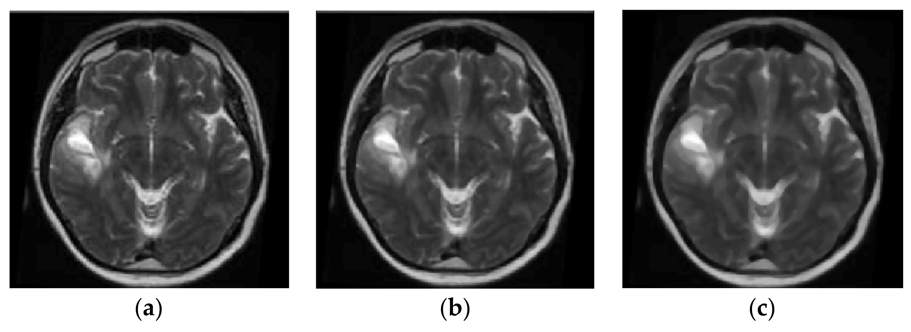
Figure 6.
The original image with moles and gray levels between 80 and 182 (a) and the normalized image in the full gray level range (0, 255) (b).
Figure 6.
The original image with moles and gray levels between 80 and 182 (a) and the normalized image in the full gray level range (0, 255) (b).

Figure 7.
Gradient operation voting one of the operational bins [15].
Figure 7.
Gradient operation voting one of the operational bins [15].

Figure 8.
Classification with k-NN using the features (f2, f3). Citrus disease (a) and skin disorders (b).
Figure 8.
Classification with k-NN using the features (f2, f3). Citrus disease (a) and skin disorders (b).

Figure 9.
Classifying 20, (f1, f2) pairs in four clusters corresponding to the skin disorders: acne (X mark), mycosis (round marks), papillomas (square marks), and vitiligo (pyramids).
Figure 9.
Classifying 20, (f1, f2) pairs in four clusters corresponding to the skin disorders: acne (X mark), mycosis (round marks), papillomas (square marks), and vitiligo (pyramids).

Figure 10.
Classification with SVM using the features (f2, f3) in citrus deficiency (a) and mycosis (b).
Figure 10.
Classification with SVM using the features (f2, f3) in citrus deficiency (a) and mycosis (b).

Figure 11.
Classification with a decision tree (a) using the features (f2, f3) of skin disorder (b).
Figure 11.
Classification with a decision tree (a) using the features (f2, f3) of skin disorder (b).

Figure 12.
The reference negative/positive samples (a) are recognized as TN, TP, FP, FN (b).


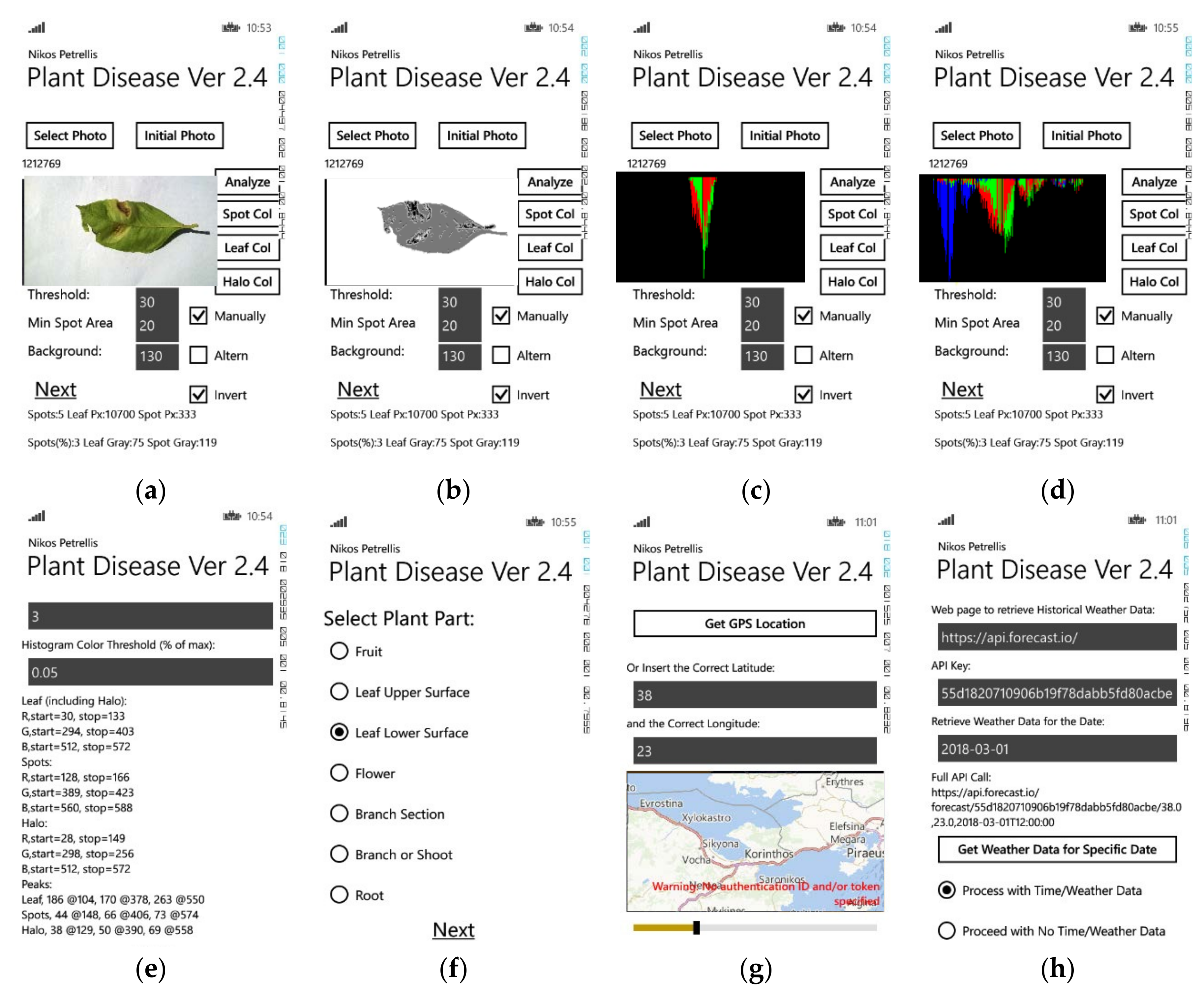
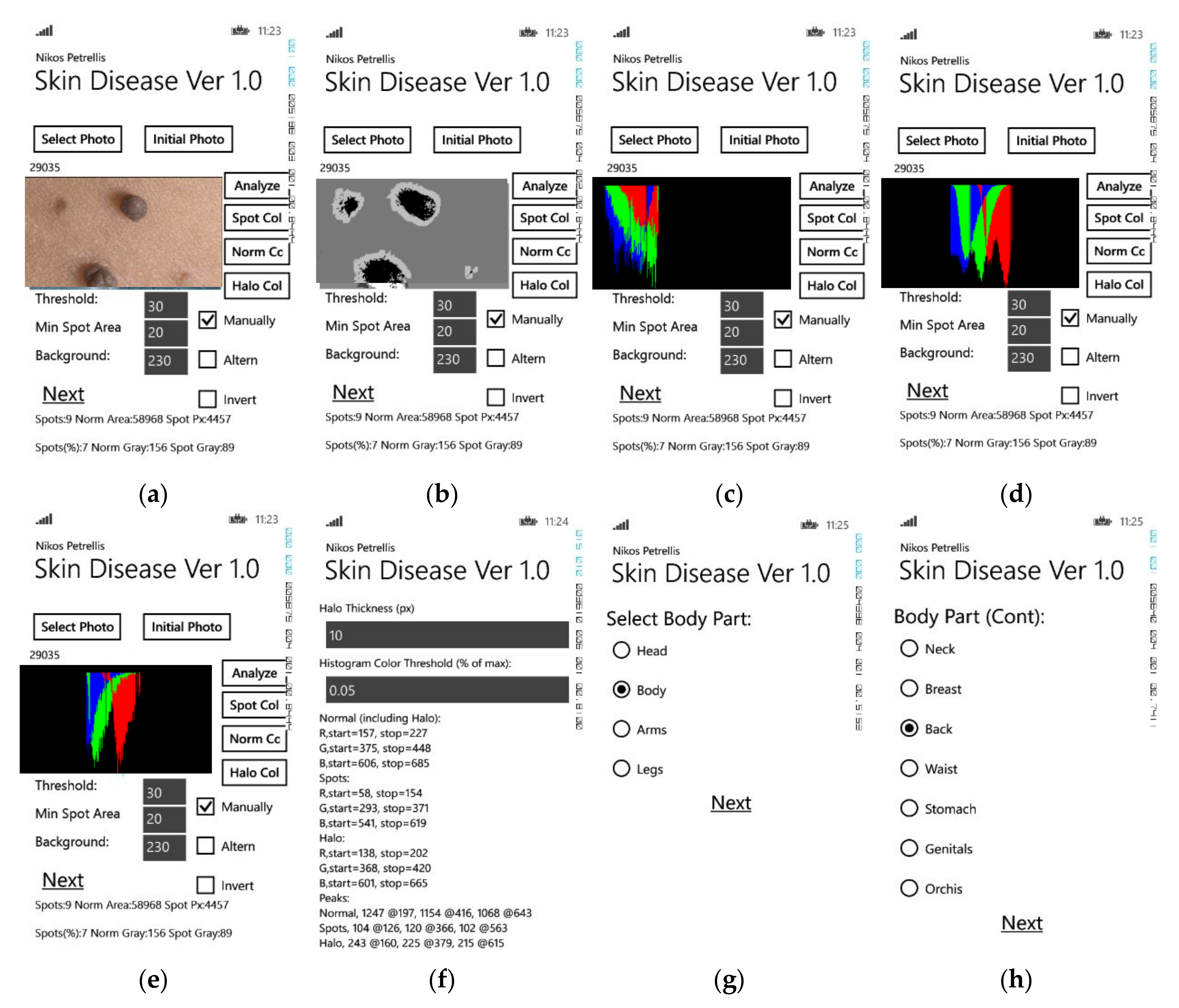
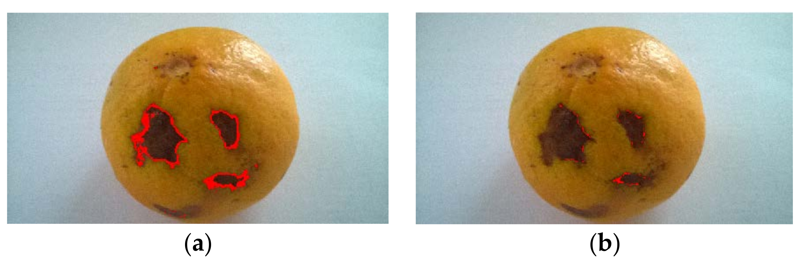
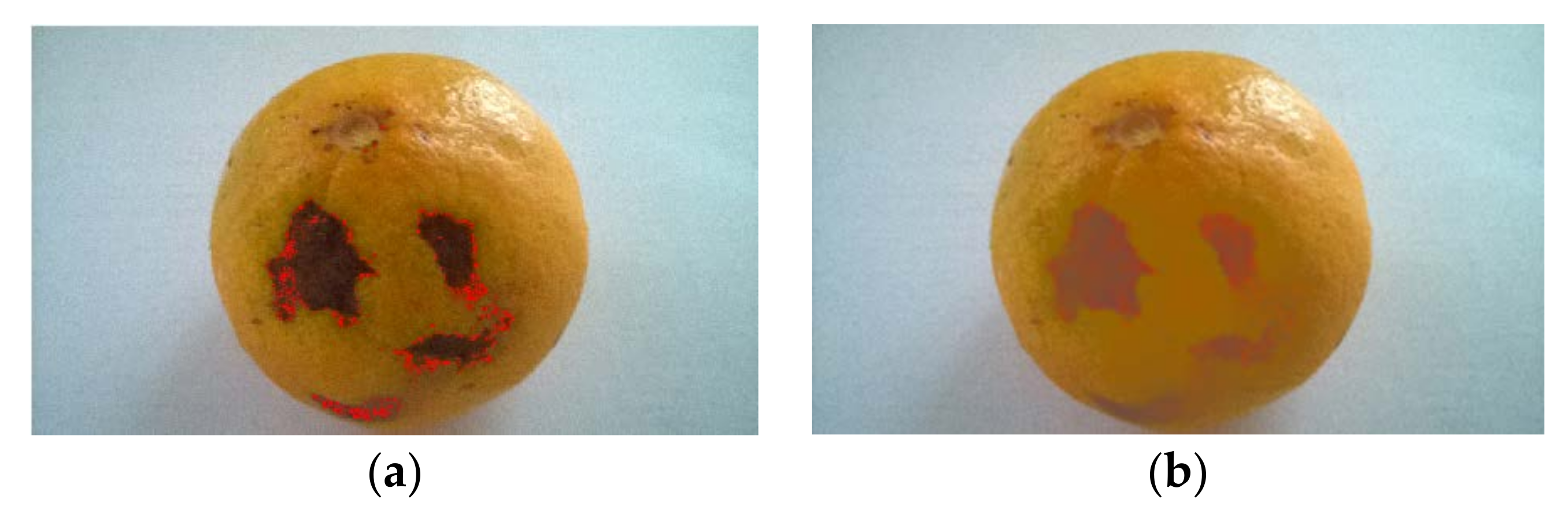
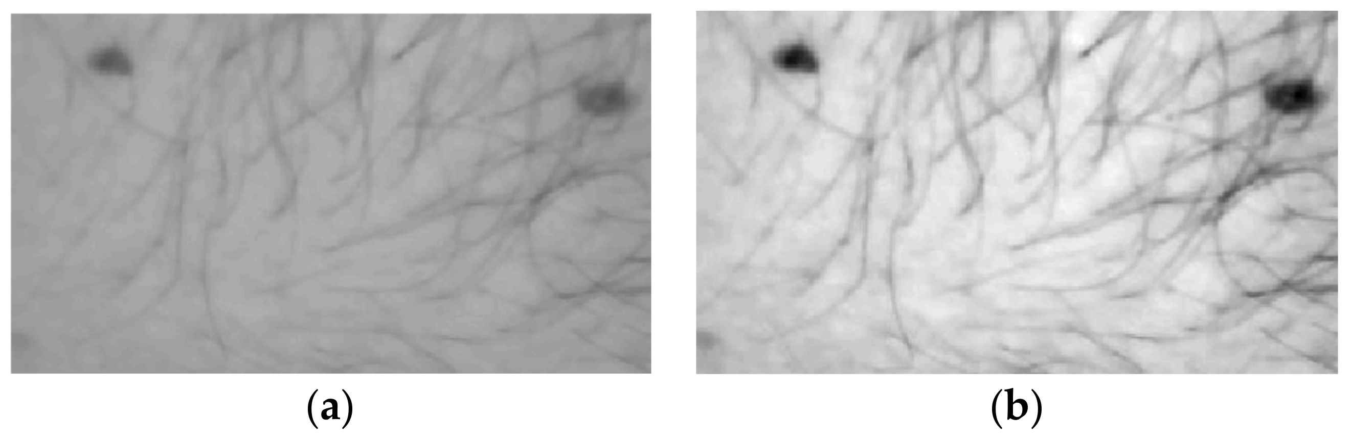
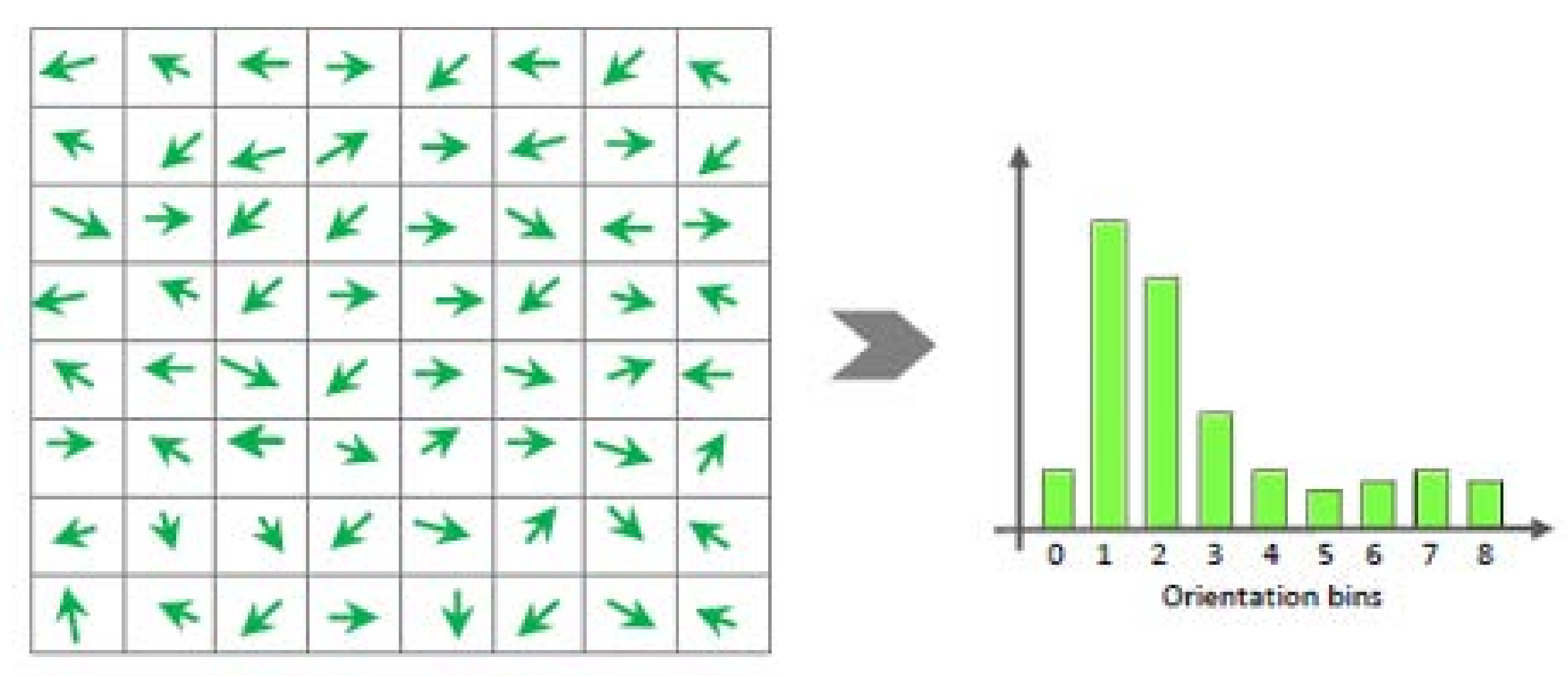
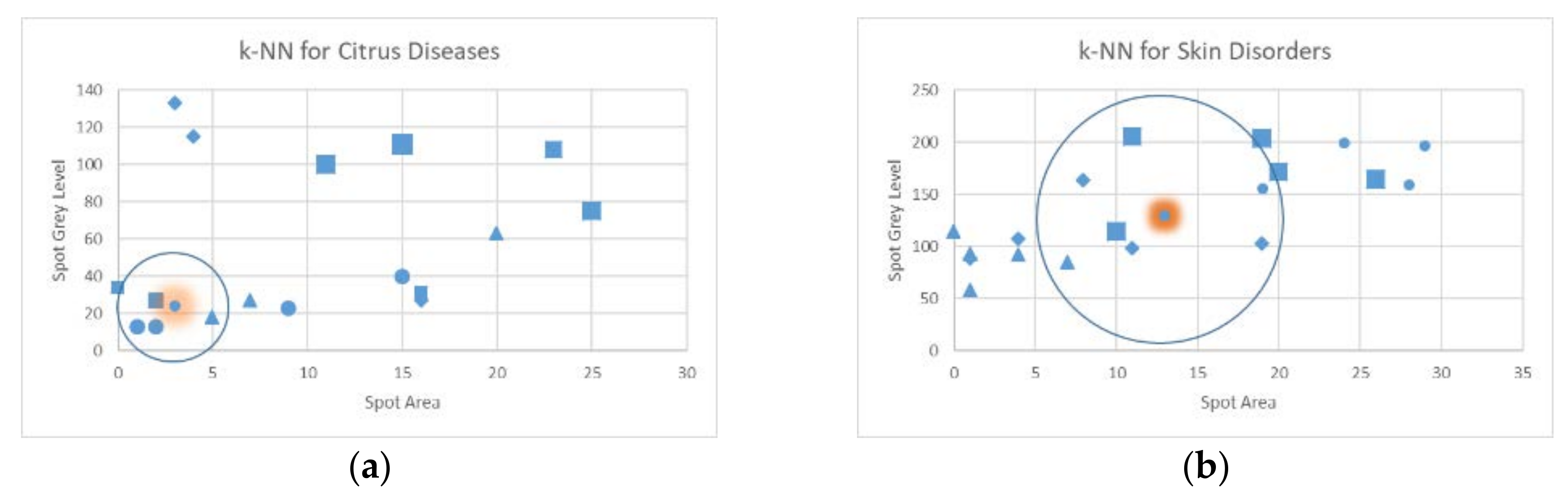
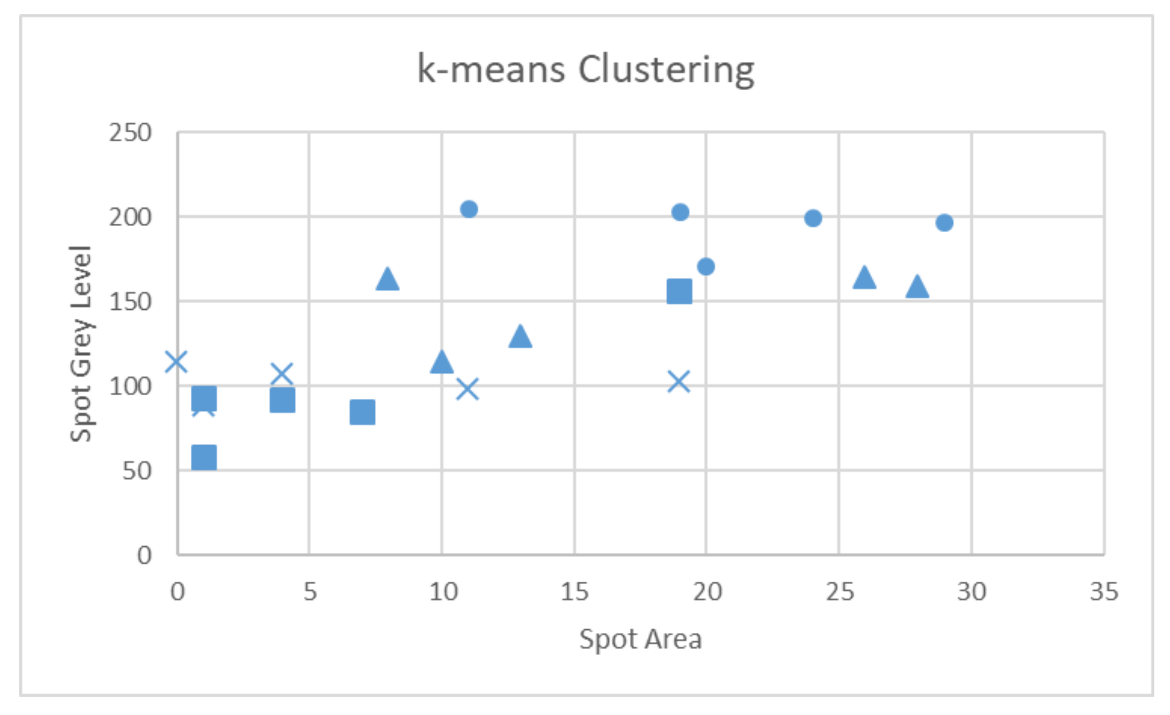
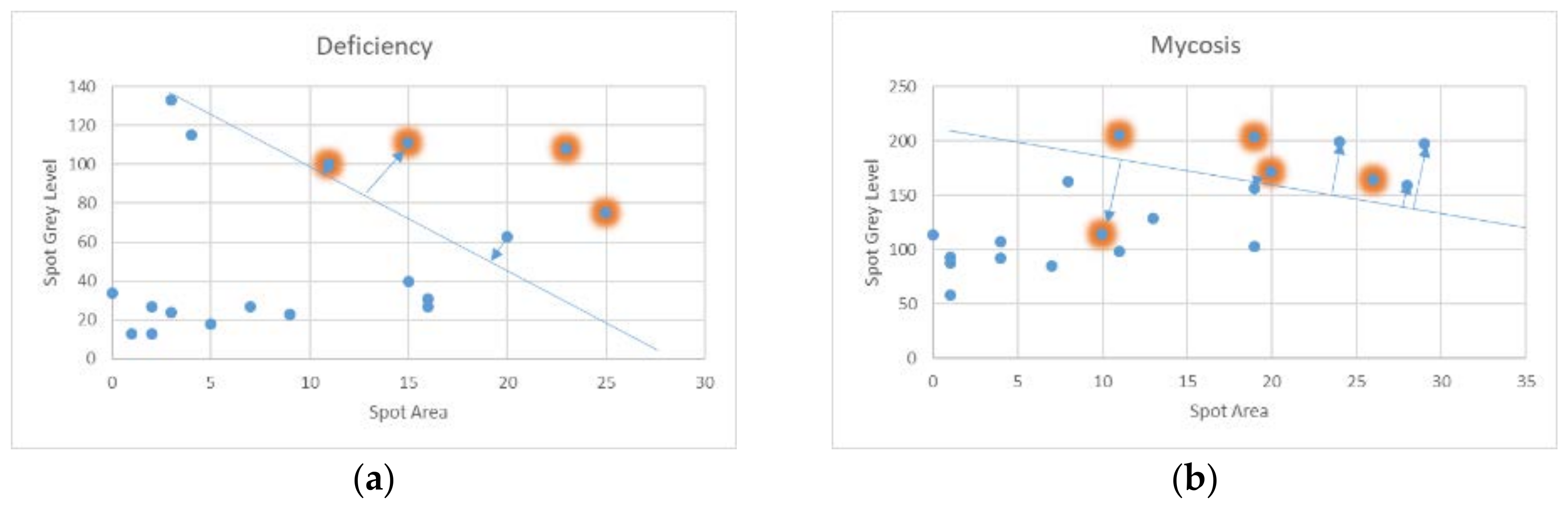
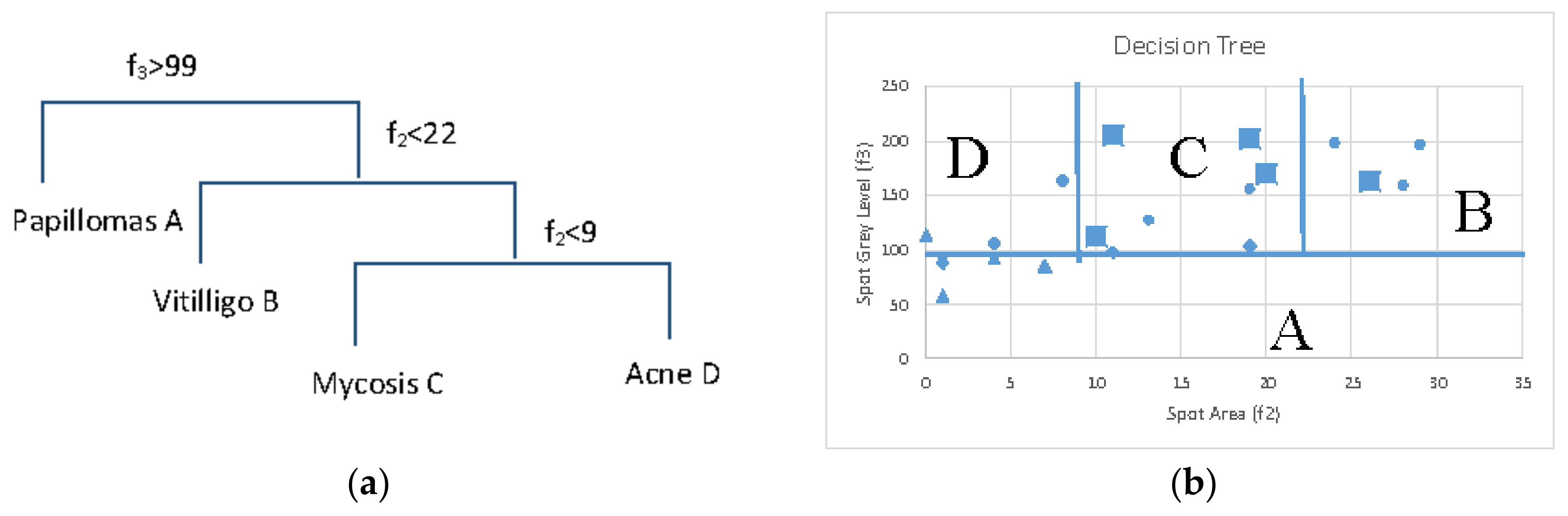
Table 1.
The features used in the Plant and Skin Disease applications.
| Feature (fi) | Plant Disease [71,72] | Skin Disease [40] |
|---|---|---|
| Number of spots (f1) | Yes | Yes |
| Spot area (f2) | Yes | Yes |
| Gray level of normal part (f3) | Yes | No |
| Gray level of spots (f4) | Yes | Yes |
| Gray level of halo (f5) | No | No |
| Histogram features (f6–f32) | Spots, Normal, Halo | Spots, Halo |
| (begin, peak, end) | ||
| Body or plant part (f33) | Yes | Yes |
| Temperature (f34, f35) | Yes | No |
| Humidity (f36) | Yes | No |
Table 2.
Example training samples for citrus diseases.
| Citrus Disease: | Spots (f1) | Relative Area (f2) | Gray Level of Spots (f4) | Histogram SR Begin (f6) | Histogram SR Peak (f7) | Histogram SR End (f8) |
|---|---|---|---|---|---|---|
| Alternaria (C1) | 19 | 16 | 31 | 22 | 33 | 43 |
| 2 | 0 | 34 | 28 | 34 | 43 | |
| 23 | 2 | 27 | 15 | 20 | 69 | |
| Mean | 14.66 | 6 | 30.66 | 21.66 | 29 | 51.66 |
| Std Deviation | 11.15 | 7.72 | 3.51 | 6.5 | 7.81 | 15 |
| CCDV (C2) | 3 | 1 | 13 | 0 | 14 | 17 |
| 4 | 2 | 13 | 4 | 10 | 18 | |
| 5 | 9 | 23 | 7 | 21 | 36 | |
| 5 | 3 | 24 | 14 | 27 | 37 | |
| Mean | 4.25 | 3.75 | 18.25 | 6.25 | 18 | 27 |
| Std Deviation | 0.95 | 3.6 | 6.07 | 5.91 | 7.53 | 10.98 |
| Deficiency (C3) | 11 | 11 | 100 | 87 | 110 | 163 |
| 11 | 25 | 75 | 61 | 78 | 124 | |
| 9 | 23 | 108 | 103 | 138 | 164 | |
| 10 | 15 | 111 | 106 | 123 | 183 | |
| Mean | 10.25 | 18.5 | 98.5 | 89.25 | 112.25 | 158.5 |
| Std Deviation | 0.95 | 6.61 | 16.34 | 20.6 | 25.54 | 24.77 |
| Anthracnose (C4) | 16 | 16 | 27 | 11 | 29 | 50 |
| 12 | 4 | 115 | 90 | 118 | 157 | |
| 16 | 3 | 133 | 142 | 161 | 189 | |
| Mean | 14.66 | 7.66 | 91.66 | 81 | 102.66 | 132 |
| Std Deviation | 2.31 | 7.23 | 56.72 | 65.96 | 67.32 | 72.79 |
| Melanose (C5) | 94 | 7 | 27 | 11 | 41 | 47 |
| 44 | 5 | 18 | 9 | 26 | 42 | |
| 10 | 20 | 63 | 40 | 81 | 111 | |
| 116 | 15 | 40 | 25 | 62 | 73 | |
| Mean | 66 | 11.75 | 37 | 21.25 | 52.5 | 68.25 |
| Std Deviation | 47.97 | 6.99 | 19.54 | 14.38 | 24 | 31.57 |
Table 3.
Example training samples for skin disorders.
| Skin Disorder: | Spots (f1) | Relative Area (f2) | Gray level of spots (f4) | Histogram SR begin (f6) | Histogram SR peak (f7) | Histogram SR end (f8) |
|---|---|---|---|---|---|---|
| Vitiligo | 17 | 24 | 199 | 199 | 205 | 240 |
| 34 | 19 | 156 | 177 | 186 | 198 | |
| 16 | 13 | 129 | 145 | 168 | 181 | |
| 14 | 28 | 159 | 175 | 181 | 198 | |
| 22 | 29 | 197 | 210 | 229 | 250 | |
| Mean | 20.6 | 22.6 | 168 | 181.2 | 193.8 | 213.4 |
| Std Deviation | 8.05 | 6.65 | 29.78 | 25.06 | 23.74 | 29.88 |
| Acne | 61 | 19 | 103 | 0 | 136 | 196 |
| 26 | 1 | 88 | 67 | 158 | 168 | |
| 23 | 4 | 107 | 100 | 173 | 179 | |
| 8 | 11 | 98 | 21 | 167 | 197 | |
| 22 | 8 | 163 | 175 | 208 | 219 | |
| Mean | 28 | 8.6 | 111.8 | 72.6 | 168.4 | 191.8 |
| Std Deviation | 19.71 | 6.95 | 29.49 | 69.28 | 26.21 | 19.46 |
| Papillomas | 15 | 1 | 93 | 138 | 149 | 194 |
| 4 | 1 | 58 | 46 | 102 | 108 | |
| 3 | 0 | 114 | 142 | 148 | 161 | |
| 16 | 7 | 85 | 121 | 142 | 171 | |
| 8 | 4 | 92 | 109 | 134 | 148 | |
| Mean | 9.2 | 2.6 | 88.4 | 111.2 | 135 | 156.4 |
| Std Deviation | 6.06 | 2.88 | 20.15 | 38.79 | 19.39 | 31.86 |
| Mycosis | 98 | 11 | 205 | 190 | 206 | 224 |
| 100 | 19 | 203 | 115 | 180 | 198 | |
| 274 | 26 | 164 | 112 | 147 | 189 | |
| 108 | 10 | 114 | 156 | 178 | 189 | |
| 184 | 20 | 171 | 177 | 188 | 199 | |
| Mean | 152.8 | 17.2 | 171.4 | 150 | 179.8 | 199.8 |
| Standard Deviation | 76.58 | 6.68 | 37 | 35.47 | 21.4 | 14.34 |
Table 4.
Estimated values of p(fi|Cq) for citrus diseases.
| Citrus Disease | f1 | f2 | f3 | f4 | f5 | f6 | Cest |
|---|---|---|---|---|---|---|---|
| Alternatia | 0.037 | 0.046 | 0.003 | 0.017 | 0.019 | 0.020 | 7.6 × 10⁻¹² |
| CCDV | 0.276 | 0.114 | 0.016 | 0.012 | 0.016 | 0.020 | 4.3 × 10⁻¹⁰ |
| Deficiency | 7.302 | 0.072 | 0.023 | 0.018 | 0.015 | 0.016 | 1.1 × 10⁻⁸ |
| Anthracnose | 0.427 | 0.057 | 0.007 | 0.006 | 0.006 | 0.005 | 6.7 × 10⁻¹² |
| Melanose | 0.008 | 0.062 | 0.018 | 0.021 | 0.015 | 0.012 | 7.6 × 10⁻¹² |
Table 5.
Estimated values of p(fi|Cq) for skin disorder.
| Citrus Disease | f1 | f2 | f3 | f4 | f5 | f6 | Cest |
|---|---|---|---|---|---|---|---|
| Vitiligo | 0.056 | 0.074 | 0.013 | 0.016 | 0.017 | 0.013 | 3.8 × 10⁻¹¹ |
| Acne | 0.02 | 0.06 | 0.013 | 0.006 | 0.015 | 0.019 | 5.4 × 10⁻¹² |
| Papillomas | 0.07 | 0.135 | 0.017 | 0.01 | 0.019 | 0.012 | 7.5 × 10⁻¹¹ |
| Mycosis | 0.005 | 0.07 | 0.01 | 0.011 | 0.018 | 0.026 | 4.2 × 10⁻¹² |
Table 6.
Comparison of skin disorder diagnosis referenced approaches.
| Ref | Disorder | Method | Accuracy (%) | Sens (%) | Spec (%) |
|---|---|---|---|---|---|
| [32] | Melanoma, Psoriasis, Dermo | AdaBoost classification framework | 90 | ||
| [21] | Eczema/Acne/ | Feedforward Back propagation ANN | 88/85/ | ||
| Leprosy/Psoriasis/ | 89/91/ | ||||
| Scabies/Foot Ulcer/ | 89/97/ | ||||
| Vitiligo/T. Corporis/ | 97/86/ | ||||
| Rosea | 89 | ||||
| [29] | Psoriasis | Back propagation NN Auto-associative NN | 70–90 | ||
| 40–80 | |||||
| [30] | Eczema, Acne, Leprosy, Benign, Dandruff, Syringoma, Mastitis, Scabies, Vitiligo, Diapercandi | ANN | 90 | ||
| [31] | Acne | k-means (Segmenation) Acne/Inflamatory discrimination (SVM Or Fuzzy C-means) Acne/normal skin discrimination with Fuzzy C-means | 70 | ||
| 66.6 | |||||
| 80 | |||||
| 100 | |||||
| [33] | Acne/Eczema | FFBP-NN | 97/88 | ||
| 89/88 | |||||
| Psoriasis/TineaCorporis Scabies/Vitiligo | 98/99 | ||||
| [34] | psoriasis, seboreic dermatitis, lichen planus, pityriasis rosea, cronic dermatitis and pityriasis rubra pilaris | BP-NN | 91 | ||
| [35] | leprosy, tineaversi color, vitiligo | SVM | 89.6 | ||
| [36] | Eczema, Impetigo, psoriasis | BP-NN | 80 | 71.4 | 87.5 |
| [38] | Psoriasis, Seborrheic Dermatitis, Lichen Planus, Pityriasis Rosea, Chronic Dermatitis (CD), Pityriasis Rubra Pilaris | ANN/Decision Trees/k-NN | 98/97/82, | ||
| 93/92/88, | |||||
| 97/95/87, | |||||
| 85/89/75, | |||||
| 92/91/83, | |||||
| 95/97/- | |||||
| [40] | Acne/Melanoma/Mycosis/Papillomas/Psoriasis/Vitiligo/Warts | Fuzzy Clustering | 100/73/78/52/46/95/39 |
Table 7.
Comparison of melanoma diagnosis approaches.
| Ref | Method | Accur (or JI) (%) | Sens (%) | Spec (%) | FPR (%) | BCR (%) | Error |
|---|---|---|---|---|---|---|---|
| [14] | Fuzzy clustering (α = 0.08) | 92.6 | 13.5 | ||||
| [15] | SVM | 97.3 | 98.2 | 96.4 | |||
| [16] | Level Set (Otsu) | 95 | 98 | 90 | 93 | 5.7 | |
| Global AC (Otsu) | 94 | 98 | 89 | 91 | 6 | ||
| Local AC (Otsu) | 95 | 98 | 90 | 91 | 5.8 | ||
| Level Set(Kapur) | 96 | 98 | 91 | 93 | 5 | ||
| GlobalAC Kapur) | 96 | 98 | 90 | 92 | 5.9 | ||
| Local AC (Kapur) | 95 | 98 | 90 | 92 | 5.7 | ||
| [17] | 97 | 100 | 95 | ||||
| [18] | MLP | 92 | 92.3 | 91.6 | |||
| [20] | NN | 10−6 (SSE) | |||||
| [22] | SVM | 80.7 | 85.6 | 9.7 | |||
| [23] | SVM | 93.5 | 95 | 92 | |||
| [24] | Multilevel thresholding | 96.8 | 99.9 | 95.2 |
Table 8.
Comparison of MRI-based approaches.
| Ref | Disease | Method | DSC (%) | Accur (or JI) (%) | Sens (%) | Spec (%) | FPR (%) | FNR (%) | MAD | MaxD |
|---|---|---|---|---|---|---|---|---|---|---|
| [6] | Alzheimer’s | SVM | 29 | 99.7 | 98.9 | 53.7 | ||||
| RF | 32.8 | 99.8 | 98.6 | 73.6 | ||||||
| DBM | 68 | 99.6 | 99.7 | 35.8 | ||||||
| CEN | 42.4 | 99.7 | 42.4 | 99.7 | ||||||
| Patch-CNN | 53.7 | 99.7 | 99.8 | 53.8 | ||||||
| [7] | Brain tumor | DWT + PCA + RF | 95.7 | |||||||
| [8] | Brain tumor | ACWE (3D) | 89 | 99.9, 91(JI) | ||||||
| [52] | Prostate gland | Fuzzy-C from Multi-spectral | 91 | 84 (JI) | 89 | 99.9 | 0.15 | 6.9 | 2.7 | 8.5 |
| T2w | 81.9 | 71(JI) | 82.2 | 99.6 | 0.37 | 12.6 | 4.9 | 13.8 | ||
| T1w | 82.5 | 71 (JI) | 93.2 | 98.8 | 0.15 | 3.6 | 5.5 | 14.3 |
Table 9.
Comparison of other human disease diagnosis approaches.
| Ref | Disease | Method | Accur (%) | Sens (%) | Spec (%) |
|---|---|---|---|---|---|
| [41] | Breast Malign., Breast Benign | CNN | 91 | 93 | 82.5 |
| CNN | 93 | 91.5 | 84 | ||
| [42] | Breast Malignant | EM | 80 | ||
| Breast Benign | 82 | ||||
| [45] | Breast masses | SVM | 85 | ||
| [47] | Cardiovascular diseases | MLP | 86.2 | ||
| SVM | 89.5 | ||||
| Bayes | 79.6 | ||||
| [49] | Retinal vessels | CNN | >90 | ||
| [53] | Liver fat | Threshold-based | 79–98.8 | 87–100 |
Table 10.
Comparison of precision agriculture applications.
| Ref | Application | Method | Succ.Rate(%) | Sens (%) | Error |
|---|---|---|---|---|---|
| [68] | Seedling counting | Otsu thresholding | 89.9–99.2 | ||
| [73] | Fruit count | Naïve Bayes/Decision Tree/RF/ANN/SVM | 48/79/79/85/85 | ||
| [74] | Fruit pregrading | Size/CCI classification of maturity | |||
| Category 1 | 100/84 | 0/16 | |||
| Category 2 | 100/90.7 | 0/9.3 | |||
| Category 3 | 100/98.1 | 0/1.9 | |||
| [75] | Pineapples/bittermelon counting | SVM | 68–85/91–100 | ||
| [76] | Fruit count | k-NN, SVM | 4–23 (RMSE) | 30–83 | 1–34 |
Table 11.
Comparison of plant disease diagnosis applications.
| Ref | Plant | Disease | Method | Accur (%) | Sens (%) | Error |
|---|---|---|---|---|---|---|
| [59] | Biotic stress | NN | 95–99 | |||
| [56] | Biotic stress | SVM/ANN | 69/58 | |||
| [62] | Citrus | Huanglongbing (HLB) | SVM | 90 | ||
| [66] | Citrus | HLB | SVT | 95–100 | ||
| [67] | Sugar beans | Cercospora | Spectral Angle Mapper (SAM) | 98 | ||
| SVM | 97 | |||||
| Powerdery Mildew | SAM | 62 | ||||
| Rust | SAM | 10 | ||||
| Headblight | SAM | 13 | ||||
| Infected tissues | CFI | 29 | ||||
| Healthy leaves | SAM/CFI combined | <5 | ||||
| [71] | Grape | Downy mildew | Fuzzy Clustering | 70–90 | ||
| Powdery mildew | 70–95 | |||||
| Pierce | 85–90 | |||||
| Esca | 90–95 |
© 2018 by the author. Licensee MDPI, Basel, Switzerland. This article is an open access article distributed under the terms and conditions of the Creative Commons Attribution (CC BY) license (http://creativecommons.org/licenses/by/4.0/).
Share and Cite
MDPI and ACS Style
Petrellis, N. A Review of Image Processing Techniques Common in Human and Plant Disease Diagnosis. Symmetry 2018, 10, 270. https://doi.org/10.3390/sym10070270
AMA Style
Petrellis N. A Review of Image Processing Techniques Common in Human and Plant Disease Diagnosis. Symmetry. 2018; 10(7):270. https://doi.org/10.3390/sym10070270
Chicago/Turabian StylePetrellis, Nikos. 2018. "A Review of Image Processing Techniques Common in Human and Plant Disease Diagnosis" Symmetry 10, no. 7: 270. https://doi.org/10.3390/sym10070270
Note that from the first issue of 2016, this journal uses article numbers instead of page numbers. See further details here.