Vortex Creation without Stirring in Coupled Ring Resonators with Gain and Loss
by
 , and
, and
Aleksandr Ramaniuk
1,* ,
,
Nguyen Viet Hung
2,
Michael Giersig
3,4,
Krzysztof Kempa
5,
Vladimir V. Konotop
6 and
Marek Trippenbach
1 1
Faculty of Physics, University of Warsaw, ul. Pasteura 5, PL-02-093 Warszawa, Poland
2
Advanced Institute for Science and Technology, Hanoi University of Science and Technology, 100803 Hanoi, Vietnam
3
Department of Physics, Freie Universität Berlin, Arnimalle 14, D-14195 Berlin, Germany
4
International Academy of Optoelectronics at Zhaoqing, South China Normal University, 526238 Guangdong, China
5
Department of Physics, Boston College, Chestnut Hill, MA 02467, USA
6
Centro de Física Teórica e Computacional and Departamento de Física, Faculdade de Ciências, Universidade de Lisboa, Campo Grande, Edifício C8, 1749-016 Lisboa, Portugal
*
Author to whom correspondence should be addressed.
Symmetry 2018, 10(6), 195; https://doi.org/10.3390/sym10060195
Submission received: 30 April 2018
/
Revised: 18 May 2018
/
Accepted: 28 May 2018
/
Published: 1 June 2018
(This article belongs to the Special Issue Broken Symmetry)
Abstract
:We present the study of the dynamics of a two-ring waveguide structure with space-dependent coupling, linear gain and nonlinear absorption; the system that can be implemented in polariton condensates, optical waveguides and nanocavities. We show that by turning on and off local coupling between rings, one can selectively generate a permanent vortex in one of the rings. We find that due to the modulation instability, it is also possible to observe several complex nonlinear phenomena, including spontaneous symmetry breaking, stable inhomogeneous states with an interesting structure of currents flowing between rings, the generation of stable symmetric and asymmetric circular flows with various vorticities, etc. The latter can be created in pairs (for relatively narrow coupling length) or as a single vortex in one of the channels, which later alternates between channels.
1. Introduction
Coupled microrings (microdisks, or more generally microcavities) are standard basic elements in diverse physical applications. In optics, they are used for nonreciprocal devices [1], switches [2], loss control of lasing [3] and ring lasers [4,5], to mention a few. Recently, the attention has also turned to more sophisticated devices, which include several coupled microcavities and which are referred to as photonic molecules [6]. Coupled non-Hermitian microcavities are also used for the study of chiral modes in exciton-polariton condensates [7], as well as for modeling coupled circular traps for Bose–Einstein condensates (BEC), where gain corresponds to adding atoms, while nonlinear losses occur due to inelastic two-body interactions. They can also be realized in nanoplasmonic systems [8] and slow-light optical microcavities [9].
Like in the case of any coupled subsystems, the characteristics of coupling between microrings (or to an external element, for instance, to a bus fiber) may strongly affect the stationary regimes, as well as the dynamics supported by the system. The coupling can be modified in various ways. It depends on the geometry (i.e., on the mutual locations of the rings), on the wave-guiding characteristics of the rings, which determine the field decay outside the cavities, on the medium between the cavities (it can be homogeneous or gradient; active, absorbing or conservative), etc. Thus, it is of natural interest to understand how the characteristics of coupling affect the field distribution and dynamics inside the ring cavities. This is the question that is addressed in the present work. The main emphasis is made on the interplay between the size of the coupling domain and other spatial scales of the system (i.e., on the ring lengths and on the characteristic scales of the excited modes).
Before we move on to a specific model (formulated in Section 2), the stationary solutions of which are investigated in Section 3, the dynamical regimes in Section 4 and Section 5 and vortices in Section 6, we would like to advertise our effort to design a nanostructure of coupled rings to explore experimentally this and similar settings and their dynamics. In Section 7, we discuss the specific experimental proposal based on the structures that were already manufactured.
2. The Model
In the present study, we consider a model described by two coupled nonlinear Schrödinger equations with gain and nonlinear loss (depending on the applications, they also can be termed Gross–Pitaevskii or Ginzburg–Landau equations), which we write down in scaled dimensionless units:
Here, and are the fields in the first and second waveguides, is the linear gain and is the nonlinear loss, both considered constants along the waveguides, and is the position depending coupling.
Extended discussion of the model (1) and of its applications can be found in a previous publication [10], where the rings were homogeneously coupled, i.e., where it was assumed that is constant. We also mentioned that (1) with constant coupling is analogous to the model introduced earlier in [11], where it was considered on the whole axis subject to the zero boundary conditions. In this paper, we focus on expanding the study of the model through introducing coupling modulation . We consider rings assuming, without loss of generality, that . This implies periodic boundary conditions for both channels: , and the coupling function is extended only in a certain region of the rings. In particular, for numerical simulations, we shall consider local Gaussian coupling in the following form:
where w is the width of the coupling, while characterizes the coupling strength. Our results are not sensitive to the particular shape of the wavefunction, as we have checked using super Gaussian functions with very high power.
An important remark about the terminology used is in order. For all applications mentioned in the Introduction, the meaning of the variable x is an angle defining a point on the circumference. The functions are rather envelopes of the field distributions rather than the total fields (see, e.g., [12] for optical resonators and [13,14] for BEC applications). Thus, solutions for having nonzero topological charge (see [10]) may correspond to the total field distributions having phase singularities in the centers of the rings. In other words, such solutions describe vortices. Taking this into account, the respective solutions are referred to below as vortices. System (1) is simple, but possesses a surprisingly rich and diverse set of stable states (some of them nonstationary). For the limit of very wide coupling (), we expect the same results dynamics as for the constant coupling (this is described in [10]). On the other side, very narrow coupling () allows approximating coupling with the delta function.
Most of the results found in the present study are numerical (using propagation techniques). In this context, there is one important issue that we need to address before we present the outcome of our investigations. As discussed in [10], for the uncoupled case (), one can find stable background solutions in the form:
Once the rings become coupled, modulation instability occurs mostly due to the interplay between gain and nonlinear absorption. In the case of constant coupling in [10], two distinct classes of solutions have been found analytically: symmetric, characterized by , and anti-symmetric with . The anti-symmetric solutions are always stable, and symmetric ones are usually unstable. Therefore, we decided to perform numerical studies using the symmetric state as the initial condition. This led us to a plethora of new states and attractors [10].
We found that even if the coupling is not uniform, the dynamics starting from anti-symmetric states leads to an anti-symmetric stationary stable solution (see the examples of such attractors in Figure 1). On the other hand, starting from a symmetric state, in some regions of parameters, does not necessarily lead to the antisymmetric stationary states, but can traverse to the more interesting attractors, like limit cycles or even chaotic states. Hence, below, we focus on the dynamics starting with the symmetric initial state with small perturbation imposed in the form of:
where the perturbation was typically of the order of . In our simulations, we took the value of the gain parameter larger than loss , and we checked that all results are qualitatively the same, regardless of the particular values of these parameters. The results also do not depend on particular values of the amplitude of the perturbation or perturbation wavenumber k. In the case of stronger loss (), results seem to be different, and they are not included here. In this article, we assume for all later considerations and propagate from the initial state defined with (4), unless stated otherwise. All simulations were performed via the split-step Fourier method [15].
3. Stationary Solutions
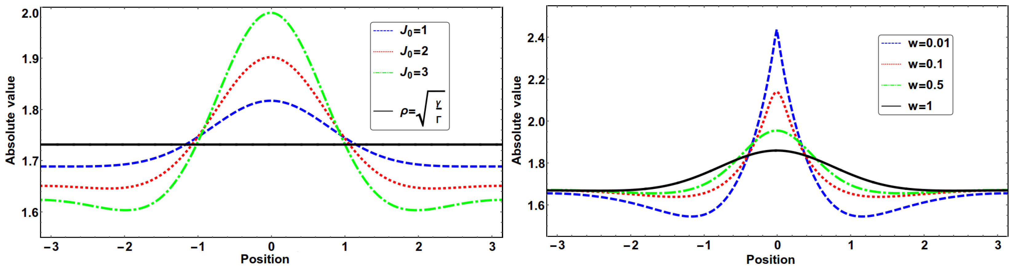
When the coupling between the rings is weak (), starting from the initial state (4), we observed that the propagation leads to stable, stationary anti-symmetric solutions. The resulting wavefunction has the form of a constant background with the bulge in the coupling region, which depends on coupling function , as presented in Figure 1. In this figure, we plot the modulus of the wavefunction for unitary width () and various coupling constants (Figure 1 left panel). In the right panel of Figure 1, we fix and change w, going towards narrow distributions, to show what one can expect when the coupling has the form of the Dirac delta function. We also show the background level, plotting it as a black horizontal reference line, in the left panel of Figure 1.
In order to interpret the results of Figure 1, we first notice that for antisymmetric solutions , the coupling plays the role of the linear potential well, , thus leading to the equation:
Let us now rewrite this model in the hydrodynamic form, introducing the amplitude distribution , as well as the phase gradient , through the relation . For the stationary solution, we obtain from (5):
Due to the parity symmetry of the problem and taking into account the continuity of the solution (i.e., of the functions and and of their derivatives), we have the relations:
Now, we observe that the maximal density is achieved at , i.e., at the point of the minimum of the potential energy landscape . Thus, at , we obtain from (6) that , and thus, , meaning that the energy flow is directed towards the minimum of the effective potential (which is expected):
Similarly, one can analyze the point , located at the opposite side of the ring diameter. Denoting , we have . Now, , and thus, . This is what we observe in both panels of Figure 1. In particular, in the left panel of Figure 1, we observe the decrease of with the increase of .
An interesting feature in the density distributions shown in both panels of Figure 1 is the appearance of the non-monotonic dependence of in the intervals and . In particular, the minimal density is achieved in two symmetric points of the ring, different from . As follows from (6), at these points, the absolute value of the velocity gradient is maximal. Since the solution separating monotonic and non-monotonic densities (in the intervals and ) is characterized by (at this solution, the curvature of changes its sign), it is not difficult to make an estimate of the parameters for that solution in the case of sufficiently narrow coupling. Indeed, in that case, and become negligibly small, and one obtains from (6) and (7) .
In the following subsections, we present the results of our studies of the dynamics of our system with increasing coupling strength. We shall distinguish two separate regimes of very narrow () and extended () couplings. As we shall see in these limiting cases, the dynamics can be of a quite different character.
4. Narrow Coupling Dynamics
In this section, we present the results obtained in simulations with a very narrow coupling function , where we used the Gaussian (2) of a width equal to . Our results are summarized in Figure 2, Figure 3 and Figure 4. They are also described in concise form below.
Depending on the value of , we can distinguish several different patterns characteristic for the long (asymptotic) regular behavior. It can be stationary or periodic. In all simulations, the system reaches the respective attractor state after a transient period, which depends on initial conditions and perturbation, and typically does not exceed in our arbitrary units.
For small coupling , asymptotically long time dynamics lead to a stable anti-symmetric state, shown with the black curve in Figure 2. This state exhibits a non-trivial phase structure, which is formed as a result of the non-Hermiticity of our model.
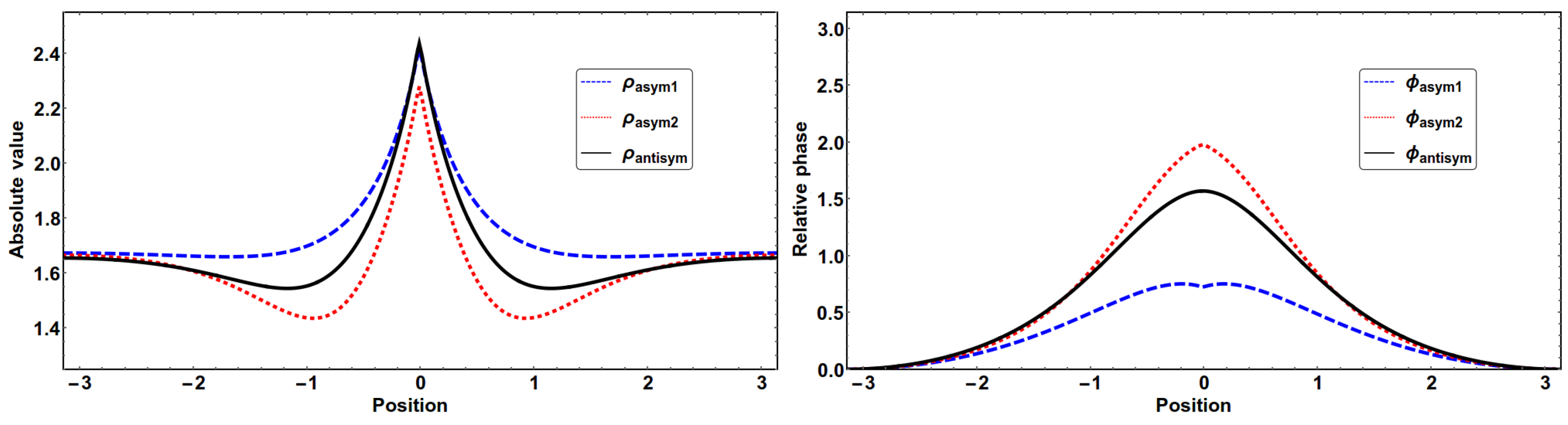
For slightly larger coupling , when we propagate initial symmetric distribution for as long as it takes to reach the steady state, we observe symmetry breaking (between channels), and our system approaches a stable asymmetric state, represented by blue () and red () curves in Figure 2. We observe that local minima of the densities are achieved at for the first ring and for intermediate points where for the second ring. To make a plot of the phase, we excluded an x-independent component of the phase linearly growing in time. Note that the hydrodynamic formulation allows us to discuss energy flow in the system. An interesting observation is that in the center of the coupling, i.e., in the vicinity , the energy flows in the two rings have opposite directions. Indeed, these flows are determined by , and in the vicinity in the first ring with higher field density, the current is directed outwards from the center (), while in the second ring, it is directed towards the center ().
Finally, for larger coupling , our system tends to the limit cycle dynamics, and we observe oscillations symmetric with respect to the center of the coupling region. It is an interesting class of solutions, and analogous dynamics was found in the broad coupling regime (see the next section). It seems to be universal, and the general picture of the dynamics in this regime does not depend on the width of the coupling. Due to this universality, we decided to discuss this class of solutions only for the broad coupling in the next section.
5. Broad Coupling Dynamics
In the opposite limit, when the range of the coupling is comparable to the length of the ring (but not uniform yet), we also observe a few classes of characteristic steady state dynamics, and we classify them according to the (increasing) value of coupling strength . We present results for and show asymptotic (in time) dynamics. In this case, since the most interesting steady state exhibits rather complex oscillations, corresponding to the limit cycle, we choose to present contour plots (see Figure 3) and dynamical snapshots at various times in Figure 4 and Figure 5. Animations of both oscillatory solutions are additionally presented in supplementary materials. Note that we always start from the perturbed symmetric state given in Equation (4), but our predictions are not sensitive to this particular choice.
As expected, the increase of the coupling strength leads to the increase of the oscillation frequency. An interesting observation, however, is that the transient period, i.e., the time necessary for establishing oscillations, also increases with . The oscillatory dynamics is symmetric with respect to both rings, with alternating field characteristics (amplitude and relative phase) exchanging after each half-period.
In the case of small coupling strength (), the dynamics lead directly to the anti-symmetric state, analogous to the one presented in Figure 2. This part is identical in both cases of broad and narrow coupling.
We did not find any asymmetric stationary states in the case of broad coupling. This class of states was only present for very narrow coupling, as mentioned above. Instead, we observe directly the transition to the next phase described below, namely symmetrically-oscillating states. However, in the broad coupling case, this is not the last category identified in our research. Above this class, as we describe below, there is an extra region of the most interesting solutions, where vortices are produced in an alternating manner, in one or the other channel.
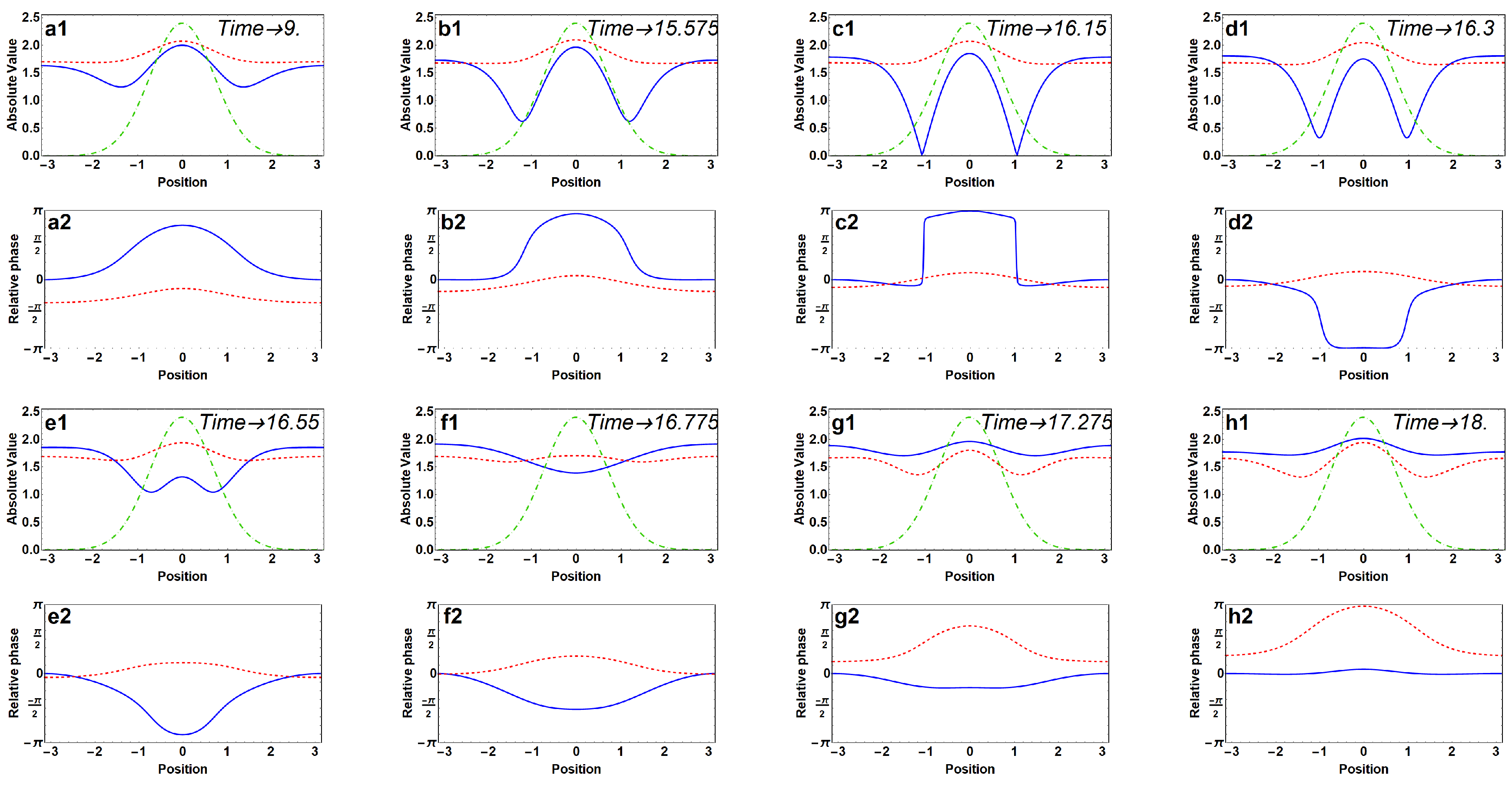
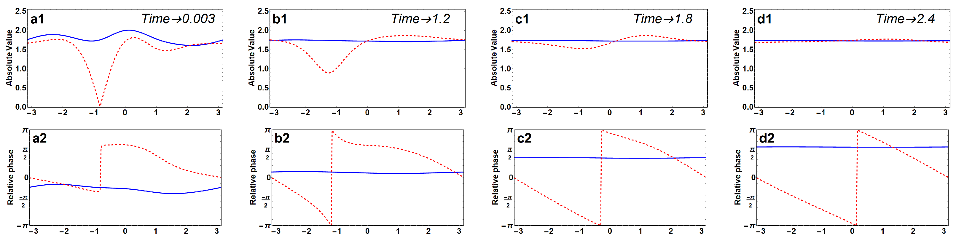
Upon increasing the value of coupling strength, at approximately , symmetric (with respect to the center of the Gaussian coupling function (2)) oscillations begin to develop, initially with a very long period, which becomes shorter at higher coupling strength. Details of the oscillations can be identified in Figure 3 and Figure 4. In the first figure, we now focus on the left panel (moving from the top to the bottom). First, the contour plot of the time evolution of the amplitude and phase oscillations of is shown (the wavefunction in the second channel is just shifted by a half period); next, we present the evolution of the norm in each channel () as a function of time, and finally, we present more details, the evolution of the norm of each of the wavefunctions and the average within the full period of oscillations. These results are complemented by the full view of the wavefunction during its half-period oscillations in the asymptotic regime in Figure 4. The first and the third rows show the modulus of the wavefunctions (blue and red curves correspond to the first and second channels, correspondingly), and the second and fourth rows show the phase structure. We can trace the dynamics in which one of the channels develops two symmetric dips (see Figure 4(a1,b1)) that develop slowly, reach the bottom (c1) and eventually flatten to make the exchange with its partner from the second channel (see Frames (e1–h1)). In parallel, we show the phase structure (Frames (a2) though (h2)), and perhaps, the most prominent feature is the very steep phase profile in Frames (c2) and (d2). It happens exactly at the time when the two dip structures in one of the moduli (blue curve in (c1)) reach zero at the minimum. Notice that the solution stays symmetric all the time. This will no longer be true when we go to the higher coupling regime.
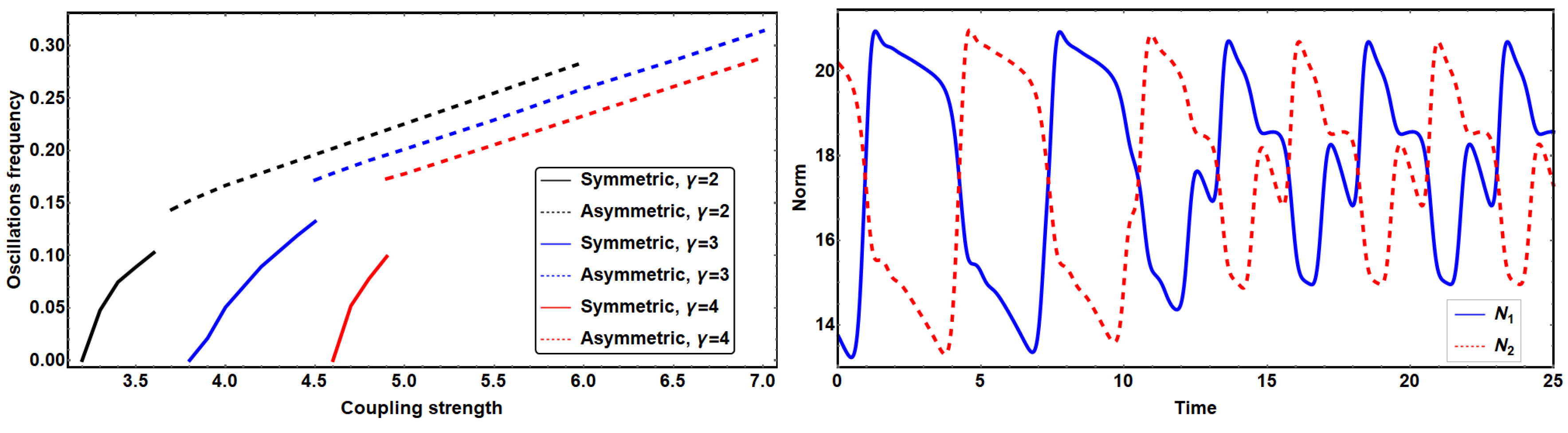
We investigated the frequency of oscillations of the periodic solutions. Results are presented in Figure 6. It is a collective plot containing the results not only for our central example of , but also two different values of this parameter (notice that we keep the value of ). At a small value of the coupling, frequency grows rapidly, then a sudden jump occurs, and further growth is linear. This jump is associated with yet another bifurcation (symmetry breaking), and as a matter of fact, solutions marked with dashed lines no longer belong to the class described above, as it exhibits asymmetric oscillations. We will describe it in more detail in the next section. In our leading example of , this phase transition occurs at coupling . In the transition region around this value of the coupling, we observe that the dynamics leads first to the symmetric oscillations, and after the transient period of several symmetric oscillations, it follows to the asymmetric oscillations, which are asymptotically stable. This transient behavior can be identified in the right panel of Figure 6, where we plot the norm of the wavefunctions. Additionally, animation of wavefunctions transition is presented in supplementary materials.
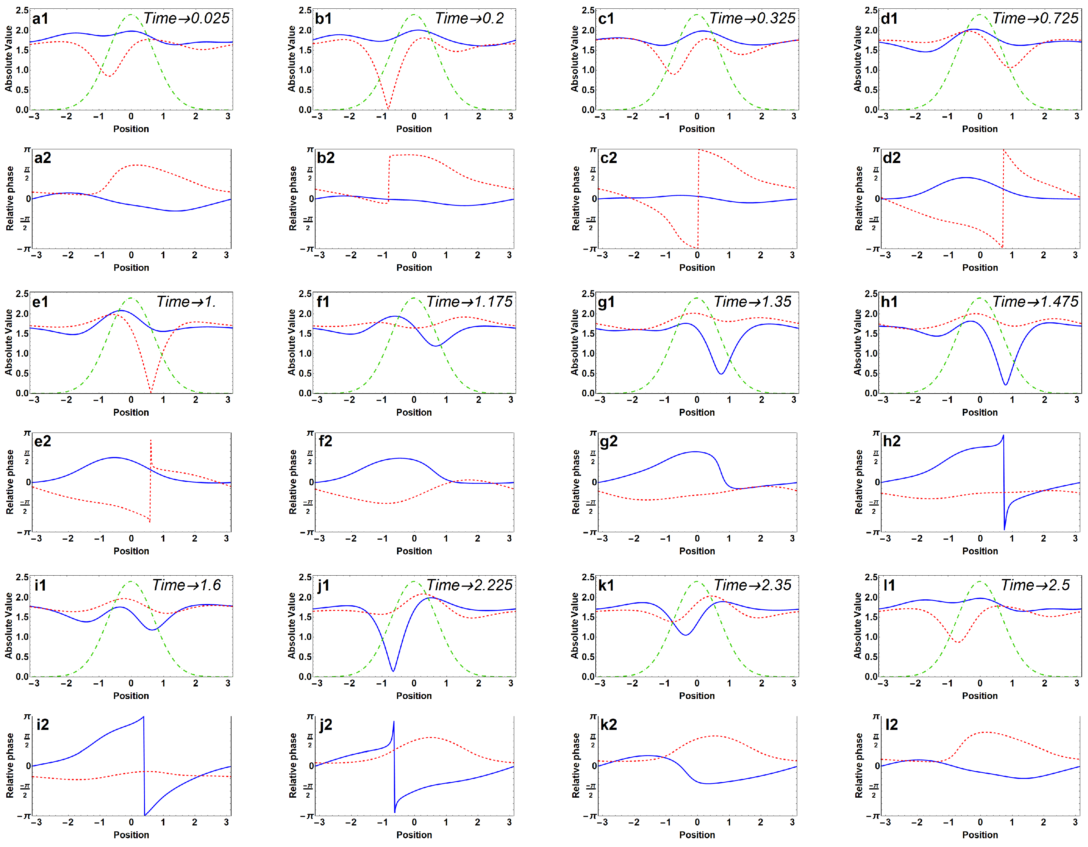
For values of the coupling above (this particular value corresponds to and ; see Figure 6), the phase structure becomes asymmetric with respect to the center of the coupling function; see Equation (2). This leads to the periodic, limited in time, appearance of a vortex in one of the channels, which then (on the regular basis) reappears in the opposite channel, with an inverted topological charge. The whole dynamics has again the form of regular oscillations, and we show various phases of the evolution of the wavefunctions in Figure 3 and Figure 5. In Figure 3, we show the time evolution of the modulus of the wavefunction and its phase on the contour plot. Note that in this regime, there is a single dip that appears once when a vortex is created (the vortex in our case, as we mentioned above, is equivalent to excitation) and again when the vortex disappears, only to show up a bit later in the opposite ring. One can follow this process even closer looking at Figure 5. In Panel (a1), we see the dip, which is just about to reach zero at around . The phase around this point is very steep (Panel (b)), and the vortex is created (there is a phase across the ring equal to ). Then, the wavefunction flattens, until the second dip starts to develop at around . Once the second dip reaches zero, the vortex disappears. Then, the whole process repeats itself in the second ring in reversed order (Panels (g)–(l)). This type of behavior was not observed in the case of narrow coupling, when we only have a symmetric structure. It seems that there is some distance between the edges of the coupling function necessary for this spacial symmetry to be broken.
6. On Vortex Creation without Stirring
Our system is non-Hermitian, and as such, it does not conserve topological charge; vortices can be created during the dynamics, even if the system is rotationally invariant. This happens due to the modulational instability, and as we mentioned above, in this 1D system, the vortex is equivalent to higher momentum excitations. Previously [10], for some values of the coupling constant, we demonstrated that the system can, starting from the perturbed symmetric state, arrive at the stationary states defined as:
Here, is an integer number expressing the value of the topological charge. This antisymmetric state is stable against initial perturbations. There is also a symmetric solution, where ; however, they are usually unstable, and we never observed that in the asymptotic limit of our simulations.
So far, we could create vortices with equal topological charges in both channels. However, here, when we define inhomogeneous local coupling, additionally varying in time (it is enough to switch it on for some time and then switch it off), there is even the more exciting possibility of creating the vortex only in one ring, accompanied by constant solution in the other. The idea is based on the results obtained for the broad coupling function, described in Section 5. Imagine that we start from the perturbed symmetric state (as we did in all the cases described in this manuscript) and we allow the system to evolve towards the regime of asymmetric oscillations. When the system is already in this regime, we will abruptly turn off the coupling between rings. The dynamics corresponding to this scenario is illustrated in Figure 7. Here, we present a series of snapshots of both wavefunctions and their phases. In Figure 5 in Panels (a1) and (b1), the coupling is still on, and one of the wavefunctions is at the stage when the vortex is created and the dip in the amplitude is fully developed (reaches the bottom). In the series of panels (columns) in Figure 7, the coupling between rings is off, and we observe slow, independent relaxation in each of them separately. In these circumstances, one of the wavefunctions preserves its vortex structure and tends to the solution with a smooth modulus, defined in Equation (10) with , and the opposite ring develops the wavefunction defined by Equation (3). Turning off coupling at any other moment, while non-zero topological charge is present in the system, leads to even faster relaxation into the described state. In this scenario, we showed how to selectively create the vortex in one ring. In the remaining part of the manuscript, we present an experimental proposal, where such dynamics may be investigated, and propose similar coupled ring systems that we intend to investigate in the near future.
7. Experimental Proposal: Plasmonic and Metamaterial Effects in Arrays of Nanorings
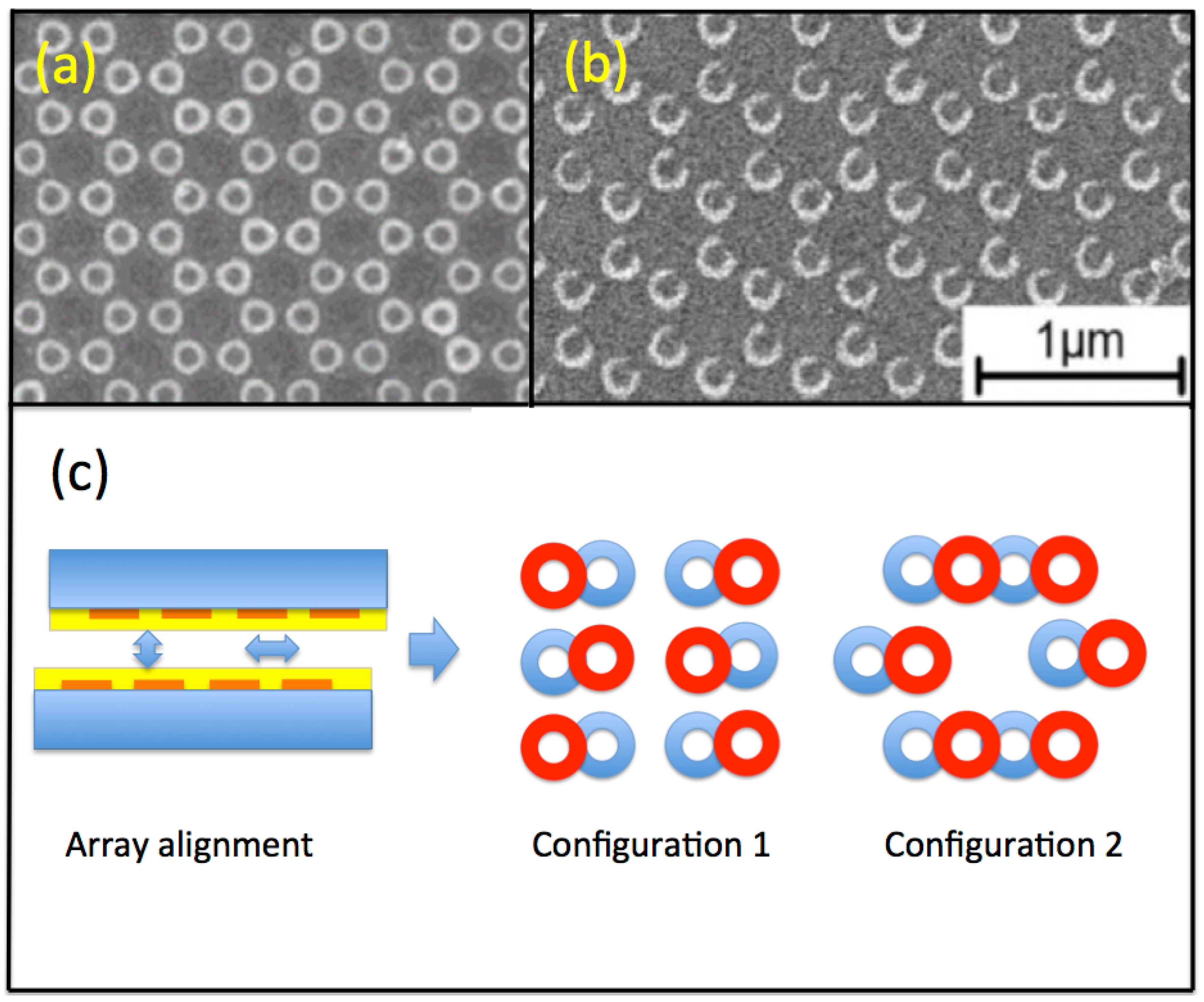
The effects discussed above can be studied via the electromagnetic response of arrays of metallic nanorings. These form photonic/plasmonic crystals with enhanced electromagnetic response [8]. Such structures can be made by a variety of techniques, including electron beam lithography (EBL), as well as shadow nanosphere lithography (SNL) [16,17]. This last technology provides an inexpensive route to complex periodic nanostructures, including nanorings. Figure 8a,b shows scanning electron microscopy (SEM) images of arrays of metallic nanorings (circular and c-shaped, respectively) deposited on a substrate using SNL. Such arrays can be used as a basis for corresponding arrays of coupled nanorings, which will have a very pronounced electromagnetic response depending on the physics of the inter-ring coupling and non-linear, intra-ring losses. To obtain the coupled nanoring arrays, we make two copies of an array (e.g., circular rings), as shown schematically in Figure 8c, left panel. Each copy is an array, deposited on a transparent, but lossy substrate (blue), and with the rings (orange) coated with a dielectric film (yellow). The two copies are sandwiched together, but depending on their relative offset, various configuration overlaps can be achieved. For example, one can perfectly align the rings (not shown) and therefore realize a uniform coupling (). However, by shifting the two arrays relative to each other, one can achieve localized coupling as discussed above (Configuration 1), or multiple localized coupling (Configuration 2). In Configuration 2, one has a more complicated situation, with some rings coupled only to single rings in the other array and some to multiple rings (in both arrays). In addition, even in Configuration 1, one can achieve a pair of localized coupling regions by making horizontal shift adjustments. The local coupling can also be realized by tilting rings with respect to each other, since the strength of the coupling is proportional to the distance. One can also use inhomogeneous filling of the inter-ring space.
Experimentally-realizable, more complex configurations could be of interest, and we will study the corresponding models elsewhere.
The physics described in previous sections relies on sufficiently large non-linear absorption losses. These can be controlled by choosing highly non-linear materials for the substrates (or substrate coatings), such as organic semiconductors, e.g., acetoacetanilide [18]. Another way to control the intra-ring nonlinear absorption would be to employ lossy metals for the body of the ring, or use the c-shaped rings, as shown in Figure 8b, with a nonlinear material coating in the opening. Such processing is possible [19]. The inter-ring coupling can be easily controlled via the dielectric coating (yellow colored layer in the left panel of Figure 8c). Furthermore, if the substrates could be made conducting, the bias across the pair could control the inter-ring coupling, as well, relying on the non-linearity of the current-voltage characteristics of these metal-insulator-metal (MIM) structures.
8. Conclusions
In this work, we continued our investigation of simple ring-shaped nonlinear waveguides in the presence of linear gain and nonlinear dissipation, adding local coupling between two channels. We have identified stationary and dynamic solutions both in the case of narrow and broad coupling. These solutions represent different types of symmetry breaking, corresponding to bifurcations of fixed points (stationary solutions) and of limiting cycles (symmetric and asymmetric oscillatory solutions). Dynamic solutions, connected with vortex generation, allow us both to control channel populations and generate vortex states in the system. We propose the experimental realization of our model in a nanoplasmonic system.
Supplementary Materials
Animations of system oscillations are available online at https://www.mdpi.com/2073-8994/10/6/195/s1. All frames consist of top frame, that shows absolute values of both wavefunctions (blue and red curves) and rescaled coupling potential (green curve), and bottom frame, which shows relative phases in both rings. Phases are plotted so that point for blue curve is fixed at 0, to eliminate phase oscillations term. All simulations are performed for .
Author Contributions
M.T. and V.V.K. have introduced the model, and performed the analytical investigation. A.R. and N.V.H. have performed numerical calculations, M.G. and K.K. analyzed the model and proposed experimental realization. All the authors took part in formulating the results and drafting the paper.
Acknowledgments
The work was supported by the Polish National Science Centre 2016/22/M/ST2/00261 (A.R. and M.T.). N.V.H. was supported by Vietnam National Foundation for Science and Technology Development (NAFOSTED) under grant number 103.01-2017.55. M.G. acknowledges the funding by the Guangdong Innovative and Entrepreneurial Team Program titled "Plasmonic Nanomaterials and Quantum Dots for Light Management in Optoelectronic Devices" (No. 2016ZT06C517).
Conflicts of Interest
The authors declare no conflict of interest.
References
- Peng, B.; Özdemir, Ş.K.; Lei, F.; Monifi, F.; Gianfreda, M.; Lu, G.; Long, L.G.; Fan, S.; Nori, F.; Bender, C.M.; et al. Parity–time-symmetric whispering-gallery microcavities. Nat. Phys. 2014, 10, 394–398. [Google Scholar] [CrossRef] [Green Version]
- Chang, L.; Jiang, X.; Hua, S.; Yang, C.; Wen, J.; Jiang, L.; Li, G.; Wang, G.; Xiao, M. Parity-time symmetry and variable optical isolation in active-passive-coupled microresonators. Nat. Photon. 2014, 8, 524–529. [Google Scholar] [CrossRef]
- Peng, B.; Özdemir, Ş.K.; Rotter, S.; Yilmaz, H.; Liertzer, M.; Monifi, F.; Bender, C.M.; Nori, F.; Yang, L. Loss-induced suppression and revival of lasing. Science 2014, 346, 328–332. [Google Scholar] [CrossRef] [PubMed] [Green Version]
- Liertzer, M.; Ge, L.; Cerjan, A.; Stone, A.D.; Tuüreci, H.E.; Rotter, S. Pump-Induced Exceptional Points in Lasers. Phys. Rev. Lett. 2012, 108, 173901. [Google Scholar] [CrossRef] [PubMed]
- Hodaei, H.; Miri, M.-A.; Heinrich, M.; Christodoulides, D.N.; Khajavikhan, M. Parity-time-symmetric microring lasers. Science 2014, 346, 975–978. [Google Scholar] [CrossRef] [PubMed]
- Li, Y.; Abolmaali, F.; Allen, K.W.; Limberopoulos, N.I.; Urbas, A.; Rakovich, Y.; Maslov, A.V.; Astratov, V.N. Whispering gallery mode hybridization in photonic molecules. Laser Photon. Rev. 2017, 11, 1600278. [Google Scholar] [CrossRef]
- Gao, T.; Li, G.; Estrecho, E.; Liew, T.C.H.; Comber-Todd, D.; Nalitov, A.; Steger, M.; West, K.; Pfeiffer, L.; Snoke, D.W.; et al. Chiral Modes at Exceptional Points in Exciton-Polariton Quantum Fluids. Phys. Rev. Lett. 2018, 120. [Google Scholar] [CrossRef] [PubMed]
- Wang, Y.; Plummer, E.W.; Kempa, K. Foundations of Plasmonics. Adv. Phys. 2011, 60, 799–898. [Google Scholar] [CrossRef]
- Huet, V.; Rasoloniaina, A.; Guillemé, P.; Rochard, P.; Féron, P.; Mortier, M.; Levenson, A.; Bencheikh, K.; Yacomotti, A.; Dumeige, Y. Millisecond Photon Lifetime in a Slow-Light Microcavity. Phys. Rev. Lett. 2016, 116, 133902. [Google Scholar] [CrossRef] [PubMed]
- Hung, N.V.; Zegadlo, K.B.; Ramaniuk, A.; Konotop, V.V.; Trippenbach, M. Modulational instability of coupled ring waveguides with linear gain and nonlinear loss. Sci. Rep. 2017, 7, 4089. [Google Scholar] [CrossRef] [PubMed]
- Sigler, A.; Malomed, B.A. Solitary pulses in linearly coupled cubic-quintic Ginzburg-Landau equations. Phys. D Nonlinear Phenom. 2005, 212, 305–316. [Google Scholar] [CrossRef]
- Chembo, Y.K.; Menyuk, C.R. Spatiotemporal Lugiato-Lefever fromalism for Kerr-comb generation in whispering-gallery-mode resonators. Phys. Rev. A 2013, 87, 053852. [Google Scholar] [CrossRef]
- Saito, H.; Ueda, M. Bloch Structures in a Rotating Bose-Einstein Condensate. Phys. Rev. Lett. 2004, 93, 220402. [Google Scholar] [CrossRef] [PubMed]
- Bludov, Y.V.; Konotop, V.V. Acceleration and localization of matter in a ring trap. Phys. Rev. A 2007, 75, 053614. [Google Scholar] [CrossRef]
- Agrawal, G.P. Nonlinear Fiber Optics, 3rd ed.; Academic Press: San Diego, CA, USA, 2001; ISBN 0-12-045143-3. [Google Scholar]
- Kosiorek, A.; Kandulski, W.; Chudzinski, P.; Kempa, K.; Giersig, M. Shadow nanosphere lithography: Simulation and experiment. Nano Lett. 2004, 47, 1359–1363. [Google Scholar] [CrossRef]
- Kosiorek, A.; Kandulski, W.; Glaczynska, H.; Giersig, M. Fabrication of nanoscale rings, dots, and rods by combining shadow nanosphere lithography and annealed polystyrene nanosphere masks. Small 2005, 14, 439–444. [Google Scholar] [CrossRef] [PubMed]
- Vijayan, N.; Ramesh Babu, R.; Gopalakrishnan, R.; Ramasamy, P. Some studies on the growth and characterization of organic nonlinear optical acetoacetanilide single crystals. J. Cryst. Growth 2004, 267, 646–653. [Google Scholar] [CrossRef]
- Gwinner, M.C.; Koroknay, E.; Fu, L.; Patoka, P.; Kandulski, W.; Giersig, M.; Giessen, H. Periodic Large-Area Metallic Split-Ring Resonator Metamaterial Fabrication Based on Shadow Nanosphere Lithography. Small 2009, 53, 400–406. [Google Scholar] [CrossRef] [PubMed]
Figure 1.
Absolute values of antisymmetric stationary states after propagation time in the coupled double-ring system (1) obtained for the initial conditions (4) with and . Left panel: Antisymmetric states calculated for different coupling strengths and fixed coupling width (). The black line represents the homogeneous state for the respective uncoupled system. Right panel: Antisymmetric states calculated for different coupling widths and fixed normalized coupling ().

Figure 2.
Absolute value (left) and the phase (right) of stationary solutions observed in the case of narrow coupling . The black curve represents antisymmetric solution (), and blue and red curves show the absolute value of both channels in the asymmetric state (). The phase oscillating term is eliminated, so that . The relative phase of the second channel in the antisymmetric case is not shown, as . Note that equals zero at .

Figure 3.
Top row: Contour plots of absolute values and phases of the propagated wavefunction in the stationary (asymptotic) regime for two different coupling strengths and the fixed width . The phase oscillation term is eliminated, so that . Center row: Norms in both channels ( and ) during propagation from initial perturbed symmetric homogeneous states, defined in Equation (4). Bottom row: Norms of both channels and average during one period of oscillations in the limit cycle regime. Note that we shifted the time in order to show directly the length of the period of oscillations. Panels on the left show symmetric oscillations for , and panels on the right show asymmetric oscillations for .
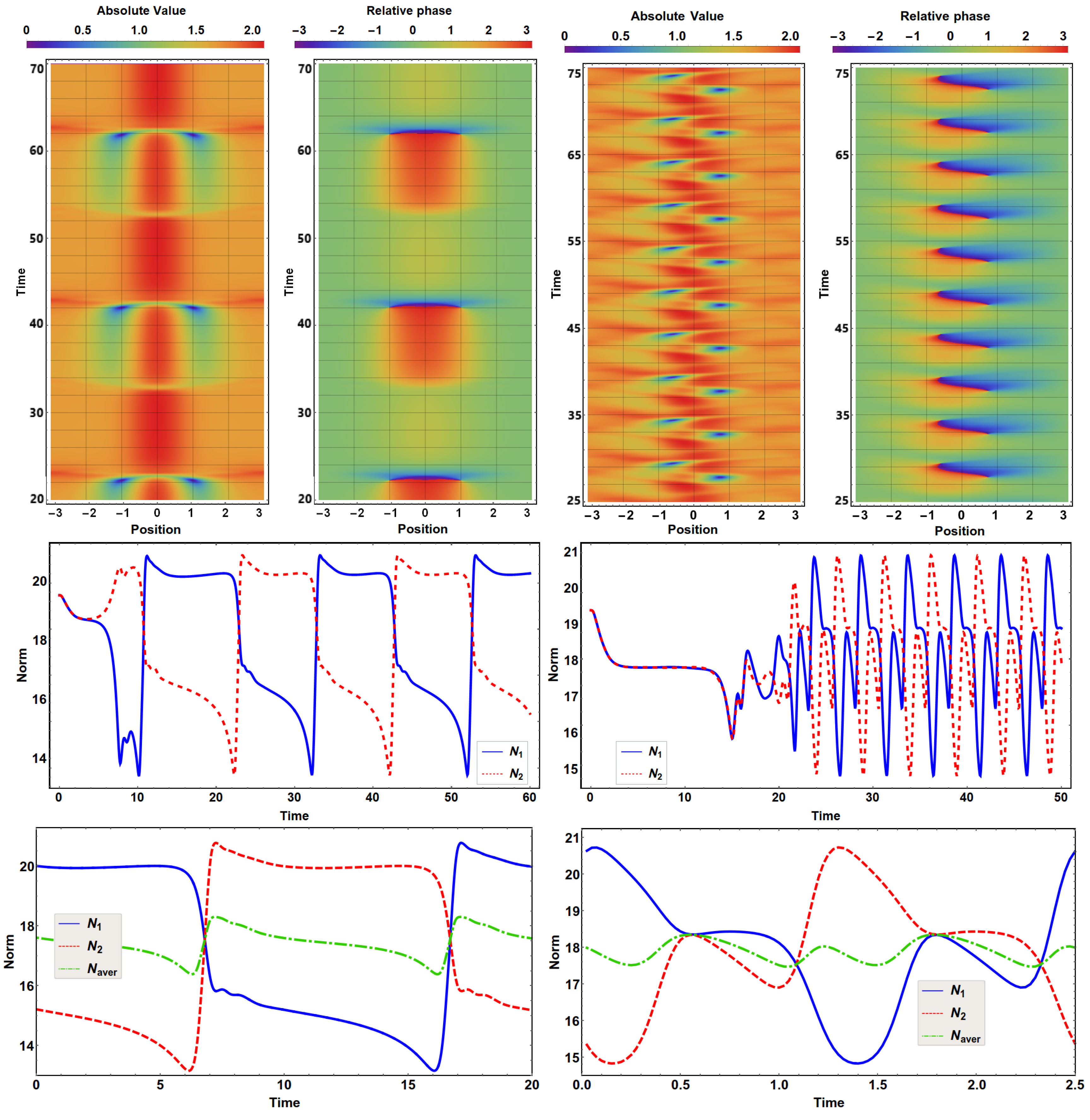
Figure 4.
Snapshots of wavefunction propagation, representing the half period of symmetric oscillations with coupling strength , , and . All frames are presented in pairs, where the top frames (a1-h1) show the absolute values of both wavefunctions (blue and red curves) and the rescaled coupling potential (green curve), while the bottom frames (a2-h2) show the relative phases in both rings. Phases are plotted so that point for the blue curve is fixed at zero, to eliminate the phase oscillation term.

Figure 5.
Snapshots of wavefunction propagation, representing the full period of asymmetric oscillations with coupling strength in the broad coupling regime, , and . All frames are presented in pairs; the top frames (a1–l1) show absolute values of both wavefunctions (blue and red curves) and rescaled coupling potential (green curve), and bottom frames (a2–l2) show relative phases in both rings. The phase oscillation term was eliminated as in Figure 4.

Figure 6.
Left panel: Frequency of the oscillations of the limit cycle solutions for three different values of . Symmetric oscillations (see Figure 4) are marked as continuous lines and asymmetric (see Figure 5) with dashed lines. The other parameters: , . Right panel: The norm in both channels at , where the blue line on the left panel has discontinuity. We observe that after initial propagation (not shown), the system develops into a symmetrically-oscillating state (shown in the time interval from to ) and after several (typically three or four, depending on the initial perturbation) periods of oscillation, the system finally evolves into asymmetrical oscillations.

Figure 7.
Snapshots of wavefunction propagation, representing relaxation from the point of vortex generation (Point b from Figure 5) after turning off the coupling, for and . All frames are presented in pairs; the top frames (a1–d1) show absolute values of both wavefunctions (blue and red curves), and bottom frames (a2–d2) show the relative phases in both rings. The phase oscillation term was eliminated as in Figure 4.

Figure 8.
(a,b) SEM images of the circular and c-shaped nanorings produced by shadow nanosphere lithography (SNL). (c) Schematic of the assembly of the coupled nanoring arrays (left panel) and the resulting examples of possible offset-dependent ring alignment configurations.
Figure 8.
(a,b) SEM images of the circular and c-shaped nanorings produced by shadow nanosphere lithography (SNL). (c) Schematic of the assembly of the coupled nanoring arrays (left panel) and the resulting examples of possible offset-dependent ring alignment configurations.
© 2018 by the authors. Licensee MDPI, Basel, Switzerland. This article is an open access article distributed under the terms and conditions of the Creative Commons Attribution (CC BY) license (http://creativecommons.org/licenses/by/4.0/).
Share and Cite
MDPI and ACS Style
Ramaniuk, A.; Hung, N.V.; Giersig, M.; Kempa, K.; Konotop, V.V.; Trippenbach, M. Vortex Creation without Stirring in Coupled Ring Resonators with Gain and Loss. Symmetry 2018, 10, 195. https://doi.org/10.3390/sym10060195
AMA Style
Ramaniuk A, Hung NV, Giersig M, Kempa K, Konotop VV, Trippenbach M. Vortex Creation without Stirring in Coupled Ring Resonators with Gain and Loss. Symmetry. 2018; 10(6):195. https://doi.org/10.3390/sym10060195
Chicago/Turabian StyleRamaniuk, Aleksandr, Nguyen Viet Hung, Michael Giersig, Krzysztof Kempa, Vladimir V. Konotop, and Marek Trippenbach. 2018. "Vortex Creation without Stirring in Coupled Ring Resonators with Gain and Loss" Symmetry 10, no. 6: 195. https://doi.org/10.3390/sym10060195
Note that from the first issue of 2016, this journal uses article numbers instead of page numbers. See further details here.