Fluid-Solid Boundary Handling Using Pairwise Interaction Model for Non-Newtonian Fluid

1
School of Computer and Communication Engineering, University of Science and Technology Beijing, Beijing 100083, China
2
Beijing Key Laboratory of Knowledge Engineering for Materials Science, Beijing 100083, China
3
Department of ICT & Natural Sciences, Norwegian University of Science and Technology, 6009 Aalesund, Norway
4
Beijing No. 4 High School, Beijing 100034, China
*
Authors to whom correspondence should be addressed.
Symmetry 2018, 10(4), 94; https://doi.org/10.3390/sym10040094
Submission received: 28 February 2018
/
Revised: 29 March 2018
/
Accepted: 31 March 2018
/
Published: 3 April 2018
(This article belongs to the Special Issue Symmetry in Cooperative Applications III)
Abstract
:In order to simulate fluid-solid boundary interaction for non-Newtonian Smoothed Particle Hydrodynamics (SPH) fluids, we present a steady and realistic fluid-solid boundary handling method using symmetrical interaction forces. Firstly, we use the improved SPH method to model the non-Newtonian fluid. Secondly, the density of boundary particle is created into the calculation of fluid-solid interaction forces. Besides, we apply friction conditions to constrain the fluid particles at the boundary. Finally, we apply the predictive-corrective scheme to correct the density deviation and improve boundary computing efficiency. The experiment confirms the feasibility for the interaction between non-Newtonian fluid and solid objects with this method. At the same time, it reflects the viscous characteristics and ensures the physical properties of non-Newtonian fluid. In addition, compared to existing methods, this method is more stable and easier to implement.
1. Introduction
Fluid phenomenon is common in nature, daily life and industry. Fluid simulation and fluid animation have always been the significant content in computer graphics, visualization, virtual reality, etc. According to Newton theory, the viscosity of fluid is constant, such as water, alcohol, and light oil. However, the study of posterity shows that the viscosity of fluid is actually not constant, the previous studies in fluid simulation mainly focused on Newtonian fluid and they seldom involved non-Newtonian fluids with nonlinear physical properties. The simulation for non-Newtonian fluid is more challenging based on the complexity of its constitutive equation and flow characteristics [1].
During the last few years, Smooth Particle Hydrodynamics (SPH) [2] has become a popular approach for simulating Newtonian fluid since it is simple and efficient in computation. However, there are several unsolved issues to simulate non-Newtonian fluid with SPH. Among those issues, fluid-solid boundary handling of non-Newtonian fluid is a compelling topic. For instance, some simulations are tried for the phenomena as stirring honey with a spoon or adding sugar to coffee. While interaction between non-Newtonian fluid and solid objects seems to be straightforward as Newtonian fluid with solid. However, Non-Newtonian fluid differentiates from Newtonian fluid in bending, rotating, Weissenberg effect and a variable viscosity [3]. Therefore, specific boundary conditions should be considered when dealing with fluid-solid interaction of non-Newtonian fluid.
In order to solve the problem of interaction between non-Newtonian fluid and solid using the SPH method, we propose a steady and vivid fluid-solid boundary handling method. Firstly, we build a novel SPH model for non-Newtonian fluid. Secondly, a symmetrical interaction model is created to compute the forces between the fluid particle and the boundary particle, considering the density of the boundary particle. Finally, the friction boundary condition is enforced to constrain the fluid particles at the boundary while using a predictive-corrective scheme [4] to improve computing accuracy and efficiency.
The paper continues with a discussion of related work in Section 2. We introduce non-Newtonian fluid simulation in Section 3. Fluid-solid boundary handing of non-Newtonian fluid are explained in Section 4. We demonstrate examples of our approach in Section 5, and finally, conclusions and future work are discussed in Section 6.
2. Related Works
Non-Newtonian fluid plays an important role in engineering and nature, with very different types and different rheological properties. Non-Newtonian fluid simulation can be divided into two categories: grid methods and grid free methods. With the grid free methods, most of the SPH fluid simulations are based on Newtonian fluid. Due to the viscosity of non-Newtonian fluid being nonlinear, the motion of fluid is more complicated. Müller et al. proposed the Laplace form of viscosity [2]. They built a point-based animation modeling method to simulate the fluid with high elasticity and high plasticity [5]. Goktekin et al. [3] used explicit Euler method to simulate the process of melting wax block based on von Mises’s yield condition. They proposed a quasi-linear plasticity model to control viscosity change when the solid gradually becomes non-Newtonian fluid. Monaghan et al. [6] proposed the Laplace approximation of artificial viscosity and velocity field, which is widely used. Their work later was improved by Schechter [7] and Macklin [8]. Losasso et al. [9] conducted unified modeling of fluid with different densities and different viscoplastic by extending the method of particle level set. Batty et al. [10] found that the strain rate term and the Laplace term of non-Newtonian fluid needs to be calculated under divergence-free velocity field. Hence, they corrected the viscosity by pressure and proposed an implicit and stable method based on Marked-and-Cell (MAC) method. However, this method could not simulate Newtonian fluids with high viscosity. Besides, for non-Newtonian fluids, the viscous force can also be derived from the strain tensor. Although the Laplace approximation is physically correct for incompressible fluids, there are still other approximation methods to smooth the velocity field. For example, Steele [11] uses relative speed to calculate the viscous force. Their method significantly improves the stability of SPH simulation of low viscous fluid, but it is not efficient for high viscous fluid.
In a high-viscous fluid, the explicit methods are limited by the time step. They are only suitable to small time step. The large time step will generate instability so that the particles will explode. Paiva et al. used a generalized Newtonian fluid method for modeling [12], implemented the process of the high viscosity non-Newtonian fluid melting to low viscosity fluid. In this method, the fluid properties depend on the temperature of simulation scenario. The fluid viscosity is controlled by the jump number [13]. Takahashiet et al. [14] proposed a viscous implicit algorithm, which was improved by the Euler algorithm from Batty [10]. Peer et al. [15] further used implicit equation to simulate the high viscous fluid and reconstruct the velocity field from the target velocity gradient. This gradient contains the desired shear rate damping and retains the velocity divergence to offset the density deviation. This method can use a larger time step and does not generate the particle explosion. Rafiee et al. [16] proposed a SPH method for free surface, which can be used to simulate Newtonian fluid and viscoplastic fluid. It can simulate the bending of viscous fluid. Fan et al. [17] used the real polymer state equation to describe the relationship between pressure and non-Newtonian fluid viscosity to simulate the flow of polymer with high viscosity and high pressure. Andrade et al. [18] presented a unified simulation method for viscous Newtonian fluid and sheared thinning non-Newtonian fluid using Cross model. However, this method can only simulate low viscosity fluid. In addition, when the time step is getting larger, it appears unstable.
In order to improve the fidelity of fluid simulation, fluid-solid boundary handling is also an important field of study. There are many trial works on solid boundary particle sampling. Keiser et al. [19] calculated the pressure effect on the boundary, sampled the solid as particles, so the fluid-solid interactions are based on particles. However, they ignored the viscous force. Becker et al. [20] modeled the fluid-solid boundary handling with direct force method. The main idea in this method is to avoid the fluid particles penetrating according to the corrective location. In addition, the asymmetric friction model was used to simulate the effect of different sliding. However, this method does not satisfy the law of conservation of momentum and cannot simulate the interaction between fluid and multiple solid bodies. Solenthaler et al. [21] proposed a unified particle simulation framework to simulate the interactions between fluid and solids. This method is used to calculate the influence of solid particles while calculating the fluid density and various forces. Nevertheless, this method prevents fluid particles penetrating solid surface by pressure. The problem is that if we make large pressure for high relative speed, the fluid particles will penetrate solid particles. In order to avoid this, the simulation must use a smaller time step. Fluid-solid boundary handling for non-Newtonian fluid brings us new challenges as the non-Newtonian fluid viscosity is constantly changing, and generates specific effects such as bending, rotation and Weissenberg effect. Therefore, when dealing with the fluid-solid boundary of the non-Newtonian fluid, the friction boundary conditions should be considered to ensure the physical properties of non-Newtonian fluid [22].
3. Non-Newtonian Fluid Simulation
In recent years, the SPH method is widely used in the field of fluid simulation. Traditional SPH fluid model aims at ideal Newtonian fluid [23]. For non-Newtonian fluid, the relationship between the viscosity and shear rate are highly nonlinear. This results in the Newtonian fluid control model being unable to be directly applied to non-Newtonian fluid.
In this section, firstly, we briefly introduce the difference between Newtonian and non-Newtonian fluid. Secondly, we explain Cross Model [18,24] and improve the SPH method for non-Newtonian fluid [4]. Finally, we consider fluid-solid boundary conditions to help the SPH approximation with non-Newtonian fluid.
3.1. Comparison of Newtonian and Non-Newtonian Fluid
In Rheology, liquids include two classes, that is Newtonian and Non-Newtonian fluid. Newtonian fluids obeys Newton’s hypothesis which has perfect viscosity. The viscosity of Newtonian fluid remains constant at all possible shear rate conditions for a given temperature. Because of Newtonian fluid’s purity and the lack of dispersion, they are much easier to measure than non-Newtonian fluids.
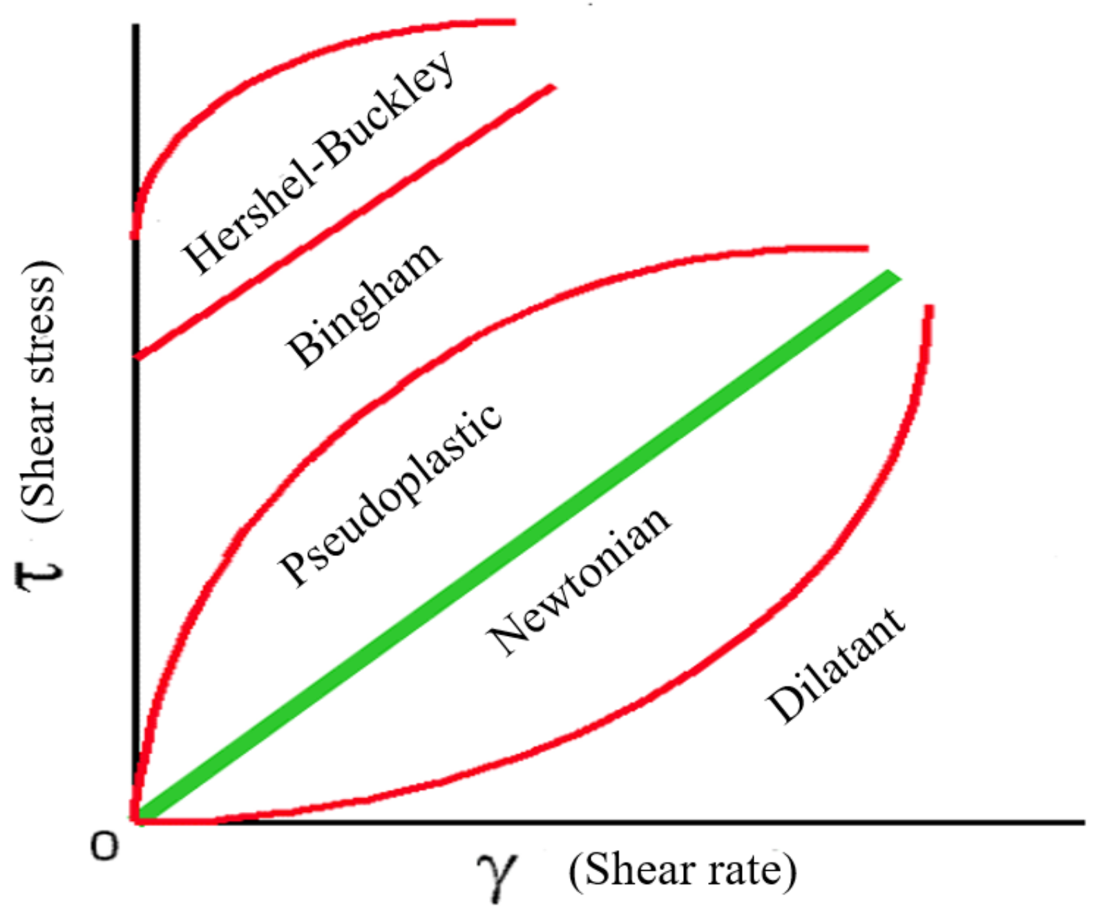
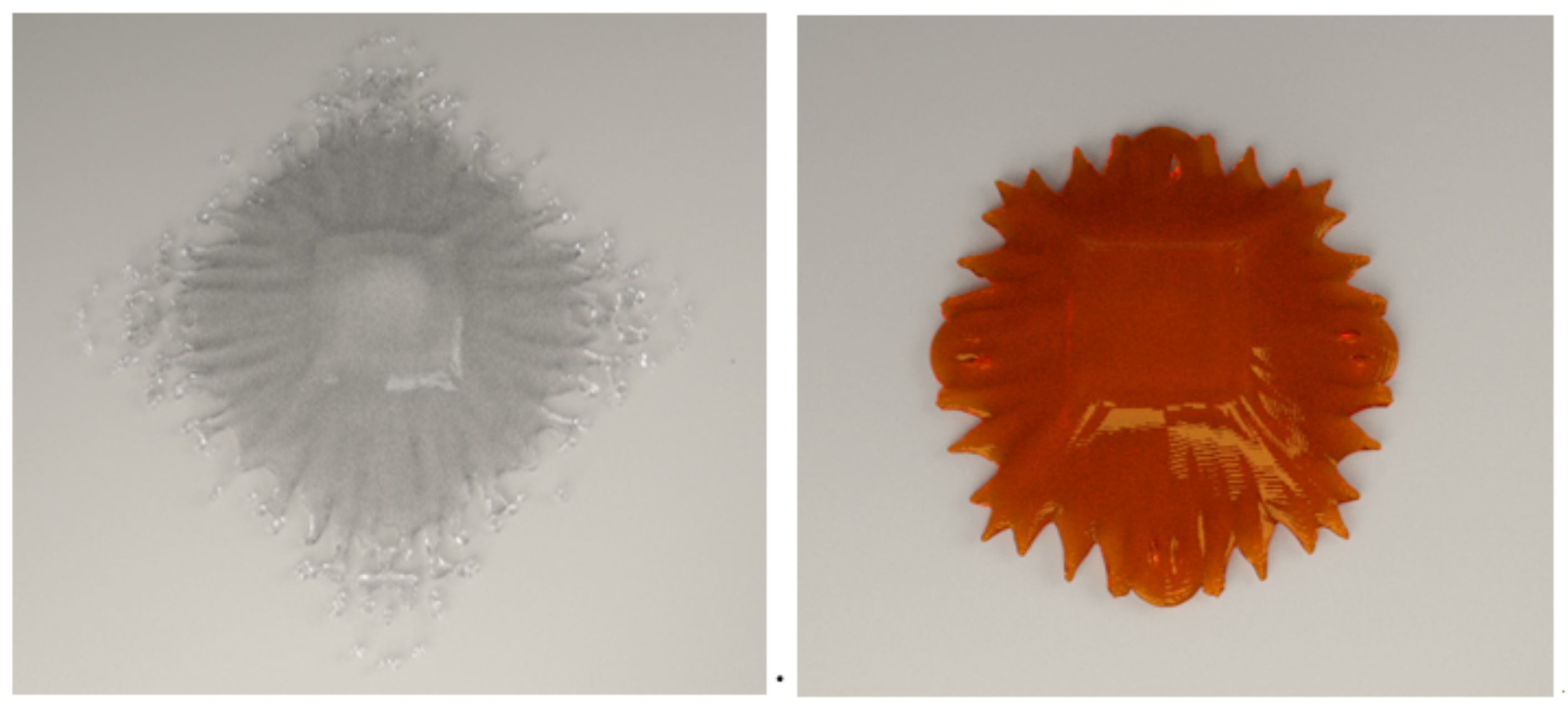
Non-Newtonian fluid does not have a constant ratio between shear rate and shear stress, which means it is unpredictable in how its shear stress changes according to the shear rate with the fluid’s own characteristics. In this paper, we focus on the pseudoplastics fluid, in which the viscosity decreases as the shear increases. In contrast to Newtonian fluids model, shear-thinning fluid’s behavior is not stable. Once the viscosity changes, the fluid structure changes, that is, the changing viscous force causes the molecules or particles to be reordered. Therefore, the essential difference between Newtonian and non-Newtonian fluids is the viscosity (as shown in Figure 1). In this paper, shear-thinning non-Newtonian fluid is modeled by the control equation with Cross Model (see Section 3.2). Figure 2 shows the simulation effect of Newtonian fluid and non-Newtonian fluid. From the picture, the edge of Newtonian fluid appears splash while non-Newtonian fluid does not have this phenomena for its high viscosity. Note that we do not consider the effect of temperature and elastoplastic.
3.2. Control Equation with Cross Model
Because non-Newtonian fluid is a continuous medium, the fluid motion should satisfy the conservation of mass and energy. The mass of the fluid particles in the SPH scheme remains constant, so the total mass of non-Newtonian fluid systems remains conserved. For non-Newtonian fluids possessing elastoplastic, the viscous stress tensor is added to the control equation, in order to maintain the energy conservation of non-Newtonian fluid motion. Thus, the control equation of non-Newtonian fluid can be expressed as:
t denotes the time. is the velocity of the fluid. is the density. p is the pressure. is the viscous stress tensor. is the external force density field.
In Equation (1), the left expression is the acceleration of the fluid particle, and the right expression is the component of the acceleration, the term is the pressure acceleration and expresses the viscous acceleration of non-Newtonian fluid. Viscous acceleration is an important physical item that is distinguished from Newtonian fluid.
In order to better simulate the physical properties of non-Newtonian fluids, such as bending, rotating and folding, we use the Cross Model to deal with non-Newtonian fluids. In contrast to the Newtonian fluid model, this Cross Model takes the viscous stress tensor into account. Assuming non-Newtonian fluid rate of deformation tensor is , the and M satisfy nonlinear function relationship between:
In Equation (2), is the dynamic viscosity and M is the shear rate. In Equation (3), is the trace of the matrix.
The Cross Model can better perform the shear thinning properties of non-Newtonian fluids, the following relationship between and M is:
In Equation (4), I and n are the control parameters of fluid viscosity. is the upper limit of viscosity under the low shear rate, and is the lower limit of viscosity under high shear rate. Their unit is .
From there, we can deduce that when and the dynamic viscosity of the fluid is a fixed value , which means the fluid is Newtonian fluid now. It can be found that this method implements a unified model for non-Newtonian fluid and Newtonian fluid.
3.3. Non-Newtonian Fluid Simulation with SPH
The SPH scheme is essentially a method of interpolation of weight functions [25]. This method interpolates approximate calculation of the physical properties of fluid particles, such as mass, velocity and pressure. The continuous integral formula can be approximated into a summation formula by dividing the continuous fluid into N small particles. The assumption behind this is that each particle has independent mass and occupies the independent space.
In Equation (5), and represent the mass and density of particle j. denotes the position of particle j. The function is the smoothing kernel with core radius h. Equation (5) shows that the interpolation of discrete particles can be calculated by smoothing kernel function when solving the value of particle i.
In SPH, the calculation formula of space derivative is:
Using the SPH method above, the density , pressure and viscosity of non-Newtonian fluid can be interpolated approximately. By substituting density into Equation (5), the density solution formula of non-Newtonian fluid can be obtained [25]:
We can see the computational cost of non-Newtonian fluid modeling is more expensive than Newtonian fluid. So, in order to reduce the calculation amount, the solution of pressure is as follows:
k is the intensity coefficient. is the relative density ( = 1000 kg/m).
The pressure may influence the non-Newtonian fluid to acquire the acceleration and motion. To calculate the acceleration of the non-Newtonian fluid pressure, is substituted into Equation (6), which can be obtained after symmetry [25]:
The viscous acceleration in Equation (1) can first calculate the deformation rate tensor of the fluid particle, in which:
By Equations (2) and (10), the viscous stress tensor of the fluid particles can be calculated, and the formula of the viscous acceleration can be obtained:
3.4. Fluid-Solid Boundary Conditions
In our method, we use fixed solid particles to represent the solid boundary. These boundary particles are similar to the fluid particles, which can help the SPH approximation with non-Newtonian fluid.
The pressure of boundary particle can prevent fluid particles from penetrating the solid objects. In order to ensure the boundary condition, the velocity of boundary particle is set to zero during the whole simulation process. These boundary particles are placed outside of the computational domain. The distances between the particles are equal to the initial distance of the fluid particles. The boundary here is composed of several layers of boundary particles. The width of the boundary particle layer is at least equal to the support radius of smooth kernel function, which is used to alleviate the problem of lacking particles at the boundary.
The other boundary condition is the non-stress condition of the momentum equation, which indicates that the total normal stress must be zero at the free surface [16]. In mathematics, it can be expressed as:
is the identity matrix. is the normal vector of the free surface.
4. Fluid-Solid Boundary Handling of Non-Newtonian Fluids
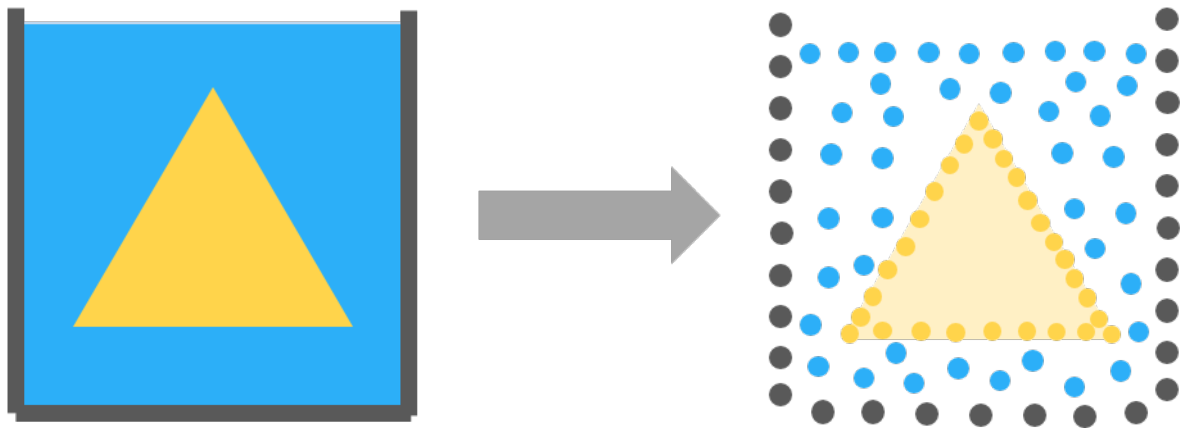
The basic treatment of fluid-solid boundary handling for non-Newtonian is similar to Newton fluid. However, non-Newtonian fluid has the characteristics of bending, rotating and climbing pole for its nonlinear viscosity, additional friction boundary conditions should be added for fluid-solid boundary. The fluid-solid interaction framework we adopt is shown in Figure 3. There are two types of solid that are container and triangle, and the blue part is non-Newtonian fluid. Before the simulation, the boundary of the container and the triangle object should be sampled to obtain the boundary particles. Then we create a series of interaction forces between fluid particles and boundary particles to realize the interaction between fluid and solid.
In this chapter, we first introduce the fluid-solid interaction force by sampling the boundary particles. Then we add the solid boundary contributions to the SPH scheme. We also use artificial viscosity to build a friction formula for fluid-solid boundary. In addition, we consider the frictional boundary conditions to constrain non-Newtonian fluid particles, in order to depict viscous properties of non-Newtonian fluids at the boundary. Finally, we select a novel predictive-corrective method [4] to improve the accuracy and efficiency of non-Newtonian fluid-solid boundary calculation.
4.1. Pairwise Interaction Model
4.1.1. Density Estimation of Solid Particle
Here we select the fast Poisson-disk sampling method [7,22] to sample the solid boundary. In this way, after getting the boundary particles distributed on the solid surface, we take the contribution of solid boundary particles in the SPH method:
is non-Newtonian fluid particle i. is the solid boundary particle k. As shown in Figure 4, the first sum item in Equation (13) is the sum of all the neighbor fluid particles of non-Newtonian fluid particles. The second sum item is the sum of all the adjacent solid boundary particles. This method can improve the boundary defect of the SPH method.
Note that if the mass of boundary particles is illogical or boundary sampling is non-uniform, it will bring unreasonable mass contribution for fluid particles that will lead to unstable density for fluid particles. Therefore, we choose a unified mass value of boundary particles as . As a result the volume of boundary particle does not depend on its mass, which can guarantee the stability of the fluid particle’s density. The volume of the boundary particle can be expressed as:
Therefore, Equation (13) will be improved by replacing the mass of the solid boundary particle with the volume term. For this purpose, the density contribution of solid boundary particles to fluid particles can be defined as follows:
The is the density of the fluid. Equation (13) can be changed to:
Consequently, choosing the appropriate solid surface reconstruction can solve the unstable phenomenon of fluid particle explosion or the fluid particles penetrating the solid. The solid boundary particle contribution is taken into account for the SPH method, in order to improve the stability of non-Newtonian fluid particles and solve the SPH boundary defect problem.
4.1.2. Fluid-solid Interaction Forces
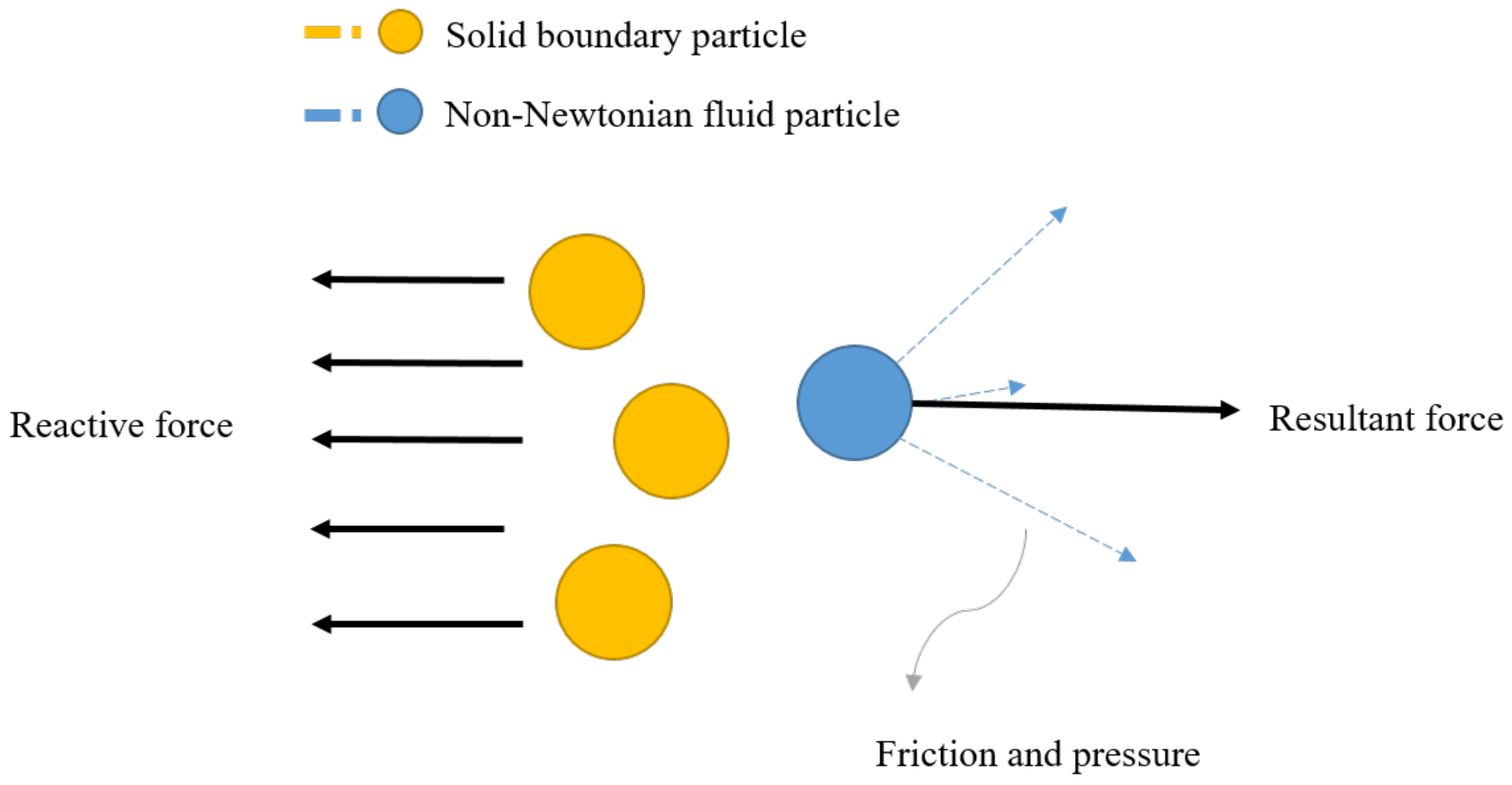
For interactions between solid boundary particles and fluid particles, pressure force, friction and reaction force are the three main forces (as shown in Figure 5). In order to simulate the interaction between a fluid particle and a solid boundary particle, we need to carefully deal with these three forces.
Pressure is a very important force in the interaction between fluids and solids. Here we consider the density contribution of solid boundary particles. Equation (15) is used to calculate the acceleration of the pressure:
We can see from the above equation that when the pressure of the fluid particle is negative, the solid boundary particle and the fluid particle are attracted to each other. The physical manifestation is the adsorption of the fluid on the solid surface. If we want to weaken or avoid adsorption, the pressure of the fluid particles should be treated separately for the positive and negative conditions.
Friction is another important force in the process of fluid-solid interaction. However, few previous works studied the friction characteristics of non-Newtonian fluid flow and fluid-solid boundary handling. We propose a more suitable friction algorithm for shear thinning non-Newtonian fluid in fluid-solid boundary handling. The basic idea is to learn from the artificial viscosity. The friction acceleration is expressed as follows:
. . is a tunable parameter. is the sound velocity in a fluid medium. . is to avoid .
When the fluid particles interact with solid particles, although the above method has solved the solid boundary pressure and friction force with fluid particles. The force of fluid particles and solid particles is not convenient to calculate near the fluid-solid boundary. Equations (17) and (18) gave the fluid particles force to solid boundary particles. According to Newton’s third law, the absolute value of action and reaction are equal. So the fluid particles of solid boundary particles force computation formula is as follows:
For the solid object, the resultant force and resultant torque are:
Equation (20) means the sum of all the boundary particle k of the solid. In Equation (21), is the position of particle k. means the center of mass of solid, × is the cross product of the vector. Finally, the resultant force and the moment of resultant force are transferred to the physics engine.
In conclusion, in the interaction between non-Newtonian fluid particles and solid boundary particles, we use the solid boundary particle density to calculate the pressure force of solid particles on fluid particles. A new formula for calculating the friction between non-Newtonian fluid particles and solid boundary particles is presented by reference to artificial viscosity. Newton’s third law is used to solve the computational problem of non-Newtonian fluid particles on solid boundary particles.
4.2. Friction Boundary Condition
Considering the non-Newtonian fluid, such as features of bending, rotation and the Weissenberg effect, we add friction boundary conditions to constrain non-Newtonian fluid particles at the boundaries [26]. This is to realize the viscous characteristics of non-Newtonian fluid at the boundary.
For this reason, the velocity of non-Newtonian fluid particles is decomposed into normal component and tangential component along the boundary. When boundary conditions are performed on the grid, friction is calculated according to Equation (18). While the normal component of the velocity is projected, the tangential component of the velocity is reduced accordingly. In the case of static friction, it is clamped to zero:
is the coulomb friction coefficient between non-Newtonian fluid and solid.
This is the important supplement for fluid-solid boundary handling of non-Newtonian fluid. Because in the discussion of Newtonian fluid’s boundary conditions, one slide condition is which means fluid sticks even the vertical surface, or another condition that may lead to reduce viscosity of tangential velocity, will never be stable.
4.3. Optimization with Predictive-Corrective Method
We apply the non-Newtonian fluid predictive-corrective method [4] to correct the density deviation and improve computing efficiency. This can solve the fluid local distortion and fault phenomenon created by the SPH numerical problem. The algorithm firstly calculates the pressure force generated by the pressure acceleration on the fluid particle according to the SPH summation equation [25]. Secondly, it sets a single strength coefficient for each particle:
Secondly, the fluid particles i also produce a pressure force on the neighbor particles j , which is a pair of interacting forces , namely . According to the prediction concept, a middle velocity value is set for non-Newtonian fluid particles. After the pressure correction, a velocity correction is obtained, as well as the neighbor particles . The velocity of fluid particle i is:
corresponds fluid particle density is [25]:
In Equation (28), is the density of the fluid particles. By default, the incompressible condition has been fulfilled in the last time step, . The velocity and position of the fluid particle i at the moment are updated as follows:
The intermediate velocity values of non-Newtonian fluid particles and their neighbor particles can obtain the expression of the intermediate density. However, this can be corrected by the particle velocity and their neighbor particles. The correction of the density deviation can be expressed as:
After the correction of pressure, we have to consider the fluid density density conditions. Equations (26) and (27) can be substituted into Equation (32):
We can also get the strength coefficient of the fluid particles by the transformation of the above equation:
In this method, for non-Newtonian fluid average density, we have to set a standard density deviation threshold (experiment ). If the deviation between the average density and standard density is greater than , we can use Equation (28) to calculate the center of the fluid particle density. Otherwise we will use Equation (33) to calculate each fluid particle i intensity coefficient .
5. Implementation and Results
This section is to verify the effectiveness of our method through experiments. Operation platform is the Intel Xeon E5-2687W v4 (8 cores, 3.0 GHz, 20 MB Cache) with 72 GB memory. Surface construction algorithm and simulation algorithm are implemented with C++ language using multi-threading technology. This algorithm uses space background grid hash lookup to search neighbor particles. We use the anisotropy method for surface reconstruction, employ OpenGL 3D graphics library to achieve real-time display simulation, and use Blender to implement offline rendering.
The first experiment is pouring water into a container. If the parameter in Equation (4), the fluid is Newtonian fluid with constant viscosity, as shown in Figure 6 (upper row). When the Newtonian fluid comes into contact with the container, the fluid particles are splashed by the action of boundary. Another situation is which means the fluid is non-Newtonian fluid. In the same scene, because the viscosity of non-Newtonian fluid is larger than Newtonian fluid, splash phenomenon is nonexistent and bending effect appears when the fluid particles collide with the boundary that can be viewed from the lower row in Figure 6. The settings and parameters are shown in Table 1.
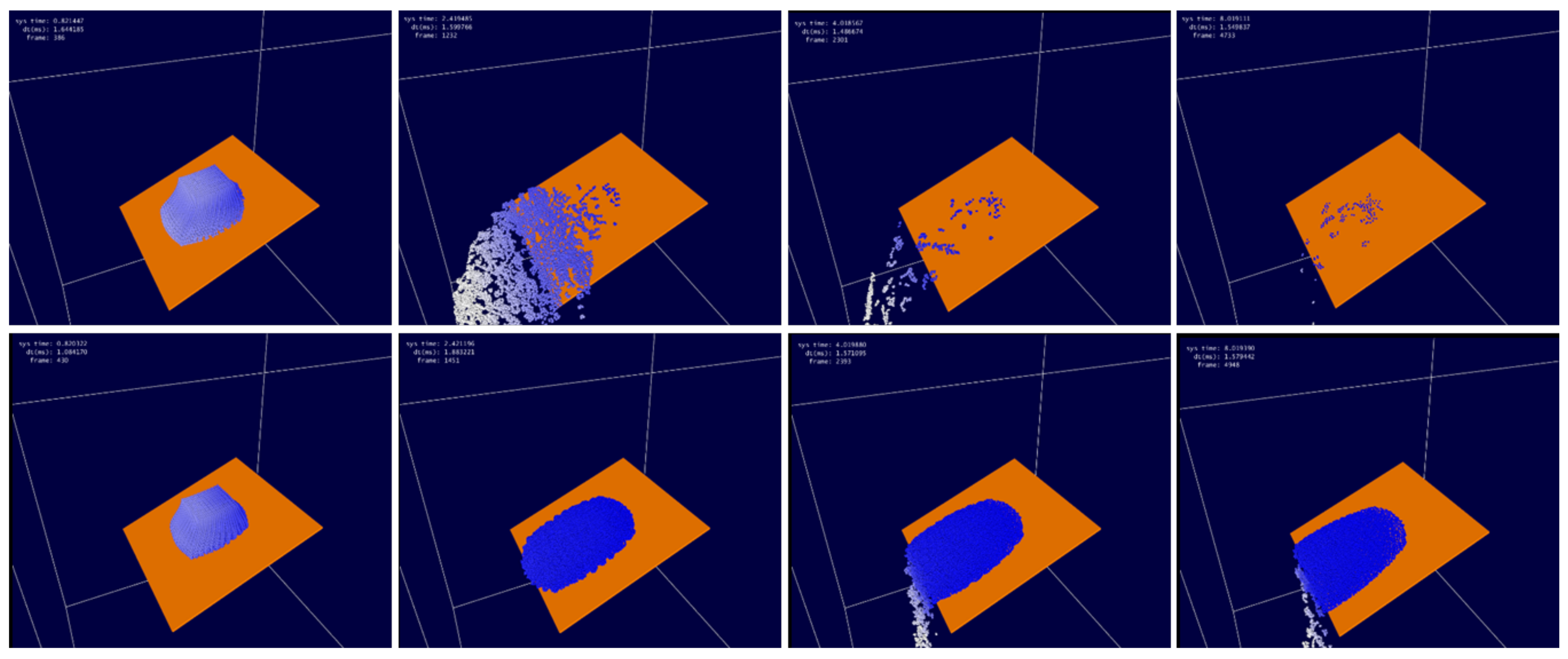
The second experiment is the friction boundary comparison of non-Newtonian fluid, as exhibited in Figure 7. The upper row shows the fluid volume flows along a slant board without friction boundary constraints. The fluid volume flows quickly after contact with the board. In about 8 s, the fluid particles all crept down. From the lower row, The boundary has a good constraint on the fluid particles with the friction conditions, so the flow process was slow and the fluids kept better viscous characteristics. Table 1 enumerates the experimental parameters and settings.
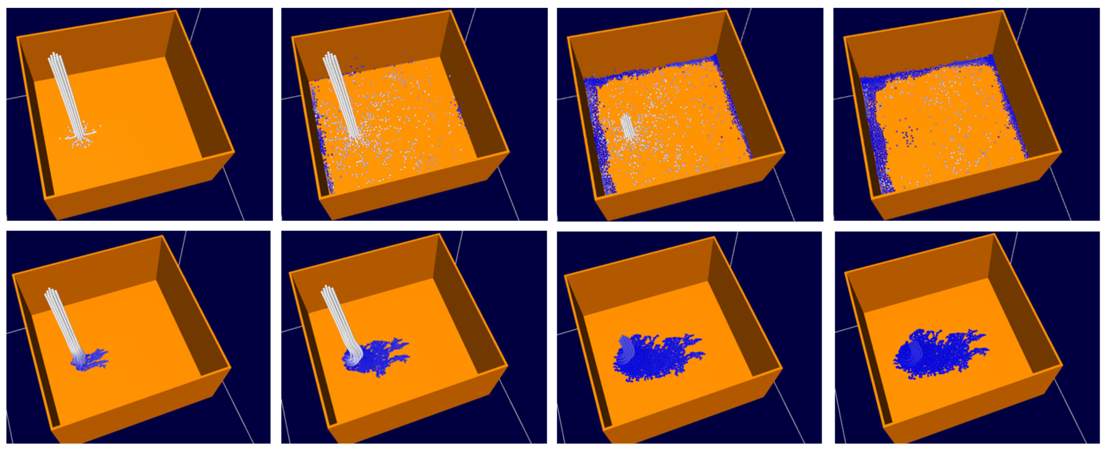
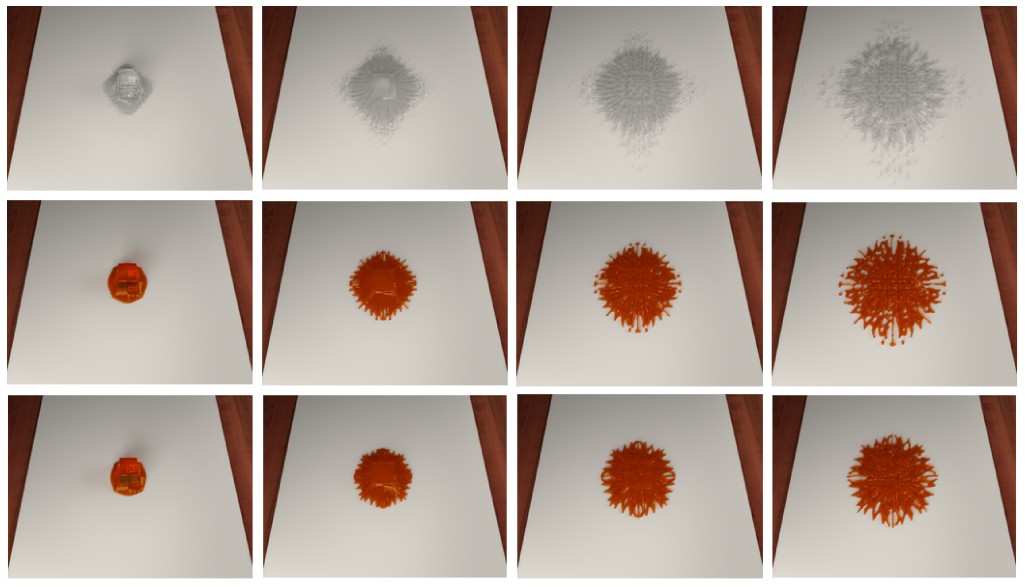
The third experiment is a fluid volume dropping on a planar solid object. This experiment compared Newtonian fluid [23] with non-Newtonian fluid for the boundary handling effect, as shown in Figure 8. As can be seen from the upper row of the figure, when the Newtonian fluid is interacting with the container boundary, the fluid particles are obviously dispersed due to lack of viscosity. However, the non-Newtonian fluid exhibits a strong adhesion effect (see the middle and lower row), and the particles are tightly bound together. Besides, comparing the middle row with the lower row, the viscous effect and absorbing solid effect is better when using our friction boundary condition. It is visible that fluid particles at the edge appear unreasonably fracture phenomenon in the middle row of Figure 8 while the lower row does not exhibit this problem. The settings and parameters are shown in Table 1.
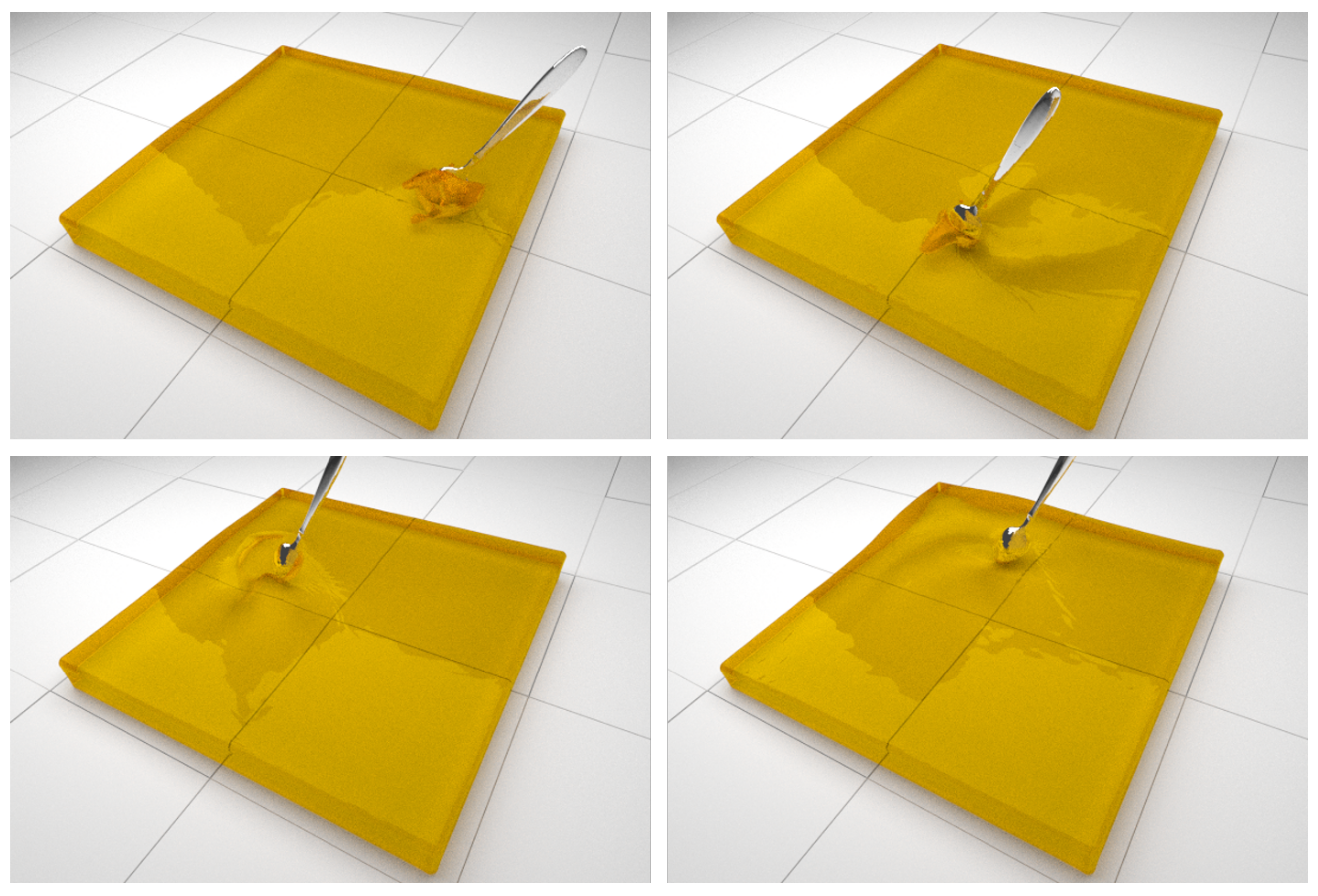
Figure 9 shows the stirring experiment of non-Newtonian fluid. The forth experiment is the honey fluid stirred with a spoon. During the stirring process, particles of Non-Newtonian fluid are closely gathered by the viscous force. There is no particle spatter problem even in large deformation positions. The interaction between the fluid and the spoon is almost the same as the actual effect. The settings and parameters are illustrated in Table 2.
The fifth experiment exhibits the simulation of melting butter in a plate (Figure 10). In this scene, the butter is gradually melting, particles are closely gathered by the viscous force which also well presents the characteristics of Non-Newtonian fluid. The visual effect is in accord with the real scenario. The settings and parameters are illustrated in Table 2.
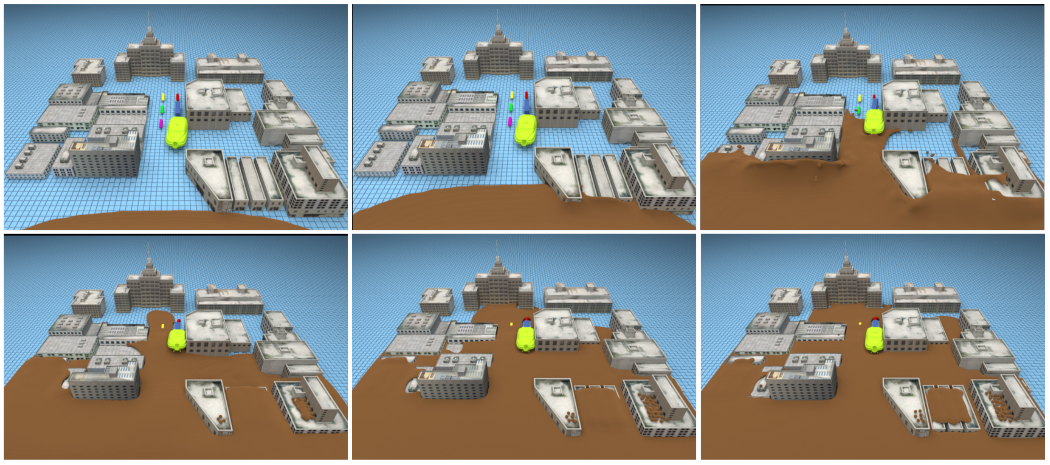
Figure 11 shows the simulated debris flow inundation buildings, vehicles and other scenes. In this experiment, the building was set to be immobile solid, and the vehicle was set to move solid. Different from flood disaster, the simulated debris flow in this experiment is highly viscous. In addition, the most violent part of the fluid particle and solid collision almost does not have the particle spatter problem. The fluid region with fast flow velocity has a strong wallop, so the fluid edge produced greater deformation. While the regions with slow flow velocity are more sticky which conforms to the physical characteristics of shear thinning non-Newtonian fluid. See Table 2 for parameters and settings.
6. Conclusions
In this paper, we propose a fluid-solid boundary handling method for SPH-based non-Newtonian fluid. A symmetrical interaction model is employed to compute the forces between fluid particle and boundary particle. We also considered the density of the boundary particle for interaction force calculation. In addition, the friction boundary condition is enforced to constrain the fluid particles at the boundary. The experimental results show that our method achieved the interaction of non-Newtonian fluid with solid and eliminated the splash phenomenon of non-Newtonian fluid particle, which preferably embodies characteristics of non-Newtonian fluid. However, for non-Newtonian fluid simulation and fluid-solid boundary handling, the computation cost is always a challenge. In future work, we will try to improve the efficiency of this method and we will extend it to large-scale scenarios.
Acknowledgments
The authors acknowledge the financial support from the National Key Research and Development Program of China (No. 2016YFB0700500), and the National Science Foundation of China (No. 61702036, No. 61572075).
Author Contributions
Xiaokun Wang conceived the framework and revised the paper; Runzi He wrote the paper; Xing Liu performed the experiments; Di Wu and Yuting Xu improved the English and polished the paper; all the work was done under the guidance of Xiaojuan Ban.
Conflicts of Interest
The authors declare no conflict of interest.
References
- Ellero, M.; Tanner, R.I. SPH simulations of transient viscoelastic flows at low Reynolds number. J. Non-Newton. Fluid Mech. 2005, 132, 61–72. [Google Scholar] [CrossRef]
- Müller, M.; Charypar, D.; Gross, M. Particle-based fluid simulation for interactive applications. In Proceedings of the ACM SIGGRAPH/Eurographics Symposium on Computer Animation, San Diego, CA, USA, 26–27 July 2003; Eurographics Association Press: Aire-la-Ville, Switzerland, 2003; pp. 154–159. [Google Scholar]
- Goktekin, T.G.; Bargteil, A.W.; O’Brien, J.F. A method for animating viscoelastic fluids. ACM Trans. Graph. (TOG) 2004, 23, 463–468. [Google Scholar] [CrossRef]
- Zhang, Y.; Ban, X.; Wang, X.; Liu, X. A Symmetry Particle Method towards Implicit Non-Newtonian Fluids. Symmetry 2017, 9, 26. [Google Scholar] [CrossRef]
- Müller, M.; Keiser, R.; Nealen, A.; Pauly, M.; Gross, M.; Alexa, M. Point based animation of elastic, plastic and melting objects. In Proceedings of the 2004 ACM SIGGRAPH/Eurographics symposium on Computer animation, Grenoble, France, 27–29 August 2004; pp. 141–151. [Google Scholar]
- Monaghan, J.J. On the problem of penetration in particle methods. J. Comput. Phys. 1989, 82, 1–15. [Google Scholar] [CrossRef]
- Schechter, H.; Bridson, R. Ghost SPH for Animating Water. ACM Trans. Graph. 2012, 31, 61. [Google Scholar] [CrossRef]
- Macklin, M.; Müller, M. Position based fluids. ACM Trans. Graph. (TOG) 2013, 32, 104. [Google Scholar] [CrossRef]
- Losasso, F.; Shinar, T.; Selle, A.; Fedkiw, R. Multiple interacting liquids. ACM Trans. Graph. (TOG) 2006, 25, 812–819. [Google Scholar] [CrossRef]
- Batty, C.; Bridson, R. Accurate viscous free surfaces for buckling, coiling, and rotating liquids. In Proceedings of the 2008 ACM SIGGRAPH/Eurographics Symposium on Computer Animation, Dublin, Ireland, 7–9 July 2008; Eurographics Association: Geneve, Switzerland, 2008; pp. 812–819. [Google Scholar]
- Steele, K.; Cline, D.; Egbert, P.K.; Dinerstein, J. Modeling and rendering viscous liquids. Comput. Anim. Virtual Worlds 2004, 15, 183–192. [Google Scholar] [CrossRef]
- Paiva, A.; Petronetto, F.; Lewiner, T.; Tavares, G. Particle-based non-Newtonian fluid animation for melting objects. Comput. Graph. Image Process. 2006, 183–192. [Google Scholar] [CrossRef]
- Paiva, A.; Petronetto, F.; Lewiner, T.; Tavares, G. Particle-based viscoplastic fluid/solid simulation. Comput.-Aided Des. 2009, 41, 306–314. [Google Scholar] [CrossRef]
- Takahashi, T.; Dobashi, Y.; Fujishiro, I.; Nishita, T.; Lin, M.C. Implicit Formulation for SPH-based Viscous Fluids. Comput. Graph. Forum 2015, 34, 493–502. [Google Scholar] [CrossRef]
- Peer, A.; Ihmsen, M.; Cornelis, J.; Teschner, M. An implicit viscosity formulation for sph fluids. ACM Trans. Graph. (TOG) 2015, 34, 114. [Google Scholar] [CrossRef]
- Rafiee, A.; Manzari, M.T.; Hosseini, M. An incompressible SPH method for simulation of unsteady viscoelastic free-surface flows. Int. J. Non-Linear Mech. 2007, 42, 1210–1233. [Google Scholar] [CrossRef]
- Fan, X.J.; Tanner, R.I.; Zheng, R. Smoothed particle hydrodynamics simulation of non-Newtonian moulding flow. J. Non-Newton. Fluid Mech. 2010, 165, 219–226. [Google Scholar] [CrossRef]
- De Souza Andrade, L.F.; Sandim, M.; Petronetto, F.; Pagliosa, P.; Paiva, A. SPH fluids for viscous jet buckling. In Proceedings of the 2014 27th SIBGRAPI Conference on Graphics, Patterns and Images (SIBGRAPI), Rio de Janeiro, Brazil, 26–30 August 2014; Volume 42, pp. 65–72. [Google Scholar]
- Keiser, R. Multiresolution particle-based fluids. Int. J. Non-Linear Mech. 2006, 31, 1797–1809. [Google Scholar]
- Becker, M.; Tessendorf, H.; Teschner, M. Direct forcing for lagrangian rigid-fluid coupling. IEEE Trans. Vis. Comput. Graph. 2009, 15, 493–503. [Google Scholar] [CrossRef] [PubMed]
- Solenthaler, B.; Schläfli, J.; Pajarola, R. A unified particle model for fluid–solid interactions. Comput. Anim. Virtual Worlds 2007, 18, 69–82. [Google Scholar] [CrossRef]
- Bridson, R. Fast Poisson disk sampling in arbitrary dimensions. In Proceedings of the SIGGRAPH ’07 ACM SIGGRAPH 2007 Sketches, San Diego, CA, USA, 5–9 August 2007. [Google Scholar]
- Becker, M.; Teschner, M. Weakly compressible SPH for free surface flows. In Proceedings of the ACM SIGGRAPH/Eurographics Symposium on Computer Animation, San Diego, CA, USA, 2–4 August 2007; Eurographics Association Press: Aire-la-Ville, Switzerland, 2007; pp. 209–217. [Google Scholar]
- De Souza Mendes, P.R.; Dutra, E.S.; Siffert, J.R.; Naccache, M.F. Gas displacement of viscoplastic liquids in capillary tubes. J. Non-Newton. Fluid Mech. 2007, 145, 30–40. [Google Scholar] [CrossRef]
- Morris, J.P.; Fox, P.J.; Zhu, Y. Modeling low Reynolds number incompressible flows using SPH. J. Comput. Phys. 1997, 136, 214–226. [Google Scholar] [CrossRef]
- Bridson, R.; Anderson, J.; Anderson, J. Robust treatment of collisions, contact and friction for cloth animation. ACM Trans. Graph. (TOG) 2002, 21, 594–603. [Google Scholar] [CrossRef]
Figure 1.
Relationship between viscosity and shear rate of Newtonian and non-Newtonian fluid.

Figure 2.
Comparison of Newtonian and non-Newtonian fluid.

Figure 3.
Boundary sampling for non-Newtonian fluid-solid boundary handling.

Figure 4.
Density contribution of non-Newtonian fluid solid particles.
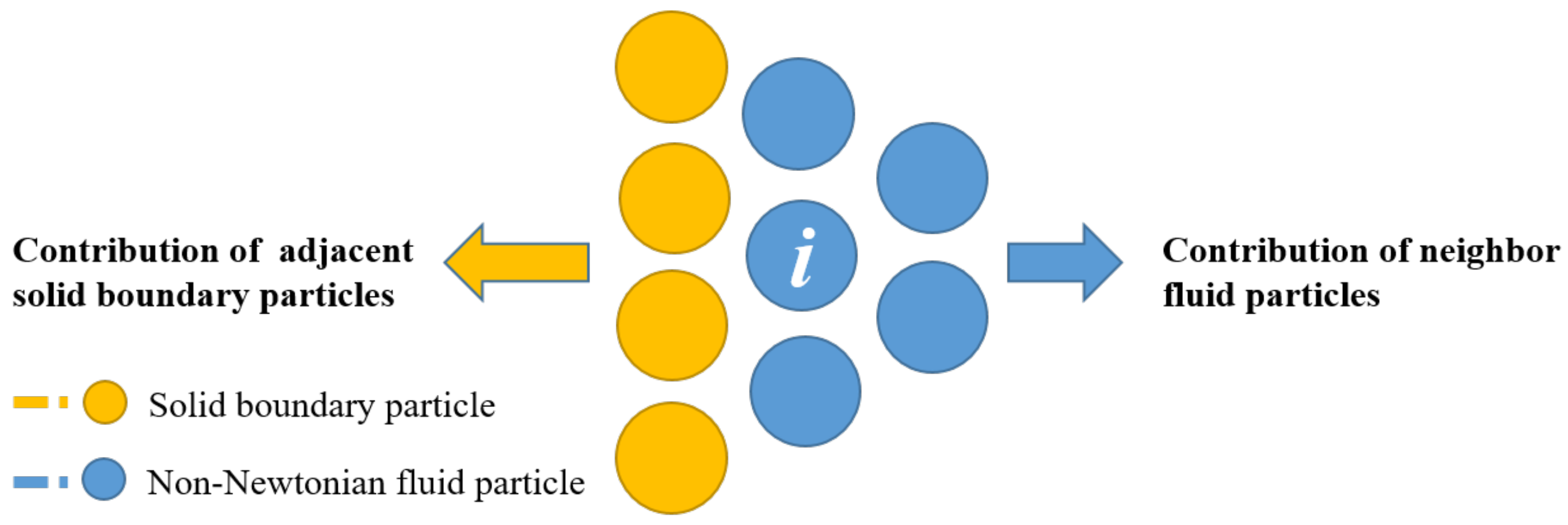
Figure 5.
The interaction forces among Non-Newtonian fluid and solid.

Figure 6.
Pouring water to a container. Upper row: Newtonian fluid. Lower row: non-Newtonian fluid.

Figure 7.
Friction boundary conditions of non-Newtonian fluid. Upper row: No friction boundary conditions. Lower row: Add friction boundary conditions.
Figure 7.
Friction boundary conditions of non-Newtonian fluid. Upper row: No friction boundary conditions. Lower row: Add friction boundary conditions.

Figure 8.
Fluid volume dropping on a planar solid object. Upper row: Newtonian fluid. Middle row: non-Newtonian fluid. Lower row: non-Newtonian fluid with our friction boundary condition.
Figure 8.
Fluid volume dropping on a planar solid object. Upper row: Newtonian fluid. Middle row: non-Newtonian fluid. Lower row: non-Newtonian fluid with our friction boundary condition.

Figure 9.
The stirring experiment of Non-Newtonian fluid.

Figure 10.
The melting butter in a plate.
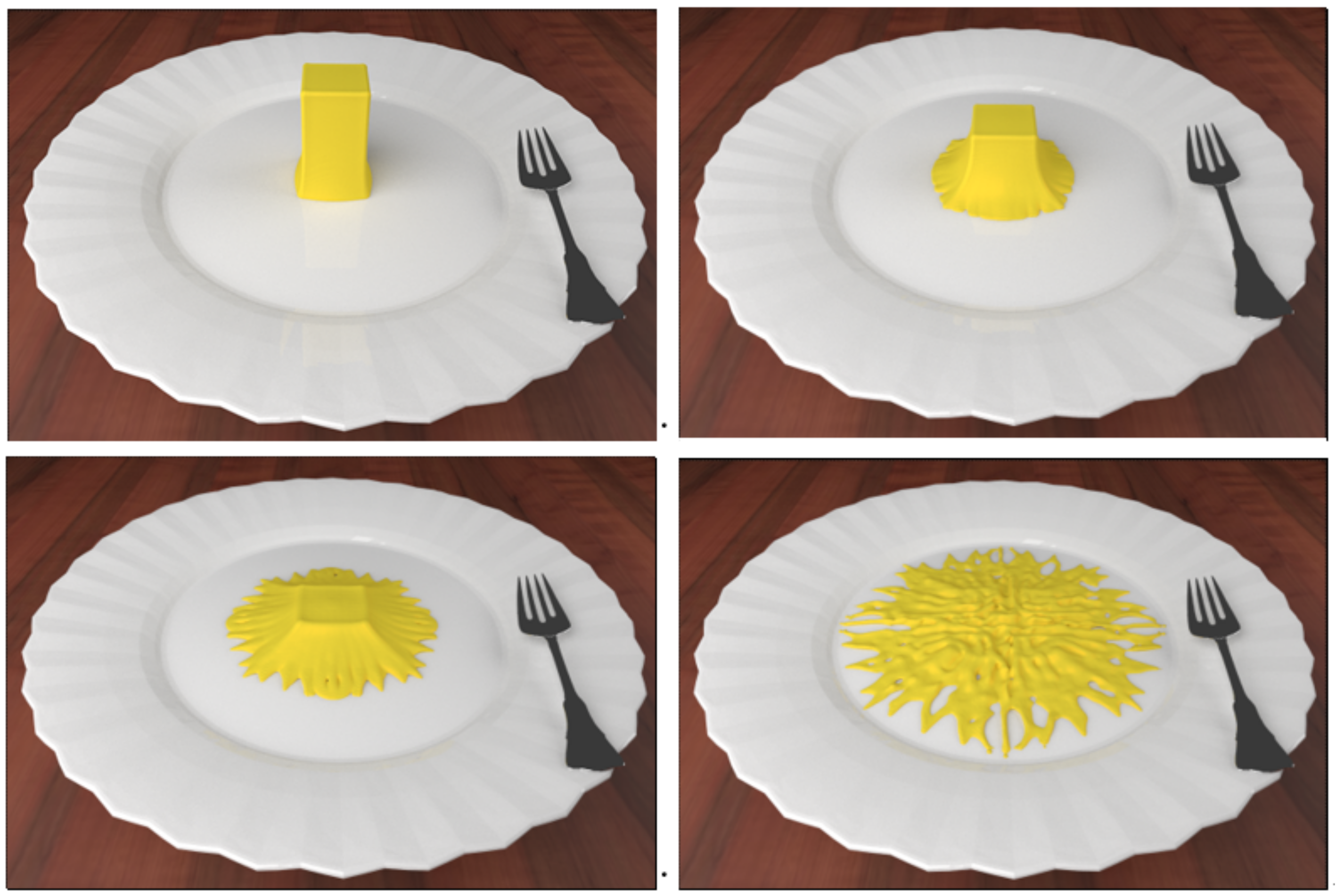
Figure 11.
Debris flow disaster simulation.

Table 1.
The parameters of the first three experiments.
| Item | Experiment 1 | Experiment 2 | Experiment 3 |
|---|---|---|---|
| Simulation domain size | 12 m × 12 m × 12 m | 20 m × 20 m × 20 m | 32 m × 30 m × 32 m |
| Smooth and kernel function | B- Spline function | B- Spline function | B- Spline function |
| Smooth radius | 0.2 m | 0.2 m | 0.3 m |
| Width of the fluid particles | 0.1 m | 0.1 m | 0.15 m |
| Number of fluid particles | 3.8 k | 13.67 k | 5.2 k |
| viscosity parameter I | 1 | 1 | 1 |
| viscosity parameter n | 0.5 | 0.5 | 0.5 |
| Upper limit of viscosity | 15 m/s | 2 m/s | 2 m/s |
| Lower limit of viscosity | 2 m/s | 0.2 m/s | 0.2 m/s |
| Total simulation time | 10 s | 20 s | 1.5 s |
Table 2.
The parameters of the last three experiments.
| Item | Experiment 4 | Experiment 5 | Experiment 6 |
|---|---|---|---|
| Simulation domain size | 12 m × 12 m × 12 m | 32 m × 30 m × 32 m | 40 m × 40 m × 40 m |
| Smooth and kernel function | B- Spline function | B- Spline function | B- Spline function |
| Smooth radius | 0.36 m | 0.3 m | 0.26 m |
| Width of the fluid particles | 0.18 m | 0.15 m | 0.13 m |
| Number of fluid particles | 32.7 k | 5.2 k | 57 k |
| viscosity parameter I | 1 | 1 | 1 |
| viscosity parameter n | 0.5 | 0.5 | 0.5 |
| Upper limit of viscosity | 2 m/s | 2 m/s | 2 m/s |
| Lower limit of viscosity | 0.2 m/s | 0.2 m/s | 0.2 m/s |
| Total simulation time | 15 s | 1.5 s | 20 s |
© 2018 by the authors. Licensee MDPI, Basel, Switzerland. This article is an open access article distributed under the terms and conditions of the Creative Commons Attribution (CC BY) license (http://creativecommons.org/licenses/by/4.0/).
Share and Cite
MDPI and ACS Style
Wang, X.; Ban, X.; He, R.; Wu, D.; Liu, X.; Xu, Y. Fluid-Solid Boundary Handling Using Pairwise Interaction Model for Non-Newtonian Fluid. Symmetry 2018, 10, 94. https://doi.org/10.3390/sym10040094
AMA Style
Wang X, Ban X, He R, Wu D, Liu X, Xu Y. Fluid-Solid Boundary Handling Using Pairwise Interaction Model for Non-Newtonian Fluid. Symmetry. 2018; 10(4):94. https://doi.org/10.3390/sym10040094
Chicago/Turabian StyleWang, Xiaokun, Xiaojuan Ban, Runzi He, Di Wu, Xing Liu, and Yuting Xu. 2018. "Fluid-Solid Boundary Handling Using Pairwise Interaction Model for Non-Newtonian Fluid" Symmetry 10, no. 4: 94. https://doi.org/10.3390/sym10040094
Note that from the first issue of 2016, this journal uses article numbers instead of page numbers. See further details here.