Generalized Interval Neutrosophic Choquet Aggregation Operators and Their Applications

Abstract

The interval neutrosophic set (INS) is a subclass of the neutrosophic set (NS) and a generalization of the interval-valued intuitionistic fuzzy set (IVIFS), which can be used in real engineering and scientific applications. This paper aims at developing new generalized Choquet aggregation operators for INSs, including the generalized interval neutrosophic Choquet ordered averaging (G-INCOA) operator and generalized interval neutrosophic Choquet ordered geometric (G-INCOG) operator. The main advantages of the proposed operators can be described as follows: (i) during decision-making or analyzing process, the positive interaction, negative interaction or non-interaction among attributes can be considered by the G-INCOA and G-INCOG operators; (ii) each generalized Choquet aggregation operator presents a unique comprehensive framework for INSs, which comprises a bunch of existing interval neutrosophic aggregation operators; (iii) new multi-attribute decision making (MADM) approaches for INSs are established based on these operators, and decision makers may determine the value of $\lambda$ by different MADM problems or their preferences, which makes the decision-making process more flexible; (iv) a new clustering algorithm for INSs are introduced based on the G-INCOA and G-INCOG operators, which proves that they have the potential to be applied to many new fields in the future.

1. Introduction

The neutrosophic set (NS) is a powerful comprehensive framework that comprises the concepts of the classic set, fuzzy set (FS), intuitionistic fuzzy set (IFS), hesitant fuzzy set (HFS), paraconsistent set, paradoxist set, and interval-valued fuzzy set (IVFS) [1,2,3,4]. It was introduced by Smarandache to deal with incomplete, indeterminate, and inconsistent decision information, which includes the truth membership, falsity membership, and indeterminacy membership, and their functions are non-standard subsets of $]{}^{-}0,1^{+}[$ [5]. However, without a specific description, it is difficult to apply the NS in practical application. Therefore, scholars proposed the interval neutrosophic set (INS), single-valued neutrosophic set (SVNS), rough neutrosophic set (RNS), multi-valued neutrosophic set (MVNS) as some special cases of the NS, and studied their related properties in [6,7,8,9]. Recently, numbers of new neutrosophic theories have been proposed and applied to image segmentation, image processing, rock mechanics, stock market, computational intelligence, multi-attribute decision making (MADM), medical diagnosis, fault diagnosis, and optimization design as described in [10,11,12,13].

The INS is a subclass of the NS and generalization of the IFS and IVIFS, which was proposed by Wang [6]. Motivated by some aggregation operators and decision-making methods for IFSs, IVIFSs, and NSs [14,15,16,17,18,19], a lot of theories about INSs have been put forward successively, and their basic concepts and aggregation tools play important roles in practical applications. For instance, Wang et al. [6] defined the basic operational relations for INSs and Zhang et al. [20] pointed out some drawbacks of these operational laws and improved them. Then they also put forward some basic aggregation operators to deal with MADM problems with interval neutrosophic information. Besides, Broumi [21] introduced the definition of correlation coefficient between INSs. Then Zhang et al. [22] pointed out some shortcomings of the existing correlation coefficient and they also proposed the definition of improved weighted correlation coefficient. Ye [23] defined some distance measures and similarity measures for INSs and applied these measures in practical MADM problems, and he also [24] proposed the interval neutrosophic ordered weighted arithmetic and geometric averaging operators, and further constructed a possibility degree ranking method under the interval neutrosophic environment. Moreover, Liu et al. [25,26,27] proposed the power generalized aggregation operators, the prioritized ordered weighted aggregation operators and induced generalized interval neutrosophic Shapley hybrid geometric averaging/mean operators for INSs under an interval neutrosophic environment.

For some practical problems, there exists mutual influence and interaction among attributes, which should be considered in decision-making or other analyzing process. The interaction between attributes can be classified into three types, which are positive interaction, negative interaction, and non-interaction [28,29]. Failure to consider the interactions among attributes may directly lead to errors of decision results. To solve this problem under the interval neutrosophic environment, we first intend to define some aggregation operators in this paper by combining the definition of Choquet integral to process the mutual influence and interaction among attributes with respect to fuzzy measure [30,31].

Besides, cluster analysis, or clustering, is defined as the unsupervised process of group (a set of data objects) in such a way that objects in the same group (called a cluster) are somehow more similar to each other than those in other groups (clusters) [32]. There are many algorithms for clustering which differ significantly in their notion of what constitutes a cluster and how to efficiently find them. Under a hesitant fuzzy environment, Chen et al. [33] proposed an algorithm to cluster hesitant fuzzy data into different clusters. Using the algorithm as a reference, we also intend to propose an effective new clustering algorithm under the interval neutrosophic environment.

Moreover, the generalized aggregation operators are a new class of operators, which have been widely applied in fuzzy areas, since they can be used to synthesize multi-dimensional evaluation values represented by kinds of hesitant fuzzy values or intuitionstic fuzzy values into collective values. Overall, this paper aims at proposing new generalized Choquet aggregation operators for INSs—namely, the G-INCOA operator and G-INCOG operator—which can be applied in MADM and clustering using interval neutrosophic information. In some special cases, each generalized aggregation operator reduces to various existing non-generalized interval neutrosophic aggregation operators.

To do so, the rest of this paper is organized as follows: Section 2 introduces some basic definitions about the Choquet integral and INS. In Section 3, the G-INCOA operator and G-INCOG operator are put forward and some desirable properties of them are discussed and proved. We also consider special cases of these operators and distinguish them in two main classes, the first class focuses on the parameter $\lambda$, and the second class on the fuzzy measure $\mu \left(x_j\right)$. In Section 4, we put forward some novel MADM methods based on the proposed operators to deal with interval neutrosophic information and utilize an illustrative example to validate the proposed MADM approaches by taking different values of parameter $\lambda$ of the proposed operators. In Section 5, a new clustering algorithm for INSs is introduced based on the G-INCOA operator and the G-INCOG operator. Then, a numerical example concerning clustering is utilized as the demonstration of the application and effectiveness of the proposed clustering algorithm. Finally, conclusions and future research directions are drawn in Section 6.

2. Preliminaries

To facilitate the following discussion, some basic definitions about the Choquet integral and INS are briefly introduced in this section.

2.1. Interval Neutrosophic Sets (INS)

The NS was firstly introduced by Smarandache [5], which is a comprehensive framework for expressing and processing incomplete and indeterminate information.

Definition 1.

([5]) Let X be a non-empty fixed set, a NS on X is defined as:

$$\begin{array}{c}{T}_A\left(x\right),I_A\left(x\right),F_A\left(x\right):X\to ]{}^{-}0,1^{+}[,\end{array}$$

(1)

where $T_A\left(x\right),I_A\left(x\right),F_A\left(x\right)$ representing the truth membership function, indeterminacy membership function and falsity membership function, respectively, and satisfying the limit: $0^{-}\le sup{T}_A\left(x\right)+sup{I}_A\left(x\right)+sup{F}_A\left(x\right)\le 3^{+}.$

It is not difficult to find that the NS is difficult to apply in the real applications. Therefore, Wang et al. [6] proposed the interval neutrosophic set (INS) as an instance of the NS, which is defined as:

Definition 2.

([6]) Let X be a non-empty finite set, an INS in X is expressed by:

$$\begin{array}{c}N=\{\langle x,[{\tilde{t}}^L\left(x\right),{\tilde{t}}^U\left(x\right)],[{\tilde{i}}^L\left(x\right),{\tilde{i}}^U\left(x\right)],[{\tilde{f}}^L\left(x\right),{\tilde{f}}^U\left(x\right)\rangle ]|x\in X\},\end{array}$$

(2)

where $\tilde{t}\left(x\right)=[{\tilde{t}}^L\left(x\right),{\tilde{t}}^U\left(x\right)]\subseteq [0,1],\tilde{i}\left(x\right)=[{\tilde{i}}^L\left(x\right),{\tilde{i}}^U\left(x\right)]\subseteq [0,1],$ $\tilde{f}\left(x\right)=[{\tilde{f}}^L\left(x\right),{\tilde{f}}^U\left(x\right)]\subseteq [0,1]$ representing truth, indeterminacy, and falsity membership functions of the element $x\in X$, and satisfying limits:$0\le {\tilde{t}}^U\left(x\right)+{\tilde{i}}^U\left(x\right)+{\tilde{f}}^U\left(x\right)\le 3$.

For convenience, we call $\tilde{n}=\langle [{\tilde{t}}^L,{\tilde{t}}^U],[{\tilde{i}}^L,{\tilde{i}}^U],[{\tilde{f}}^L,{\tilde{f}}^U]\rangle$ an interval neutrosophic element (INN). The basic operational relations of INNs are defined as:

Definition 3.

([6]) Let $\widetilde{n_1}=\langle [{\tilde{t}}_1^L,{\tilde{t}}_1^U],[{\tilde{i}}_1^L,{\tilde{i}}_1^U],[{\tilde{f}}_1^U,{\tilde{f}}_1^U]\rangle$ and $\widetilde{n_2}=\langle [{\tilde{t}}_2^L,{\tilde{t}}_2^U],[{\tilde{i}}_2^L,{\tilde{i}}_2^U],[{\tilde{f}}_2^U,{\tilde{f}}_2^U]\rangle$ be two INNs, then:

• $\widetilde{n_1}\oplus \widetilde{n_2}=\langle [{\tilde{t}}_1^L+{\tilde{t}}_2^L-{\tilde{t}}_1^L{\tilde{t}}_2^L,{\tilde{t}}_1^U+{\tilde{t}}_2^U-{\tilde{t}}_1^U{\tilde{t}}_2^U],[{\tilde{i}}_1^L{\tilde{i}}_2^L,{\tilde{i}}_1^U{\tilde{i}}_2^U],[{\tilde{f}}_1^L{\tilde{f}}_2^L,{\tilde{f}}_1^U{\tilde{f}}_2^U]\rangle ;$
• $\widetilde{n_1}\oplus \widetilde{n_2}=\langle [{\tilde{t}}_1^L{\tilde{t}}_2^L,{\tilde{t}}_1^U{\tilde{t}}_2^U],[{\tilde{i}}_1^L+{\tilde{i}}_2^L-{\tilde{i}}_1^L{\tilde{i}}_2^L,{\tilde{i}}_1^U+{\tilde{i}}_2^U-{\tilde{i}}_1^U{\tilde{i}}_2^U],[{\tilde{f}}_1^L+{\tilde{f}}_2^L-{\tilde{f}}_1^L{\tilde{i}}_2^L,{\tilde{f}}_1^U+{\tilde{f}}_2^U-{\tilde{f}}_1^U{\tilde{f}}_2^U]\rangle ;$
• $r\widetilde{n_1}=\langle [1-{(1-{\tilde{t}}_1^L)}^r,1-{(1-{\tilde{t}}_1^U)}^r],[{({\tilde{i}}_1^L)}^r,{({\tilde{i}}_1^U)}^r],[{({\tilde{f}}_1^L)}^r,{({\tilde{f}}_1^U)}^r]\rangle$;
• ${\widetilde{n_1}}^r=\langle [{({\tilde{t}}_1^L)}^r,{({\tilde{t}}_1^U)}^r],[1-{(1-{\tilde{i}}_1^L)}^r,1-{(1-{\tilde{i}}_1^U)}^r],[1-{(1-{\tilde{f}}_1^L)}^r,1-{(1-{\tilde{f}}_1^U)}^r]\rangle$.

2.2. Some Concepts of INSs

On the basis of the distance measures of INSs [23], Ye defined some similarity measures between INSs $\widetilde{n_1}$ and $\widetilde{n_2}$, which can be given as:

Definition 4.

Let $\widetilde{n_1}=\langle [{\tilde{t}}_1^L,{\tilde{t}}_1^U],[{\tilde{i}}_1^L,{\tilde{i}}_1^U],[{\tilde{f}}_1^U,{\tilde{f}}_1^U]\rangle$ and $\widetilde{n_2}=\langle [{\tilde{t}}_2^L,{\tilde{t}}_2^U],[{\tilde{i}}_2^L,{\tilde{i}}_2^U],[{\tilde{f}}_2^U,{\tilde{f}}_2^U]\rangle$ be two INNs, thus, the similarity function between $\widetilde{n_1}$ and $\widetilde{n_2}$ is defined by:

$$\begin{array}{c}C\left(\widetilde{n_1},\widetilde{n_2}\right)=1-\frac{\left({\left({\tilde{t}}_1^L-{\tilde{t}}_2^L\right)}^2+{\left({\tilde{i}}_1^L-{\tilde{i}}_2^L\right)}^2+{\left({\tilde{f}}_1^L-{\tilde{f}}_2^L\right)}^2+{\left({\tilde{t}}_1^U-{\tilde{t}}_2^U\right)}^2+{\left({\tilde{i}}_1^U-{\tilde{i}}_2^U\right)}^2+{\left({\tilde{f}}_1^U-{\tilde{f}}_2^U\right)}^2\right)}{6}.\end{array}$$

(3)

According to the value range of the similarity measures, we can obtain the value range of the cosine function, we can obtain the following property $0\le C\left(\widetilde{n_1},\widetilde{n_2}\right)\le 1$. Suppose the best ideal alternative ${\tilde{n}}^{+}=\langle [{{\tilde{t}}_1^L}^{+},{{\tilde{t}}_1^U}^{+}],[{{\tilde{i}}_1^L}^{+},{{\tilde{i}}_1^U}^{+}],[{{\tilde{f}}_1^L}^{+},{{\tilde{f}}_1^U}^{+}]\rangle =\langle [1,1],[0,0],[0,0]\rangle$, then, the similarity measures between $\widetilde{n_1}$ and ${\tilde{n}}^{+}$ can be described as:

$$\begin{array}{c}C\left(\widetilde{n_1},\widetilde{n_2}\right)=1-\frac{\left({\left(1-{\tilde{t}}_1^L\right)}^2+{\left({\tilde{i}}_1^L\right)}^2+{\left({\tilde{f}}_1^L\right)}^2+{\left(1-{\tilde{t}}_1^U\right)}^2+{\left({\tilde{i}}_1^U\right)}^2+{\left({\tilde{f}}_1^U\right)}^2\right)}{6}.\end{array}$$

(4)

The score function are effective tools to rank INNs, and here we give its definition:

Definition 5.

([25]) For $\tilde{n}$, the score function $s\left(\tilde{n}\right)$ is defined as:

$$\begin{array}{c}s\left(\tilde{n}\right)=\left(\frac{\left({\tilde{t}}_1^L+{\tilde{t}}_1^U\right)}{2}+\left(1-\frac{\left({\tilde{i}}_1^L+{\tilde{i}}_1^U\right)}{2}\right)+\left(1-\frac{\left({\tilde{f}}_1^L+{\tilde{f}}_1^U\right)}{2}\right)\right)/3\end{array}$$

(5)

obviously,$s\left(\tilde{n}\right)\in [0,1]$. If$s\left({\tilde{n}}_1\right)>s\left({\tilde{n}}_2\right)$, then ${\tilde{n}}_1>{\tilde{n}}_2$.

2.3. The Fuzzy Measure and Choquet Integral

The Choquet integral is a powerful operator to aggregate kinds of fuzzy information in MADM with respect to fuzzy measure.

Definition 6.

([30]) Let $\left(X,\mathcal{A},\mu \right)$ be a measurable space and $\mu :\mathcal{A}\to [0,1]$, if it satisfies the conditions:

• $\mu (\varnothing )=0;$
• $\mu \left(A\right)\le \mu \left(B\right)\mathrm{whenever}A\subset B,A,B\in \mathcal{A};$
• $If{A}_1\subset A_2\subset \dots \subset A_n\subset \dots ,A_n\in \mathcal{A},\mathrm{then}\mu \left({{\displaystyle \cup }}_{n=1}^{\infty }{A}_n\right)=li{m}_{n\to \infty }\mu \left(A_n\right);$
• $If{A}_1\supset A_2\supset \dots \supset A_n\supset \dots ,A_n\in \mathcal{A},\mathrm{then}\mu \left({{\displaystyle \cup }}_{n=1}^{\infty }{A}_n\right)=li{m}_{n\to \infty }\mu \left(A_n\right);$

then, we call $\mathsf{\mu }$ be a fuzzy measure defined by Sugeno M.

To avoid the problems with computational complexity in paractical applications, $g_{\lambda }$ fuzzy measure also called $\lambda$-fuzzy measure, was proposed by Sugeno M [30], which satisfies an additional properties:$\mu \left(X{\displaystyle \cup }Y\right)=\mu \left(X\right)+\mu \left(Y\right)+g_{\lambda }\mu \left(X\right)\mu \left(Y\right),g_{\lambda }\in \left(-1,\infty \right)$ for all $X,Y\in \mathcal{A}$ and $X{\displaystyle \cap }Y=\varnothing$. Specially, the expression of $g_{\lambda }$ fuzzy measure defined on a finite set X = {$x_1,x_2,\dots ,x_m$} can be simplified as:

Theorem 1.

([30]) Let X be a set (X = {$x_1,x_2,\dots ,x_m$}), $\lambda$-fuzzy measure defined on X is expressed as:

$$\begin{array}{c}\mu \left(X\right)=\{\begin{array}{c}\frac{1}{{\mathsf{\lambda }}_g}\left({\displaystyle \prod _{i\in X}}\left(1+{\mathsf{\lambda }}_g\mu \left(x_i\right)\right)-1\right),if{\mathsf{\lambda }}_g\ne 0,\\ {\displaystyle \sum _{i\in X}}\mu \left(x_i\right),if{\mathsf{\lambda }}_g=0,\end{array}\end{array}$$

(6)

where $x_i{\displaystyle \cap }{x}_j=\varnothing$ for all $i,j=1,2,3,\dots ,m$ and $i\ne j$.

Then, the Choquet integral with respect to fuzzy measures, is defined as:

Definition 7.

([31]) When $\mathsf{\mu }$ is a fuzzy measure, X = {$x_1,x_2,\dots ,x_m$} is a finite set. The Choquet integral of a function $f:X\to [0,1]$ with respect to fuzzy measure $\mathsf{\mu }$ can be expressed as:

$$\begin{array}{c}{\displaystyle \int }fd\mu ={\displaystyle \sum _{i=1}^m}\left(\mu \left(F_{\varphi \left(i\right)}\right)-\mu \left(F_{\varphi \left(i-1\right)}\right)\right)\oplus f\left(x_{\varphi \left(i\right)}\right),\end{array}$$

(7)

where $\left(\varphi \left(1\right),\varphi \left(2\right),\dots \varphi \left(i\right),\dots ,\varphi \left(m\right)\right)$ is a permutation of $\left(1,2,\dots i,\dots ,m\right)$ such that $f\left(x_{\varphi \left(1\right)}\right)\le f\left(x_{\varphi \left(2\right)}\right)\le ,\dots ,\le f\left(x_{\varphi \left(i\right)}\right)\le ,\dots ,\le f\left(x_{\varphi \left(m\right)}\right),$ $F_{\varphi \left(i\right)}=\{x_{\varphi \left(1\right)},x_{\varphi \left(2\right)},\dots ,x_{\varphi \left(i\right)}\}$ and $F_{\varphi \left(0\right)}=\varnothing .$

3. Generalized Interval Neutrosphic Choquet Aggregation Operators

In what follows, based on the operational relations of INNs and Choquet aggregation operator, we shall develop new generalized Choquet aggregation operators under the interval neutrosophic environment, such as the generalized interval neutrosophic Choquet ordered averaging (G-INCOA) operator and generalized interval neutrosophic Choquet ordered geometric (G-INCOG) operator.

3.1. The G-INCOA and G-INCOG Operators

Definition 8.

When ${\tilde{n}}_j\left(j=1,2,3,\dots ,m\right)$ is a collection of INNs, X= {$x_1,x_2,x_3,\dots ,x_m$} is the set of attributes and $\mu$ measure on X, the G-INCOA and G-INCOG operators are defined as:

$$\begin{array}{c}G-INCO{A}_{\mu ,\lambda }\{{\tilde{n}}_1,{\tilde{n}}_2,\dots ,{\tilde{n}}_m\}={\left({\oplus }_{j=1}^m\left(\mu \left(F_{\varphi \left(j\right)}\right)-\mu \left(F_{\varphi \left(j-1\right)}\right)\right){\tilde{n}}_{\varphi \left(j\right)}{}^{\lambda }\right)}^{\frac{1}{\lambda }},\end{array}$$

(8)

$$\begin{array}{c}G-INCO{G}_{\mu ,\lambda }\{{\tilde{n}}_1,{\tilde{n}}_2,\dots ,{\tilde{n}}_m\}={\left({\otimes }_{j=1}^m\left(\mu \left(F_{\varphi \left(j\right)}\right)-\mu \left(F_{\varphi \left(j-1\right)}\right)\right){\tilde{n}}_{\varphi \left(j\right)}{}^{\lambda }\right)}^{\frac{1}{\lambda }},\end{array}$$

(9)

where $\lambda >0,{\mu }_{\varphi \left(i\right)}=\mu \left(F_{\varphi \left(i\right)}\right)-\mu \left(F_{\varphi \left(i-1\right)}\right)$. where $\left(\varphi \left(1\right),\varphi \left(2\right),\dots \varphi \left(i\right),\dots ,\varphi \left(m\right)\right)$ is a permutation of $\left(1,2,\dots i,\dots ,m\right)$ such that $f\left(x_{\varphi \left(1\right)}\right)\le f\left(x_{\varphi \left(2\right)}\right)\le ,\dots ,\le f\left(x_{\varphi \left(i\right)}\right)\le ,\dots ,\le f\left(x_{\varphi \left(m\right)}\right),F_{\varphi \left(0\right)}=\varnothing$ and $F_{\varphi \left(i\right)}=\{x_{\varphi \left(1\right)},x_{\varphi \left(2\right)},\dots ,x_{\varphi \left(i\right)}\}.$

Theorem 2.

When ${\tilde{n}}_j\left(j=1,2,3,\dots ,m\right)$ is a collection of INNs, then the aggregated value obtained by the G-INCOA operator is also a INN, and:

$$\begin{gathered} G-INCO{A}_{\mu ,\lambda }\{{\tilde{n}}_1,{\tilde{n}}_2,\dots ,{\tilde{n}}_m\}={\left({\oplus }_{j=1}^m\left(\mu \left(F_{\varphi \left(j\right)}\right)-\mu \left(F_{\varphi \left(j-1\right)}\right)\right){\tilde{n}}_{\varphi \left(j\right)}{}^{\lambda }\right)}^{\frac{1}{\lambda }} \\ =\{\left[{\left(1-{\displaystyle \prod }_{j=1}^m{\left(1-{\left(t_{\varphi \left(j\right)}^L\right)}^{\lambda }\right)}^{{\mu }_{\varphi \left(j\right)}}\right)}^{\frac{1}{\lambda }},{\left(1-{\displaystyle \prod }_{j=1}^m{\left(1-{\left(t_{\varphi \left(j\right)}^U\right)}^{\lambda }\right)}^{{\mu }_{\varphi \left(j\right)}}\right)}^{\frac{1}{\lambda }}\right], \\ \left[1-{\left(1-{\displaystyle \prod }_{j=1}^m{\left(1-{\left(1-i_{\varphi \left(j\right)}^L\right)}^{\lambda }\right)}^{{\mu }_{\varphi \left(j\right)}}\right)}^{\frac{1}{\lambda }},1-{\left(1-{\displaystyle \prod }_{j=1}^m{\left(1-{\left(1-i_{\varphi \left(j\right)}^U\right)}^{\lambda }\right)}^{{\mu }_{\varphi \left(j\right)}}\right)}^{\frac{1}{\lambda }}\right], \\ \left[1-{\left(1-{\displaystyle \prod }_{j=1}^m{\left(1-{\left(1-f_{\varphi \left(j\right)}^L\right)}^{\lambda }\right)}^{{\mu }_{\varphi \left(j\right)}}\right)}^{\frac{1}{\lambda }},1-{\left(1-{\displaystyle \prod }_{j=1}^m{\left(1-{\left(1-f_{\varphi \left(j\right)}^U\right)}^{\lambda }\right)}^{{\mu }_{\varphi \left(j\right)}}\right)}^{\frac{1}{\lambda }}\right]\}. \end{gathered}$$

(10)

Similarly, the aggregated value obtained by the G-INCOG operator is also a INN,

$$\begin{gathered} G-INCO{G}_{\mu ,\lambda }\{{\tilde{n}}_1,{\tilde{n}}_2,\dots ,{\tilde{n}}_m\}={\left({\oplus }_{j=1}^m\left(\mu \left(F_{\varphi \left(j\right)}\right)-\mu \left(F_{\varphi \left(j-1\right)}\right)\right){\tilde{n}}_{\varphi \left(j\right)}{}^{\lambda }\right)}^{\frac{1}{\lambda }}, \\ =\{\left[1-{\left(1-{\displaystyle \prod }_{j=1}^m{\left(1-{\left(1-t_{\varphi \left(j\right)}^L\right)}^{\lambda }\right)}^{{\mu }_{\varphi \left(j\right)}}\right)}^{\frac{1}{\lambda }},1-{\left(1-{\displaystyle \prod }_{j=1}^m{\left(1-{\left(1-t_{\varphi \left(j\right)}^U\right)}^{\lambda }\right)}^{{\mu }_{\varphi \left(j\right)}}\right)}^{\frac{1}{\lambda }}\right], \\ \left[{\left(1-{\displaystyle \prod }_{j=1}^m{\left(1-{\left(i_{\varphi \left(j\right)}^L\right)}^{\lambda }\right)}^{{\mu }_{\varphi \left(j\right)}}\right)}^{\frac{1}{\lambda }},{\left(1-{\displaystyle \prod }_{j=1}^m{\left(1-{\left(i_{\varphi \left(j\right)}^U\right)}^{\lambda }\right)}^{{\mu }_{\varphi \left(j\right)}}\right)}^{\frac{1}{\lambda }}\right], \\ \left[{\left(1-{\displaystyle \prod }_{j=1}^m{\left(1-{\left(f_{\varphi \left(j\right)}^L\right)}^{\lambda }\right)}^{{\mu }_{\varphi \left(j\right)}}\right)}^{\frac{1}{\lambda }},{\left(1-{\displaystyle \prod }_{j=1}^m{\left(1-{\left(f_{\varphi \left(j\right)}^U\right)}^{\lambda }\right)}^{{\mu }_{\varphi \left(j\right)}}\right)}^{\frac{1}{\lambda }}\right]\}. \end{gathered}$$

(11)

Proof. 

The result of $m=1$ follows quickly from Definition 8, below we prove Equations (10) and (11) by means of mathematical induction on m, here, take Equation (11) as an example.

(a) For $m=2,$ based on the operation relations of INNs defined in Definition 3, we have:

$$\begin{gathered} {\left({\mu }_{\varphi \left(1\right)}{\tilde{n}}_{\varphi \left(1\right)}{}^{\lambda }\right)}^{\frac{1}{\lambda }}=\{\left[1-{\left(1-{\left(1-{\left(1-t_{\varphi \left(1\right)}^L\right)}^{\lambda }\right)}^{{\mu }_{\varphi \left(1\right)}}\right)}^{\frac{1}{\lambda }},1-{\left(1-{\left(1-{\left(1-t_{\varphi \left(1\right)}^U\right)}^{\lambda }\right)}^{{\mu }_{\varphi \left(1\right)}}\right)}^{\frac{1}{\lambda }}\right], \\ \left[{\left(1-{\left(1-{\left(i_{\varphi \left(1\right)}^L\right)}^{\lambda }\right)}^{{\mu }_{\varphi \left(1\right)}}\right)}^{\frac{1}{\lambda }},{\left(1-{\left(1-{\left(i_{\varphi \left(1\right)}^U\right)}^{\lambda }\right)}^{{\mu }_{\varphi \left(1\right)}}\right)}^{\frac{1}{\lambda }}\right],\left[{\left(1-{\left(1-{\left(f_{\varphi \left(1\right)}^L\right)}^{\lambda }\right)}^{{\mu }_{\varphi \left(1\right)}}\right)}^{\frac{1}{\lambda }},{\left(1-{\left(1-{\left(f_{\varphi \left(1\right)}^U\right)}^{\lambda }\right)}^{{\mu }_{\varphi \left(1\right)}}\right)}^{\frac{1}{\lambda }}\right]\}; \end{gathered}$$

$$\begin{gathered} {\left({\mu }_{\varphi \left(2\right)}{\tilde{n}}_{\varphi \left(2\right)}{}^{\lambda }\right)}^{\frac{1}{\lambda }}=\{\left[1-{\left(1-{\left(1-{\left(1-t_{\varphi \left(2\right)}^L\right)}^{\lambda }\right)}^{{\mu }_{\varphi \left(2\right)}}\right)}^{\frac{1}{\lambda }},1-{\left(1-{\left(1-{\left(1-t_{\varphi \left(2\right)}^U\right)}^{\lambda }\right)}^{{\mu }_{\varphi \left(2\right)}}\right)}^{\frac{1}{\lambda }}\right], \\ \left[{\left(1-{\left(1-{\left(i_{\varphi \left(2\right)}^L\right)}^{\lambda }\right)}^{{\mu }_{\varphi \left(2\right)}}\right)}^{\frac{1}{\lambda }},{\left(1-{\left(1-{\left(i_{\varphi \left(2\right)}^U\right)}^{\lambda }\right)}^{{\mu }_{\varphi \left(2\right)}}\right)}^{\frac{1}{\lambda }}\right],\left[{\left(1-{\left(1-{\left(f_{\varphi \left(2\right)}^L\right)}^{\lambda }\right)}^{{\mu }_{\varphi \left(2\right)}}\right)}^{\frac{1}{\lambda }},{\left(1-{\left(1-{\left(f_{\varphi \left(2\right)}^U\right)}^{\lambda }\right)}^{{\mu }_{\varphi \left(2\right)}}\right)}^{\frac{1}{\lambda }}\right]\}; \end{gathered}$$

thus, for $m=2,$ the $G-INCO{G}_{\mu ,\lambda }\{{\tilde{n}}_1,{\tilde{n}}_2\}$ can be obtained as:

$$\begin{gathered} G-INCO{G}_{\mu ,\lambda }\{{\tilde{n}}_1,{\tilde{n}}_2\}={\left({\mu }_{\varphi \left(1\right)}{\tilde{n}}_{\varphi \left(1\right)}{}^{\lambda }\right)}^{\frac{1}{\lambda }}\oplus {\left({\mu }_{\varphi \left(2\right)}{\tilde{n}}_{\varphi \left(2\right)}{}^{\lambda }\right)}^{\frac{1}{\lambda }}= \\ \{\left[1-{\left(1-{\left(1-{\left(1-t_{\varphi \left(1\right)}^L\right)}^{\lambda }\right)}^{{\mu }_{\varphi \left(1\right)}}{\left(1-{\left(1-t_{\varphi \left(2\right)}^L\right)}^{\lambda }\right)}^{{\mu }_{\varphi \left(2\right)}}\right)}^{\frac{1}{\lambda }},1-{\left(1-{\left(1-{\left(1-t_{\varphi \left(1\right)}^U\right)}^{\lambda }\right)}^{{\mu }_{\varphi \left(1\right)}}{\left(1-{\left(1-t_{\varphi \left(2\right)}^U\right)}^{\lambda }\right)}^{{\mu }_{\varphi \left(2\right)}}\right)}^{\frac{1}{\lambda }}\right], \\ \left[{\left(1-{\left(1-{\left(i_{\varphi \left(1\right)}^L\right)}^{\lambda }\right)}^{{\mu }_{\varphi \left(1\right)}}{\left(1-{\left(i_{\varphi \left(2\right)}^L\right)}^{\lambda }\right)}^{{\mu }_{\varphi \left(2\right)}}\right)}^{\frac{1}{\lambda }},{\left(1-{\left(1-{\left(i_{\varphi \left(1\right)}^U\right)}^{\lambda }\right)}^{{\mu }_{\varphi \left(1\right)}}{\left(1-{\left(i_{\varphi \left(2\right)}^U\right)}^{\lambda }\right)}^{{\mu }_{\varphi \left(2\right)}}\right)}^{\frac{1}{\lambda }}\right], \\ \left[{\left(1-{\left(1-{\left(f_{\varphi \left(1\right)}^L\right)}^{\lambda }\right)}^{{\mu }_{\varphi \left(1\right)}}{\left(1-{\left(f_{\varphi \left(2\right)}^L\right)}^{\lambda }\right)}^{{\mu }_{\varphi \left(2\right)}}\right)}^{\frac{1}{\lambda }},{\left(1-{\left(1-{\left(f_{\varphi \left(1\right)}^U\right)}^{\lambda }\right)}^{{\mu }_{\varphi \left(1\right)}}{\left(1-{\left(f_{\varphi \left(2\right)}^U\right)}^{\lambda }\right)}^{{\mu }_{\varphi \left(2\right)}}\right)}^{\frac{1}{\lambda }}\right]\}, \end{gathered}$$

thus, Equation (11) holds for $m=2$.

(b) If Equation (11) holds for $m=k$, then:

$$\begin{gathered} G-INCO{G}_{\mu ,\lambda }\{{\tilde{n}}_1,{\tilde{n}}_2,\dots ,{\tilde{n}}_k\}=\{\left[1-{\left(1-{\displaystyle \prod }_{j=1}^k{\left(1-{\left(1-t_{\varphi \left(j\right)}^L\right)}^{\lambda }\right)}^{{\mu }_{\varphi \left(j\right)}}\right)}^{\frac{1}{\lambda }},1-{\left(1-{\displaystyle \prod }_{j=1}^k{\left(1-{\left(1-t_{\varphi \left(j\right)}^U\right)}^{\lambda }\right)}^{{\mu }_{\varphi \left(j\right)}}\right)}^{\frac{1}{\lambda }}\right], \\ \left[{\left(1-{\displaystyle \prod }_{j=1}^k{\left(1-{\left(i_{\varphi \left(j\right)}^L\right)}^{\lambda }\right)}^{{\mu }_{\varphi \left(j\right)}}\right)}^{\frac{1}{\lambda }},{\left(1-{\displaystyle \prod }_{j=1}^k{\left(1-{\left(i_{\varphi \left(j\right)}^U\right)}^{\lambda }\right)}^{{\mu }_{\varphi \left(j\right)}}\right)}^{\frac{1}{\lambda }}\right], \\ \left[{\left(1-{{\displaystyle \prod }}_{j=1}^k{\left(1-{\left(f_{\varphi \left(j\right)}^L\right)}^{\lambda }\right)}^{{\mu }_{\varphi \left(j\right)}}\right)}^{\frac{1}{\lambda }},{\left(1-{{\displaystyle \prod }}_{j=1}^k{\left(1-{\left(f_{\varphi \left(j\right)}^U\right)}^{\lambda }\right)}^{{\mu }_{\varphi \left(j\right)}}\right)}^{\frac{1}{\lambda }}\right]\}. \end{gathered}$$

For $m=k+1,$

$$\begin{gathered} G-INCO{G}_{\mu ,\lambda }\{{\tilde{n}}_1,{\tilde{n}}_2,\dots ,{\tilde{n}}_k,{\tilde{n}}_{k+1}\}={\left({\oplus }_{j=1}^k\left(\mu \left(F_{\varphi \left(j\right)}\right)-\mu \left(F_{\varphi \left(j-1\right)}\right)\right){\tilde{n}}_{\varphi \left(j\right)}{}^{\lambda }\right)}^{\frac{1}{\lambda }}\oplus {\left({\mu }_{\varphi \left(k+1\right)}{\tilde{n}}_{\varphi \left(k+1\right)}{}^{\lambda }\right)}^{\frac{1}{\lambda }}= \\ \{\left[1-{\left(1-{\displaystyle \prod }_{j=1}^k{\left(1-{\left(1-t_{\varphi \left(j\right)}^L\right)}^{\lambda }\right)}^{{\mu }_{\varphi \left(j\right)}}\right)}^{\frac{1}{\lambda }},1-{\left(1-{\displaystyle \prod }_{j=1}^k{\left(1-{\left(1-t_{\varphi \left(j\right)}^U\right)}^{\lambda }\right)}^{{\mu }_{\varphi \left(j\right)}}\right)}^{\frac{1}{\lambda }}\right], \\ \left[{\left(1-{\displaystyle \prod }_{j=1}^k{\left(1-{\left(i_{\varphi \left(j\right)}^L\right)}^{\lambda }\right)}^{{\mu }_{\varphi \left(j\right)}}\right)}^{\frac{1}{\lambda }},{\left(1-{\displaystyle \prod }_{j=1}^k{\left(1-{\left(i_{\varphi \left(j\right)}^U\right)}^{\lambda }\right)}^{{\mu }_{\varphi \left(j\right)}}\right)}^{\frac{1}{\lambda }}\right], \\ \left[{\left(1-{\displaystyle \prod }_{j=1}^k{\left(1-{\left(f_{\varphi \left(j\right)}^L\right)}^{\lambda }\right)}^{{\mu }_{\varphi \left(j\right)}}\right)}^{\frac{1}{\lambda }},{\left(1-{\displaystyle \prod }_{j=1}^k{\left(1-{\left(f_{\varphi \left(j\right)}^U\right)}^{\lambda }\right)}^{{\mu }_{\varphi \left(j\right)}}\right)}^{\frac{1}{\lambda }}\right]\}\otimes \\ \{\left[1-{\left(1-{\left(1-{\left(1-t_{\varphi \left(k+1\right)}^L\right)}^{\lambda }\right)}^{{\mu }_{\varphi \left(k+1\right)}}\right)}^{\frac{1}{\lambda }},1-{\left(1-{\left(1-{\left(1-t_{\varphi \left(k+1\right)}^U\right)}^{\lambda }\right)}^{{\mu }_{\varphi \left(k+1\right)}}\right)}^{\frac{1}{\lambda }}\right], \\ \left[{\left(1-{\left(1-{\left(i_{\varphi \left(k+1\right)}^L\right)}^{\lambda }\right)}^{{\mu }_{\varphi \left(k+1\right)}}\right)}^{\frac{1}{\lambda }},{\left(1-{\left(1-{\left(i_{\varphi \left(k+1\right)}^U\right)}^{\lambda }\right)}^{{\mu }_{\varphi \left(k+1\right)}}\right)}^{\frac{1}{\lambda }}\right] \\ \left[{\left(1-{\left(1-{\left(f_{\varphi \left(k+1\right)}^L\right)}^{\lambda }\right)}^{{\mu }_{\varphi \left(k+1\right)}}\right)}^{\frac{1}{\lambda }},{\left(1-{\left(1-{\left(f_{\varphi \left(k+1\right)}^U\right)}^{\lambda }\right)}^{{\mu }_{\varphi \left(k+1\right)}}\right)}^{\frac{1}{\lambda }}\right]\} \\ =\{\left[1-{\left(1-{\displaystyle \prod }_{j=1}^{k+1}{\left(1-{\left(1-t_{\varphi \left(j\right)}^L\right)}^{\lambda }\right)}^{{\mu }_{\varphi \left(j\right)}}\right)}^{\frac{1}{\lambda }},1-{\left(1-{\displaystyle \prod }_{j=1}^{k+1}{\left(1-{\left(1-t_{\varphi \left(j\right)}^U\right)}^{\lambda }\right)}^{{\mu }_{\varphi \left(j\right)}}\right)}^{\frac{1}{\lambda }}\right], \\ \left[{\left(1-{\displaystyle \prod }_{j=1}^{k+1}{\left(1-{\left(i_{\varphi \left(j\right)}^L\right)}^{\lambda }\right)}^{{\mu }_{\varphi \left(j\right)}}\right)}^{\frac{1}{\lambda }},{\left(1-{\displaystyle \prod }_{j=1}^{k+1}{\left(1-{\left(i_{\varphi \left(j\right)}^U\right)}^{\lambda }\right)}^{{\mu }_{\varphi \left(j\right)}}\right)}^{\frac{1}{\lambda }}\right], \\ \left[{\left(1-{\displaystyle \prod }_{j=1}^{k+1}{\left(1-{\left(f_{\varphi \left(j\right)}^L\right)}^{\lambda }\right)}^{{\mu }_{\varphi \left(j\right)}}\right)}^{\frac{1}{\lambda }},{\left(1-{\displaystyle \prod }_{j=1}^{k+1}{\left(1-{\left(f_{\varphi \left(j\right)}^U\right)}^{\lambda }\right)}^{{\mu }_{\varphi \left(j\right)}}\right)}^{\frac{1}{\lambda }}\right]\}. \end{gathered}$$

That is, for $m=k+1,$ the Equation (11) still holds, by the proof Equation (11), it is not difficult to get Equation (10).

This completes the proof of Theorem 2. ☐

Theorem 4.

The G-INCOA and G-INCOG operators have the following desirable properties, taking the G-INCOA operator as:

• (Idempotency) Let ${\tilde{n}}_j=\tilde{n}$ for all $j=1,2,3,\dots ,m,$ and $\tilde{n}=\{[{\tilde{t}}^L,{\tilde{t}}^U],[{\tilde{i}}^L,{\tilde{i}}^U],[{\tilde{f}}^L,{\tilde{f}}^U]\}$, then:

  $$G-INCO{A}_{\mu ,\lambda }\{{\tilde{n}}_1,{\tilde{n}}_2,\dots ,{\tilde{n}}_m\}=\{[{\tilde{t}}^L,{\tilde{t}}^U],[{\tilde{i}}^L,{\tilde{i}}^U],[{\tilde{f}}^L,{\tilde{f}}^U]\}.$$
• (Boundedness) Let ${\tilde{n}}^{-}=\{[{\tilde{t}}^{L^{-}},{\tilde{t}}^{U^{-}}],[{\tilde{i}}^{L^{+}},{\tilde{i}}^{U^{+}}],[{\tilde{f}}^{L^{+}},{\tilde{f}}^{U^{+}}]\},{\tilde{n}}^{+}=\{[{\tilde{t}}^{L^{+}},{\tilde{t}}^{U^{+}}],[{\tilde{i}}^{L^{-}},{\tilde{i}}^{U^{-}}],[{\tilde{f}}^{L^{-}},{\tilde{f}}^{U^{-}}]\},$

  $${\tilde{n}}^{-}\le G-INCO{A}_{\mu ,\lambda }\{{\tilde{n}}_1,{\tilde{n}}_2,\dots ,{\tilde{n}}_m\}\le {\tilde{n}}^{+}.$$
• (Commutativity) If $\{{\tilde{n}}_1^{\prime },{\tilde{n}}_2^{\prime },\dots ,{\tilde{n}}_m^{\prime }\}$ is a permutation of $\{{\tilde{n}}_1,{\tilde{n}}_2,\dots ,{\tilde{n}}_m\}$, then,

  $$G-INCO{A}_{\mu ,\lambda }\{{\tilde{n}}_1,{\tilde{n}}_2,\dots ,{\tilde{n}}_m\}=G-INCO{A}_{\mu ,\lambda }\{{\tilde{n}}_1^{\prime },{\tilde{n}}_2^{\prime },\dots ,{\tilde{n}}_m^{\prime }\}.$$
• (Monotonity) If ${\tilde{n}}_j\le {\tilde{n}}_j^{\prime }$ for $\forall j\in \{1,2,\dots ,n\}$, then,

  $$G-INCO{A}_{\mu ,\lambda }\{{\tilde{n}}_1,{\tilde{n}}_2,\dots ,{\tilde{n}}_m\}\le G-INCO{A}_{\mu ,\lambda }\{{\tilde{n}}_1^{\prime },{\tilde{n}}_2^{\prime },\dots ,{\tilde{n}}_m^{\prime }\}.$$

Proof. 

Suppose $\left(1,2,3,\dots ,m\right)$ is a permutation such that ${\tilde{n}}_1\le {\tilde{n}}_2\le {\tilde{n}}_3\dots ,\le {\tilde{n}}_m.$

1. For $\tilde{n}=\{[{\tilde{t}}^L,{\tilde{t}}^U],[{\tilde{i}}^L,{\tilde{i}}^U],[{\tilde{f}}^L,{\tilde{f}}^U]\}$, according to Theorem 1, it follows that:

$$\begin{gathered} G-INCO{A}_{\mu ,\lambda }\{{\tilde{n}}_1,{\tilde{n}}_2,\dots ,{\tilde{n}}_m\}=\{\left[{\left(1-{\left(1-{\left(t_{\varphi \left(j\right)}^L\right)}^{\lambda }\right)}^{{{\displaystyle \sum }}_{j=1}^m\left(\mu \left(F_j\right)-\mu \left(F_{j-1}\right)\right)}\right)}^{\frac{1}{\lambda }},{\left(1-{\left(1-{\left(t_{\varphi \left(j\right)}^U\right)}^{\lambda }\right)}^{{{\displaystyle \sum }}_{j=1}^m\left(\mu \left(F_j\right)-\mu \left(F_{j-1}\right)\right)}\right)}^{\frac{1}{\lambda }}\right], \\ \left[1-{\left(1-{\left(1-{\left(1-i_{\varphi \left(j\right)}^L\right)}^{\lambda }\right)}^{{{\displaystyle \sum }}_{j=1}^m\left(\mu \left(F_j\right)-\mu \left(F_{j-1}\right)\right)}\right)}^{\frac{1}{\lambda }},1-{\left(1-{\left(1-{\left(1-i_{\varphi \left(j\right)}^U\right)}^{\lambda }\right)}^{{{\displaystyle \sum }}_{j=1}^m\left(\mu \left(F_j\right)-\mu \left(F_{j-1}\right)\right)}\right)}^{\frac{1}{\lambda }}\right], \\ \left[1-{\left(1-{\left(1-{\left(1-f_{\varphi \left(j\right)}^L\right)}^{\lambda }\right)}^{{{\displaystyle \sum }}_{j=1}^m\left(\mu \left(F_j\right)-\mu \left(F_{j-1}\right)\right)}\right)}^{\frac{1}{\lambda }},1-{\left(1-{\left(1-{\left(1-f_{\varphi \left(j\right)}^L\right)}^{\lambda }\right)}^{{{\displaystyle \sum }}_{j=1}^m\left(\mu \left(F_j\right)-\mu \left(F_{j-1}\right)\right)}\right)}^{\frac{1}{\lambda }}\right]\}. \end{gathered}$$

Since ${{\displaystyle \sum }}_{j=1}^m\left(\mu \left(F_j\right)-\mu \left(F_{j-1}\right)\right)=1,$ thus, $G-INCO{A}_{\mu ,\lambda }\{{\tilde{n}}_1,{\tilde{n}}_2,\dots ,{\tilde{n}}_m\}=\{[{\tilde{t}}^L,{\tilde{t}}^U],[{\tilde{i}}^L,{\tilde{i}}^U],[{\tilde{f}}^L,{\tilde{f}}^U]\}.$

2. For any ${\tilde{t}}_j^{}=[{\tilde{t}}_j^L,{\tilde{t}}_j^U],{\tilde{i}}_j^{}=[{\tilde{i}}_j^L,{\tilde{i}}_j^U]\mathrm{and}{\tilde{f}}_j^{}=[{\tilde{f}}_j^U,{\tilde{f}}_j^U],j=1,2,\dots ,m,$ we have,

$${\tilde{t}}^{L^{-}}\le {\tilde{t}}_j^L\le {\tilde{t}}^{L^{+}};{\tilde{t}}^{U^{-}}\le {\tilde{t}}_j^U\le {\tilde{t}}^{U^{+}};{\tilde{i}}^{L^{-}}\le {\tilde{i}}_j^L\le {\tilde{i}}^{L^{+}};$$

$${\tilde{i}}^{U^{-}}\le {\tilde{i}}_j^U\le {\tilde{i}}^{U^{+}};{\tilde{f}}^{L^{-}}\le {\tilde{f}}_j^L\le {\tilde{f}}^{L^{+}};{\tilde{f}}^{U^{-}}\le {\tilde{f}}_j^U\le {\tilde{f}}^{U^{+}}.$$

Since $y=x^a\left(0<a<1\right)$ is a monotone increasing function when $x>0$ and values in the G-INCOA operator are all valued in [0, 1], therefore,

$$\begin{gathered} {\left(1-{\left(1-{\left({\tilde{t}}^{L^{-}}\right)}^{\lambda }\right)}^{{{\displaystyle \sum }}_{j=1}^m\left(\mu \left(F_j\right)-\mu \left(F_{j-1}\right)\right)}\right)}^{\frac{1}{\lambda }}+{\left(1-{\left(1-{\left({\tilde{t}}^{U^{-}}\right)}^{\lambda }\right)}^{{{\displaystyle \sum }}_{j=1}^m\left(\mu \left(F_j\right)-\mu \left(F_{j-1}\right)\right)}\right)}^{\frac{1}{\lambda }}\le {\left(1-{\displaystyle \prod }_{j=1}^m{\left(1-{\left(t_{\varphi \left(j\right)}^L\right)}^{\lambda }\right)}^{\left(\mu \left(F_j\right)-\mu \left(F_{j-1}\right)\right)}\right)}^{\frac{1}{\lambda }}+{\left(1-{\displaystyle \prod }_{j=1}^m{\left(1-{\left(t_{\varphi \left(j\right)}^U\right)}^{\lambda }\right)}^{\left(\mu \left(F_j\right)-\mu \left(F_{j-1}\right)\right)}\right)}^{\frac{1}{\lambda }}\le \\ {\left(1-{\left(1-{\left({\tilde{t}}^{L^{+}}\right)}^{\lambda }\right)}^{{{\displaystyle \sum }}_{j=1}^m\left(\mu \left(F_j\right)-\mu \left(F_{j-1}\right)\right)}\right)}^{\frac{1}{\lambda }}+{\left(1-{\left(1-{\left({\tilde{t}}^{U^{+}}\right)}^{\lambda }\right)}^{{{\displaystyle \sum }}_{j=1}^m\left(\mu \left(F_j\right)-\mu \left(F_{j-1}\right)\right)}\right)}^{\frac{1}{\lambda }}. \end{gathered}$$

Since ${{\displaystyle \sum }}_{j=1}^m\left(\mu \left(F_j\right)-\mu \left(F_{j-1}\right)\right)=1$, the above equation is equivalent to:

$${\tilde{t}}^{L^{-}}+{\tilde{t}}^{U^{-}}\le {\left(1-{\displaystyle \prod }_{j=1}^m{\left(1-{\left(t_{\varphi \left(j\right)}^L\right)}^{\lambda }\right)}^{\left(\mu \left(F_j\right)-\mu \left(F_{j-1}\right)\right)}\right)}^{\frac{1}{\lambda }}+{\left(1-{\displaystyle \prod }_{j=1}^m{\left(1-{\left(t_{\varphi \left(j\right)}^U\right)}^{\lambda }\right)}^{\left(\mu \left(F_j\right)-\mu \left(F_{j-1}\right)\right)}\right)}^{\frac{1}{\lambda }}.\le {\tilde{t}}^{L^{+}}+{\tilde{t}}^{U^{+}}$$

Analogously, we have:

$${\tilde{i}}^{L^{-}}+{\tilde{i}}^{U^{-}}\ge 1-{\left(1-{\displaystyle \prod }_{j=1}^m{\left(1-{\left(1-i_{\varphi \left(j\right)}^L\right)}^{\lambda }\right)}^{{\mu }_{\varphi \left(j\right)}}\right)}^{\frac{1}{\lambda }}+1-{\left(1-{\displaystyle \prod }_{j=1}^m{\left(1-{\left(1-i_{\varphi \left(j\right)}^U\right)}^{\lambda }\right)}^{{\mu }_{\varphi \left(j\right)}}\right)}^{\frac{1}{\lambda }}\ge {\tilde{i}}^{L^{+}}+{\tilde{i}}^{U^{+}};$$

and

$${\tilde{f}}^{L^{-}}+{\tilde{f}}^{U^{-}}\ge 1-{\left(1-{\displaystyle \prod }_{j=1}^m{\left(1-{\left(1-f_{\varphi \left(j\right)}^L\right)}^{\lambda }\right)}^{{\mu }_{\varphi \left(j\right)}}\right)}^{\frac{1}{\lambda }}+1-{\left(1-{\displaystyle \prod }_{j=1}^m{\left(1-{\left(1-f_{\varphi \left(j\right)}^L\right)}^{\lambda }\right)}^{{\mu }_{\varphi \left(j\right)}}\right)}^{\frac{1}{\lambda }}.\ge {\tilde{f}}^{L^{+}}+{\tilde{f}}^{U^{+}};$$

Since $s\left({\tilde{n}}^{-}\right)\le s\left(\tilde{n}\right)\le s\left({\tilde{n}}^{+}\right)$, namely,${\tilde{n}}^{-}\le G-INCO{A}_{\mu ,\lambda }\{{\tilde{n}}_1,{\tilde{n}}_2,\dots ,{\tilde{n}}_m\}\le {\tilde{n}}^{+}.$

3. Suppose $\left(\varphi \left(1\right),\varphi \left(2\right),\dots ,\varphi \left(m\right)\right)$ is a permutation of both $\{{\tilde{n}}_1^{\prime },{\tilde{n}}_2^{\prime },\dots ,{\tilde{n}}_m^{\prime }\}$ and $\{{\tilde{n}}_1,{\tilde{n}}_2,\dots ,{\tilde{n}}_m\},$ such that ${\tilde{n}}_{\varphi \left(1\right)}\le {\tilde{n}}_{\varphi \left(2\right)},\dots ,\le {\tilde{n}}_{\varphi \left(m\right)}$, $F_{\varphi \left(i\right)}=\{x_{\varphi \left(1\right)},x_{\varphi \left(2\right)},\dots ,x_{\varphi \left(i\right)}\},$ then,

$$G-INCO{A}_{\mu ,\lambda }\{{\tilde{n}}_1,{\tilde{n}}_2,\dots ,{\tilde{n}}_m\}=G-INCO{A}_{\mu ,\lambda }\{{\tilde{n}}_1^{\prime },{\tilde{n}}_2^{\prime },\dots ,{\tilde{n}}_m^{\prime }\}={\oplus }_{j=1}^m\left(\left(\mu \left(F_{\varphi \left(j\right)}\right)-\mu \left(F_{\varphi \left(j-1\right)}\right)\right){\tilde{n}}_{\varphi \left(j\right)}\right).$$

4. In general, it can be derived from the second theorem.

This completes the proof of Theorem 4. ☐

3.2. Families of G-INCOA and G-INCOG Operators

In this section, we consider special cases of the G-INCOA and G-INCOG operators and distinguish them in two main classes, the first class focuses on the parameter $\lambda$, and the second class on the fuzzy measure $\mu \left(x_j\right)$.

3.2.1. Analyzing the Parameter $\mathsf{\lambda }$

Like other generalized operators, both the G-INCOA and G-INCOG can reduce to some general circumstances when the parameter $\lambda$ takes different values, which are described as:

(1)

When $\lambda =1$, the G-INCOA operator reduces to the interval neutrosophic Choquet ordered averaging (INCOA) operator,

$$\begin{gathered} INCO{A}_{\mu }\{{\tilde{n}}_1,{\tilde{n}}_2,\dots ,{\tilde{n}}_m\}={\oplus }_{j=1}^m\left(\left(\mu \left(F_{\varphi \left(j\right)}\right)-\mu \left(F_{\varphi \left(j-1\right)}\right)\right){\tilde{n}}_{\varphi \left(j\right)}\right) \\ =\{\left[1-{\displaystyle \prod }_{j=1}^m{\left(1-t_{\varphi \left(j\right)}^L\right)}^{{\mu }_{\varphi \left(j\right)}},1-{\displaystyle \prod }_{j=1}^m{\left(1-t_{\varphi \left(j\right)}^U\right)}^{{\mu }_{\varphi \left(j\right)}}\right],\left[{\displaystyle \prod }_{j=1}^m{\left(i_{\varphi \left(j\right)}^L\right)}^{{\mu }_{\varphi \left(j\right)}},{\displaystyle \prod }_{j=1}^m{\left(i_{\varphi \left(j\right)}^U\right)}^{{\mu }_{\varphi \left(j\right)}}\right],\left[{\displaystyle \prod }_{j=1}^m{\left(f_{\varphi \left(j\right)}^L\right)}^{{\mu }_{\varphi \left(j\right)}},{\displaystyle \prod }_{j=1}^m{\left(f_{\varphi \left(j\right)}^U\right)}^{{\mu }_{\varphi \left(j\right)}}\right]. \end{gathered}$$

Similarly, the G-INCOG operator reduces to the interval neutrosophic Choquet ordered geometric (INCOG) operator when $\lambda =1$.

(2)

If $\lambda \to 0$, the G-INCOA operator reduces to the INCOG operator,

$$\begin{gathered} INCO{G}_{\mu }\{{\tilde{n}}_1,{\tilde{n}}_2,\dots ,{\tilde{n}}_m\}={\otimes }_{j=1}^m\left({\tilde{n}}_{\varphi \left(j\right)}{}^{\left(\mu \left(F_{\varphi \left(j\right)}\right)-\mu \left(F_{\varphi \left(j-1\right)}\right)\right)}\right)=\{\left[{\displaystyle \prod }_{j=1}^m{\left(t_{\varphi \left(j\right)}^L\right)}^{{\mu }_{\varphi \left(j\right)}},{\displaystyle \prod }_{j=1}^m{\left(t_{\varphi \left(j\right)}^U\right)}^{{\mu }_{\varphi \left(j\right)}}\right], \\ \left[1-{\displaystyle \prod }_{j=1}^m{\left(1-i_{\varphi \left(j\right)}^L\right)}^{{\mu }_{\varphi \left(j\right)}},1-{\displaystyle \prod }_{j=1}^m{\left(1-i_{\varphi \left(j\right)}^U\right)}^{{\mu }_{\varphi \left(j\right)}}\right],\left[1-{\displaystyle \prod }_{j=1}^m{\left(1-f_{\varphi \left(j\right)}^L\right)}^{{\mu }_{\varphi \left(j\right)}},1-{\displaystyle \prod }_{j=1}^m{\left(1-f_{\varphi \left(j\right)}^U\right)}^{{\mu }_{\varphi \left(j\right)}}\right]\}. \end{gathered}$$

Similarly, the G-INCOG operator reduces to the INCOA operator.

(3)

When $\lambda =2$, the G-INCOA operator can reduce to the interval neutrosophic Choquet ordered quadratic averaging (INCOQA) operator,

$$INCOQ{A}_{\mu }\{{\tilde{n}}_1,{\tilde{n}}_2,\dots ,{\tilde{n}}_m\}={\left({\mu }_{\varphi \left(1\right)}{\tilde{n}}_{\varphi \left(1\right)}^2\oplus {\mu }_{\varphi \left(2\right)}{\tilde{n}}_{\varphi \left(2\right)}^2\oplus \dots \oplus {\mu }_{\varphi \left(m\right)}{\tilde{n}}_{\varphi \left(m\right)}^2\right)}^{1/2}.$$

Similarly, then the G-INCOG operator can reduce to the interval neutrosophic Choquet ordered quadratic geometric (INCOQG) operator.

(4)

If $\lambda =3$, then the G-INCOA operator can reduce to the interval neutrosophic Choquet ordered cubic averaging (INCOCA) operator,

$$INCOC{A}_{\mu }\{{\tilde{n}}_1,{\tilde{n}}_2,\dots ,{\tilde{n}}_m\}={\left({\mu }_{\varphi \left(1\right)}{\tilde{n}}_{\varphi \left(1\right)}^3\oplus {\mu }_{\varphi \left(2\right)}{\tilde{n}}_{\varphi \left(2\right)}^3\oplus \dots \oplus {\mu }_{\varphi \left(m\right)}{\tilde{n}}_{\varphi \left(m\right)}^3\right)}^{1/3}.$$

Similarly, then the G-INCOG operator can reduce to the interval neutrosophic Choquet ordered cubic geometric (INCOCG) operator.

3.2.2. Analyzing the Fuzzy Measure $\mu \left(x_j\right)$

When considering different circumstances of the fuzzy measure $\mu \left(x_j\right)$, some special cases of the G-INCOA and G-INCOG operators are given as:

(1)

When $\mu \left(F\right)\equiv 1$, then $G-INCO{A}_{\mu ,\lambda }\{{\tilde{n}}_1,{\tilde{n}}_2,\dots ,{\tilde{n}}_m\}=max\{{\tilde{n}}_1,{\tilde{n}}_2,\dots ,{\tilde{n}}_m\}$;

(2)

When $\mu \left(F\right)\equiv 0$, then $G-INCO{A}_{\mu ,\lambda }\{{\tilde{n}}_1,{\tilde{n}}_2,\dots ,{\tilde{n}}_m\}=min\{{\tilde{n}}_1,{\tilde{n}}_2,\dots ,{\tilde{n}}_m\};$

(3)

The G-INCOA operator reduces to the generalized interval neutrosophic weighted averaging (G-INWA) operator, if the independent condition $\mu \left(x_{\varphi \left(j\right)}\right)=\mu \left(F_{\varphi \left(j\right)}\right)-\mu \left(F_{\varphi \left(j-1\right)}\right)$ holds.

$$\begin{gathered} G-INWA\{{\tilde{n}}_1,{\tilde{n}}_2,\dots ,{\tilde{n}}_m\}={\left({\oplus }_{j=1}^m\mu \left(x_j\right)\oplus {\tilde{n}}_{\varphi \left(j\right)}{}^{\lambda }\right)}^{\frac{1}{\lambda }}=\{\left[{\left(1-{\displaystyle \prod }_{j=1}^m{\left(1-{\left(t_{\varphi \left(j\right)}^L\right)}^{\lambda }\right)}^{\mu \left(x_j\right)}\right)}^{\frac{1}{\lambda }},{\left(1-{\displaystyle \prod }_{j=1}^m{\left(1-{\left(t_{\varphi \left(j\right)}^U\right)}^{\lambda }\right)}^{\mu \left(x_j\right)}\right)}^{\frac{1}{\lambda }}\right], \\ \left[1-{\left(1-{\displaystyle \prod }_{j=1}^m{\left(1-{\left(1-i_{\varphi \left(j\right)}^L\right)}^{\lambda }\right)}^{\mu \left(x_j\right)}\right)}^{\frac{1}{\lambda }},1-{\left(1-{\displaystyle \prod }_{j=1}^m{\left(1-{\left(1-i_{\varphi \left(j\right)}^U\right)}^{\lambda }\right)}^{\mu \left(x_j\right)}\right)}^{\frac{1}{\lambda }}\right], \\ \left[1-{\left(1-{\displaystyle \prod }_{j=1}^m{\left(1-{\left(1-f_{\varphi \left(j\right)}^L\right)}^{\lambda }\right)}^{\mu \left(x_j\right)}\right)}^{\frac{1}{\lambda }},1-{\left(1-{\displaystyle \prod }_{j=1}^m{\left(1-{\left(1-f_{\varphi \left(j\right)}^U\right)}^{\lambda }\right)}^{\mu \left(x_j\right)}\right)}^{\frac{1}{\lambda }}\right]\}. \end{gathered}$$

(4)

When $\mu \left(x_j\right)=1/m,\mathrm{for}j=1,2,3,\dots ,m$, both the G-INCOA and G-INWA operators reduce to the generalized interval neutrosophic averaging (G-INA) operator, which is defined as:

$$\begin{gathered} G-INWA\{{\tilde{n}}_1,{\tilde{n}}_2,\dots ,{\tilde{n}}_m\}={\left({\oplus }_{j=1}^m\frac{1}{m}\oplus {\tilde{n}}_{\varphi \left(j\right)}{}^{\lambda }\right)}^{\frac{1}{\lambda }}=\{\left[{\left(1-{\displaystyle \prod }_{j=1}^m{\left(1-{\left(t_{\varphi \left(j\right)}^L\right)}^{\lambda }\right)}^{\frac{1}{m}}\right)}^{\frac{1}{\lambda }},{\left(1-{\displaystyle \prod }_{j=1}^m{\left(1-{\left(t_{\varphi \left(j\right)}^U\right)}^{\lambda }\right)}^{\frac{1}{m}}\right)}^{\frac{1}{\lambda }}\right], \\ \left[1-{\left(1-{\displaystyle \prod }_{j=1}^m{\left(1-{\left(1-i_{\varphi \left(j\right)}^L\right)}^{\lambda }\right)}^{\frac{1}{m}}\right)}^{\frac{1}{\lambda }},1-{\left(1-{\displaystyle \prod }_{j=1}^m{\left(1-{\left(1-i_{\varphi \left(j\right)}^U\right)}^{\lambda }\right)}^{\frac{1}{m}}\right)}^{\frac{1}{\lambda }}\right], \\ \left[1-{\left(1-{\displaystyle \prod }_{j=1}^m{\left(1-{\left(1-f_{\varphi \left(j\right)}^L\right)}^{\lambda }\right)}^{\frac{1}{m}}\right)}^{\frac{1}{\lambda }},1-{\left(1-{\displaystyle \prod }_{j=1}^m{\left(1-{\left(1-f_{\varphi \left(j\right)}^U\right)}^{\lambda }\right)}^{\frac{1}{m}}\right)}^{\frac{1}{\lambda }}\right]\}. \end{gathered}$$

(5)

When $\mu \left(F\right)={{\displaystyle \sum }}_{j=1}^{\left|\mathrm{F}\right|}{\omega }_j$ for all $F\subseteq X,$ where $\left|F\right|$ is the number of elements in F, then ${\mathsf{\omega }}_{\mathrm{j}}=\mu \left(F_{\varphi \left(j\right)}\right)-\mu \left(F_{\varphi \left(j-1\right)}\right),j=1,2,\dots ,m,$ where $\mathsf{\omega }={\left({\mathsf{\omega }}_1,{\mathsf{\omega }}_2,\dots ,{\mathsf{\omega }}_{\mathrm{m}}\right)}^{\mathrm{T}}$ such that ${\omega }_j\ge 0$ and ${{\displaystyle \sum }}_{j=1}^m{\omega }_j=1$. In such a situation, the G-INCOA operator reduces to the generalized interval neutrosophic ordered weighted averaging (G-INOWA) operator as:

$$\begin{gathered} G-INOWA\{{\tilde{n}}_1,{\tilde{n}}_2,\dots ,{\tilde{n}}_m\}={\left({\oplus }_{j=1}^m{\mathsf{\omega }}_{\mathrm{j}}\oplus {\tilde{n}}_{\varphi \left(j\right)}{}^{\lambda }\right)}^{\frac{1}{\lambda }} \\ =\{\left[{\left(1-{\displaystyle \prod }_{j=1}^m{\left(1-{\left(t_{\varphi \left(j\right)}^L\right)}^{\lambda }\right)}^{{\mathsf{\omega }}_{\mathrm{j}}}\right)}^{\frac{1}{\lambda }},{\left(1-{\displaystyle \prod }_{j=1}^m{\left(1-{\left(t_{\varphi \left(j\right)}^U\right)}^{\lambda }\right)}^{{\mathsf{\omega }}_{\mathrm{j}}}\right)}^{\frac{1}{\lambda }}\right], \\ \left[1-{\left(1-{\displaystyle \prod }_{j=1}^m{\left(1-{\left(1-i_{\varphi \left(j\right)}^L\right)}^{\lambda }\right)}^{{\mathsf{\omega }}_{\mathrm{j}}}\right)}^{\frac{1}{\lambda }},1-{\left(1-{\displaystyle \prod }_{j=1}^m{\left(1-{\left(1-i_{\varphi \left(j\right)}^U\right)}^{\lambda }\right)}^{{\mathsf{\omega }}_{\mathrm{j}}}\right)}^{\frac{1}{\lambda }}\right], \\ \left[1-{\left(1-{\displaystyle \prod }_{j=1}^m{\left(1-{\left(1-f_{\varphi \left(j\right)}^L\right)}^{\lambda }\right)}^{{\mathsf{\omega }}_{\mathrm{j}}}\right)}^{\frac{1}{\lambda }},1-{\left(1-{\displaystyle \prod }_{j=1}^m{\left(1-{\left(1-f_{\varphi \left(j\right)}^U\right)}^{\lambda }\right)}^{{\mathsf{\omega }}_{\mathrm{j}}}\right)}^{\frac{1}{\lambda }}\right]\}. \end{gathered}$$

Particularly, when $\mu \left(F\right)=\left|F\right|/m$, for all $F\subseteq X,$ then the G-INCOA operator and G-INOWA operator can reduce to the G-INA operator. Similarly, the G-INCOG can reduce to G-INOWG operator, the G-ING operator, the G-INOWG operator and others.

4. Application in MADM under Interval Neutrosophic Environment

This section puts forward new approaches based on the G-INCOA and G-INCOG operators for MADM problems with interval neutrosophic information, where the characteristics of the alternatives are represented by INSs and the interaction relationship among attributes can be considered. Thus, the remaining issue is to use these aggregation operators in practical MADM problems to verify the correctness and practicality of them.

4.1. Approaches Based on the G-INCOA and G-INCOG Operators for MADM

Let $X=\{X_1,X_2,\dots ,X_m\}$ be a finite set of m inter-related attributes and $C=\{C_1,C_2,\dots ,C_n\}$ be a set of n choices. Suppose that with respect to the attributes, the alternatives $C=\{C_1,C_2,\dots ,C_n\}$ denoted by an interval neutrosophic matrix $N={({\tilde{n}}_{ij}=\{{\tilde{t}}_{ij},{\tilde{i}}_{ij},{\tilde{f}}_{ij}\})}_{n\times m}$, in detail, ${\tilde{t}}_{ij},{\tilde{i}}_{ij},{\tilde{f}}_{ij}$ indicate the truth, indeterminacy and falsity membership function of $C_i$ satisfying $x_j$ given by decision-makers, respectively. Next, to get the best choice, the G-INCOA and G-INCOG operators are utilized to establish MADM methods with interval neutrosophic information, which involves the following steps:

Step 1. Reorder the decision matrix

With respect to attributes $X=\{X_1,X_2,\dots ,X_m\},$ reorder m INNs ${\tilde{n}}_{ij}$ of $C_i\left(i=1,2,\dots ,m\right)$ from smallest to largest, according to their score function values $s\left({\tilde{n}}_{ij}\right)$ calculated by Equation (5), the reorder sequence for $i=1,2,\dots ,m$ is $\left(\varphi \left(1\right),\varphi \left(2\right),\dots ,\varphi \left(m\right)\right)$;

Step 2. Confirm fuzzy measures of m attributes

Use $g_{\mathsf{\lambda }}$ fuzzy measure defined in Equation (6) to determine fuzzy measures $\mu$ of $X$, in which the interaction relationship among attributes is considered;

Step 3. Aggregate decision information by the G-INCOA or G-INCOG operators

Aggregate m INNs ${\tilde{n}}_{i\varphi \left(j\right)}$ of $C_i$ based on the G-INCOA and G-INCOG operator defined in Equation (8) or (9), with respect to attributes $X=\{X_1,X_2,\dots ,X_m\},$ as proved by Theorem 2, the aggregated values obtained by the G-INCOA and G-INCOG operators are also INNs;

Step 4. Rank all alternatives

Rank all alternatives to select the most desirable one by their score function values between $\widetilde{n_i}$, described in Equation (5).

4.2. Numerical Example

An illustrative example concerning selecting is utilized to verify feasibility of the proposed MADM approaches. Suppose that a fund manager in a wealth management firm is assessing four potential investment opportunities, there is a panel with four possible alternatives denoted by $C_1,C_2,C_3,C_4.$ During MADM process, some attributes should be taken into account: (1) $X_1$ is risk; (2) $X_2$ is growth; (3) $X_3$ is socio-political issues and environmental impacts. Experts are required to evaluate the four possible enterprises $C_i\left(i=1,2,3,4\right)$ under these attributes, and interval neutrosophic decision matrix $N={\left({\tilde{n}}_{ij}\right)}_{4\times 3}$ is constructed as:

$$N=\left(\begin{array}{c}\begin{array}{ccc}\left([0.4,0.5],[0.1,0.2],[0.2,0.4]\right)& \left([0.3,0.5],[0.2,0.3],[0.3,0.5]\right)& \left([0.5,0.6],[0.2,0.3],[0.2,0.3]\right)\\ \left([0.3,0.5],[0.2,0.3],[0.2,0.4]\right)& \left([0.2,0.4],[0.2,0.3],[0.3,0.3]\right)& \left([0.3,0.4],[0.3,0.4],[0.1,0.4]\right)\\ \left([0.5,0.8],[0.1,0.2],[0.1,0.2]\right)& \left([0.5,0.6],[0.1,0.3],[0.2,0.4]\right)& \left([0.5,0.7],[0.1,0.2],[0.1,0.2]\right)\end{array}\\ \begin{array}{ccc}\left([0.3,0.5],[0.2,0.4],[0.3,0.4]\right)& \left([0.3,0.5],[0.3,0.4],[0.2,0.5]\right)& \left([0.2,0.5],[0.3,0.4],[0.3,0.4]\right)\end{array}\end{array}\right).$$

Step 1. Get score function values of ${\tilde{n}}_{ij}$ calculated by Equation (5), shown as

Table 1. Score values of ${\tilde{n}}_{ij}$.

	${\mathit{X}}_{\mathit{j}}$	${\mathit{X}}_1$	${\mathit{X}}_2$	${\mathit{X}}_3$
${\mathit{C}}_{\mathit{i}}$
$C_1$		$0.667$	$0.583$	$0.683$
$C_2$		$0.617$	$0.65$	$0.583$
$C_3$		$0.817$	$0.683$	$0.767$
$C_4$		$0.538$	$0.567$	$0.55$

,

To facilitate the following calculation and accord to their score function values, the reordered decision matrix $N^{\prime }$ can be constructed as:

$$N^{\prime }=\left(\begin{array}{c}\begin{array}{ccc}\left([0.3,0.5],[0.2,0.3],[0.3,0.5]\right)& \left([0.4,0.5],[0.1,0.2],[0.2,0.4]\right)& \left([0.5,0.6],[0.2,0.3],[0.2,0.3]\right)\\ \left([0.3,0.4],[0.3,0.4],[0.1,0.4]\right)& \left([0.3,0.5],[0.2,0.3],[0.2,0.4]\right)& \left([0.2,0.4],[0.2,0.3],[0.3,0.3]\right)\\ \left([0.5,0.6],[0.1,0.3],[0.2,0.4]\right)& \left([0.5,0.7],[0.1,0.2],[0.1,0.2]\right)& \left([0.5,0.8],[0.1,0.2],[0.1,0.2]\right)\end{array}\\ \begin{array}{ccc}\left([0.3,0.5],[0.2,0.4],[0.3,0.4]\right)& \left([0.2,0.5],[0.3,0.4],[0.3,0.4]\right)& \left([0.3,0.5],[0.3,0.4],[0.2,0.5]\right)\end{array}\end{array}\right).$$

Step 2. First, if the fuzzy measures of all inter-related attributes are given as follows: $\mu \left(x_1\right)=0.25,\mu \left(x_2\right)=0.38,\mu \left(x_3\right)=0.46$. According to Equation (6), the value of ${\mathsf{\lambda }}_g$ is obtained: ${\mathsf{\lambda }}_g=-0.24$. Thus, we have $\mu \left(x_1,x_2\right)=0.6072,\mu \left(x_2,x_3\right)=0.798,\mu \left(x_1,x_3\right)=0.6824,\mu \left(X\right)=1$.

Step 3. Aggregate ${\tilde{n}}_{ij}\left(j=1,2,3;i=1,2,3,4\right)$ by utilizing the G-INCOA operator (in which $\lambda =1$) to derive the comprehensive score values ${\tilde{n}}_i$ for $a_i\left(i=1,2,3,4\right).$

$${\tilde{n}}_1=\{[0.431,0.549],[0.172,0.277],[0.158,0.367]\};$$

$${\tilde{n}}_2=\{[0.327,0.427],[0.267,0.338],[0.195,0.354]\};$$

$${\tilde{n}}_3=\{[0.500,0.669],[0.100,0.228],[0.125,0.249]\};$$

$${\tilde{n}}_4=\{[0.260,0.500],[0.348,0.400],[0.264,0.430]\}.$$

Step 4. Ranking the comprehensive score values ${\tilde{n}}_i$ for $a_i\left(i=1,2,3,4\right)$, we get:

$$s\left({\tilde{n}}_1\right)=0.618,s\left({\tilde{n}}_2\right)=0.6,s\left({\tilde{n}}_3\right)=0.745,s\left({\tilde{n}}_4\right)=0.553.$$

Therefore, we have $a_3>a_1>a_2>a_4$ and $a_3$ is the best choice.

If we utilize the G-INCOG operator for this MADM problem, aggregate ${\tilde{n}}_{ij}\left(j=1,2,3;i=1,2,3,4\right)$ to derive the comprehensive score value ${\tilde{n}}_i$ for $a_i\left(i=1,2,3,4\right).$

$${\tilde{n}}_1^{\prime }=\{[0.418,0.544],[0.182,0.290],[0.178,0.379]\};$$

$${\tilde{n}}_2^{\prime }=\{[0.322,0.454],[0.270,0.370],[0.247,0.360]\};$$

$${\tilde{n}}_3^{\prime }=\{[0.500,0.689],[0.100,0.232],[0.133,0.267]\};$$

$${\tilde{n}}_4^{\prime }=\{[0.253,0.500],[0.364,0.400],[0.270,0.434]\}.$$

Then, ranking the score function values of INNs, we get:

$$s\left({\tilde{n}}_1^{\prime }\right)=0.656,s\left({\tilde{n}}_2^{\prime }\right)=0.588,s\left({\tilde{n}}_3^{\prime }\right)=0.743,s\left({\tilde{n}}_4^{\prime }\right)=0.548.$$

Rank $a_i$ according to the score values $a_3>a_1>a_2>a_4$. Therefore, we can see that $a_3$ is the best choice. Obviously, the above two kinds of ranking orders are the same, therefore, the above example clearly indicates that the proposed MADM methods are applicable and effective under an interval neutrosophic environment.

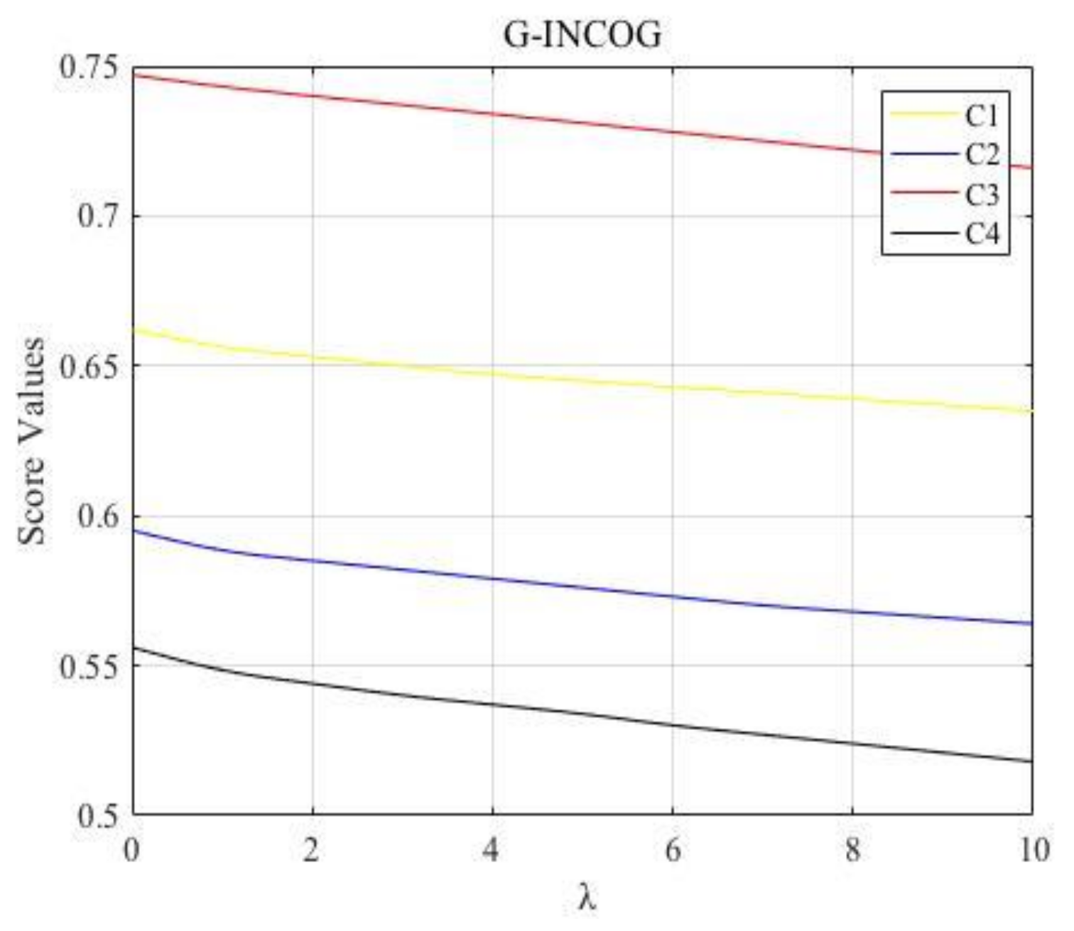
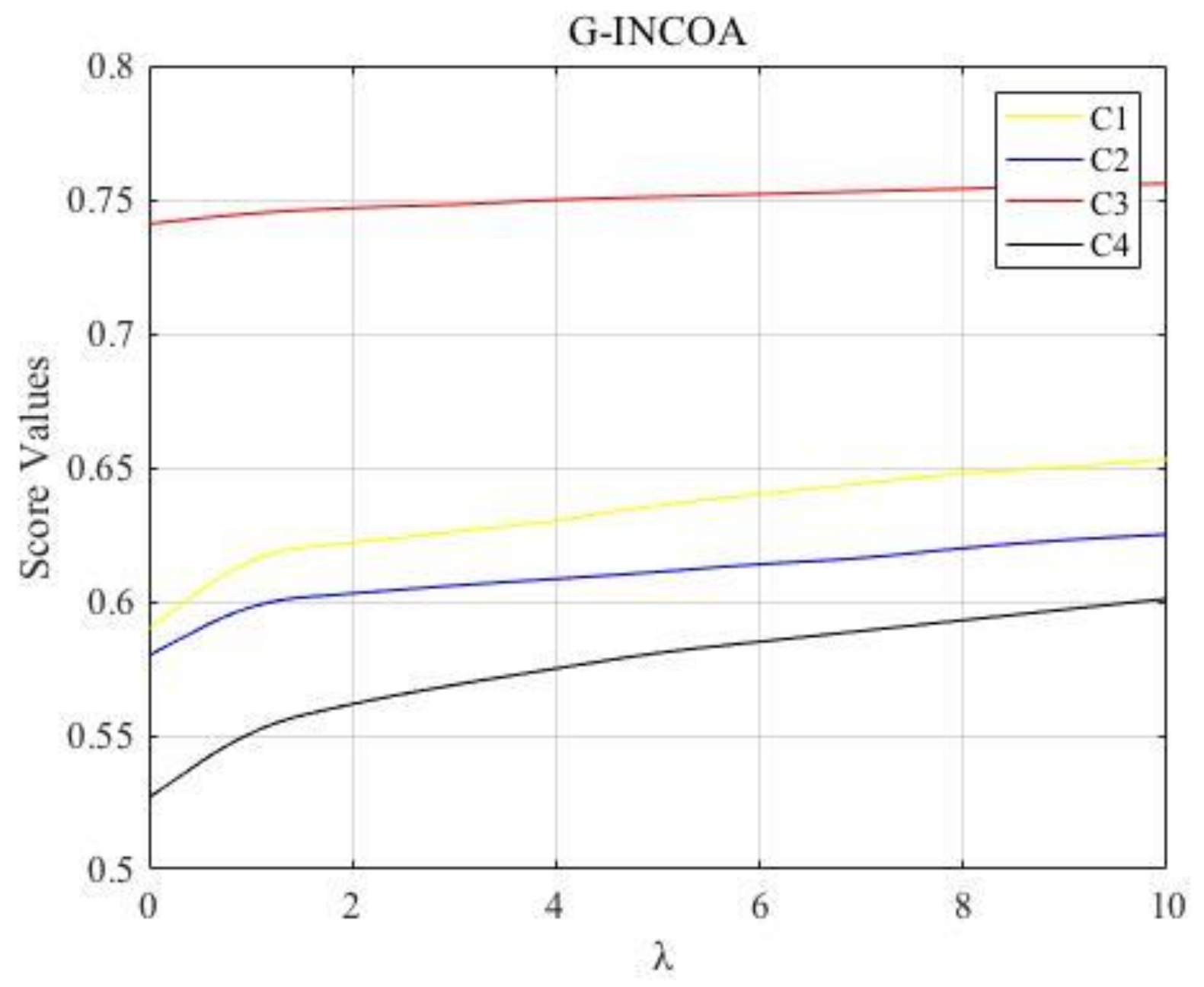
4.3. Rank Alternatives for Different Values of $\lambda$

In real life, decision makers may determine the value of $\lambda$ by different MADM problems or their preferences, which makes the decision-making process more flexible. In this section, we use different values of parameter $\lambda$ of the G-INCOA and G-INCOG operators, such as $\lambda \to 0\mathrm{or}\lambda =1-10,$ to rank alternatives of the numerical example in Section 4.2.

Combined with the proposed approaches for MADM with interval neutrosophic information, we can obtain their score function values of four alternatives, the ranking results for different values of $\lambda$ determined by the G-INCOA and G-INCOG operator are shown in Figure 1 and Figure 2, respectively. As shown in Figure 1 and Figure 2, the best choice is always $a_3$ and the worst alternative is always $a_4$, which means they have higher accuracy and greater reference value. Besides, the changing trends of decision results with parameter $\lambda$ calculated by the G-INCOA operator presents an increasing trend, meanwhile, the changing trends of decision results with $\lambda$ calculated by the G-INCOG operator shows a declining trend, which further validates the duality of the proposed operators.

5. Apply the Proposed Operators for INSs to Cluster Analysis

5.1. New Clustering Algorithm for INSs

In this section, we intend to propose a new clustering algorithm for INSs to illustrate the efficiency of the proposed operators. Let $N={({\tilde{n}}_{ij}=\{{\tilde{t}}_{ij},{\tilde{i}}_{ij},{\tilde{f}}_{ij}\})}_{n\times m}$ be a matrix of INNs on $X=\{X_1,X_2,\dots ,X_m\}$, the algorithm can be described as:

Step 1. Using the proposed operator, here, take the G-INCOA operator as an example, to aggregate m INNs of each alternative to an comprehensive INN ${\tilde{n}}_i$; Using the similarity measures function defined in Equation (3) to calculate measures between ${\tilde{n}}_j$ and ${\tilde{n}}_k\left(j,k=1,2,\dots ,m\right)$, the corresponding results are recorded in a matrix $S_{m\times m}=S_{jk}$;

Step 2. Check whether the measure matrix S satisfies $S^2\subseteq S,$ where $S^2=S\circ S={\left(S_{jk}^{\prime }\right)}_{m\times m},$ and ${\tilde{n}}_{jk}^{\prime }=ma{x}_p\left\{min\left\{S_{jp},S_{pk}\right\}\right\},\left(j,k=1,2,\dots ,m\right).$ If it does not hold, then construct the equivalent matrix: $S^{2^p}:S\to S^2\to S^4\to \dots \to$ until $S^{2^p}=S^{2^{\left(p+1\right)}}$;

Step 3. For a given confident level $\alpha \in [0,1],$ construct a $\alpha$-cutting matrix $S_{\alpha }={\left(S_{jk}^{\alpha }\right)}_{m\times m}$, where $S_{jk}^{\alpha }$ is defined as:

$$S_{jk}^{\alpha }=\{\begin{array}{c}0,\mathrm{if}{S}_{jk}<\alpha ;\\ 1,\mathrm{if}{S}_{jk}\ge \alpha .\end{array}$$

Step 4. Classify the INSs by the rule: if all elements of the jth line in $S_{\alpha }$ are the same as the corresponding elements of the kth line, thus, the INSs ${\tilde{n}}_j$ and ${\tilde{n}}_k$ are supposed as the same type.

5.2. Numerical Example

A numerical example concerning investing is utilized to demonstrate the application of these aggregation operators, as well as the effectiveness of them. Suppose there are five attributes to be considered: (1) $X_1:$ profitability; (2) $X_2:$ operating capacity; (3) $X_3:$ market competition. The fuzzy measures of attributes in X are given as follows: $\mu \left(x_1\right)=0.362,\mu \left(x_2\right)=0.2,\mu \left(x_3\right)=0.438$. Firstly, according to Equation (7), the value of ${\mathsf{\lambda }}_g$ is obtained: ${\mathsf{\lambda }}_g=0.856$. Thus,$\mu \left(x_1,x_2\right)=0.626,\mu \left(x_2,x_3\right)=0.713,\mu \left(x_1,x_3\right)=0.936,\mu \left(X\right)=1$. Experts are required to evaluate 10 firms $C_i\left(i=1,2,\dots ,10\right)$ under the three attributes, and interval neutrosophic decision matrix $N={\left({\tilde{n}}_{ij}\right)}_{10\times 3}$ is constructed as:

$$N=\left(\begin{array}{ccc}\left([0.3,0.5],[0.5,0.6],[0.4,0.6]\right)& \left([0.4,0.5],[0.4,0.6],[0.4,0.5]\right)& \left([0.7,0.8],[0.2,0.3],[0.3,0.5]\right)\\ \left([0.4,0.6],[0.3,0.5],[0.3,0.7]\right)& \left([0.6,0.8],[0.3,0.4],[0.2,0.4]\right)& \left([0.2,0.3],[0.8,0.9],[0.7,0.8]\right)\\ \left([0.5,0.7],[0.2,0.3],[0.4,0.5]\right)& \left([0.7,0.9],[0.2,0.4],[0.1,0.2]\right)& \left([0.3,0.4],[0.5,0.7],[0.7,0.8]\right)\\ \left([0.3,0.5],[0.4,0.6],[0.5,0.8]\right)& \left([0.8,0.9],[0.1,0.2],[0.2,0.3]\right)& \left([0.7,0.9],[0.2,0.3],[0.2,0.3]\right)\\ \left([0.8,1.0],[0.2,0.3],[0.1,0.3]\right)& \left([0.8,1.0],[0.1,0.2],[0.1,0.3]\right)& \left([0.4,0.6],[0.3,0.4],[0.4,0.6]\right)\\ \left([0.4,0.6],[0.4,0.6],[0.5,0.7]\right)& \left([0.2,0.3],[0.6,0.8],[0.7,0.9]\right)& \left([0.9,1.0],[0.1,0.2],[0.1,0.2]\right)\\ \left([0.5,0.6],[0.4,0.5],[0.5,0.6]\right)& \left([0.7,0.9],[0.2,0.3],[0.2,0.4]\right)& \left([0.6,0.8],[0.3,0.4],[0.2,0.5]\right)\\ \left([0.9,1.0],[0.1,0.2],[0.1,0.2]\right)& \left([0.7,0.8],[0.2,0.3],[0.3,0.4]\right)& \left([0.4,0.5],[0.4,0.6],[0.5,0.7]\right)\\ \left([0.4,0.6],[0.6,0.7],[0.2,0.4]\right)& \left([0.9,1.0],[0.1,0.2],[0.1,0.2]\right)& \left([0.6,0.7],[0.3,0.4],[0.3,0.5]\right)\\ \left([0.8,0.9],[0.2,0.4],[0.2,0.3]\right)& \left([0.6,0.8],[0.3,0.5],[0.3,0.4]\right)& \left([0.5,0.8],[0.3,0.6],[0.4,0.5]\right)\end{array}\right).$$

In the following, we use the proposed clustering algorithm to cluster these alternatives:

Step 1. Aggregated the G-INCOA operator defined in Equation (8) and calculated by the similarity measure function defined in Equation (5), the weighted measures $S_{jk}$ between each pair of alternatives are recorded in a matrix $S_{10\times 10}$.

$$S=\left(\begin{array}{cccccccccc}1& 0.5984& 0.458& 0.4635& 0.3964& 0.7100& 0.5572& 0.4761& 0.4143& 0.3984\\ 0.5984& 1& 0.5& 0.5136& 0.4456& 0.4667& 0.5409& 0.5456& 0.5051& 0.3851\\ 0.4580& 0.5& 1& 0.6811& 0.5596& 0.4080& 0.6994& 0.6875& 0.6682& 0.4753\\ 0.4635& 0.5136& 0.6811& 1& 0.5421& 0.4540& 0.7236& 0.6744& 0.731& 0.4747\\ 0.3964& 0.4456& 0.5596& 0.5421& 1& 0.3762& 0.5734& 0.6517& 0.625& 0.7511\\ 0.7100& 0.4667& 0.4080& 0.4540& 0.3762& 1& 0.5431& 0.4647& 0.3813& 0.4019\\ 0.5572& 0.5409& 0.6994& 0.7236& 0.5734& 0.5431& 1& 0.7023& 0.6726& 0.5211\\ 0.4761& 0.5456& 0.6875& 0.6744& 0.6517& 0.4647& 0.7023& 1& 0.6615& 0.6063\\ 0.4143& 0.5051& 0.6682& 0.7310& 0.6250& 0.3813& 0.6726& 0.6615& 1& 0.5372\\ 0.3984& 0.3851& 0.4753& 0.4747& 0.7511& 0.4019& 0.5211& 0.6063& 0.5372& 1\end{array}\right).$$

Step 2. The equivalent measure matrix can be constructed as follows, as $S^8=S^4$, therefore, $S^4$ is an equivalent measure matrix.

$$S^2=\left(\begin{array}{cccccccccc}1& 0.5984& 0.5572& 0.5572& 0.5572& 0.5431& 0.5572& 0.5572& 0.5572& 0.5211\\ 0.5984& 1& 0.5456& 0.5456& 0.5456& 0.5984& 0.5572& 0.5456& 0.5456& 0.5456\\ 0.5572& 0.5456& 1& 0.6994& 0.6517& 0.5431& 0.6994& 0.6994& 0.6811& 0.6063\\ 0.5572& 0.5456& 0.6944& 1& 0.6517& 0.5431& 0.7236& 0.7023& 0.7310& 0.6063\\ 0.5572& 0.5456& 0.6517& 0.6517& 1& 0.5431& 0.6517& 0.6517& 0.6517& 0.7511\\ 0.5431& 0.5984& 0.5431& 0.5431& 0.5431& 1& 0.5572& 0.5431& 0.5431& 0.5211\\ 0.5572& 0.5572& 0.6994& 0.7236& 0.6517& 0.5572& 1& 0.7023& 0.7236& 0.6063\\ 0.5572& 0.5456& 0.6994& 0.7023& 0.6517& 0.5431& 0.7023& 1& 0.6744& 0.6517\\ 0.5572& 0.5456& 0.6811& 0.7310& 0.6517& 0.5431& 0.7236& 0.6744& 1& 0.6520\\ 0.5211& 0.5456& 0.6063& 0.6063& 0.7511& 0.5211& 0.6063& 0.6517& 0.6250& 1\end{array}\right).$$

$$S^4=\left(\begin{array}{cccccccccc}1& 0.5984& 0.5572& 0.5572& 0.5572& 0.5984& 0.5572& 0.5572& 0.5572& 0.5572\\ 0.5984& 1& 0.5572& 0.5572& 0.5572& 0.5984& 0.5572& 0.5572& 0.5572& 0.5572\\ 0.5572& 0.5572& 1& 0.6994& 0.6517& 0.5431& 0.6994& 0.6994& 0.6944& 0.6517\\ 0.5572& 0.5572& 0.6944& 1& 0.6517& 0.5572& 0.7236& 0.7023& 0.7310& 0.6517\\ 0.5572& 0.5572& 0.6517& 0.6517& 1& 0.5572& 0.6517& 0.6517& 0.6517& 0.7511\\ 0.5984& 0.5984& 0.5572& 0.5572& 0.5572& 1& 0.5572& 0.5572& 0.5572& 0.5572\\ 0.5572& 0.5572& 0.6994& 0.7236& 0.6517& 0.5572& 1& 0.7023& 0.7236& 0.6517\\ 0.5572& 0.5572& 0.6994& 0.7023& 0.6517& 0.5572& 0.7023& 1& 0.7023& 0.6517\\ 0.5572& 0.5572& 0.6944& 0.7310& 0.6517& 0.5572& 0.7236& 0.7023& 1& 0.6520\\ 0.5572& 0.5572& 0.6517& 0.6517& 0.7511& 0.5572& 0.6517& 0.6517& 0.6517& 1\end{array}\right).$$

$$S^8=\left(\begin{array}{cccccccccc}1& 0.5984& 0.5572& 0.5572& 0.5572& 0.5984& 0.5572& 0.5572& 0.5572& 0.5572\\ 0.5984& 1& 0.5572& 0.5572& 0.5572& 0.5984& 0.5572& 0.5572& 0.5572& 0.5572\\ 0.5572& 0.5572& 1& 0.6994& 0.6517& 0.5431& 0.6994& 0.6994& 0.6944& 0.6517\\ 0.5572& 0.5572& 0.6944& 1& 0.6517& 0.5572& 0.7236& 0.7023& 0.7310& 0.6517\\ 0.5572& 0.5572& 0.6517& 0.6517& 1& 0.5572& 0.6517& 0.6517& 0.6517& 0.7511\\ 0.5984& 0.5984& 0.5572& 0.5572& 0.5572& 1& 0.5572& 0.5572& 0.5572& 0.5572\\ 0.5572& 0.5572& 0.6994& 0.7236& 0.6517& 0.5572& 1& 0.7023& 0.7236& 0.6517\\ 0.5572& 0.5572& 0.6994& 0.7023& 0.6517& 0.5572& 0.7023& 1& 0.7023& 0.6517\\ 0.5572& 0.5572& 0.6944& 0.7310& 0.6517& 0.5572& 0.7236& 0.7023& 1& 0.6520\\ 0.5572& 0.5572& 0.6517& 0.6517& 0.7511& 0.5572& 0.6517& 0.6517& 0.6517& 1\end{array}\right).$$

Step 3. For a given confident level $\alpha \in [0,1],$ we can construct a $\alpha$-cutting matrix $S_{\alpha }={\left(S_{jk}^{\alpha }\right)}_{10\times 10}$ for $S^8={\left(S_{jk}^{}\right)}_{10\times 10}$, different $\alpha$ produces different $\alpha$-cutting matrix, for example, if $\alpha =0,$ the $\alpha$-cutting matrix can be constructed as $S_{\alpha }={\left(S_{jk}^{\alpha }=1\right)}_{10\times 10}$, since $S^8={\left(S_{jk}^{}>0\right)}_{10\times 10}$.

Step 4. Based on the $\alpha$-cutting matrix $S_{\alpha },$ we can classify 10 alternatives into different clusters, the possible classification of these choices is shown in

Table 2. Different clusters of 10 alternatives with respect to different $\alpha$.

Class	Confidence Level	Clusters
8	$0.731<\alpha \le 1$	$\{\{C_1\},\{C_2\},\{C_3\},\{C_4\},\{C_5\},\{C_6\},\{C_7\},\{C_8\},\{C_9\},\{C_{10}\}\}$
7	$0.7236<\alpha \le 0.731$	$\{\{C_1\},\{C_2\},\{C_3\},\{C_4,C_9\},\{C_5\},\{C_6\},\{C_7\},\{C_8\},\{C_{10}\}\}$
6	$0.7023<\alpha \le 0.7236$	$\{\{C_1\},\{C_2\},\{C_3\},\{C_4,C_7,C_9\},\{C_5\},\{C_6\},\{C_8\},\{C_{10}\}\}$
5	$0.6994<\alpha \le 0.7023$	$\{\{C_1\},\{C_2\},\{C_3\},\{C_4,C_7,C_8,C_9\},\{C_5\},\{C_6\},\{C_{10}\}\}$
4	$0.6517<\alpha \le 0.6994$	$\{\{C_1\},\{C_2\},\{C_3,C_4,C_7,C_8,C_9\},\{C_5,C_{10}\},\{C_6\}\}$
3	$0.5984<\alpha \le 0.6517$	$\{\{C_1\},\{C_2\},\{C_3,C_4,C_5,C_7,C_8,C_9,C_{10}\},\{C_6\}\}$
2	$0.5572<\alpha \le 0.5984$	$\{\{C_1,C_2,C_6\},\{C_3,C_4,C_5,C_7,C_8,C_9,C_{10}\}\}$
1	$0<\alpha \le 0.5572$	$\{\{C_1,C_2,C_3,C_4,C_5,C_6,C_7,C_8,C_9,C_{10}\}\}$

.

With respect to different values of $\alpha$, different clusters of 10 alternatives are shown in Table 2. When $0<\alpha \le 0.5572,$ all alternatives belong to the same cluster, then $0.5572<\alpha \le 0.5984,$ 10 alternatives are divided in to two clusters, namely, $\{C_3,C_4,C_5,C_7,C_8,C_9,C_{10}\}$ and $\{C_1,C_2,C_6\},$ until $0.731<\alpha \le 1$, each alternative is an independent cluster.

6. Conclusions

This paper studies new MADM methods and clustering algorithm under an interval neutrosophic environment, in which the attributes are inter-related. Motivated by the idea of the generalized operator, we proposed the G-INCOA and G-INCOG operators based on the related research of the NS and SVNS theories, which can reduce to the existing aggregation operators of INSs and have some desirable properties. By taking different values of the parameters and comparing them with existing methods for MADM problems, under interval neutrosophic environment, results obtained by the proposed operators are consistent and accurate, which illustrates their practicability in application. The new clustering algorithm are established on the G-INCOA and G-INCOG operators, a numerical example concerning investing is utilized as the demonstration of the application of the proposed aggregation operators, as well as the effectiveness of them. In the future, motivated by different MADM methods under linguistic environment [34,35], it is worth investigating the use granular computing techniques to develop new MADM methods with interval neutrosophic linguistic information.

References

- Ye, J. Multicriteria decision-making method using the correlation coefficient under single-valued neutrosophic environment. Int. J. Gen. Syst. 2013, 42, 386–394. [Google Scholar] [CrossRef]
- Zadeh, L.A. Fuzzy sets. Inf. Control 1965, 8, 338–353. [Google Scholar] [CrossRef]
- Torra, V.; Narukawa, Y. On hesitant fuzzy sets and decision. In Proceedings of the 18th IEEE International Conference on Fuzzy Systems, Jeju Island, Korea, 20–24 August 2009; pp. 1378–1382. [Google Scholar] [CrossRef]
- Zhang, X.H. Fuzzy anti-grouped filters and fuzzy normal filters in pseudo-BCI algebras. J. Intell. Fuzzy Syst. 2017, 33, 1767–1774. [Google Scholar] [CrossRef]
- Smarandache, F. A Unifying Field in Logics: Neutrosophic Logic, Neutrosophy, Neutrosophic Set, Neutrosophic Probability; American Research Press: Rehoboth, DE, USA, 1999. [Google Scholar]
- Wang, H.; Madiraju, P. Interval-neutrosophic Sets. J. Mech. 2004, 1, 274–277. [Google Scholar]
- Wang, H.; Smarandache, F.; Sunderraman, R. Single-valued neutrosophic sets. Rev. Air Force Acad. 2013, 17, 10–13. [Google Scholar]
- Broumi, S.; Smarandache, F.; Dhar, M. Rough neutrosophic sets. Ital. J. Pure. Appl. Math. 2014, 32. [Google Scholar] [CrossRef]
- Peng, J.; Wang, J.; Wu, X. Multi-valued neutrosophic sets and power aggregation operators with their applications in multi-criteria group decision-making problems. Int. J. Comput. Int. Syst. 2015, 8, 345–363. [Google Scholar] [CrossRef]
- Guo, Y.H.; Ümit, B.; Şengür, A.; Smarandache, F. A Retinal Vessel Detection Approach Based on Shearlet Transform and Indeterminacy Filtering on Fundus Images. Symmetry 2017, 9, 235–244. [Google Scholar] [CrossRef]
- Chen, J.Q.; Ye, J.; Du, S.G. Scale Effect and Anisotropy Analyzed for Neutrosophic Numbers of Rock Joint Roughness Coefficient Based on Neutrosophic Statistics. Symmetry 2017, 9, 14–27. [Google Scholar] [CrossRef]
- Zhang, X.H.; Bo, C.X.; Smarandache, F.; Dai, J.H. New inclusion relation of neutrosophic sets with applications and related lattice structrue. Int. J. Mach. Learn. Cybern. 2018. accepted. [Google Scholar]
- Akbulut, Y.; Sengur, A.; Guo, Y.H.; Smarandache, F. A Novel Neutrosophic Weighted Extreme Learning Machine for Imbalanced Data Set. Symmetry 2017, 9, 142. [Google Scholar] [CrossRef]
- Xu, Z.S.; Gou, X.J. An overview of interval-valued intuitionistic fuzzy information aggregations and applications. Granul. Comput. 2017, 2, 13–39. [Google Scholar] [CrossRef]
- Wang, C.Q.; Fu, X.G.; Meng, S.; He, Y. Multi-attribute decision making based on the SPIFGIA operators. Granul. Comput. 2017, 2, 321–331. [Google Scholar] [CrossRef]
- Jiang, Y.; Xu, Z.S.; Shu, Y.H. Interval-valued intuitionistic multiplicative aggregation in group decision making. Granul. Comput. 2017, 2, 387–407. [Google Scholar] [CrossRef]
- Joshi, B.P. Moderator intuitionistic fuzzy sets with applications in multi-criteria decision-making. Granul. Comput. 2018, 3, 61–73. [Google Scholar] [CrossRef]
- Chen, J.Q.; Ye, J.; Du, S.G. Vector Similarity Measures between Refined Simplified Neutrosophic Sets and Their Multiple Attribute Decision-Making Method. Symmetry 2017, 9, 153. [Google Scholar] [CrossRef]
- Hu, K.L.; Fan, E.; Ye, J.; Fan, C.; Shen, S.; Gu, Y. Neutrosophic Similarity Score Based Weighted Histogram for Robust Mean-Shift Tracking. Information 2017, 8, 122. [Google Scholar] [CrossRef]
- Zhang, H.Y.; Wang, J.Q.; Chen, X.H. Inverval neutrosophic sets and their application in multicriteria decision making problems. Sci. World J. 2014, 2014, 645953. [Google Scholar] [CrossRef]
- Broumi, S.; Smarandache, F. Correlation Coefficient of Interval Neutrosophic Set. Appl. Mech. Mater. 2013, 436, 511–517. [Google Scholar] [CrossRef]
- Zhang, H.Y.; Ji, P.; Wang, J.Q.; Chen, X.H. An Improved Weighted Correlation Coefficient Based on Integrated Weight for Interval Neutrosophic Sets and its Application in Multi-criteria Decision-making Problems. Int. J. Comput. Int. Syst. 2015, 8, 1027–1043. [Google Scholar] [CrossRef]
- Ye, J. Similarity measures between interval neutrosophic sets and their multicriteria decision-making method. J. Intell. Fuzzy Syst. 2014, 26, 165–172. [Google Scholar]
- Ye, J. Multiple attribute decision-making method based on the possibility degree ranking method and ordered weighted aggregation operators of interval neutrosophic numbers. J. Intell. Syst. 2015, 28, 1307–1317. [Google Scholar] [CrossRef]
- Liu, P.D.; Tang, G.L. Some power generalized aggregation operators based on the interval neutrosophic numbers and their application to decision making. J. Intell. Fuzzy. Syst. 2015, 30, 2517–2528. [Google Scholar] [CrossRef]
- Liu, P.D.; Teng, F. Multiple attribute decision making method based on normal neutrosophic generalized weighted power averaging operator. Int. J. Mach. Learn. Cybern. 2015, 1–13. [Google Scholar] [CrossRef]
- Liu, P.D.; Wang, Y.M. Interval neutrosophic prioritized OWA operator and its application to multiple attribute decision making. J. Syst. Sci. Complex. 2016, 29, 681–697. [Google Scholar] [CrossRef]
- Zhang, X.H.; She, Y.H. Fuzzy Quantifies with Integral Semantics; Science Press: Beijing, China, 2017; ISBN 978-7-03053-480-4. Available online: http://product.dangdang.com/25113577.html (accessed on 1 July 2017).
- Ju, Y.B.; Yang, S.H.; Liu, X.Y. Some new dual hesitant fuzzy aggregation operators based on Choquet integral and their applications to multiple attribute decision making. J. Intell. Fuzzy Syst. 2014, 27, 2857–2868. [Google Scholar] [CrossRef]
- Choquet, G. Theory of capacities. Ann. Inst. Fourier. 1953, 5, 131–295. [Google Scholar] [CrossRef]
- Sugeno, M. Theory of Fuzzy Integral and its Application. Ph.D. Thesis, Tokyo Institute of Technology, Tokyo, Japan, 22 January 1975. [Google Scholar]
- Liao, H.C.; Xu, Z.S.; Zeng, X.J. Novel correlation coefficients between hesitant fuzzy sets and their application in decision making. Knowl. Based Syst. 2015, 82, 115–127. [Google Scholar] [CrossRef]
- Chen, N.; Xu, Z.S.; Xia, M.M. Correlation coefficients of hesitant fuzzy sets and their applications to clustering analysis. Appl. Math. Model. 2013, 37, 2197–2211. [Google Scholar] [CrossRef]
- Liu, P.D.; You, X.L. Probabilistic linguistic TODIM approach for multiple attribute decision making. Granul. Comput. 2017, 2, 333–342. [Google Scholar] [CrossRef]
- Xu, Z.S.; Wang, H. Managing multi-granularity linguistic information in qualitative group decision making: An overview. Granul. Comput. 2016, 1, 21–35. [Google Scholar] [CrossRef]
Figure 1.
The changing trends of decision results with calculated by the G-INCOA operator.
Figure 2.
The changing trends of decision results with calculated by the G-INCOG operator.