A Hybrid MCDM Technique for Risk Management in Construction Projects
by
 , , ,
, , ,
Kajal Chatterjee
1,* ,
,
Edmundas Kazimieras Zavadskas
2 ,
,
Jolanta Tamošaitienė
2 ,
,
Krishnendu Adhikary
1 and
Samarjit Kar
1 1
Department of Mathematics, National Institute of Technology, Durgapur 713209, India
2
Faculty of Civil Engineering, Vilnius Gediminas Technical University, Sauletekio al. 11, LT-1022 Vilnius, Lithuania
*
Author to whom correspondence should be addressed.
Symmetry 2018, 10(2), 46; https://doi.org/10.3390/sym10020046
Submission received: 24 November 2017
/
Revised: 30 January 2018
/
Accepted: 9 February 2018
/
Published: 13 February 2018
(This article belongs to the Special Issue Civil Engineering and Symmetry)
Abstract
:Multi-stakeholder based construction projects are subject to potential risk factors due to dynamic business environment and stakeholders’ lack of knowledge. When solving project management tasks, it is necessary to quantify the main risk indicators of the projects. Managing these requires suitable risk mitigation strategies to evaluate and analyse their severity. The existence of information asymmetry also causes difficulties with achieving Pareto efficiency. Hence, to ensure balanced satisfaction of all participants, risk evaluation of these projects can be considered as an important part of the multi-criteria decision-making (MCDM) process. In real-life problems, evaluation of project risks is often uncertain and even incomplete, and the prevailing methodologies fail to handle such situations. To address the problem, this paper extends the analytical network process (ANP) methodology in the D numbers domain to handle three types of ambiguous information’s, viz. complete, uncertain, and incomplete, and assesses the weight of risk criteria. The D numbers based approach overcomes the deficiencies of the exclusiveness hypothesis and completeness constraint of Dempster–Shafer (D–S) theory. Here, preference ratings of the decision matrix for each decision-maker are determined using a D numbers extended consistent fuzzy preference relation (D-CFPR). An extended multi-attributive border approximation area comparison (MABAC) method in D numbers is then developed to rank and select the best alternative risk response strategy. Finally, an illustrative example from construction sector is presented to check the feasibility of the proposed approach. For checking the reliability of alternative ranking, a comparative analysis is performed with different MCDM approaches in D numbers domain. Based on different criteria weights, a sensitivity analysis of obtained ranking of the hybrid D-ANP-MABAC model is performed to verify the robustness of the proposed method.
1. Introduction
In recent decades, projects in the construction sector have become more complex and risky due to the diverse nature of activities among global companies [1,2,3,4,5,6,7,8]. In comparison to other sectors, construction projects encounter more risks due to uncertainties occurring because of various construction practices, working conditions, mixed cultures and political conditions between host and home countries [9,10,11,12]. Thus, in this scenario, risk management can be considered a vital part of the decision-making process in construction projects. These projects may involve many stakeholders, in addition to uncertain socio-economic conditions at the project site, bringing big challenges to practitioners of the industry in recent decades [13,14]. Construction project failure may cause higher costs and time over-runs, requiring a systematic risk assessment and evaluation procedure to classify and respond to changes [15,16].
Thus, prioritisation among construction based risk portfolios, and finding suitable risk mitigation strategies for construction projects, can be introduced as multi-criteria decision making (MCDM) problems. Researchers have recently proposed new methods for prioritising risks in construction based projects [10,17,18,19]. In addition, the increasing dynamism of construction projects has resulted in extensive impreciseness and subjectivities in this risk investigation procedure. With respect to the identification of risk criteria, a methodology is needed to sort and prioritise criteria weights, based on specific environments and domain experts’ judgment. In the real world, since various uncertainties occur in the decision-making process due to subjective and qualitative judgment of decision-makers (DMs), so it is essential to develop a more optimised technique that can handle various types of uncertainties [15,20,21,22,23,24].
In this scenario, a proper decision-making methodology is required to solve multiple conflicting interdependent criteria when evaluating risks in construction projects. In recent years, the number of papers related to analytic hierarchy process (AHP) and analytic network process (ANP) methods, considering supplier selection procedure, has increased substantially [25,26,27,28,29]. However, increasing the number of criteria or comparison levels causes confusion in decision makers’ (DMs) judgments, resulting in incomplete decision-making and inconsistency in the evaluator’s judgments, thus reducing strategy selection ability. Under these circumstances, Herrera-Viedma et al. [30] proposed consistent fuzzy preference relations (CFPR) to evade inconsistency in the decision-making process, and thus models have been developed with CFPR structuring of the problem of multi-criteria knowledge based strategy selection both with AHP [31] and ANP [32,33]. The CFPR methodology requires less time, has computational simplicity, and also guarantees consistency of decision matrices. However, as CFPR is based on complete and certain information, there always exists a possible inconsistency risk due to the inability of DMs to deal with overcomplicated objects [34].
It is obvious that the approaches mentioned above can play a vital role under some special circumstances, but it also reveals more uncertainties due to the subjective judgment of experts’ assessment. For fuzzy set theory it is difficult to determine in advance membership function values before making any decision in an uncertain and vague environment [8]. Interval theory has the same deficiency [23]. In addition, the frame of discernment and basic probability assignment (BPS) present in dempster–shafer (D–S) evidence theory limits its ability to represent incomplete information in uncertain situations [34,35]. In order to overcome the above shortcomings and effectively handle various uncertain and incomplete information, D numbers [36], a special kind of random set, is applied in the construction of CFPR. The D-CFPR [34] method expresses the expert’s linguistic preference values using D numbers, and can also be converted to traditional CFPR. In recent years, papers related to D numbers based MCDM methods have begun to appear, viz. D numbers based vlse kriterijumska optimizacija i kompromisno resenje (D-VIKOR) [37], D number based grey relational projection (D-GRP) [38], D numbers based analytic hierarchy process (D-AHP) [39,40], D numbers based technique for order of preference by similarity to ideal solution (D-TOPSIS) [41], and D numbers based decision-making trial and evaluation laboratory (D-DEMATEL) [42].
Besides managing the various risks associated with construction projects, this study also attempts to categorise and assess their risk mitigation strategies, thus setting up a proper framework that is accountable to investors in the construction sector. Thus, a survey on risk mitigation strategies is performed, based on the recent works [9,23,43], to alleviate construction projects risks. Based on the above considerations, this paper also develops an extended version of the MABAC methodology in an uncertain and incomplete decision environment, in order to evaluate risk mitigation strategies in construction based projects. Some papers related to MABAC have been published in recent years, viz. traditional DEMATEL-MABAC [44], pythagorean fuzzy MABAC [45], interval type 2 fuzzy MABAC [46], interval-valued intuitionistic fuzzy MABAC [47], and the fuzzy AHP-MABAC model [48].
Thus, the key motivation of this paper is to develop a D numbers based ANP-MABAC decision-making methodology for prioritising construction project risks, and to find suitable mitigating strategies in uncertain and incomplete decision environments. In this paper, we choose the ANP methodology due to its ability to represent the potential interactions, interdependences, and feedback among the risk based criteria and sub-criteria. Hesamamiri et al. [33] developed a systematic framework combining ANP and CFPR to properly assess and select a knowledge management strategy.
In this paper, CFPR is taken into the decision matrix under D-ANP to find the priority vectors of the criteria for uncertain and incomplete environments. Thus, the main objectives of this research are as follows:
- Categorise and describe proper risk issues concerning various socio-economic, technical, and geo-political based sectors correlated to construction projects.
- Develop a logical structure incorporating a D-CFPR based ANP model for risk prioritisation during construction.
- Identify and prioritise risk response factors in the construction industry based on the D-MABAC methodology.
This paper is organised as follows: Section 2 offers an outline of construction projects along with a review of risk assessment in the sector. Section 3 briefly discusses the preliminaries of D–S evidence theory and D numbers theory, along with their properties. In Section 4, algorithmic methodologies of D-CFPR, D-ANP, and D-MABAC are discussed. Section 5 demonstrates the effectiveness of the above methodology by presenting a numerical example on risk prioritisation and responses in the construction sector. A discussion based on sensitivity analysis is given in Section 6. Finally, the conclusions and future direction of the present research are given in Section 7.
2. Risks in Construction Projects
2.1. An Overview
The construction industry in general, as well as individual construction projects, deals with various threats, which are called risks. Risk assessment in construction projects has been applied differently from project to project (using various models of risk assessment) to evaluate the risk in certain activities of the project [49]. However, the socio-economic complexity involved in construction events makes it more risk prone, so that there may be negative effects on project sustainability [23]. Due to various complex factors, the construction industry is highly diverse and heterogeneous, experiencing a great deal of dynamic change with global sourcing and increasing price competition [50].
To overcome these risks, contractors have generally used high mark-ups, but this approach is no longer effective, as their margins have become smaller [51]. In recent decades, the stages involved in construction projects have become far more complex in nature, due to technological upgrading and stakeholder pressure, and are characterised by a number of uncertainties, which have a negative influence on the projects [52]. As risk free construction projects are impossible in real life, a controlled risk assessment procedure is required to manage various risks in the projects. The aim of this study is to highlight the main risks that construction projects face and the risk mitigation strategies used to manage them.
2.2. Previous Studies on Risk Assessment in Construction Projects
There have been substantial developments over the last four decades in research related to construction project management. Projects have been considered that are either exposed to risks, or have apparently inherited risk due to the participation of several stakeholders (as owners, contractors and designers); see [53] among others. For classifying and managing risks effectively, many methodologies have been suggested in the literature. In this section, a list of the existing approaches to construction project risk management is now briefly summarised.
Wang et al. [4] developed an alien eyes’ risk (AER) model, categorising the project risks and their mutual relationships, and proposing a qualitative risk mitigation framework. Schieg [17] adopted a risk management process in construction project management, concentrating more on personal area risks. Zavadskas et al. [23] presented risk assessment based on the MCDM method and applying TOPSIS grey and grey number based complex proportional assessment (COPRAS-G). Wen [54] integrated rough sets and artificial neural networks (ANN) for risk evaluation of construction projects. Fouladgar et al. [55] proposed a risk evaluation outline faced during tunneling operations based on fuzzy TOPSIS methodology. Taroun and Yang [56] hybridised the dempster–shafer (D–S) theory of evidence and evidential reasoning algorithm for structuring personal experience and professional judgment with a spreadsheet-based decision support system. Mohammadi and Tavakolan [25] combined fuzzy logic and AHP in traditional failure mode effect analysis (FMEA) for construction project risk assessment. Serpella et al. [18] applied a knowledge-based approach, based on a three-fold arrangement and risk management function, to address project risks in the construction management sector. Ebrat and Ghodsi [14] identified the risks in construction projects based on the adaptive neuro fuzzy inference system and stepwise regression model for the evaluation of project risks. Taylan et al. [15] proposed hybrid methodologies combining fuzzy AHP and fuzzy TOPSIS and applied the relative importance index method to prioritise the project risks based on the data obtained. Iqbal et al. [9] considered two types of risk management technique during project execution, viz. preventive techniques (to manage risk before the start of the project) and remedial techniques (after occurrence of the risk). Vafadarnikjoo et al. [24] developed an intuitive fuzzy decision-making trial and evaluation laboratory (DEMATEL) to prioritise risks associated with construction projects by using the risk breakdown structure. Ahmadi et al. [27] analysed the criteria for prioritising potential risk events and quantified it using fuzzy AHP. The best response action for a risk event is then identified with respect to the same criteria using a scope expected deviation index. Santos and Jungles [19] evaluate the completion of construction project risk by considering the correlation of delay and the schedule performance index along with any time over-run. Shin et al. [28] made a comparative analysis of AHP and fuzzy AHP to evaluate the potential risk factors at the construction site of a nuclear power plant. Kao et al. [57] proposed an integrated fuzzy ANP based balanced scorecard system for evaluation of relevant bilateral factors in Taiwanese construction projects. Burcar Dunovic et al. [58] assessed large infrastructure projects by integrating the risk impact cumulative distribution curve based MCDM approach. Yousefi et al. [59] proposed a neural network model for predicting emerging time and cost claims applied to Iranian construction projects. Valipour et al. [60] presented a fuzzy cybernetic ANP model for proper identification of public-private partnership project based risks. Ulubeyli and Kazaz [61] developed a fuzzy based sub-contractor selection model (CoSMo) for global based construction projects. Rajakallio et al. [62] analysed the solution delivery from a network perspective in integrated business model renewal. For assessing risk in deep foundation excavation, Valipour et al. [63] developed a step-wise weight assessment ratio analysis (SWARA) based complex proportional assessment (COPRAS) framework to analyse Iranian construction project uncertainty. Khanzadi et al. [64] solved the dispute resolution problem in the construction sector by considering a grey number based discrete zero-sum two-person matrix game model. Keshavarz Ghorabaee et al. [65] presented the hybrid fuzzy step-wise weight assessment ratio analysis (SWARA) based ‘evaluation based on distance from average solution’ (EDAS) model for assessment of the construction equipment by taking sustainability into account.
3. Preliminaries
3.1. Dempster–Shafer (D–S) Evidence Theory
To deal with real world information, which may be ambiguous, various imprecise decision-making models based on probability theory, fuzzy set theory, and D–S evidence theory have been developed [66]. D–S evidence theory directly expresses uncertain information by allocating the probability to the multiple object based subsets in lieu of individual items [67]. Due to its ability to compare pairs of evidence or belief functions when deriving new ones, and its superiority in an uncertain environment, evidence theory has been widely applied in various domains [22,34,39,68,69,70].
Certain basic definitions are now presented. Let denote the frame of discernment representing a collective set of exhaustive and mutually exclusive events, and each element of (a power set in ) represents a proposition [22]. Based on these, basic probability assignment (BPA) is defined as follows:
Definition 1.
Basic Probability Assignment (BPA)
A finite non-empty set of mutually exclusive and exhaustive hypotheses for any problem domain is called its frame of discernment. In lieu of a D–S evidence framework, the BPA is defined on a frame of discernment to express the imprecise judgements of experts [39]. Thus, if denotes the power set of a finite non-empty set , then a BPA is defined as a mapping m satisfying (1) and (2):
where is an empty set and is any element of . If is called its focal element, and the union of all focal elements is the core of the mass function.
Example: Suppose there exists a task to assess a project. In the frame of D–S theory, the frame of discernment is the proposed project set .
As per the expert view, a BPA can be created to express their assessment result: , where . In addition, the set is a frame of discernment in D–S theory with .
3.2. D Numbers Theory
Although D–S evidence theory is operative in the data fusion problem, it is restricted to handling semantic information where linguistic variables are not mutually exclusive [39,70]. Intuitively, if some hypotheses of D–S theory are removed reasonably, the ability to represent and handle uncertain information may greatly improve. Overall, in many practical scenarios, the experts fail to have complete information, and the assessment is done solely on the basis of partial information, resulting in an incomplete BPA. Based on this idea, Deng [36] proposed numbers theory, a generalisation of evidence theory, in order to characterise ambiguous data, as defined in (3) and (4) below:
Definition 2.
D Numbers [36]
Let Ω be a finite nonempty set, numbers is defined by a mapping:
where is an empty set and is a subset of Ω.
- Firstly, D numbers with nonexclusive hypothesis in each element of the frame of discernment is more applicable for linguistic assessment.
- Secondly, in an evidence theory, a normal BPA must be complete, implying that the sum of all focal length elements in BPA is 1. D numbers allows the experts to input incomplete and uncertain information to the framework resulting in an incomplete BPA, thus releasing the completeness constraint. Thus, if the information is said to be complete, and for the information is said to be incomplete.
Example 1.
Let an expert give his assessment on the condition of a bridge, using D numbers, in a scale interval of [0,100]. The expert express his assessment in an incomplete BPA framework as follows:
where .
Hence, the set of is not a frame of discernment, because the elements in the above set are not mutually exclusive. In addition, since , the above information is incomplete. This example shows that the definition of D numbers is similar to the definition of the mass function.
Definition 3.
D numbers for a discrete set [36]
For a discrete set , where and , a special form of D numbers can be expressed as:
Two D numbers are said to be invariable if:
Example 2.
If there are two D numbers:
, then, .
Let be a D number; then, the integration representation of the D number is defined as:
Example 3.
Let , then .
4. Methodology
4.1. D-CFPR: D Numbers Extended CFPR
Based on the additive transitive property, Herrera-Viedma et al. [30] put forward the consistent fuzzy preference relation (CFPR) for structuring an decision matrix, which requires only pair wise comparisons, in lieu of comparisons needed for constructing a fuzzy preference relation. Preserving both the reciprocity and transitivity properties, CFPR is constructed only on complete and certain information but fails to deal with cases containing insufficient information [34,36]. Citing the same deficiency as in the case of fuzzy preference relations, Deng et al. [39] proposed the concept of a numbers preference relation encompassing the fuzzy preference relations of the numbers domain. In addition, considering the insufficiency in traditional CFPRs, Zuo et al. [42] proposed a D numbers consistent fuzzy preference relation matrix, abbreviated as D-CFPR matrix using D numbers to express linguistic preferences given by experts to construct the CFPR. In the following steps, we will discuss the algorithmic methodology of D-CFPR, where distribution assessments are assessed under incomplete or missing information.
Step 1: Construct a D-CFPR matrix . The D numbers extended CFPR is advocated to reinforce the capability of CFPR to express uncertain and incomplete information. A D numbers based preference relation on a set of criteria is characterized by a matrix on the product set , whose elements are formulated as per Equation (8), and represented in matrix form (9):
where , , . Obviously,
In Equation (9), is called a D-CFPR as it is constructed based on pair wise comparisons, denoted as representing a set of D numbers. Considering the set of preference values , the elements of which are denoted , which can also be represented as follows [42]:
where each component is obtained by:
where , is the component of is the component of is the component of
Thus, based on the reciprocal property, the rest of the entries in D-CFPR (9) are calculated as per Equation (11) as follows:
As per Equations (9)–(11), a D-CFPR can be constructed based on () pair wise comparisons . In the D-CFPR generated above, some values of the in that fall in the interval need to be transformed using Equation (12):
The transformation function (12) works as a normalisation, which transforms the values of from to the interval [0,1].
Step 2: Determine the crisp matrix. Convert the matrix in (9) to a crisp matrix (13) using the integration representation of D numbers (as per Equation (7)), where each element :
Step 3: Construct a probability matrix . Based on the crisp matrix (13), construct a probability matrix (14), representing the preference probability between a pair wise set of n criteria :
In the element where represents “prefer to”. Based on (13), a set of rules is suggested to generate .
- For the elements satisfying
- ○
- If then
- ○
- If then .
- When
- ○
- If then
- ○
- If then .
- when
In this condition, the unallocated preference (up) is . The probability of one criteria outperforming another criteria is as follows:
- ○
- If ,
- ○
- If then .
Step 4: Construct a triangular probability matrix . Rank the criteria using the triangularisation procedure, viz. by maximising the sum of the values above, the main diagonal in the square matrix in the final order is given as:
- First, sum up each row of the matrix and determine the row number with maximum value.
- Then, assuming the obtained row number is k, delete the k-th row and k-th column in the matrix.
- Replicate the two procedures above until the matrix is empty.
Thus, by applying this defined row deletion order operation on the matrix (14), construct the triangular probability matrix , shown in (15):
Step 5: Construct triangulated crisp matrix . Firstly, the crisp matrix (13) is triangulated based on the triangular matrix (15). From that step, the triangulated crisp matrix (16) is derived:
Secondly, for elements satisfying a new “polishing operation” (17) is implemented to obtain a triangulated crisp matrix (18):
Step 6: Calculate the relative priority weights of the criteria. Assume that the weight vector is , where are the weights of criteria . The elements above and alongside the main diagonal of the matrix (18) indicate the weight relationship of the criteria. Thus, by adding some necessary constraints, a set of Equation (19) is formed:
where indicates the granular information about the pairwise comparison, which reveals the expert’s perceptive competency. The value of each weight , subjected to the parameter , relates to the expert’s cognitive aptitude. The values of highly depend on the influence of the experts’ judgment and belief function. Thus, a feasible outline (20) is obtained as follows:
where signifies the lower bound of , , and n is the number of alternatives [39]. The concrete priority weight value of each criteria is calculated here when .
Step 7: Inconsistency for the D-CFPR. The traditional CFPR is fully consistent when constructed under the transitivity property for preference values. The D numbers based CFPR is consistent, but, when reduced to classical CFPR, it shows inconsistency under uncertain or incomplete information. Thus, to express this inconsistency of D-CFPRs, an inconsistency degree (ID) (21) is defined, based on the triangular probability matrix (18), as follows:
where is an element of and is the number of comparison objects. This emphasises that the inconsistency of the D matrix, and its acceptable level is decided by the DMs, whose subjective requirement regulates the tolerance level of the aforementioned inconsistency.
4.2. Evaluating the Risk Criteria Weight Using D-ANP
The evaluation of D-ANP methodology is composed of two phases.
The first phase emphasises the formation of pairwise judgments for every dependent relationship among given criteria , and determination of their priority weight. The priority weights thus obtained are input to the system-with-feedback supermatrix for computing the network influences amongst the different relationships.
The second phase, namely supermatrix evaluation, incorporates five steps: formation of the unweighted supermatrix, formation of the weighted supermatrix, normalisation of the weighted supermatrix (a column stochastic matrix), and finally convergence to a solution using the limited supermatrix.
The converged supermatrix will provide us with the relative priorities for each of the criteria (or sub-criteria) considered within clusters of the decision framework. Thus, the following algorithmic steps of D-ANP are as follows:
Step 1: Model construction and problem structuring. First, we properly outline the decision problem with detailed criteria and sub-criteria (if taken) and then delimit the cluster’s (dimension’s) network and elements (criteria set) within the given clusters. Next, we decide which inter- and inner-dependencies will prevail in the decision problem and clusters of the over-all feedback system.
Step 2: Pairwise comparison matrices and priority vectors. The expert inputs prerequisite for the ANP method are the pairwise judgments of the elements within each cluster, from which inter-and-inner-dependence matrices are formed. Primarily, three categories of pairwise comparisons are formed. First, the inner dependence comparison matrix, based on the criteria of different clusters (dimensions), is used to get the priority weight vector. Then, the pairwise comparison matrices obtained from criteria with respect to other factors (criteria) of the same cluster (dimension). Finally, the pairwise comparison matrix is developed by considering the factor (criteria) of a cluster (dimension) among factors (criteria) of the other cluster (dimension), which affect the criteria.
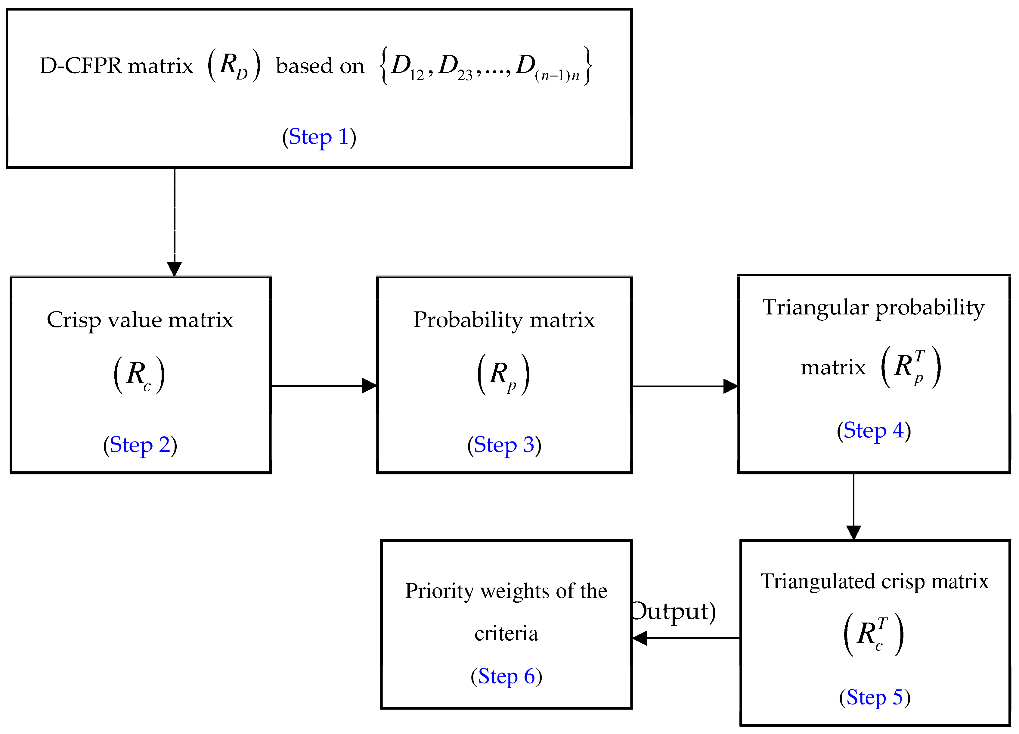
These pairwise comparison matrices, along with their valuation elicitation, constitute a modified version of D-AHP [22] and D-CFPR [34]. Based on Section 4.1, a brief summary for getting the priority weight of any pairwise comparison matrix is given below, the graphical description of which is shown in Figure 1.
- In the first step, the D-CFPR matrix , is constructed for n criteria, by considering the system as an input using Equations (9)–(12).
- The D-CFPR matrix formed , is converted to a crisp matrix , using the integration representation of D number, shown in Equation (13).
- The probability matrix is then constructed based on the derived crisp matrix using Equation (14), and it satisfies a set of rules in Step 3 of Section 4.1.
- In the next step, using Equation (15), triangularisation is applied to the probability matrix using local information that contains the preference relations of pairwise criteria.
- Lastly, applying Equations (16)–(19), the crisp based triangular matrix , is obtained, and relative priority weights of each criteria , based on clusters (dimensions) are calculated, thereby checking its inconsistency as per Equation (21).
Step 3: Formation of the unweighted supermatrix. The local priority weights resulting from the pairwise comparison are used as input in suitable columns of the unweighted constructed supermatrix, to obtain the global priorities in a system. As a result, a supermatrix takes the form of a partitioned matrix, each segment of which represents an association between two clusters in the given system. Thus, the supermatrix Equation (22) formed is represented by sub-matrices as . The size of the sub-matrix Equation (23) depends on the compared factors (criteria). Interdependency between clusters is illustrated in Equation (22) by analysing both inter- and intra-relations among clusters.
Arrange all priority vectors, representing the impact of a given set of elements in a cluster on another element in the network, as sub-columns of the corresponding column of an unweighted supermatrix as in Equations (22) and (23). This is composed of clusters , and linkages of these clusters , are elements of the cluster . Each column of the sub-matrix Equation (23) is the priority vector acquired from the identical pairwise judgment, indicating the significance of the elements in the cluster with respect to an element in the cluster:
Step 4: Determine the normalised weighted supermatrix. If there is no linkage between clusters and , then the sub-matrix equals zero. We compute the weighted supermatrix , by multiplying the unweighted matrix , Equation (23) by priority of dimensions , in this stage. As the weighted supermatrix needs to be stochastic, we normalise each column of it, and develop meaningful limiting priorities for determining overall cluster influences. This normalisation procedure ensures that the weighted supermatrix is column stochastic; it is finally represented by matrix .
Step 5: Compute the limiting priorities for criteria weights. Finally, the column stochastic weighted supermatrix is raised to an appropriately large power until it converges. Thus, the weighted supermatrix is raised to limiting powers , being an arbitrarily large number, to attain a steady-state limiting matrix . Details are shown in Equation (24):
The priority weight of criteria for the corresponding clusters (dimensions) can now be found in the rows of the limiting supermatrix . The limiting supermatrix provides the priority information for the elements of each individual cluster. The strategy outcome with the highest value should be selected from the cluster of criteria. Other priority rankings in different clusters are also provided.
4.3. D-MABAC for Ranking Alternatives
The MABAC methodology was developed by Pamucar and Cirovic [44] to handle problems in MCDM. D numbers is a new representation of uncertain information that can denote the more imprecise based conditions. Thus, the combination of MABAC and D numbers is a new experiment to make decisions in an uncertain environment. The basic setting of the MABAC technique is revealed in the definition of the distance of the criterion function of each of the observed alternatives from the approximate border area [72]. The algorithmic steps displays the execution process for the aforesaid D-MABAC methodology in six steps as follows:
Step 1: Constructing the initial decision matrix . Initially, the assessment of alternatives in respect of criteria is carried out. The alternatives are represented in vector form , where denotes the value (in D numbers format) for the alternative according to criteria for matrix . Details shown in decision-matrix (25):
Next, applying Equation (8), (i.e., integration representation of D numbers) on the elements of decision matrix , crisp decision matrix is formed as per Equation (26) as follows:
Step 2. Normalisation of the elements of the initial matrix . The elements of the normalized matrix are obtained using the following expressions:
where
where and the components , of the decision matrix represent the maximum and minimum values of the criteria , by alternatives .
Step 3. Calculation of the elements of weighted matrix . The elements of the weighted matrix , are calculated using the following equations:
where are the elements of the normalised matrix and the weight coefficients of criteria, respectively.
Step 4. Determine the border approximation area matrix (G). The elements of the border approximation area (BAA) for each criterion are determined as follows:
where are the elements of the weighted matrix , and is the total number of alternatives. After calculating the value , for each criterion, the BAA matrix is formed with format (n = the total number of criteria, according to which the selection is made from the alternatives).
Step 5. Calculation of the distance of the alternative from the BAA for the matrix elements . The distance of the alternatives from the BAA matrix is determined as the difference between the elements in the weighted matrix , and the value of the BAA . The distance are elements of a matrix and are shown in Equation (33):
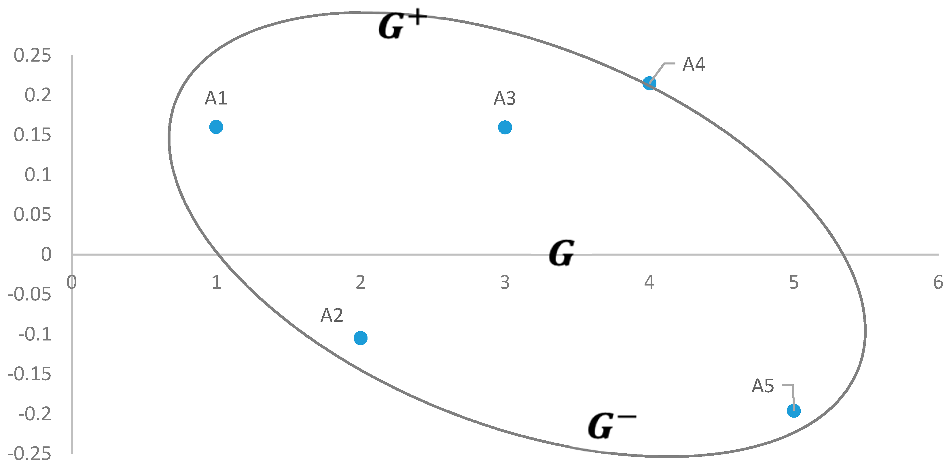
Alternative can belong to BAA , upper approximation area , or lower approximation area , and are determined as per Equation (34):
Step 6. Ranking of the alternatives. A calculation of the values of the criterion functions for the alternatives is obtained as the sum of the distance of the alternatives from the BAA . Using Equation (35), we calculate the sum of the elements of matrix by rows, and obtain the final values of the criterion functions , for the alternatives :
5. Numerical Example: Risk Assessment in a Construction Project
5.1. Identification of Construction Projects Risk Indicators and Their Mitigation Strategies
For categorising and managing construction project risks effectually, several methodologies are recommended in the literature [43,73,74,75]. Keeping this in mind, we proposed the hybrid D-ANP-MABAC approach for the risk assessment of projects in the construction sector involving uncertain and incomplete information data. The authors employed a combination of questionnaire surveys involving literature reviews and subjective judgments of highly proficient experts to detect different risk response strategies that optimise the performance of construction projects. The proposed methodology incorporates the knowledge and experience of ten experts (five technical and five management based experts) for risk identification and structuring, along with proper risk mitigation strategies. The demographic profile of the respondents is given in Table 1.
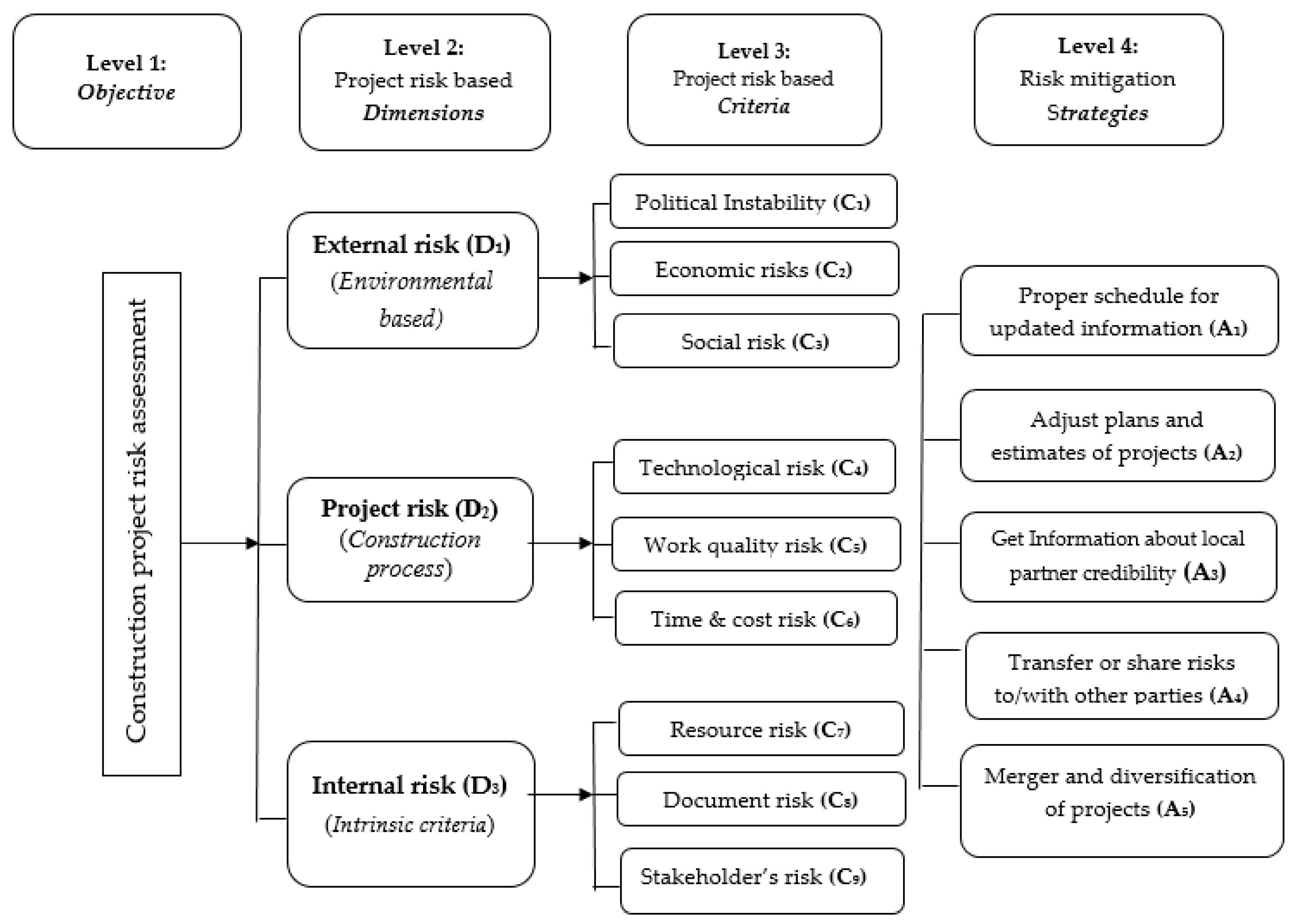
Based on the literature review of papers discussed in Table 2, the DMs consider nine construction project risk criteria identified under three dimensions: political instability (C1), economic risk (C2), and social risk (C3). These are defined as environmental based external risks (D1). Technological risk (C4), work quality risk (C5), and time and cost risk (C6) are defined as construction process based project risks (D2). Resource risk (C7), documents and information risk (C8), and stakeholder’s risk (C9) are defined under intrinsic criteria based internal risks (D3). Details are given below in Table 3.
In past decades, construction businesses were constrained to use only a limited number of risk management procedures, even though they were not suitable for all situations. For example, Lyons and Skitmore [50] found that brainstorming is the most common risk identification technique used in the Queensland engineering construction industry. Forbes et al. [74] developed a matrix for selecting appropriate risk management techniques such as artificial intelligence, probabilistic analysis, sensitivity analysis, and decision trees in the built environment for each stage of risk management. In this paper, based on the brainstorming method, the experts sought five alternative construction project risk response mitigation strategies, as detailed in Table 4.
5.2. Calculating Risk Based Criteria Weight Using D-ANP Framework
In this section, the weights of the risk based criteria in construction projects are calculated by D-ANP. The ANP has substantial influence in MCDM problems involving a wide range of factors and sub-factors. In the ANP, a decision problem is transformed into a network structure that allows both inter-intra dependency and feedback among the decision clusters, and even amongst elements within the same clusters. In this phase, the decision group is asked to make pairwise comparison matrices for priority weights of three dimensions and nine criteria (as detailed in Table 3).
Using Steps 1–6 (of Section 4.1) of D-CFPR, the priority weights are calculated in the decision matrices. The algorithmic steps of D-ANP are shown below:
Step 1: Construction of the hierarchy of criteria and alternative risks strategies. The clearly defined risk based construction project model is decomposed into a logical system like a network. Based on the hierarchy of Figure 2, we have five risk mitigation strategies in Level 4 hierarchical position, three dimensions (external, project, and internal risk) in Level 2, and corresponding to each dimension, a total of nine criteria in Level 3.
Step 2: Determination of the pairwise comparison matrices and priority vectors within clusters. The D numbers based preference matrix is first constructed before calculating the weight of the indicators using the ANP supermatrix. Here, we present the process of determining the priority weight of criteria (C1, C2, and C3) for risk dimension external risk with respect to the criterion C6 under dimension Project risk.
First, we calculate the relative significance of sub-criteria (C1, C2, and C3) relative to sub-criterion C6, to construct the inner dependence matrix built on the numbers based preference relation . In this case, the preference modelled by a set of numbers (based on DM’s choice) involving both uncertain entry (i.e., and incomplete entry , respectively:
The standard CFPR cannot handle this case, but D-CFPR (Equations (9)–(12) in Section 3.1) is effective to fill up the rest of the matrix elements in as follows:
Then, the D numbers based CFPR matrix is converted to a crisp mode, , using Equation (13), and the integration representation of D numbers Equation (7), shown below:
Applying the preference rules proposed for D-CFPR (in Step 3 of Section 4.1) and using Equation (14), the probability matrix is constructed:
Following the process (as mentioned in Step 4 of Section 4.1) of the D-CFPR methodology, we obtain the triangular matrix . Using the triangularisation method, the ranking of the indicators is calculated and shown as: where the symbol “” indicates preference,
We next evaluate the relative weights of the risk criteria. First, based on the ranking of the risk criteria in the triangulated matrix , the crisp matrix , is converted to a triangular crisp matrix , as per Equation (16):
Next, for elements satisfying a new polishing operation Equation (17) is executed and, by also applying Equation (18), a novel triangulated crisp matrix is obtained:
Finally, applying Equation (19), a group of equations is built to calculate the priority weight of each risk-based criterion. Applying the weight relation of the indicators in matrix mode, and incorporating necessary constraints, the weight equations are constructed and shown below:
where denotes the weight of the indicator and indicates the granular information about the pairwise evaluation, which is connected to the cognitive aptitude of the experts. Setting and using Equation (20), the weight of risk criteria C1, C2, and C3 for dimension D1 relative to C6 of dimension D2 are calculated as , respectively.
For quantifying the consistency of the D-CFPR based matrix , an ID defined for the D numbers preference relation (as defined in Equation (21)) is used to express such inconsistency, and, for the case study taken, it is found to be consistent.
Similarly, using the same process, the priority weights of remaining criteria, shown in Figure 3 with respect to the same dimensions and criteria of other clusters (dimensions), are calculated.
Step 3: Formation of unweighted supermatrix. Arrange all priority vectors, indicating the influence of pre-set elements, in different cluster elements in the network, as sub-columns of the resultant column in an unweighted supermatrix , which is composed of clusters , with corresponding linkages (criteria) . Putting , we get the first cluster (dimension) along with three elements representing three risk criteria , respectively. For , we get a second cluster (dimension) along with three elements representing three risk criteria . Similarly, the remaining cluster (dimensions) , along with its risk criteria, can be found. Thus, we get three clusters (dimensions) and nine corresponding risk criteria . Based on the above, the unweighted supermatrix is formed by placing priority vector elements in the particular column of , where each criterion influences the other risk criteria. Details shown in Table 5.
Step 4: Calculating the weighted supermatrix. The weighted supermatrix is calculated by multiplying unweighted supermatrix (Table 5) by the inner dependence matrix of risk dimension (Table 6). Details are shown in Table 7.
Step 5: Selecting the weight of criteria based on the limit matrix. To make the matrix column stochastic in Table 7, we normalise the weighted supermatrix column wise, and the result is shown in Table 8. The normalized weighted supermatrix (Table 8) is raised to its limiting power using Equation (22), to get the limiting supermatrix (Table 9). The final ranking of risk criteria weight for the construction project is shown in Table 10.
From Table 10, it is concluded that the third cluster (dimension) internal risk (D3) has a severe risk effect on the construction project sector. Document and information risk (C8) is the most risky, followed by resource risk (C7) and stakeholder’s risk (C9). First cluster External risk (D1) has less of a risk effect on construction business. Economic risk (C2) and social risk (C3) are in the 8th and 9th positions, respectively. However, political instability attains the 4th position in respect to the risk category. Managers and stakeholders should keep this in view when choosing projects in large construction sectors.
5.3. Determination of Final Alternative Ranking by D-MABAC
In this phase, the evaluation and ranking of risk response alternatives is performed by the application of a D numbers based MABAC (D-MABAC) methodology in construction project risk management. The step-by-step computational procedure is shown below.
Step 1: First, the five risk response alternative vectors, with respect to nine risk criteria , are represented as using incomplete and uncertain numbers expressed in D numbers. Using Equations (23) and (24), we develop an initial decision matrix (Table 11) along with its crisp form .
Step 2: The elements of the crisp decision matrix are normalized using Equations (24) and (25) to form a normalized decision matrix , shown in Table 12.
Step 3: Using Equations (26) and (27), the elements of the weighted normalized decision matrix are calculated, and are shown in Table 13.
Step 4: Next, using Equations (28) and (29), we determine the BAA, for each criterion . This is followed by calculation of the distance for matrix elements for risk response alternatives from BAA using Equations (30) and (31).
Step 5: Finally, using Equation (32), we calculate the sum function to obtain the ranking of alternatives . A graphical representation of the process is shown in Figure 4. Ranking of alternative risk response alternatives (Table 14) is finalised according to values calculated by D-MABAC in descending order. In this paper, the first alternative risk response was selected and implemented.
6. Results and Discussion
In this section, a detailed comparative analysis of all alternative initiatives (with respect to criteria and dimensions) is conducted.
6.1. Comparison of Alternative Ranking Using Different MCDM Methods
The hybrid MCDM methods in D numbers environment namely, D numbers based multi-attributive border approximation area comparison (D-MABAC), and D numbers based technique for order of preference by similarity to ideal solution (D-TOPSIS), D numbers based complex proportional assessment (D-COPRAS), and D numbers based additive ratio assessment (D-ARAS), were applied to the construction project based case study data to obtain the weighted normalised decision-making matrix (Table 13). The priority order of the risk response alternatives is compared and presented in Table 15.
Ranking of the risk response alternatives according to the presented MCDM methods concluded that the optimal alternative risk response is A1 (Proper scheduling for getting updated project information), followed by A3 (Information about local partner’s credibility), A4 (Transfer risks with other parties), and A2 (Adjust plans for scope of work). The worst performing risk response alternative is A5 (Merger and diversification of projects).
Spearman’s rank correlation coefficient between ranks is applied for determining correlation of ranks obtained by various approaches. Here, this coefficient is applied to demonstrate the statistical importance of difference among the ranking obtained through pairwise correlation analysis of different MCDM methods. Based on the recommendation of Keshavarz Ghorabaee et al. [65], all values higher than 0.80 show considerably high correlation. As per Table 16, a strong correlation (1.000) among the MCDM approaches is shown, confirming the credibility of the proposed approach.
6.2. Sensitivity Analysis
Ranking of results in MCDM problems are subject to the distribution of weight coefficients of the criteria. Sometimes, modifying these criteria weight coefficients may change the ranking order of alternatives, generally analysed by sensitivity analysis during the decision-making process. The above weight coefficients are usually based on expert subjective perception, and thus the outcome of probable deviation of these weight values need to be properly assessed.
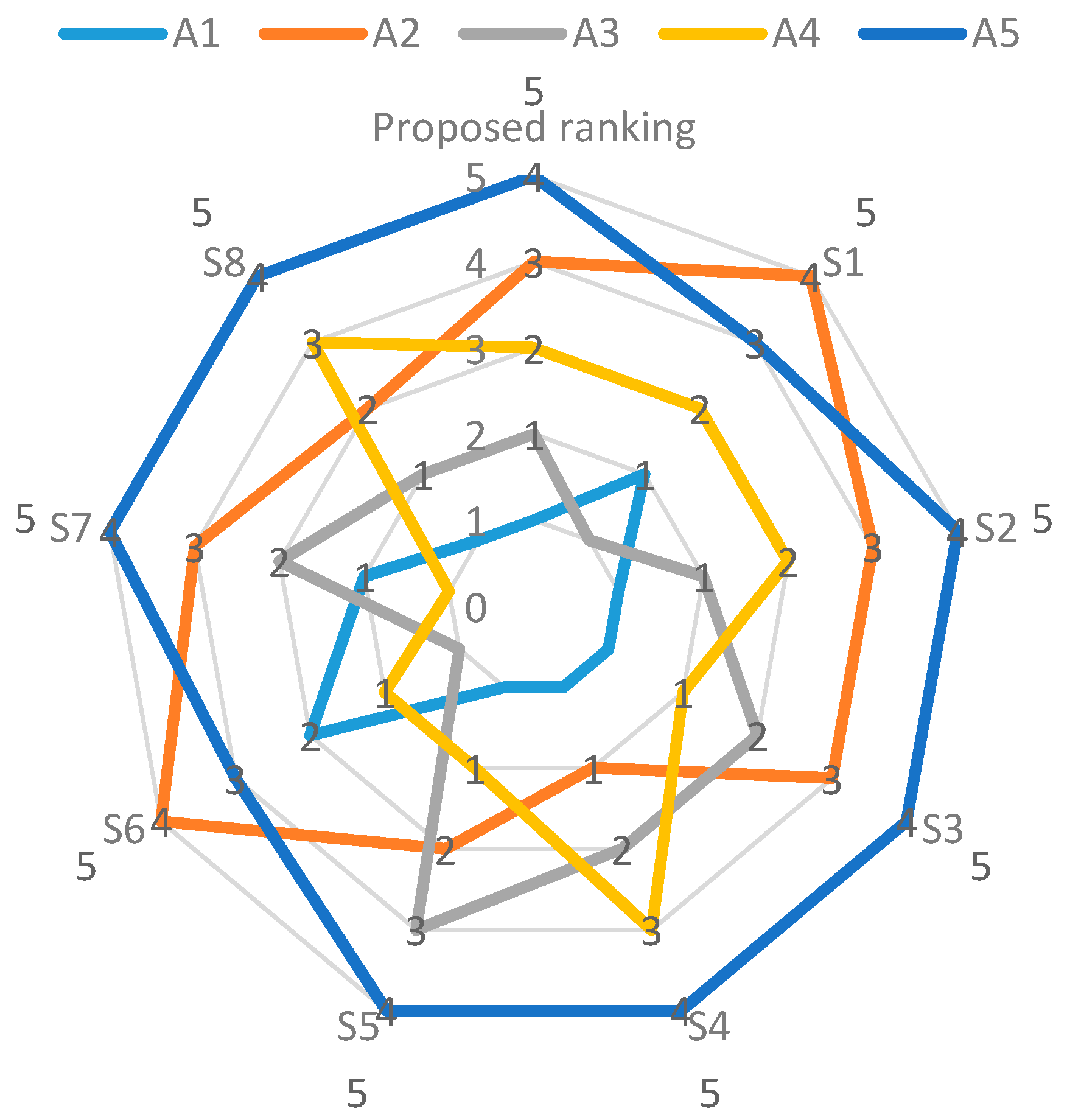
A sensitivity analysis was executed to measure the level of crosstalk amongst the criteria, revealing the variation in alternative rankings with variation in criteria weight. Outcomes of the sensitivity analysis for prioritising specific project based criteria weights are shown in Table 17, and its corresponding effect on ranking of risk response alternatives in Table 18.
- Analysis of the alternative ranking through eight scenarios (Table 18) showed that alternative A1 retained its rank in five scenarios (best-ranked alternative), while, in the remaining two scenarios , it was ranked second, and third in scenario .
- The worst-ranked alternative A5 retained its rank in six scenarios , while in two scenarios , it was ranked second worst. Therefore, changing the criteria weights through different scenarios resulted in changes to the ranks of the remaining alternatives.
- In addition, from Table 17 and Table 18, it is clear that prioritising criteria C9 has less of an effect on ranking position of alternatives. However, prioritising criteria set {C4, C6, and C7} in scenario S7, {C2, C6, and C8} in scenario S1, along with {C4, C6, and C8} in scenario S6, all altered the positions of risk response alternatives .
- The prioritising of criteria weight in scenarios has no effect on ranking of best or worst risk response alternative A1 and A5, respectively, but it does have an effect on the ranking of the second best risk response alternative A2.
7. Conclusions
Construction projects present a very complex field involving a large number of stakeholders. From the perspective of information sharing, uncertain information and data cause loss of faith among various stakeholders and increased risk in construction management, including project complexity and decision-making environment conditions. These risks affect project activities, which indirectly impact construction costs, resulting in delays and poor building quality. Thus, in this paper, we rank uncertain risk strategies in construction projects using a D-ANP-MABAC multi-criteria decision-making (MCDM) approach. In the new proposed method, the decision matrix determination from the MCDM problem is transformed to D numbers, which effectively represent the inevitable uncertainties such as incompleteness and imprecision, due to the subjective assessment of decision makers. As the basic element of many decision-making methods especially in analytic network process (ANP) model, the preference relation has attracted interests among researchers and practitioners. Fuzzy preference relation construct pairwise decision matrices based on linguistic values but is inconsistent due to inability of experts in dealing with overcomplicated objects. CFPR methodology [30] removes this inconsistency, but fails to deals with incomplete and uncertain information due to the lack of experts’ knowledge and the limitation of cognition. To overcome this weaknesses, D-CFPR methodology is applied to decision matrices allowing all stakeholders (members) of a construction business to address multiple criteria involving various types of uncertainties, such as imprecision and fuzziness in the decision process. The D-CFPR uses D numbers to express the linguistic preference values given by experts, and it can also be reduced to classical CFPR. Based on the D-CFPR based preference relation, the priority vectors of criteria are determined, to be used as inputs for any cluster of matrix formed by the D-ANP method, and obtain the corresponding risk criteria weights. The alternative risk response strategy ranking is achieved using the D-MABAC method.
In view of several categories of uncertainties, including incompleteness and impreciseness, the proposed technique can effectively represent and address uncertain information weighting risk criteria and alternatives in a logical way. An example of selecting risk strategies in construction risk projects is shown here to demonstrate the efficiency of the proposed approach. The assessment of a real world application of D-ANP-MABAC methodology, along with its output result of sensitivity, clearly identifies its potential to provide stable solutions to the problematic choice of laying-up positions. Based on that, the proposed risk strategy alternatives are successfully ranked. Thus, it can be concluded that the above procedure has provided an alternate approach for sustainable risk analysis and decision-making in the construction sector. In our proposed method, we consider both CFPR and ANP methodologies in D numbers domain. As in the present scenario, since the priority vectors for the criteria set are deduced from D-CFPR methodology, which are used as inputs in ANP matrix, it will thus also consume more computational time. Therefore, the computational complexity occurring in present D-CFPR-ANP methodology in future studies needs to be further optimized. In future research, the theoretical framework needs to be modified considering the hidden risks in construction sectors and further be applied to other real-life application areas such as supplier selection problems, project portfolio management, renewable energy selection, etc., to further validate its effectiveness.
Author Contributions
The individual contribution and responsibilities of the authors were as follows: Kajal Chatterjee designed the research, methodology, performed the development of the paper, Krishnendu Adhikary collected and analyzed the data and the obtained results, Edmundas Kazimieras Zavadskas provided extensive advice throughout the study, Jolanta Tamošaitienė assisted with the research design and revised the manuscript. Samarjit Kar assisted with methodology and findings. All of the authors have read and approved the final manuscript.
Conflicts of Interest
The authors declare no conflict of interest.
References
- Akintoye, A.S.; MacLeod, M.J. Risk analysis and management in construction. Int. J. Proj. Manag. 1997, 15, 31–38. [Google Scholar] [CrossRef]
- Schatteman, D. Methodology for integrated risk management and proactive scheduling of construction projects. J. Constr. Eng. Manag. 2008, 134, 885–893. [Google Scholar] [CrossRef]
- Skorupka, D. Identification and initial risk assessment of construction projects in Poland. J. Manag. Eng. 2008, 24, 120–127. [Google Scholar] [CrossRef]
- Wang, S.; Dulaimi, M.; Aguria, M. Risk management framework for construction projects in developing countries. Constr. Manag. Econ. 2004, 22, 237–252. [Google Scholar] [CrossRef]
- Abdelgawad, M.; Fayek, A. Risk Management in the construction industry using combined fuzzy FMEA and fuzzy AHP. J. Constr. Eng. Manag. 2010, 10, 1028–1036. [Google Scholar] [CrossRef]
- Mhetre, K.; Konnur, B.A.; Landage, A.B. Risk Management in construction industry. Int. J. Eng. Res. 2016, 5, 153–155. [Google Scholar]
- Ribeiro, M.I.F.; Ferreira, F.A.F.; Jalali, M.S.; Meidutė-Kavaliauskienė, I. A fuzzy knowledge-based framework for risk assessment of residential real estate investments. Technol. Econ. Dev. Econ. 2017, 23, 140–156. [Google Scholar] [CrossRef]
- Ribeiro, C.; Ribeiro, A.R.; Maia, A.S.; Tiritan, M.E. Occurrence of Chiral Bioactive Compounds in the Aquatic Environment: A Review. Symmetry 2017, 9, 215. [Google Scholar] [CrossRef]
- Iqbal, S.; Choudhry, R.; Holschemacher, K.; Ali, A.; Tamošaitienė, J. Risk management in construction projects. Technol. Econ. Dev. Econ. 2015, 21, 65–78. [Google Scholar] [CrossRef]
- Hwang, B.-G.; Zhao, X.; Yu, G.S. Risk identification and allocation in underground rail construction joint ventures: Contractors’ perspective. J. Civ. Eng. Manag. 2016, 22, 758–767. [Google Scholar] [CrossRef]
- Butaci, C.; Dzitac, S.; Dzitac, I.; Bologa, G. Prudent decisions to estimate the risk of loss in insurance. Technol. Econ. Dev. Econ. 2017, 23, 428–440. [Google Scholar] [CrossRef]
- Pak, D.; Han, C.; Hong, W.-T. Iterative Speedup by Utilizing Symmetric Data in Pricing Options with Two Risky Assets. Symmetry 2017, 9, 12. [Google Scholar] [CrossRef]
- Ravanshadnia, M.; Rajaie, H. Semi-Ideal Bidding via a Fuzzy TOPSIS Project Evaluation Framework in Risky Environments. J. Civ. Eng. Manag. 2013, 19 (Suppl. 1), S106–S115. [Google Scholar] [CrossRef]
- Ebrat, M.; Ghodsi, R. Construction project risk assessment by using adaptive-network-based fuzzy inference system: An Empirical Study. KSCE J. Civ. Eng. 2014, 18, 1213–1227. [Google Scholar] [CrossRef]
- Taylan, O.; Bafail, A.; Abdulaal, R.; Kabli, M. Construction projects selection and risk assessment by fuzzy AHP and fuzzy TOPSIS methodologies. Appl. Soft Comput. 2014, 17, 105–116. [Google Scholar] [CrossRef]
- Dziadosz, A.; Rejment, M. Risk analysis in construction project-chosen Methods. Procedia Eng. 2015, 122, 258–265. [Google Scholar] [CrossRef]
- Schieg, M. Risk management in construction project management. J. Bus. Econ. Manag. 2006, 7, 77–83. [Google Scholar]
- Serpella, A.F.; Ferrada, X.; Howard, R.; Rubio, L. Risk management in construction projects: A knowledge-based approach. Procedia-Soc. Behav. Sci. 2014, 119, 653–662. [Google Scholar] [CrossRef]
- Santos, R.; Jungles, A. Risk level assessment in construction projects using the schedule performance index. J. Constr. Eng. 2016, 2016, 5238416. [Google Scholar] [CrossRef]
- Sadeghi, N.; Fayek, A.; Pedrycz, W. Fuzzy Monte Carlo simulation and risk assessment in construction. Comput.-Aided Civ. Infrastruct. Eng. 2010, 25, 238–252. [Google Scholar] [CrossRef]
- Nieto-Morote, A.; Ruz-Vila, F. A fuzzy approach to construction project risk assessment. Int. J. Proj. Manag. 2011, 29, 220–231. [Google Scholar] [CrossRef]
- Deng, X.; Hu, Y.; Deng, Y. Bridge condition assessment using D numbers. Sci. World J. 2014, 2014, 358057. [Google Scholar] [CrossRef] [PubMed]
- Zavadskas, E.K.; Turskis, Z.; Tamošaitienė, J. Risk assessment of construction projects. J. Civ. Eng. Manag. 2010, 16, 33–46. [Google Scholar] [CrossRef]
- Vafadarnikjoo, A.; Mobin, M.; Firouzabadi, S. An intuitionistic fuzzy-based DEMATEL to rank risks of construction projects. In Proceedings of the 2016 International Conference on Industrial Engineering and Operations Management, Detroit, MI, USA, 23–25 September 2016; pp. 1366–1377. [Google Scholar]
- Mohammadi, A.; Tavakolan, M. Construction project risk assessment using combined fuzzy and FMEA. In Proceedings of the 2013 Joint IFSA World Congress and NAFIPS Annual Meeting, Edmonton, AB, Canada, 24–28 June 2013; pp. 232–237. [Google Scholar]
- Hashemi, S.; Karimi, A.; Tavana, M. An integrated green supplier selection approach with analytic network process and improved grey relational analysis. Int. J. Prod. Econ. 2015, 159, 178–191. [Google Scholar] [CrossRef]
- Ahmadi, M.; Behzadian, K.; Ardeshir, A.; Kapelan, Z. Comprehensive risk management using fuzzy FMEA and MCDA technique in highway construction projects. J. Civ. Eng. Manag. 2016, 23, 300–310. [Google Scholar] [CrossRef]
- Shin, D.; Shin, Y.; Kim, G. Comparison of risk assessment for a nuclear power plant construction project based on analytic hierarchy process and fuzzy analytic hierarchy process. J. Build. Const. Plan. Res. 2016, 4, 157–171. [Google Scholar] [CrossRef]
- Dehdasht, G.; Zin, R.M.; Ferwati, M.S.; Abdullahi, M.M.; Keyvanfar, A.; McCaffer, R. DEMATEL-ANP risk assessment in oil and gas construction projects. Sustainability 2017, 9, 1420. [Google Scholar] [CrossRef]
- Herrera-Viedma, E.; Herrera, F.; Chiclana, F.; Luque, M. Some issues on consistency of fuzzy preference relations. Eur. J. Oper. Res. 2004, 154, 98–109. [Google Scholar] [CrossRef]
- Chen, Y.H.; Chao, R.J. Supplier selection using consistent fuzzy preference relations. Expert Syst. Appl. 2012, 39, 3233–3240. [Google Scholar] [CrossRef]
- Hosseini, L.; Tavakkoli-Moghaddam, R.; Vahdani, B.; Mousavi, S.; Kia, R. Using the analytical network process to select the best strategy for reducing risks in a supply chain. J. Eng. 2013, 2013, 355628. [Google Scholar] [CrossRef]
- Hesamamiri, R.; Mahdavi Mazdeh, M.; Bourouni, A. Knowledge-based strategy selection: A hybrid model and its implementation. VINE J. Inf. Knowl. Manag. Syst. 2016, 46, 21–44. [Google Scholar] [CrossRef]
- Deng, X.; Lu, X.; Chan, F.; Sadiq, R.; Mahadevan, S.; Deng, Y. D-CFPR: D numbers extended consistent fuzzy preference relations. Knowl.-Based Syst. 2015, 73, 61–68. [Google Scholar] [CrossRef]
- Zhang, X.; Deng, Y.; Chan, F.; Adamatzky, A.; Mahadevan, S. Supplier selection based on evidence theory and analytic network process. Proc. Inst. Mech. Eng. Part B J. Eng. Manuf. 2014, 230, 562–573. [Google Scholar] [CrossRef]
- Deng, Y.D. Numbers: Theory and applications. J. Inf. Comput. Sci. 2012, 9, 2421–2428. [Google Scholar]
- Han, X.; Chen, X. D-VIKOR method for medicine provider selection. In Proceedings of the IEEE Seventh International Joint Conference on Computational Sciences and Optimization (CSO), Beijing, China, 4–6 July 2014; pp. 419–423. [Google Scholar]
- Liu, H.; You, J.; Fan, X.; Lin, Q. Failure mode and effects analysis using D numbers and grey relational projection method. Expert Syst. Appl. 2014, 41, 4670–4679. [Google Scholar] [CrossRef]
- Deng, X.; Hu, Y.; Deng, Y.; Mahadevan, S. Supplier selection using AHP methodology extended by D numbers. Expert Syst. Appl. 2014, 41, 156–167. [Google Scholar] [CrossRef]
- Fan, G.; Zhong, D.; Yan, F.; Yue, P. A hybrid fuzzy evaluation method for curtain grouting efficiency assessment based on an AHP method extended by D numbers. Expert Syst. Appl. 2015, 44, 289–303. [Google Scholar] [CrossRef]
- Fei, L.; Hu, Y.; Xiao, F.; Chen, L.; Deng, Y. A modified TOPSIS method based on D numbers and its application in human resources selection. Math. Probl. Eng. 2016, 2016, 6145196. [Google Scholar] [CrossRef]
- Zuo, Q.; Qin, X.; Tian, Y.; Wei, D. A multi-attribute decision making for investment decision based on D numbers methods. Sci. Res. 2016, 6, 765–775. [Google Scholar] [CrossRef]
- Renault, B.; Agumba, J. Risk management in the construction industry: A new literature review. MATEC Web Conf. 2016, 66. [Google Scholar] [CrossRef]
- Pamucar, D.; Cirovic, G. The selection of transport and handling resources in logistics centers using Multi-Attribute Border Approximation area Comparison (MABAC). Expert Syst. Appl. 2015, 42, 3016–3028. [Google Scholar] [CrossRef]
- Peng, X.; Yang, Y. Pythagorean fuzzy Choquet integral based MABAC method for multiple attribute group decision making. Int. J. Intell. Syst. 2016, 31, 989–1020. [Google Scholar] [CrossRef]
- Yu, S.; Wang, J.; Wang, J. An interval type-2 fuzzy likelihood-based MABAC approach and its application in selecting hotels on a tourism website. Int. J. Fuzzy Syst. 2016, 9, 47–61. [Google Scholar] [CrossRef]
- Xue, Y.; You, J.; Lai, X.; Liu, H. An interval-valued intuitionistic fuzzy MABAC approach for material selection with incomplete weight information. Appl. Soft Comput. 2016, 38, 703–713. [Google Scholar] [CrossRef]
- Bozanic, D.; Pamucar, D.; Karovic, S. Use of the fuzzy AHP-MABAC hybrid model in ranking potential locations for preparing laying-up positions. Mil. Tech. Cour. 2016, 64, 705–729. [Google Scholar] [CrossRef]
- Salah, A.; Moselhi, O. Risk identification and assessment for engineering procurement construction management projects using fuzzy set theory. Can. J. Civ. Eng. 2016, 43, 429–442. [Google Scholar] [CrossRef]
- Lyons, T.; Skitmore, M. Project risk management in the Queensland engineering construction industry: A survey. Int. J. Proj. Manag. 2004, 22, 51–61. [Google Scholar] [CrossRef]
- Baloi, P.; Price, A. Modelling global risk factors affecting construction cost performance. Int. J. Proj. Manag. 2003, 21, 261–269. [Google Scholar] [CrossRef]
- Jafarnejad, A.; Ebrahimi, M.; Abbaszadeh, M.; Abtahi, S. Risk management in supply chain using consistent fuzzy preference relations. Int. J. Acad. Res. Bus. Soc. Sci. 2014, 4, 77–89. [Google Scholar]
- Tah, J.H.M.; Carr, V. A proposal for construction project risk assessment using fuzzy logic. Constr. Manag. Econ. 2000, 18, 491–500. [Google Scholar] [CrossRef]
- Wen, G. Construction project risk evaluation based on rough sets and artificial neural networks. In Proceedings of the 2010. IEEE Sixth International Conference on Natural Computation (ICNC), Yantai, China, 10–12 August 2010; pp. 1624–1628. [Google Scholar]
- Fouladgar, M.M.; Yazdani-Chamzini, A.; Zavadskas, E.K. Risk evaluation of tunneling projects. Arch. Civ. Mech. Eng. 2012, 12, 1–12. [Google Scholar] [CrossRef]
- Taroun, A.; Yang, J. A DST-based approach for construction project risk analysis. J. Opt. Res. Soc. 2013, 64, 1221–1230. [Google Scholar] [CrossRef]
- Kao, C.H.; Huang, C.H.; Hsu, M.S.C.; Tsai, I.H. Success factors for Taiwanese contractors collaborating with local Chinese contractors in construction projects. J. Bus. Econ. Manag. 2016, 17, 1007–1021. [Google Scholar] [CrossRef]
- Burcar Dunovic, I.; Radujkovic, M.; Vukomanovic, M. Internal and external risk based assessment and evaluation for the large infrastructure projects. J. Civ. Eng. Manag. 2016, 22, 673–682. [Google Scholar] [CrossRef]
- Yousefi, V.; Yakhchali, S.H.; Khanzadi, M.; Mehrabanfar, E.; Saparauskas, J. Proposing a neural network model to predict time and cost claims in construction projects. J. Civ. Eng. Manag. 2016, 22, 967–978. [Google Scholar] [CrossRef]
- Valipour, A.; Yahaya, N.; Noor, N.M.; Mardini, N.; Antucheviciene, J. A new hybrid fuzzy cybernetic analytic network process model to identify shared risks in PPP projects. Int. J. Strateg. Prop. Manag. 2016, 20, 409–426. [Google Scholar] [CrossRef]
- Ulubeyli, S.; Kazaz, A. Fuzzy multi-criteria decision making model for subcontractor selection in international construction projects. Technol. Econ. Dev. Econ. 2016, 22, 210–234. [Google Scholar] [CrossRef]
- Rajakallio, K.; Ristimaki, M.; Andelin, M.; Junnila, S. Business model renewal in context of integrated solutions delivery: A network perspective. Int. J. Strateg. Prop. Manag. 2017, 21, 72–86. [Google Scholar] [CrossRef]
- Valipour, A.; Yahaya, N.; Noor, N.M.; Antucheviciene, J.; Tamošaitienė, J. Hybrid SWARA-COPRAS method for risk assessment in deep foundation excavation project: An Iranian case study. J. Civ. Eng. Manag. 2017, 23, 524–532. [Google Scholar] [CrossRef]
- Khanzadi, M.; Turskis, Z.; Amiri, G.G.; Chalekaee, A. A model of discrete zero-sum two-person matrix games with grey numbers to solve dispute resolution problems in construction. J. Civ. Eng. Manag. 2017, 23, 824–835. [Google Scholar] [CrossRef]
- Keshavarz Ghorabaee, M.; Zavadskas, E.K.; Turskis, Z.; Antucheviciene, J. A new combinative distance-based assessment (CODAS) method for multi-criteria decision-making. Econ. Comput. Econ. Cybern. Stud. Res. 2016, 50, 25–44. [Google Scholar]
- Jiang, W.; Zhuang, M.; Qin, X.; Tang, Y. Conflicting evidence combination based on uncertainty measure and distance of evidence. Springer Plus 2016, 5, 12–17. [Google Scholar] [CrossRef] [PubMed]
- Li, M.; Hu, Y.; Zhang, Q.; Deng, Y. A novel distance function of D numbers and its application in product engineering. Eng. Appl. Artif. Intell. 2015, 47, 61–67. [Google Scholar] [CrossRef]
- Jiang, W.; Zhan, J.; Zhou, D.; Li, X. A method to determine generalized basic probability assignment in the open world. Math. Probl. Eng. 2016, 2016, 3878634. [Google Scholar] [CrossRef]
- Zhou, X.; Shi, Y.; Deng, X.; Deng, Y. D-DEMATEL: A new method to identify critical success factors in emergency management. Saf. Sci. 2017, 91, 93–104. [Google Scholar] [CrossRef]
- Zhou, D.; Tang, Y.; Jiang, W. An improved belief entropy and its application in decision-making. Complexity 2017, 2017, 4359195. [Google Scholar] [CrossRef]
- Deng, X.; Hu, Y.; Deng, Y.; Mahadevan, S. Environmental impact based on D numbers. Expert Syst. Appl. 2014, 41, 635–643. [Google Scholar] [CrossRef]
- Bozanic, D.; Pamucar, D.; Karovic, S. Application the MABAC method in support of decision-making on the use of force in defensive operation. Tehnika Menadžment 2016, 6, 129–135. [Google Scholar] [CrossRef]
- Lin, J.H.; Yang, C.J. Applying analytic network process to the selection of construction projects. Open J. Soc. Sci. 2016, 4, 41–47. [Google Scholar] [CrossRef]
- Forbes, D.; Smith, S.; Horner, M. Tools for selecting appropriate risk management techniques in the built environment. Constr. Manag. Econ. 2008, 26, 1241–1250. [Google Scholar] [CrossRef]
- Stević, Ž.; Pamučar, D.; Vasiljević, M.; Stojić, G.; Korica, S. Novel Integrated Multi-Criteria Model for Supplier Selection: Case Study Construction Company. Symmetry 2017, 9, 279. [Google Scholar] [CrossRef]
Figure 1.
Procedure to obtain priority weights of criteria based on D numbers extended consistent fuzzy preference relation.
Figure 1.
Procedure to obtain priority weights of criteria based on D numbers extended consistent fuzzy preference relation.

Figure 2.
A hierarchical construction project risk breakdown structure.

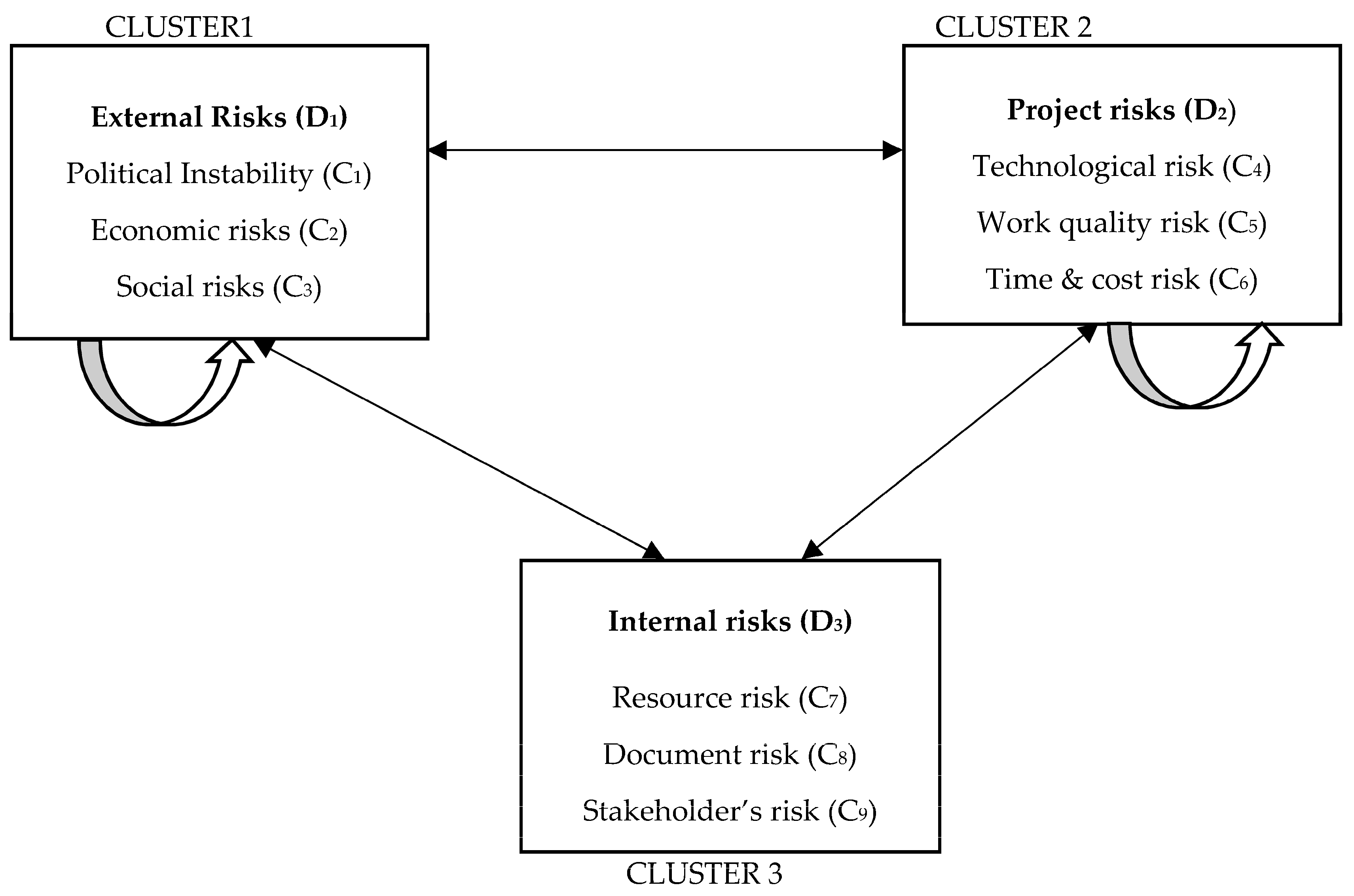
Figure 3.
Network structure among construction risk dimensions and criteria.

Figure 4.
D numbers based Multi-Attributive Border Approximation area Comparison (D-MABAC) in risk mitigation strategy selection.
Figure 4.
D numbers based Multi-Attributive Border Approximation area Comparison (D-MABAC) in risk mitigation strategy selection.

Figure 5.
Sensivity analysis of the alternative ranking through different scenarios.


Table 1.
Summary of demographic profile of respondents.
| Characteristics | Frequency | Percentage (%) | |
|---|---|---|---|
| Age group | 21–31 | 2 | 20 |
| 31–39 | 4 | 40 | |
| 39–45 | 3 | 30 | |
| 45–58 | 1 | 10 | |
| Gender | Female | 4 | 40 |
| Male | 6 | 60 | |
| Level of Education | Bachelor’s degree | 4 | 40 |
| Master’s degree | 5 | 50 | |
| Higher | 1 | 10 | |
| Role of respondents | Chief personal officer | 1 | 10 |
| Manager or general manager | 2 | 20 | |
| Staff or assistant manager | 1 | 10 | |
| Project risks analyst | 2 | 20 | |
| Purchasing manager | 1 | 10 | |
| Construction site engineer | 3 | 30 | |
| Years of experience in construction sector | Above 15 years | 2 | 20 |
| 10 years~15 years | 4 | 40 | |
| 5 years~10 years | 3 | 30 | |
| Less than 5 years | 1 | 10 | |
| Total available number | 10 |
Table 2.
Risk factors involved in construction projects.
| Risk Indicators in Project Based Construction Management | References |
|---|---|
| Environmental risk; political, social and economic risk; contractual agreement risk; financial risk; construction risk; project design risk; market risk. | [1] |
| Safety risk, quality risk, environmental risk, political risk, project site risk, project complexity risk. | [53] |
| Quality risks, personnel risks, cost risks, deadline risks, strategic decision risks, external risks. | [17] |
| Operational risk, economic risk, political risk, financial risk, legal risk, currency and inflation risk, corruption risk, tendering procedures. | [3] |
| Political risks, economic risk, social risk, weather risk, cost, quality risk, technical risk, construction risk, resources risk, project member risk, information risk, construction site risks. | [23] |
| Resources risk, inexperience of project members, lack of motivational approach, design errors risk, efficiency risk, technical risk, quality risk. | [21] |
| Inflation risk, Payment security risk, Programme overrun risk, subcontractor pricing risk. | [56] |
| Political risk, economic risk, natural risk, legal risk, contractor risk, financial risk, management risk, equipment risk, designer risk. | [25] |
| Management risk, project risk, design risk, financial risk, operational risk, external risk. | [14] |
| Information risk, cost risks, lack of coordination, project schedule risk, lack of professional planning, legal dispute risk. | [15] |
| Designing risk, time risk, budget risk, labour risk, political risk. | [16] |
| Design risk, payment delay risk, funding risk, quality risk, labour dispute risks, natural disaster risk, exchange rate fluctuation risk, political instability, site condition risks, insurance inadequacy risk. | [9] |
| Technical risks, organisational risks, socio-political risks, environmental risks, financial risks. | [6] |
| Inflation (economic) risk, environmental and geological risk, design risk, construction delay risk, inadequate managerial skills risk, resource risk. | [29] |
Table 3.
Dimensions and risk criteria involved in construction projects.
| Risk Dimension | Risk Criteria * | Brief Descriptions of Causes of the Mentioned Criteria Risks |
|---|---|---|
| External risks (D1) | Political instability (C1) | Frequent changes in government due to disputes among political parties, change in law due to local government’s unpredictable new regulations, needless influence by local government on court proceedings regarding project disputes. |
| Economic risk (C2) | Fluctuation in currency exchange rate, unpredictable inflation due to immature banking systems, payment delays due to poor funding for project, inadequate forecasting about market demand. | |
| Social risk (C3) | Racial tension and differences in work culture and language between foreign and local partners. | |
| Project risk (D2) | Technological risk (C4) | Risk of insufficient technology, improper design, unexpected design changes; inadequate site investigation; change in construction procedures and insufficient resource availability. |
| Work quality risk (C5) | Corruption, including bribery, at sites; obsolete technology and practices by the local partner; low local workforce labor productivity due to poor skills or inadequate supervision; improper quality control; local partner tolerance of defects and inferior quality. | |
| Time and cost risk (C6) | Delays due to disputes with contractors, natural disasters, and lack of availability of utilities; risk of labor disputes and strikes; insufficient cash flow, improper measurements, ill planned schedules, and delays in payment; lack of proper benchmarking and monitoring of construction activities. | |
| Internal risks (D3) | Resource risk (C7) | Difficulty in hiring suitable skilled employees; risk of defective material from suppliers; risk of labor, materials, and equipment availability; poor competence and productivity of labor *. |
| Documents and information risk (C8) | Intellectual property protection risk from former local employees, partners, and third parties; corporate fraud including unexpected increases in turnover, unexpected resignations of financial advisers, intentional or unintentional negligence by auditors, bankers, or creditors. | |
| Stakeholder’s risk (C9) | Local partner’s creditworthiness: Information on local partner’s accounts lucidity, financial soundness, foreign exchange liquidity, staff reliability. Termination of joint ventures (JV): unfair dividends, e.g., assets, shares, and benefits, to foreign firms by local partner upon termination of JV contract. |
Table 4.
Construction risks response strategies.
| Alternative (s) | Preventive Management Techniques | References |
|---|---|---|
| A1 | Proper scheduling for getting updated project information. | [9] |
| A2 | Adjust plans for scope of work and estimates to counter risk implications. | [2] |
| A3 | Get information about local partner’s credibility from present and past business partners. | [4] |
| A4 | Transfer or share risks to/with other parties. | [6] |
| A5 | Merger and diversification of projects. | [23] |
Table 5.
Unweighted supermatrix formed from every risk factor.
| External Risk (D1) | Project Risk (D2) | Internal Risk (D3) | ||||||||
|---|---|---|---|---|---|---|---|---|---|---|
| C1 | C2 | C3 | C4 | C5 | C6 | C7 | C8 | C9 | ||
| External risk (D1) | C1 | 0.000 | 0.576 | 0.589 | 0.315 | 0.386 | 0.373 | 0.332 | 0.353 | 0.395 |
| C2 | 0.525 | 0.000 | 0.411 | 0.357 | 0.351 | 0.347 | 0.336 | 0.321 | 0.327 | |
| C3 | 0.475 | 0.424 | 0.000 | 0.327 | 0.264 | 0.280 | 0.332 | 0.326 | 0.278 | |
| Project risk (D2) | C4 | 0.288 | 0.355 | 0.354 | 0.000 | 0.461 | 0.510 | 0.348 | 0.346 | 0.340 |
| C5 | 0.416 | 0.320 | 0.338 | 0.481 | 0.000 | 0.490 | 0.334 | 0.361 | 0.363 | |
| C6 | 0.296 | 0.326 | 0.308 | 0.519 | 0.539 | 0.000 | 0.318 | 0.293 | 0.298 | |
| Internal risk (D3) | C7 | 0.332 | 0.324 | 0.357 | 0.364 | 0.313 | 0.370 | 0.000 | 1.000 | 1.000 |
| C8 | 0.351 | 0.369 | 0.351 | 0.343 | 0.371 | 0.351 | 1.000 | 0.000 | 1.000 | |
| C9 | 0.316 | 0.308 | 0.292 | 0.293 | 0.315 | 0.279 | 1.000 | 1.000 | 0.000 | |
Table 6.
Inner dependence matrix of construction project factors.
| Dimensions | |||
|---|---|---|---|
| External Risk | Project Risk | Internal Risk | |
| External risk | 1 | 0.518 | 0.503 |
| Project risk | 0.537 | 1 | 0.496 |
| Internal risk | 0.462 | 0.482 | 1 |
Table 7.
Weighted supermatrix based on supply chain risk factors.
| External Risk | Project Risk | Internal Risk | ||||||||
|---|---|---|---|---|---|---|---|---|---|---|
| C1 | C2 | C3 | C4 | C5 | C6 | C7 | C8 | C9 | ||
| External risk | C1 | 0.000 | 0.576 | 0.589 | 0.163 | 0.200 | 0.193 | 0.167 | 0.178 | 0.199 |
| C2 | 0.525 | 0.000 | 0.411 | 0.185 | 0.182 | 0.180 | 0.169 | 0.162 | 0.165 | |
| C3 | 0.475 | 0.424 | 0.000 | 0.170 | 0.137 | 0.145 | 0.167 | 0.164 | 0.140 | |
| Project risk | C4 | 0.155 | 0.191 | 0.191 | 0.000 | 0.461 | 0.510 | 0.173 | 0.172 | 0.169 |
| C5 | 0.223 | 0.172 | 0.182 | 0.481 | 0.000 | 0.490 | 0.166 | 0.179 | 0.180 | |
| C6 | 0.159 | 0.175 | 0.165 | 0.519 | 0.539 | 0.000 | 0.158 | 0.146 | 0.148 | |
| Internal risk | C7 | 0.154 | 0.150 | 0.165 | 0.176 | 0.151 | 0.178 | 0.000 | 1.000 | 1.000 |
| C8 | 0.162 | 0.171 | 0.162 | 0.165 | 0.179 | 0.169 | 1.000 | 0.000 | 1.000 | |
| C9 | 0.146 | 0.142 | 0.135 | 0.141 | 0.152 | 0.134 | 1.000 | 1.000 | 0.000 | |
Table 8.
Normalised weighted supermatrix based on supply chain risk factors.
| External Risk | Project Risk | Internal Risk | ||||||||
|---|---|---|---|---|---|---|---|---|---|---|
| C1 | C2 | C3 | C4 | C5 | C6 | C7 | C8 | C9 | ||
| External risk | C1 | 0.000 | 0.288 | 0.294 | 0.082 | 0.100 | 0.097 | 0.056 | 0.059 | 0.066 |
| C2 | 0.263 | 0.000 | 0.206 | 0.093 | 0.091 | 0.090 | 0.056 | 0.054 | 0.055 | |
| C3 | 0.238 | 0.212 | 0.000 | 0.085 | 0.068 | 0.073 | 0.056 | 0.055 | 0.047 | |
| Project risk | C4 | 0.078 | 0.095 | 0.095 | 0.000 | 0.231 | 0.255 | 0.058 | 0.057 | 0.056 |
| C5 | 0.112 | 0.086 | 0.091 | 0.241 | 0.000 | 0.245 | 0.055 | 0.060 | 0.060 | |
| C6 | 0.079 | 0.088 | 0.083 | 0.260 | 0.270 | 0.000 | 0.053 | 0.049 | 0.049 | |
| Internal risk | C7 | 0.077 | 0.075 | 0.083 | 0.088 | 0.075 | 0.089 | 0.000 | 0.333 | 0.333 |
| C8 | 0.081 | 0.085 | 0.081 | 0.083 | 0.090 | 0.085 | 0.333 | 0.000 | 0.333 | |
| C9 | 0.073 | 0.071 | 0.068 | 0.071 | 0.076 | 0.067 | 0.333 | 0.333 | 0.000 | |
Table 9.
Limited supermatrix based on supply chain risk factors.
| External Risk | Project Risk | Disruption Risk | ||||||||
|---|---|---|---|---|---|---|---|---|---|---|
| C1 | C2 | C3 | C4 | C5 | C6 | C7 | C8 | C9 | ||
| External risk | C1 | 0.1062 | 0.1062 | 0.1062 | 0.1062 | 0.1062 | 0.1062 | 0.1062 | 0.1062 | 0.1062 |
| C2 | 0.0958 | 0.0958 | 0.0958 | 0.0958 | 0.0958 | 0.0958 | 0.0958 | 0.0958 | 0.0958 | |
| C3 | 0.0894 | 0.0894 | 0.0894 | 0.0894 | 0.0894 | 0.0894 | 0.0894 | 0.0894 | 0.0894 | |
| Project risk | C4 | 0.0972 | 0.0972 | 0.0972 | 0.0972 | 0.0972 | 0.0972 | 0.0972 | 0.0972 | 0.0972 |
| C5 | 0.0996 | 0.0996 | 0.0996 | 0.0996 | 0.0996 | 0.0996 | 0.0996 | 0.0996 | 0.0996 | |
| C6 | 0.0971 | 0.0971 | 0.0971 | 0.0971 | 0.0971 | 0.0971 | 0.0971 | 0.0971 | 0.0971 | |
| Internal risk | C7 | 0.1392 | 0.1392 | 0.1392 | 0.1392 | 0.1392 | 0.1392 | 0.1392 | 0.1392 | 0.1392 |
| C8 | 0.1406 | 0.1406 | 0.1406 | 0.1406 | 0.1406 | 0.1406 | 0.1406 | 0.1406 | 0.1406 | |
| C9 | 0.1349 | 0.1349 | 0.1349 | 0.1349 | 0.1349 | 0.1349 | 0.1349 | 0.1349 | 0.1349 | |
Table 10.
Ranking of construction project risk criteria.
| Dimensions | Risk Criteria | Ranking |
|---|---|---|
| External risk (D1) | Political instability (C1) | 4 |
| Economic risk (C2) | 8 | |
| Social risk (C3) | 9 | |
| Project risk (D2) | Technological risk (C4) | 6 |
| Work quality risk (C5) | 5 | |
| Time and cost risk (C6) | 7 | |
| Internal risk (D3) | Resource risk (C7) | 2 |
| Document and information risk (C8) | 1 | |
| Stakeholder’s risk (C9) | 3 |
Table 11.
Comparison of alternatives w.r.t risk criteria using D numbers.
| C1 | C2 | C3 | C4 | C5 | C6 | C7 | C8 | C9 | |
|---|---|---|---|---|---|---|---|---|---|
| A1 | (0.62, 0.5) | (0.72, 0.4), (0.48, 0.6) | (0.53, 0.4) | (0.58, 0.5) | (0.72, 0.6) | (0.48, 0.6), (0.64, 0.4) | (0.66, 0.6) | (0.38, 0.9) | (0.84, 0.2) |
| A2 | (0.68, 0.4) | (0.44, 0.8) | (0.64, 0.6), (0.32, 0.3) | (0.44,.9) | (0.82, 0.9) | (0.88, 0.6) | (0.56, 0.8) | (0.92, 0.8) | (0.69, 0.4) |
| A3 | (0.54, 0.8), (0.68, 0.2) | (0.68, 0.3) | (0.47, 0.9) | (0.78, 0.8) | (0.38, 0.7), (0.59, 0.3) | (0.68, 0.5) | (0.29, 0.6), (0.39, 0.4) | (0.28, 0.6) | (0.34, 0.6) |
| A4 | (0.72, 0.9) | (0.49, 0.7) | (0.78, 0.4) | (0.86, 0.4) | (0.88, 0.4) | (0.47, 0.7) | (0.64, 0.2) | (0.62, 1) | (0.56, 0.7) |
| A5 | (0.48, 1) | (0.56, 0.9) | (0.82, 0.7) | (0.36, 1) | (0.78, 0.7) | (0.59, 0.9) | (0.78, 0.7) | (0.68, 0.3), (0.49, 0.6) | (0.44, 0.8) |
Table 12.
Normalised decision matrix of alternatives w.r.t criteria.
| C1 | C2 | C3 | C4 | C5 | C6 | C7 | C8 | C9 | |
|---|---|---|---|---|---|---|---|---|---|
| A1 | 0.8989 | 0 | 1 | 1 | 0.7927 | 0 | 0.3589 | 0.5846 | 1 |
| A2 | 1 | 0.6022 | 0.2597 | 0.6826 | 0 | 0.0744 | 0.2344 | 0 | 0.5179 |
| A3 | 0.2128 | 1 | 0.4171 | 0 | 0.7642 | 0.9488 | 0.5167 | 0.8427 | 0.8393 |
| A4 | 0 | 0.6263 | 0.7238 | 0.8383 | 1 | 1 | 1 | 1 | 0 |
| A5 | 0.4468 | 0.1935 | 0 | 0.7904 | 0.4974 | 0.0605 | 0 | 0.3531 | 0.1786 |
Table 13.
Weighted normalised decision matrix of alternatives w.r.t criteria.
| C1 | C2 | C3 | C4 | C5 | C6 | C7 | C8 | C9 | |
|---|---|---|---|---|---|---|---|---|---|
| A1 | 0.2017 | 0.1916 | 0.1788 | 0.1944 | 0.1786 | 0.0971 | 0.1892 | 0.2381 | 0.2698 |
| A2 | 0.2124 | 0.1304 | 0.1126 | 0.1636 | 0.0996 | 0.1043 | 0.1718 | 0.1406 | 0.2048 |
| A3 | 0.1288 | 0.1641 | 0.1267 | 0.0972 | 0.1757 | 0.1892 | 0.2111 | 0.2812 | 0.2481 |
| A4 | 0.1062 | 0.1324 | 0.1541 | 0.1787 | 0.1992 | 0.1942 | 0.2784 | 0.1693 | 0.1349 |
| A5 | 0.1537 | 0.0958 | 0.0894 | 0.1740 | 0.1491 | 0.1030 | 0.1392 | 0.1995 | 0.1590 |
Table 14.
Ranking of alternatives using the D-MABAC method.
| Alternative Risk Responses | Q | Rank | |
|---|---|---|---|
| Risk response (A1) | Proper scheduling for getting updated project information. | 0.2830 | 1 |
| Risk response (A2) | Adjust plans for scope of work and estimates to counter risk implications. | −0.1161 | 4 |
| Risk response (A3) | Get information about local partner’s credibility from its present and past business partners. | 0.1660 | 2 |
| Risk response (A4) | Transfer or share risks to/with other parties. | 0.0913 | 3 |
| Risk response (A5) | Merger and diversification of projects. | −0.1935 | 5 |
Table 15.
Comparison of MABAC with various existing multi-criteria decision making methods.
| Alternative Risk Responses | D-MABAC | D-TOPSIS | D-COPRAS | D-ARAS |
|---|---|---|---|---|
| A1 | 1 | 1 | 1 | 1 |
| A2 | 4 | 4 | 4 | 4 |
| A3 | 2 | 2 | 2 | 2 |
| A4 | 3 | 3 | 3 | 3 |
| A5 | 5 | 5 | 5 | 5 |
Table 16.
Rank correlation of various MCDM methods.
| Spearman’s Coefficient | D-MABAC | D-TOPSIS | D-COPRAS | D-ARAS |
|---|---|---|---|---|
| - | 1.000 | 1.000 | 1.000 |
Table 17.
Scenarios for different criteria weights.
| Scenarios * | ||||||||
|---|---|---|---|---|---|---|---|---|
| Criteria | S1 | S2 | S3 | S4 | S5 | S6 | S7 | S8 |
| C1 | 0.0113 | 0.1482 | 0.0226 | 0.2674 | 0.1944 | 0.0795 | 0.0081 | 0.1602 |
| C2 | 0.1578 | 0.1121 | 0.1204 | 0.1178 | 0.0914 | 0.0632 | 0.0962 | 0.0537 |
| C3 | 0.0576 | 0.1789 | 0.2946 | 0.0001 | 0.1853 | 0.0577 | 0.0308 | 0.1054 |
| C4 | 0.0904 | 0.1118 | 0.2655 | 0.1556 | 0.2219 | 0.0519 | 0.2032 | 0.0958 |
| C5 | 0.1172 | 0.0033 | 0.0478 | 0.0598 | 0.0603 | 0.0703 | 0.0875 | 0.1805 |
| C6 | 0.2016 | 0.0233 | 0.0496 | 0.0631 | 0.0322 | 0.3311 | 0.1958 | 0.0218 |
| C7 | 0.0894 | 0.1663 | 0.0352 | 0.0937 | 0.056 | 0.0055 | 0.1485 | 0.0223 |
| C8 | 0.2103 | 0.0933 | 0.003 | 0.0276 | 0.0871 | 0.332 | 0.1191 | 0.0539 |
| C9 | 0.0645 | 0.1628 | 0.1613 | 0.215 | 0.0714 | 0.0089 | 0.1107 | 0.3063 |
* Priority criteria are indicated in bold text for different scenarios.
Table 18.
Sensitivity in alternative rankings for different scenarios of criteria weighting.
| Alternative Risk Responses | Scenarios | |||||||
|---|---|---|---|---|---|---|---|---|
| S1 | S2 | S3 | S4 | S5 | S6 | S7 | S8 | |
| A1 | 2 | 1 | 1 | 1 | 1 | 3 | 2 | 1 |
| A2 | 5 | 4 | 4 | 2 | 3 | 5 | 4 | 3 |
| A3 | 1 | 2 | 3 | 3 | 4 | 1 | 3 | 2 |
| A4 | 3 | 3 | 2 | 4 | 2 | 2 | 1 | 4 |
| A5 | 4 | 5 | 5 | 5 | 5 | 4 | 5 | 5 |
© 2018 by the authors. Licensee MDPI, Basel, Switzerland. This article is an open access article distributed under the terms and conditions of the Creative Commons Attribution (CC BY) license (http://creativecommons.org/licenses/by/4.0/).
Share and Cite
MDPI and ACS Style
Chatterjee, K.; Zavadskas, E.K.; Tamošaitienė, J.; Adhikary, K.; Kar, S. A Hybrid MCDM Technique for Risk Management in Construction Projects. Symmetry 2018, 10, 46. https://doi.org/10.3390/sym10020046
AMA Style
Chatterjee K, Zavadskas EK, Tamošaitienė J, Adhikary K, Kar S. A Hybrid MCDM Technique for Risk Management in Construction Projects. Symmetry. 2018; 10(2):46. https://doi.org/10.3390/sym10020046
Chicago/Turabian StyleChatterjee, Kajal, Edmundas Kazimieras Zavadskas, Jolanta Tamošaitienė, Krishnendu Adhikary, and Samarjit Kar. 2018. "A Hybrid MCDM Technique for Risk Management in Construction Projects" Symmetry 10, no. 2: 46. https://doi.org/10.3390/sym10020046
Note that from the first issue of 2016, this journal uses article numbers instead of page numbers. See further details here.