Diagonally Implicit Multistep Block Method of Order Four for Solving Fuzzy Differential Equations Using Seikkala Derivatives


1
Institute for Mathematical Research, Universiti Putra Malaysia, Serdang 43400, Selangor, Malaysia
2
Department of Mathematics, Faculty of Science, Universiti Putra Malaysia, Serdang 43400, Selangor, Malaysia
3
Department of Mathematics and Statistics, Faculty of Applied Science and Technology, Universiti Tun Hussein Onn Malaysia (Pagoh Campus), Muar 84000, Johor, Malaysia
*
Author to whom correspondence should be addressed.
Symmetry 2018, 10(2), 42; https://doi.org/10.3390/sym10020042
Submission received: 31 October 2017
/
Revised: 22 December 2017
/
Accepted: 8 January 2018
/
Published: 8 February 2018
(This article belongs to the Special Issue Fuzzy Sets Theory and Its Applications)
Abstract
:In this paper, the solution of fuzzy differential equations is approximated numerically using diagonally implicit multistep block method of order four. The multistep block method is well known as an efficient and accurate method for solving ordinary differential equations, hence in this paper the method will be used to solve the fuzzy initial value problems where the initial value is a symmetric triangular fuzzy interval. The triangular fuzzy number is not necessarily symmetric, however by imposing symmetry the definition of a triangular fuzzy number can be simplified. The symmetric triangular fuzzy interval is a triangular fuzzy interval that has same left and right width of membership function from the center. Due to this, the parametric form of symmetric triangular fuzzy number is simple and the performing arithmetic operations become easier. In order to interpret the fuzzy problems, Seikkala’s derivative approach is implemented. Characterization theorem is then used to translate the problems into a system of ordinary differential equations. The convergence of the introduced method is also proved. Numerical examples are given to investigate the performance of the proposed method. It is clearly shown in the results that the proposed method is comparable and reliable in solving fuzzy differential equations.
1. Introduction
Modeling of real-world problems involves ordinary differential equations (ODEs) that are not always perfect. For example, the initial value may not be known exactly and the function may contain uncertain parameters. This inexactness leads to the necessity of fuzzy differential equations (FDEs) to overcome the situation. Examples of FDEs application in real life include models such as in solid waste management systems [1], hydraulic differential servo cylinders [2], population models [3], hyperchaotic systems [4], and service composition [5].
Chang and Zadeh in [6] first introduced the fuzzy derivative concept. The concept was then extended by Dubois and Prade [7] and the authors also addressed the problem of linearity. Goetschel and Voxman [8] and Puri and Ralescu [9] studied and proposed several important definitions and theorems in the fuzzy derivative. A significant contribution for fuzzy initial value problems (FIVPs) is done by Seikkala [10] and Kaleva [11,12].
The exact solutions for certain FDEs are inconvenient and tedious to determine because of the complexity of the FDE problems. Therefore, numerical methods are used for solving the FDEs. Ma et al. in [13] contribute an important work in solving FDEs by using a numerical method. They adopted classical Euler’s method and solve the FIVPs.
Several researchers discussed predictor–corrector methods for solving FDEs [14,15,16,17]. Allahviranloo et al. in [15] developed a predictor–corrector method based on the Adams-Bashforth three-step method as a predictor and the Adams-Moulton two-step method as a corrector. The improvise method of [15] is then proposed in [14]. Shang and Guo [17] derived the predictor–corrector method based on Adams-Bashforth four-step method and the Adams-Moulton three-step method as a predictor and corrector respectively. Jayakumar [16] introduced Adams fifth order predictor–corrector method for solving FDEs by considering the Adams-Bashforth five-step method as a predictor and the Adam-Moulton four-step method as a corrector. All studies aimed to determine better accuracy and efficiency in finding solutions to FDEs.
The multistep block method is an efficient method for solving ODEs. In this method, several approximation points will be computed simultaneously on the -axis in the block. Mehrkanoon et al. in [18] and Isa and Majid in [19] solved FDEs by using the 2-point fully implicit multistep block method. Diagonally implicit multistep block method is used by Zawawi et al. [20] and Ramli and Majid [21,22] for solving FDEs. Zawawi et al. proposed diagonally implicit block backward differentiation formulas, while Ramli and Majid developed an Adams-type diagonally implicit multistep block method, which considered order four for first point and order five for the second point. Fook and Ibrahim in [23] solved FDEs by using a 2-points hybrid block method.
This paper will discuss the implementation of a 2-point diagonally implicit multistep block method to solve fuzzy differential equations. The method will compute the numerical solutions at two points simultaneously using constant step size. The two formulas of the diagonally implicit block method of Adams type will have the same order for the first and second formula.
This paper is organized as follows. Some basic definitions and notations are in Section 2. Definition of FIVP in Section 3 and description of the 2-point diagonally implicit multistep block method of order four (2PDO4) will be discussed in Section 4. In the next section, the implementation of the block method for solving FIVP and its algorithm is proposed in Section 5 and Section 6 respectively. The convergence of the method is proved in Section 7. Numerical results are provided in Section 8 and conclusion of this study is at the end of the paper.
2. Preliminaries
Some basic definitions and notations that are significant for this paper will be reviewed in this section. For further details, refer [15,24,25,26] (to name a few).
Definition 1.
Let is a mapping of fuzzy number with is set of all real numbers. The mapping has following properties:
- 1.
- upper semicontinuous,
- 2.
- is fuzzy convex, that is, , for all ,
- 3.
- is normal, that is exist such that ,
- 4.
- The support of is and its closure is compact.
Consider as set of all fuzzy numbers on .
Definition 2.
The -level set of a fuzzy number and denoted by , is defined as
and is closed and bounded interval by where and denotes the left-hand endpoint and right-hand endpoint of respectively.
The summation and scalar multiplication in are defined as:
- ,
Given the Hausdorff distance as the distance between two fuzzy numbers and a metric in as follows
with the following properties
- is a complete metric space.
Let be a fuzzy valued function.
Definition 3.
If for arbitrary fixed and such that
is said to be continuous.
Hukuhara differentiability (H-derivative) for fuzzy mappings is introduced by Puri and Ralescu in [9]. The differentiability is based on H-difference sets. Definition 4 and 5 explained the concept.
Definition 4.
Let . If there exist such that , then is called the H-difference of and , and it is denoted by . The sign “” stands for H-difference and note that .
Definition 5.
is differentiable at if exist such that
exist and are equal to .
Here, the limits are taken in the metric space since we have defined and .
3. Fuzzy Initial Value Problems
In this paper, we will consider first order FIVP as follows
where is a fuzzy function of , is a fuzzy function of crisp variable and fuzzy variable , and is Hukuhara fuzzy derivative of with the given initial value . Let , if is Hukuhara differentiable then , and .
The parametric form of is given by
As referred to [21], the Seikkala derivative of a fuzzy function is defined by
provided that the equation defines a fuzzy number.
For solving (1) by using numerical methods for ODEs, it must be translated to system of ODEs. Bede in [27] proposed characterization theorems for the solutions of FDEs by using ODEs.
Theorem 1.
Let be Hukuhara differentiable and denote . Functions and are differentiable and based on Seikkala derivative
Therefore (1) can be translated to the system of ODEs
Theorem 2.
Consider FIVP (1) where such that
- 1.
- ,
- 2.
- and are equicontinuous (that is for any and any we have and for all whenever and uniformly bounded on any bounded set,
- 3.
- there exist an such that, and, .
Then FIVP (1) and the system of ODEs (2) are equivalent.
4. Derivation of 2-Point Diagonally Implicit Multistep Block Method
Consider the initial value problems (IVPs) for ODEs of the form
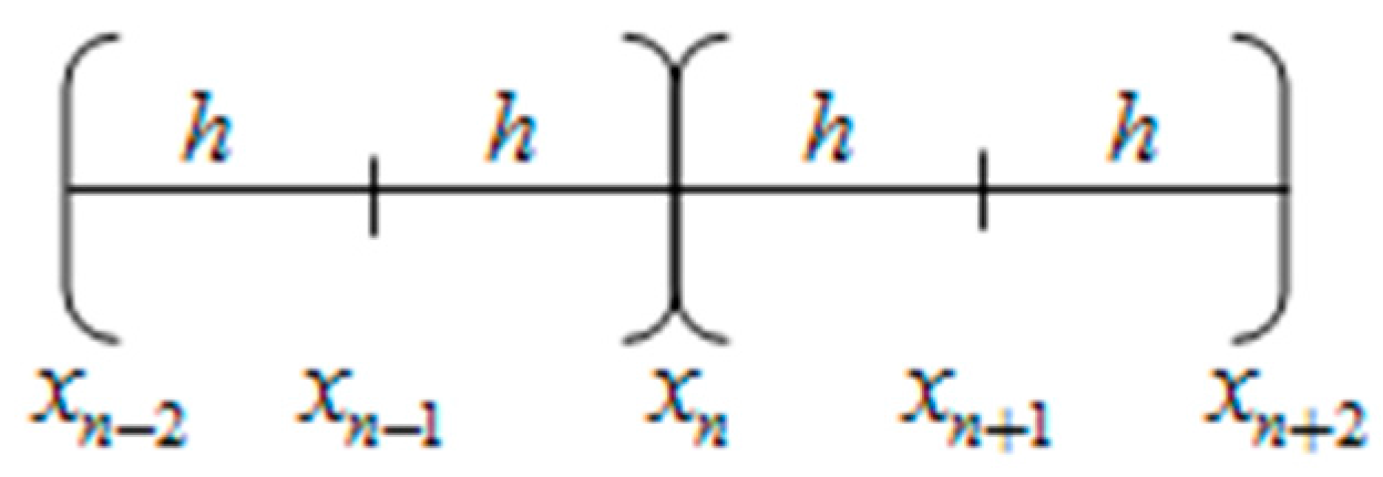
where and are finite. The interval will be divided into a series of blocks. In this proposed method, each block contained two points, and which will be computed simultaneously in a block with the step size at the points and respectively as in Figure 1.
The Lagrange interpolation polynomial is applied for the derivation of predictor and corrector formulas. To obtain the predictor formulas, the set of points is interpolated and the order of the formulas is one less than the corrector formulas. The corrector formulas will use the set of interpolation points i.e., for derivation of and for derivation of . The formulas of will used three back values , while the will used two back values i.e., .
Formulas for and are derived by integrating (3) such that
where the interval of integration for and are and respectively. These are equivalent to
and
The function in (5) and (6) is replaced by the Lagrange polynomial which interpolates the set of corresponding mentioned points. Evaluating the integral in (5) using MAPLE gives the formula for the first and second point of the block multistep method as follows:
The first point,
and the second point,
As referred to [28,29],
form the general matrix of linear multistep method where and are by matrices with elements and for . The associated difference operator is given by
where is the exact solution and assume to be sufficiently differentiable. If , is said to be order and is called the error constant.
The general form of constant is defined as
To determine the order of the method, (7) and (8) is written in matrix form as follows
From (12), and . Hence, by applying (11), and . Since the method is concluded as order four and the error constant is .
5. Implementation for Solving FIVPs
Consider the FIVP (1) and let the exact solution is denoted by while is the approximate solution. To integrate the system (2), from let , and replace by
denoted as the exact solution at , with the approximate solution . Given where and .
The general fuzzy 2PDO4 method by considering (7) and (8) is written as
for the exact solutions and
for the approximate solutions.
6. Algorithm
The following algorithm is based on using 2PDO4 method. To approximate the solution of the following FIVP
For as an arbitrary positive integer,
- Step 1. Let . The initial value is obtained from the FIVP and Runge–Kutta order four is used to determine the two starting points. Hence,
- Step 2. Let .
- Step 3. Let and .
- Step 4. Let the predictor formulas
- Step 5. Let the corrector formulas
- .
- If , go to Step 3.
- Algorithm is completed and approximates .
7. Convergence
From (16) and (17)
are the 2PDO4 method over the interval and approximate to and respectively. Given
is the convergence condition for the approximates. The following lemma is considered to proof the convergence.
Lemma 1.
[9] Let (a sequence of numbers) satisfy:
for some given positive constants and . Then
and
where for all and , and are constants. The proof by using mathematical induction is straightforward.
Theorem 3.
For arbitrary fixed , approximate solutions (16) and (17) converge to the exact solutions and for .
Proof.
By applying (19), it is sufficient to show
Consider the exact solutions (14) and (15), then
where . Therefore, by subtracting (20) and (16), and (21) and (17) yield
and
Denote and . Then (22) and (23) becomes
and
where and .
Consider the first point (24), let , then
are resulted. Let , then by Lemma 1 and (also ):
are obtained. If then and which concludes the proof.
Consider the second point (25), let , then
are resulted. Let , then by Lemma 1 and (also ):
are obtained. If then and which concludes the proof. ☐
Remark 1.
Above theorem results that convergence order is .
8. Results and Discussion
To implement the 2PDO4 method, mode is used where , C and stands for predictor, corrector and evaluation of a function respectively. The implementation is repeated times for each step and step size is considered in the numerical results.
The following FIVPs were tested to show the performance of the proposed method:
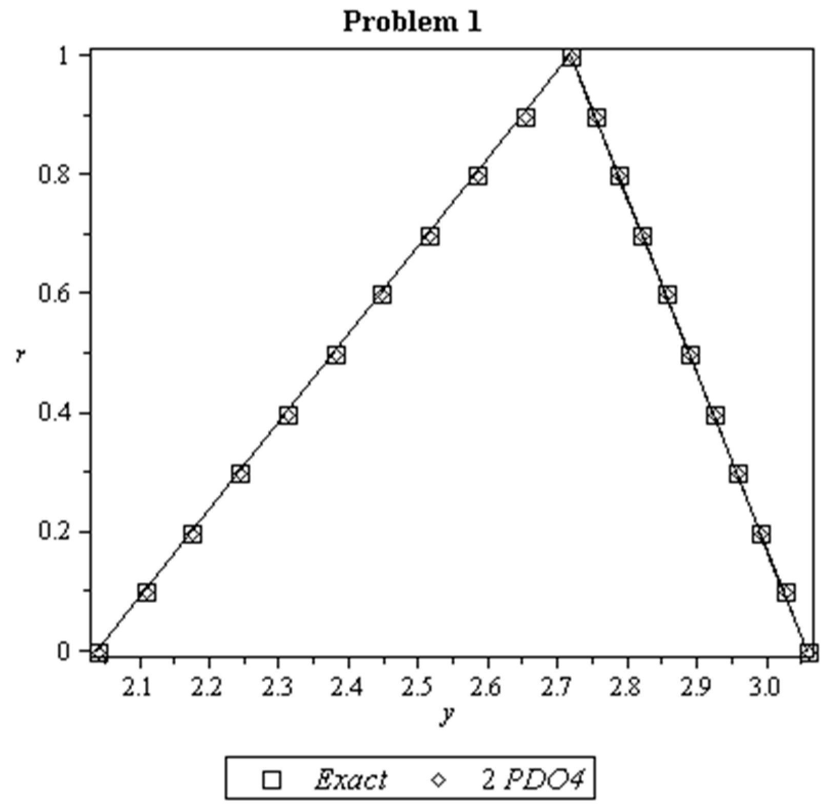
Problem 1.
(Ma et al. [13]) Consider linear FIVP:
Exact solution: .
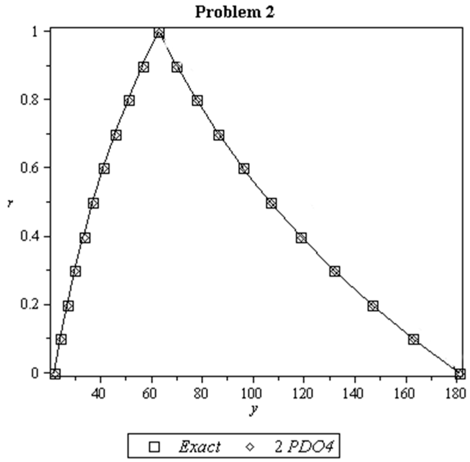
Problem 2.
[ is a triangular fuzzy number where the basis of the membership function of is in the interval with the known summit . Hence, the triangular fuzzy numbers are denoted by ].
Exact solution: .
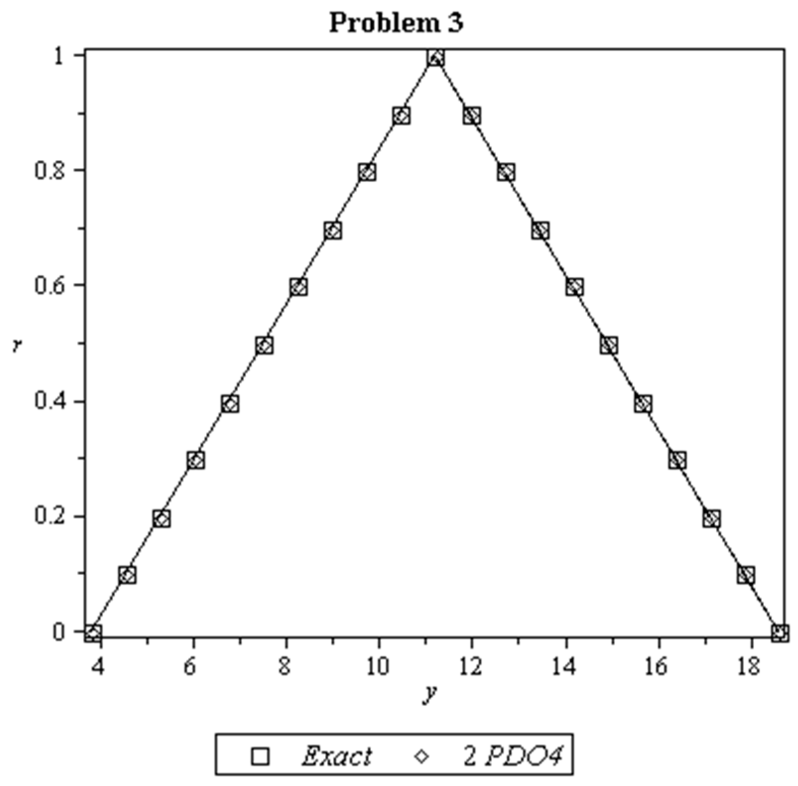
Problem 3.
(Ghanbari [31]) Consider nonlinear FIVP:
Exact solution:
Problem 4.
Exact solution:
Problem 5.
(Ma et al. [13]) Consider nonlinear FIVP:
The following notations are used in the tables:
- : Fuzzy numbers with bounded -level intervals
- : Lower and upper bounded exact solution
- : Lower and upper bounded approximated solution
- FCN: Total function calls
- TS: Total steps taken
- TIME: The execution time taken in seconds
- 2PDO4: 2-point diagonally implicit multistep method of order four
- ERK4: Extended Runge–Kutta-like formulae of order 4 [26]
- RK4: Runge–Kutta method of order 4 [33]
- ANN: Artificial neural network approach [34]
Absolute error is defined as , where , denoted as the exact solutions and as approximate solutions at . The code is written in C language by using Microsoft visual C++ platform.
The numerical results of 2PDO4 compared to ERK4, RK4 and ANN are display in Table 1, Table 2, Table 3, Table 4 and Table 5 when solving Problem 1–5. Note that these results are at with .
From Table 1, Table 2 and Table 3, it is obvious that 2PDO4 gives better results compared to ERK4, RK4 and ANN in terms of accuracy. It is also observed that the execution times of 2PDO4 for solving Problem 3 and 5 are faster than the RK4. Table 4 shows that 2PDO4 used less number of function evaluations to obtain comparable accuracy compared to ERK4 and RK4.
For Problem 5, the exact solutions cannot be calculated analytically. Hence, we compared the approximate solutions of 2PDO4 and RK4. The approximate solutions of Problem 5 at with are presented in Table 5. It can be observed that 2PDO4 is applicable to solve Problem 5 with an advantage of less total steps and faster execution times compared to RK4.
It is obvious in 1−5 that 2PDO4 required less number of total steps compared to other methods. This is expected since 2PDO4 approximates the solutions at two points simultaneously.
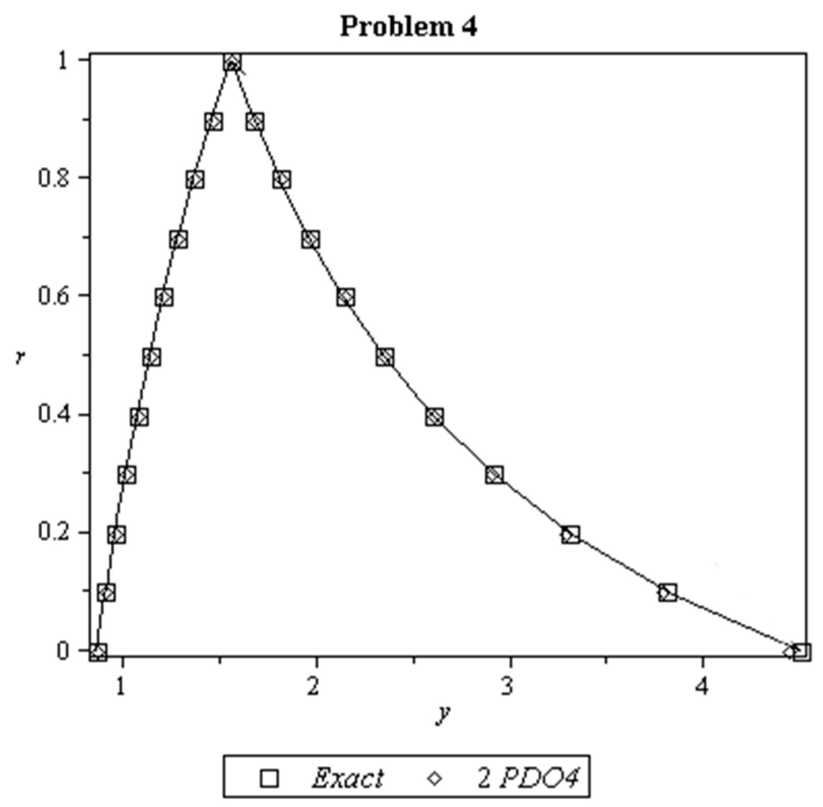
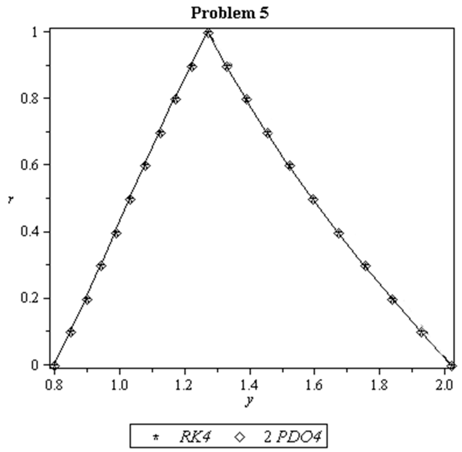
Figure 2, Figure 3, Figure 4 and Figure 5 is a plot of the exact and approximate solutions by using 2PDO4 for Problems 1–4. It is clear in the figures that the solutions by the 2PDO4 method almost coincide with the exact solutions. While the plot of approximate solutions for Problem 5 by using 2PDO4 and RK4 is shown in Figure 6.
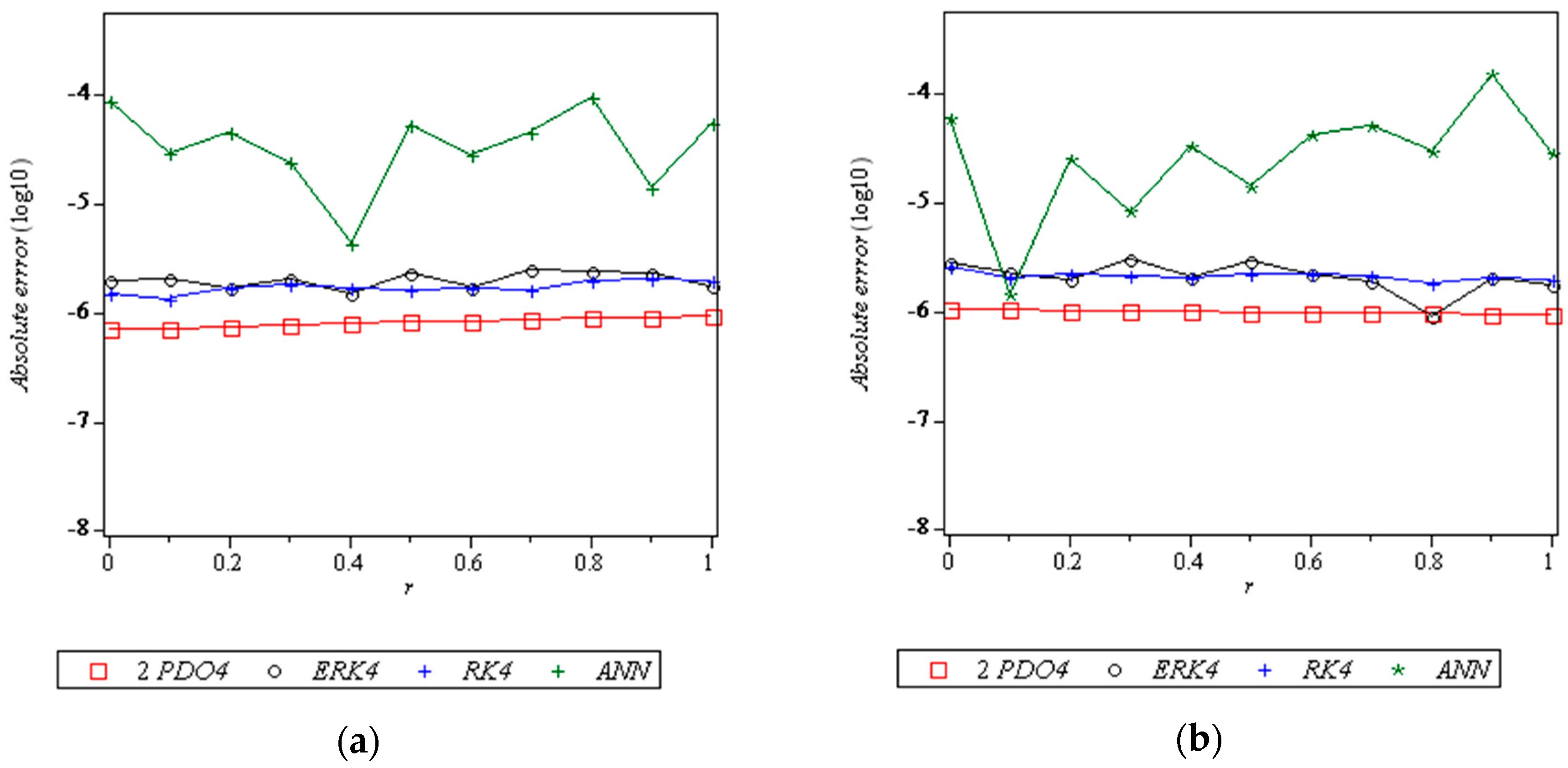
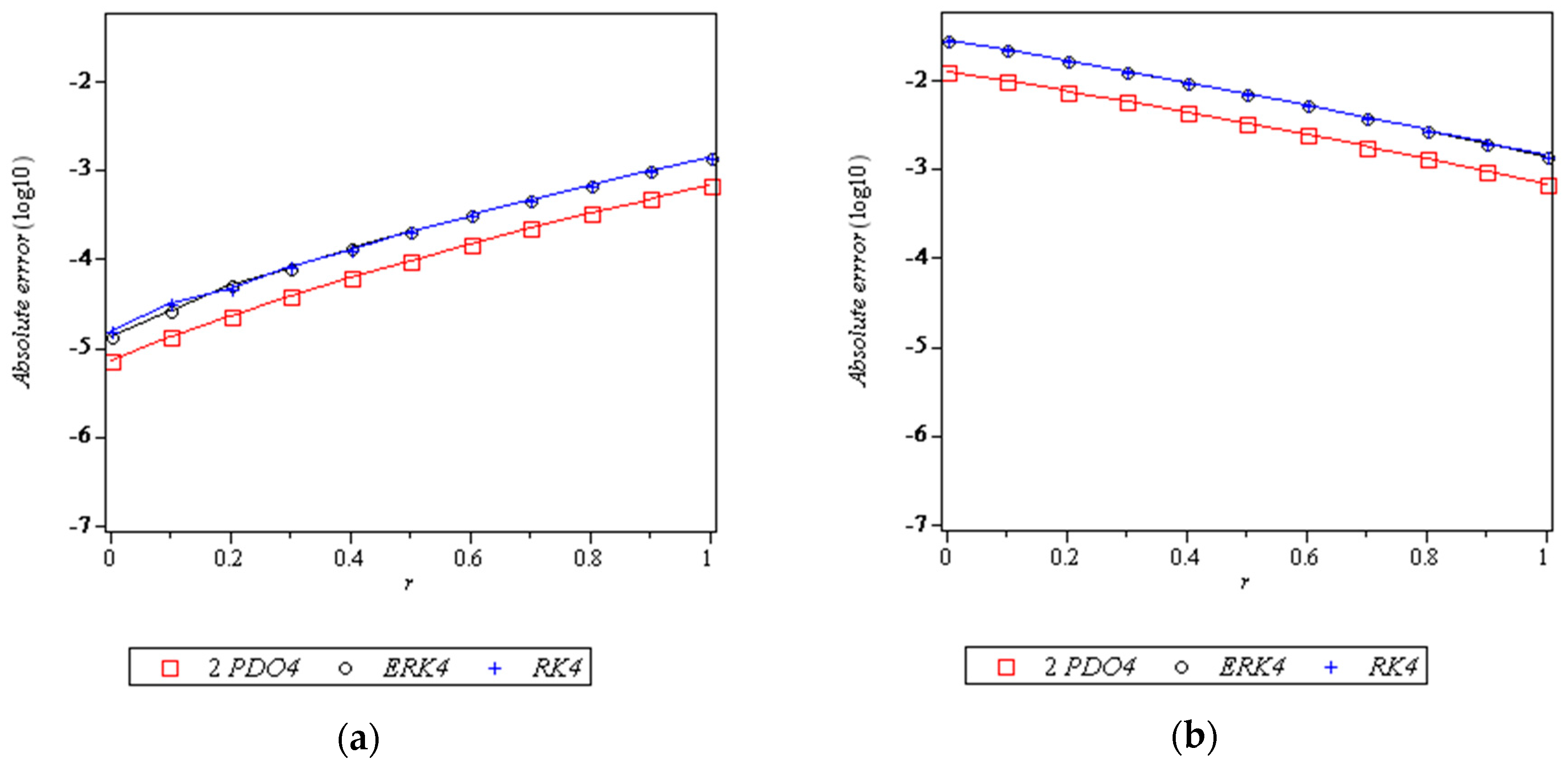
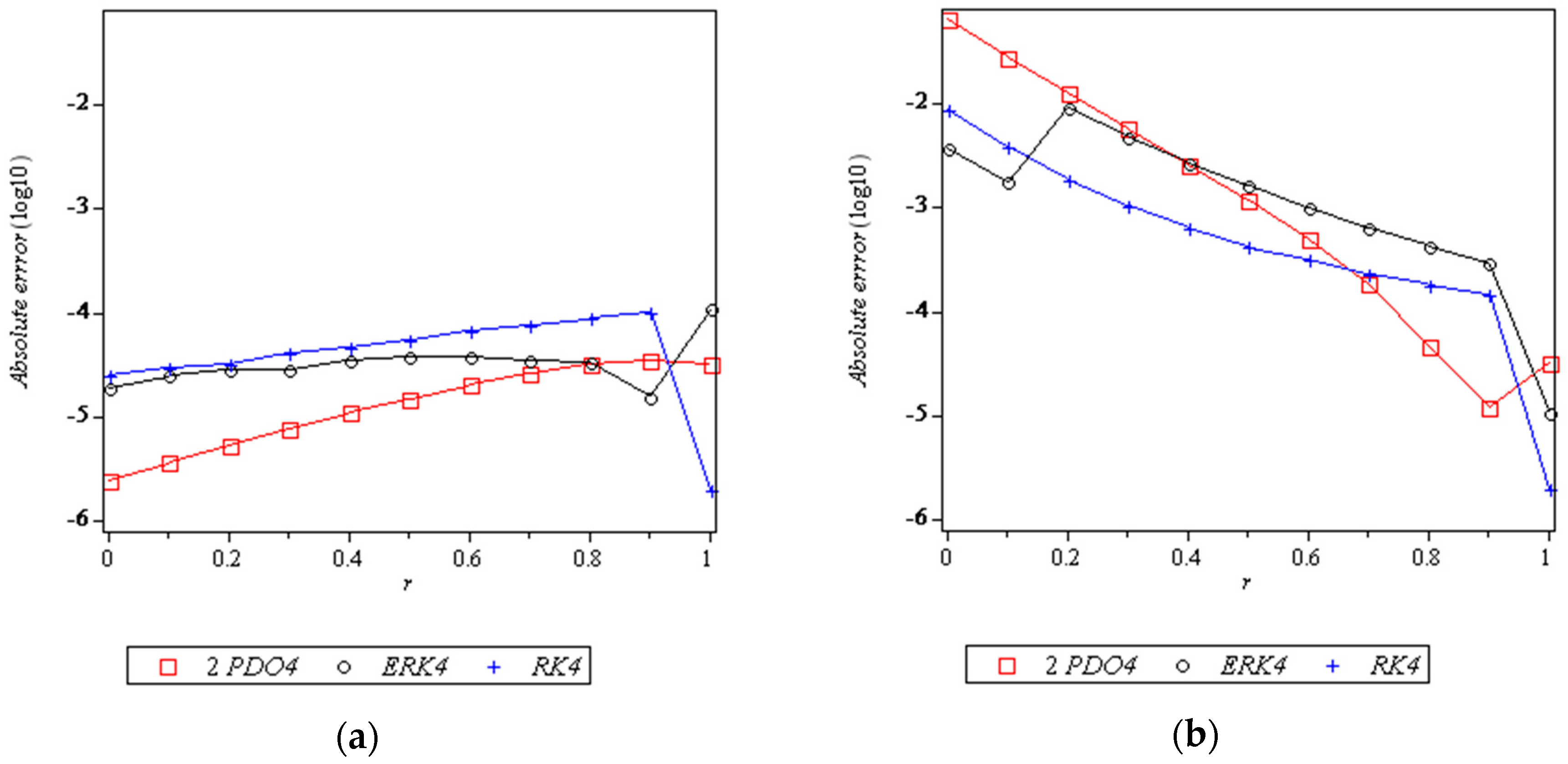
Figure 7, Figure 8, Figure 9 and Figure 10 is a plot of the absolute errors versus for lower and upper bounds of Problems 1–4. It can be seen in Figure 7, Figure 8 and Figure 9 that the errors of 2PDO4 are smaller than the comparison methods, but in Figure 10 the errors of 2PDO4 are smaller at certain points.
9. Conclusions
In this paper, the diagonally implicit block method of order four (2PDO4) has been implemented for solving linear and nonlinear FDEs. Numerical results have shown that the proposed method gave comparable results in terms of accuracy and fewer total steps. The total functions are comparable or less compared to the existing method. The 2PDO4 is able to obtain less execution time than RK4 when solving two tested problems. Hence, the 2PDO4 method can be named in the literature as an additional and reliable method for solving FDEs.
Acknowledgments
Authors gratefully acknowledge the financial support of Research University Grant from Universiti Putra Malaysia and the scholarship of the Academic Training Scheme (SLAI) from Ministry of Higher Education Malaysia.
Author Contributions
Syahirbanun Isa conceived, designed, performed the experiments and wrote the paper. Zanariah Abdul Majid supervised the designed experiments and analyzed the data, Fudziah Ismail and Faranak Rabiei analyzed the data and checking the paper.
Conflicts of Interest
The authors declare that there is no conflict of interests regarding the publication of this paper.
References
- Chen, H.W.; Chang, N.B. Prediction analysis of solid waste generation based on grey fuzzy dynamic modeling. Resour. Conserv. Recycl. 2000, 29, 1–18. [Google Scholar] [CrossRef]
- Bencsik, A.L.; Bede, B.; Tar, J.K.; Fodor, J. Fuzzy differential equations in modeling of hydraulic differential servo cylinders. In Proceedings of the Third Romanian-Hungarian Joint Symposium on Applied Computational Intelligence (SACI), Timisoara, Romania, 25–26 May 2006. [Google Scholar]
- Guo, M.; Xue, X.; Li, R. Impulsive functional differential inclusions and fuzzy population models. Fuzzy Sets Syst. 2003, 138, 601–615. [Google Scholar] [CrossRef]
- Zhang, H.; Liao, X.; Yu, J. Fuzzy modeling and synchronization of hyperchaotic systems. Chaos Solitons Fractals 2005, 26, 835–843. [Google Scholar] [CrossRef]
- Ding, Z.; Shen, H.; Kandel, A. Performance analysis of service composition based on fuzzy differential equations. IEEE Trans. Fuzzy Syst. 2011, 19, 164–178. [Google Scholar] [CrossRef]
- Chang, S.S.L.; Zadeh, L.A. On fuzzy mapping and control. IEEE Trans. Syst. Man Cybern. 1972, 30–34. [Google Scholar] [CrossRef]
- Dubois, D.; Prade, H. Towards fuzzy differential calculus part 3: Differentiation. Fuzzy Sets Syst. 1982, 8, 225–233. [Google Scholar] [CrossRef]
- Goetschel, R.; Voxman, W. Elementary fuzzy calculus. Fuzzy Sets Syst. 1986, 18, 31–43. [Google Scholar] [CrossRef]
- Puri, M.L.; Ralescu, D.A. Differential of fuzzy functions. J. Math. Anal. Appl. 1983, 91, 552–558. [Google Scholar] [CrossRef]
- Seikkala, S. On the fuzzy initial value problem. Fuzzy Sets Syst. 1987, 24, 319–330. [Google Scholar] [CrossRef]
- Kaleva, O. Fuzzy differential equations. Fuzzy Sets Syst. 1987, 24, 301–317. [Google Scholar] [CrossRef]
- Kaleva, O. The cauchy problem for fuzzy differential equations. Fuzzy Sets Syst. 1990, 35, 389–396. [Google Scholar] [CrossRef]
- Ma, M.; Friedman, M.; Kandel, A. Numerical solutions of fuzzy differential equations. Fuzzy Sets Syst. 1999, 105, 133–138. [Google Scholar] [CrossRef]
- Allahviranloo, T.; Abbasbandy, S.; Ahmady, N.; Ahmady, E. Improved predictor-corrector method for solving fuzzy initial value problems. Inf. Sci. 2009, 179, 945–955. [Google Scholar] [CrossRef]
- Allahviranloo, T.; Ahmady, N.; Ahmady, E. Numerical solution of fuzzy differential equations by predictor-corrector method. Inf. Sci. 2007, 177, 1633–1647. [Google Scholar] [CrossRef]
- Jayakumar, T.; Raja, C.; Muthukumar, T. Numerical solution of fuzzy differential equations by Adams fifth order predictor-corrector method. Intern. J. Math. Trends Technol. 2014, 8, 33–50. [Google Scholar]
- Shang, D.; Guo, X. Adams predictor-corrector systems for solving fuzzy differential equations. Math. Probl. Eng. 2013, 2013. [Google Scholar] [CrossRef]
- Mehrkanoon, S.; Suleiman, M.; Majid, Z.A. Block method for numerical solution of fuzzy differential equations. Int. Math. Forum 2009, 4, 2269–2280. [Google Scholar]
- Isa, S.; Majid, Z.A. Numerical solution of fuzzy differential equations by multistep block method. In Proceedings of the 7th International Conference on Research and Educations in Mathematics (ICREM7), Kuala Lumpur, Malaysia, 25–27 August 2015; pp. 113–119. [Google Scholar]
- Zawawi, I.S.M.; Ibrahim, Z.B.; Suleiman, M. Diagonally implicit block backward differentiation formulas for solving fuzzy differential equations. AIP Conf. Proc. 2013, 1522, 681–687. [Google Scholar] [CrossRef]
- Ramli, A.; Majid, Z.A. An implicit multistep block method for fuzzy differential equations. In Proceedings of the 7th International Conference on Research and Educations in Mathematics (ICREM7), Kuala Lumpur, Malaysia, 25–27 August 2015; pp. 81–87. [Google Scholar]
- Ramli, A.; Majid, Z.A. Fourth order diagonally implicit multistep block method for solving fuzzy differential equations. Int. J. Pure Appl. Math. 2016, 107, 635–660. [Google Scholar] [CrossRef]
- Fook, T.K.; Ibrahim, Z.B. Two points hybrid block method for solving first order fuzzy differential equations. J. Soft Comput. Appl. 2016, 2016, 45–53. [Google Scholar] [CrossRef]
- Ahmadian, A.; Suleiman, M.; Salahshour, S. An Operational Matrix Based on Legendre Polynomials for Solving Fuzzy Fractional-Order Differential Equations. Abstr. Appl. Anal. 2013. [Google Scholar] [CrossRef]
- Allahviranloo, T.; Salahshour, S. A new approach for solving first order fuzzy differential equation. In Proceedings of the Information Processing and Management of Uncertainty in Knowledge-Based Systems. Applications, Dortmund, Germany, 28 June 28–2 July 2010; pp. 522–531. [Google Scholar]
- Ghazanfari, B.; Shakerami, A. Numerical solutions of fuzzy differential equations by extended Runge-Kutta-like formulae of order 4. Fuzzy Sets Syst. 2012, 189, 74–91. [Google Scholar] [CrossRef]
- Bede, B. Note on Numerical solutions of fuzzy differential equations by predictor-corrector method. Inf. Sci. 2008, 178, 1917–1922. [Google Scholar] [CrossRef]
- Fatunla, S.O. Block methods for second order ODEs. Int. J. Comput. Math. 1991, 41, 55–63. [Google Scholar] [CrossRef]
- Nasir, N.; Ibrahim, Z.B.; Suleiman, M.B.; Othman, K.I. Fifth order two-point block backward differentiation formulas for solving ordinary differential equations. Appl. Math. Sci. 2011, 5, 3505–3519. [Google Scholar]
- Pallingkinis, S.C.; Papageorgiou, G.; Famelis, I.T. Runge-Kutta methods for fuzzy differential equations. Appl. Math. Comput. 2009, 209, 97–105. [Google Scholar] [CrossRef]
- Ghanbari, M. Numerical solution of fuzzy initial value problems under generalized differentiability by HPM. Int. J. Ind. Math. 2009, 1, 19–39. [Google Scholar]
- Dizicheh, A.K.; Salahshour, S.; Ismail, F.B. A note on “Numerical solutions of fuzzy differential equations by extended Runge-Kutta-like formulae of order 4”. Fuzzy Sets Syst. 2013, 233, 96–100. [Google Scholar] [CrossRef]
- Abbasbandy, S.; Allahviranloo, T. Numerical solution of fuzzy differential equation by Runge-Kutta method. Nonlinear Stud. 2004, 11, 117–129. [Google Scholar] [CrossRef]
- Effati, S.; Pakdaman, M. Artificial neural network approach for solving fuzzy differential equations. Inf. Sci. 2010, 180, 1434–1457. [Google Scholar] [CrossRef]
Figure 1.
2-point implicit multistep block method.

Figure 2.
Exact solutions and approximate solutions for Problem 1 at with .

Figure 3.
Exact solutions and approximate solutions for Problem 2 at with .

Figure 4.
Exact solutions and approximate solutions for Problem 3 at with .

Figure 5.
Exact solutions and approximate solutions for Problem 4 at with .

Figure 6.
2PDO4 solutions and RK4 solutions for Problem 5 at with .

Figure 7.
Graph of the numerical results when solving Problem 1: (a) Graph of absolute errors versus for lower bounds; (b) Graph of absolute errors versus for upper bounds.
Figure 7.
Graph of the numerical results when solving Problem 1: (a) Graph of absolute errors versus for lower bounds; (b) Graph of absolute errors versus for upper bounds.

Figure 8.
Graph of the numerical results when solving Problem 2: (a) Graph of absolute errors versus for lower bounds; (b) Graph of absolute errors versus for upper bounds.
Figure 8.
Graph of the numerical results when solving Problem 2: (a) Graph of absolute errors versus for lower bounds; (b) Graph of absolute errors versus for upper bounds.

Figure 9.
Graph of the numerical results when solving Problem 3: (a) Graph of absolute errors versus for lower bounds; (b) Graph of absolute errors versus for upper bounds.
Figure 9.
Graph of the numerical results when solving Problem 3: (a) Graph of absolute errors versus for lower bounds; (b) Graph of absolute errors versus for upper bounds.

Figure 10.
Graph of the numerical results when solving Problem 4: (a) Graph of absolute errors versus for lower bounds; (b) Graph of absolute errors versus for upper bounds.
Figure 10.
Graph of the numerical results when solving Problem 4: (a) Graph of absolute errors versus for lower bounds; (b) Graph of absolute errors versus for upper bounds.


Table 1.
Numerical results of 2PDO4, ERK4, RK4 and ANN for solving Problem 1.
| 2PDO4 | ERK4 1 | RK4 1 | ANN 1 | |
| 0.0 | 7.112242(-7) | 1.969260(-6) | 1.492423(-6) | 8.862866(-5) |
| 0.1 | 7.349317(-7) | 2.090533(-6) | 1.375277(-6) | 2.941706(-5) |
| 0.2 | 7.586392(-7) | 1.734969(-6) | 1.734969(-6) | 4.646277(-5) |
| 0.3 | 7.823466(-7) | 2.094660(-6) | 1.856242(-6) | 2.449152(-5) |
| 0.4 | 8.060541(-7) | 1.500678(-6) | 1.739096(-6) | 4.445810(-6) |
| 0.5 | 8.297616(-7) | 2.337206(-6) | 1.621951(-6) | 5.440010(-5) |
| 0.6 | 8.534691(-7) | 1.743224(-6) | 1.743224(-6) | 2.835439(-5) |
| 0.7 | 8.771765(-7) | 2.579752(-6) | 1.626078(-6) | 4.669132(-5) |
| 0.8 | 9.008840(-7) | 2.462607(-6) | 1.985770(-6) | 9.726296(-5) |
| 0.9 | 9.245915(-7) | 2.345461(-6) | 2.107043(-6) | 1.421725(-5) |
| 1.0 | 9.482990(-7) | 1.751478(-6) | 1.989897(-6) | 5.582846(-5) |
| 2PDO4 | ERK4 1 | RK4 1 | ANN 1 | |
| 0.0 | 1.066836(-6) | 2.834681(-6) | 2.596262(-6) | 5.994298(-5) |
| 0.1 | 1.054983(-6) | 2.297207(-6) | 2.058788(-6) | 1.465839(-6) |
| 0.2 | 1.043129(-6) | 1.998152(-6) | 2.236570(-6) | 2.598870(-5) |
| 0.3 | 1.031275(-6) | 3.129608(-6) | 2.175934(-6) | 8.511551(-6) |
| 0.4 | 1.019421(-6) | 2.115298(-6) | 2.115298(-6) | 3.403441(-5) |
| 0.5 | 1.007568(-6) | 3.008335(-6) | 2.293079(-6) | 1.444274(-5) |
| 0.6 | 9.957139(-7) | 2.232443(-6) | 2.232443(-6) | 4.208012(-5) |
| 0.7 | 9.838602(-7) | 1.933388(-6) | 2.171806(-6) | 5.160297(-5) |
| 0.8 | 9.720064(-7) | 9.190771(-7) | 1.872751(-6) | 3.012583(-5) |
| 0.9 | 9.601527(-7) | 2.050534(-6) | 2.050534(-6) | 1.543513(-4) |
| 1.0 | 9.482990(-7) | 1.751478(-6) | 1.989897(-6) | 2.817154(-5) |
| FCN | 451 | 451 | 451 | - |
| TS | 66 | 110 | 110 | - |
| TIME | 0.675 | - | - | - |
1 Results of ERK4, RK4 and ANN as referred in [26].
Table 2.
Numerical results of 2PDO4, ERK4 and RK4 for solving Problem 2.
| 2PDO4 | ERK4 1 | RK4 1 | |
| 0.0 | 7.586392(-6) | 1.401183(-5) | 1.591918(-5) |
| 0.1 | 1.366979(-5) | 2.666611(-5) | 3.238815(-5) |
| 0.2 | 2.357892(-5) | 5.232929(-5) | 4.851460(-5) |
| 0.3 | 3.919819(-5) | 8.186697(-5) | 8.377432(-5) |
| 0.4 | 6.313677(-5) | 1.334720(-4) | 1.296573(-4) |
| 0.5 | 9.894536(-5) | 2.104650(-4) | 2.104650(-4) |
| 0.6 | 1.513830(-4) | 3.134706(-4) | 3.134706(-4) |
| 0.7 | 2.267426(-4) | 4.676179(-4) | 4.638032(-4) |
| 0.8 | 3.332447(-4) | 6.934862(-4) | 6.858569(-4) |
| 0.9 | 4.815107(-4) | 9.960255(-4) | 9.960255(-4) |
| 1.0 | 6.851258(-4) | 1.419590(-3) | 1.423405(-3) |
| 2PDO4 | ERK4 1 | RK4 1 | |
| 0.0 | 1.260390(-2) | 2.848404(-2) | 2.849930(-2) |
| 0.1 | 9.798071(-3) | 2.185179(-2) | 2.185179(-2) |
| 0.2 | 7.561266(-3) | 1.664276(-2) | 1.662750(-2) |
| 0.3 | 5.790072(-3) | 1.253006(-2) | 1.257584(-2) |
| 0.4 | 4.397464(-3) | 9.443902(-3) | 9.421014(-3) |
| 0.5 | 3.310672(-3) | 7.054700(-3) | 7.039441(-3) |
| 0.6 | 2.469226(-3) | 5.211172(-3) | 5.211172(-3) |
| 0.7 | 1.823209(-3) | 3.812939(-3) | 3.805309(-3) |
| 0.8 | 1.331682(-3) | 2.773261(-3) | 2.773261(-3) |
| 0.9 | 9.613063(-4) | 1.989020(-3) | 1.996649(-3) |
| 1.0 | 6.851258(-4) | 1.419590(-3) | 1.423405(-3) |
| FCN | 451 | 451 | 451 |
| TS | 66 | 110 | 110 |
| TIME | 0.639 | - | - |
1 Results of ERK4 and RK4 as referred in [26].
Table 3.
Numerical results of 2PDO4 and RK4 for solving Problem 3.
| 2PDO4 | RK4 | |
| 0.0 | 6.963978(-5) | 1.010956(-4) |
| 0.1 | 7.770009(-5) | 1.177814(-4) |
| 0.2 | 8.576039(-5) | 1.344671(-4) |
| 0.3 | 9.382069(-5) | 1.511528(-4) |
| 0.4 | 1.018810(-4) | 1.678386(-4) |
| 0.5 | 1.099413(-4) | 1.845243(-4) |
| 0.6 | 1.180016(-4) | 2.012100(-4) |
| 0.7 | 1.260619(-4) | 2.178957(-4) |
| 0.8 | 1.341222(-4) | 2.345815(-4) |
| 0.9 | 1.421825(-4) | 2.512672(-4) |
| 1.0 | 1.502428(-4) | 2.679529(-4) |
| 2PDO4 | RK4 | |
| 0.0 | 2.308459(-4) | 4.348102(-4) |
| 0.1 | 2.227856(-4) | 4.181245(-4) |
| 0.2 | 2.147253(-4) | 4.014387(-4) |
| 0.3 | 2.066649(-4) | 3.847530(-4) |
| 0.4 | 1.986046(-4) | 3.680673(-4) |
| 0.5 | 1.905443(-4) | 3.513816(-4) |
| 0.6 | 1.824840(-4) | 3.346958(-4) |
| 0.7 | 1.744237(-4) | 3.180101(-4) |
| 0.8 | 1.663634(-4) | 3.013244(-4) |
| 0.9 | 1.583031(-4) | 2.846386(-4) |
| 1.0 | 1.502428(-4) | 2.679529(-4) |
| FCN | 451 | 451 |
| TS | 66 | 110 |
| TIME | 0.530 | 0.718 |
Note: Simulation results of 2PDO4 and RK4 have been obtained in the same platform.
Table 4.
Numerical results of 2PDO4, ERK4 and RK4 for solving Problem 4.
| 2PDO4 | ERK4 1 | RK4 1 | |
| 0.0 | 2.459944(-6) | 1.9100(-5) | 2.6100(-5) |
| 0.1 | 3.707531(-6) | 2.5100(-5) | 3.0000(-5) |
| 0.2 | 5.461503(-6) | 2.9100(-5) | 3.2200(-5) |
| 0.3 | 7.872724(-6) | 2.9000(-5) | 4.2000(-5) |
| 0.4 | 1.110316(-5) | 3.5000(-5) | 4.8000(-5) |
| 0.5 | 1.529207(-5) | 3.8000(-5) | 5.5000(-5) |
| 0.6 | 2.047821(-5) | 3.9000(-5) | 6.8000(-5) |
| 0.7 | 2.643397(-5) | 3.5000(-5) | 7.6000(-5) |
| 0.8 | 3.232537(-5) | 3.4000(-5) | 8.9000(-5) |
| 0.9 | 3.602703(-5) | 1.6000(-5) | 1.0400(-4) |
| 1.0 | 3.275027(-5) | 1.0900(-4) | 2.0000(-6) |
| 2PDO4 | ERK4 1 | RK4 1 | |
| 0.0 | 6.395992(-2) | 3.7712(-2) | 8.7760(-3) |
| 0.1 | 2.778184(-2) | 1.7758(-2) | 3.8480(-3) |
| 0.2 | 1.248250(-2) | 9.0110(-3) | 1.8570(-3) |
| 0.3 | 5.710280(-3) | 4.8090(-3) | 1.0570(-3) |
| 0.4 | 2.616533(-3) | 2.7230(-3) | 6.4900(-4) |
| 0.5 | 1.175996(-3) | 1.6230(-3) | 4.2000(-4) |
| 0.6 | 5.009738(-4) | 9.9600(-4) | 3.1600(-4) |
| 0.7 | 1.875370(-4) | 6.3700(-4) | 2.3300(-4) |
| 0.8 | 4.657100(-5) | 4.3100(-4) | 1.8400(-4) |
| 0.9 | 1.228793(-5) | 2.9100(-4) | 1.5000(-4) |
| 1.0 | 3.275027(-5) | 1.0900(-5) | 2.0000(-6) |
| FCN | 363 | 451 | 451 |
| TS | 66 | 110 | 110 |
| TIME | 0.748 | - | - |
1 Results of ERK4 and RK4 as referred in [32].
Table 5.
Numerical results of 2PDO4 and RK4 for solving Problem 5.
| 2PDO4 | RK4 | |
| 0.0 | 0.795170 | 0.795172 |
| 0.1 | 0.846301 | 0.846303 |
| 0.2 | 0.894275 | 0.894276 |
| 0.3 | 0.940192 | 0.940193 |
| 0.4 | 0.984968 | 0.984969 |
| 0.5 | 1.029399 | 1.029399 |
| 0.6 | 1.074198 | 1.074198 |
| 0.7 | 1.120029 | 1.120029 |
| 0.8 | 1.167520 | 1.167520 |
| 0.9 | 1.217275 | 1.217275 |
| 1.0 | 1.269868 | 1.269868 |
| r | 2PDO4 | RK4 |
| 0.0 | 2.017674 | 2.017674 |
| 0.1 | 1.925744 | 1.925744 |
| 0.2 | 1.836622 | 1.836622 |
| 0.3 | 1.750863 | 1.750863 |
| 0.4 | 1.668972 | 1.668972 |
| 0.5 | 1.591344 | 1.591344 |
| 0.6 | 1.518228 | 1.518228 |
| 0.7 | 1.449698 | 1.449698 |
| 0.8 | 1.385652 | 1.385652 |
| 0.9 | 1.325836 | 1.325836 |
| 1.0 | 1.269868 | 1.269868 |
| FCN | 451 | 451 |
| TS | 66 | 110 |
| TIME | 0.390 | 0.468 |
Note: Simulation results of 2PDO4 and RK4 has been obtained in the same platform.
© 2018 by the authors. Licensee MDPI, Basel, Switzerland. This article is an open access article distributed under the terms and conditions of the Creative Commons Attribution (CC BY) license (http://creativecommons.org/licenses/by/4.0/).
Share and Cite
MDPI and ACS Style
Isa, S.; Abdul Majid, Z.; Ismail, F.; Rabiei, F. Diagonally Implicit Multistep Block Method of Order Four for Solving Fuzzy Differential Equations Using Seikkala Derivatives. Symmetry 2018, 10, 42. https://doi.org/10.3390/sym10020042
AMA Style
Isa S, Abdul Majid Z, Ismail F, Rabiei F. Diagonally Implicit Multistep Block Method of Order Four for Solving Fuzzy Differential Equations Using Seikkala Derivatives. Symmetry. 2018; 10(2):42. https://doi.org/10.3390/sym10020042
Chicago/Turabian StyleIsa, Syahirbanun, Zanariah Abdul Majid, Fudziah Ismail, and Faranak Rabiei. 2018. "Diagonally Implicit Multistep Block Method of Order Four for Solving Fuzzy Differential Equations Using Seikkala Derivatives" Symmetry 10, no. 2: 42. https://doi.org/10.3390/sym10020042
Note that from the first issue of 2016, this journal uses article numbers instead of page numbers. See further details here.