The Impact of Urbanization on Farmland Productivity: Implications for China’s Requisition–Compensation Balance of Farmland Policy

Abstract

The rapid growth of China’s economy since the reform in 1978 should be largely attributed to urbanization. Nonetheless, in terms of farmland productivity, urbanization may lead to perverse incentives and thus threaten food security. On the one hand, the requisition–compensation balance of farmland (RCBF) policy could reduce farmland productivity because of a “superior occupation and inferior compensation”; on the other hand, urbanization promotes the transfer of the younger labor force and thus reduces the productivity of the agricultural labor force. To investigate the undesirable effects, based on some stylized facts, this study selects 29,415 county-level samples in a Chinese county from 2000–2014 to construct an empirical model. With a new stochastic frontier analysis method that eliminates the classical econometric issues of endogeneity and heterogeneity, the empirical results show that there is a U-shaped relationship between the farmland use efficiency (productivity) and urbanization rate, indicating that only when the urbanization rate is relatively low would urbanization decrease the farmland use efficiency; in contrast, when the urbanization rate is relatively high, technical progress would obviously be accompanied by urbanization, and thus, the undesirable effects are fully offset. Furthermore, the U-shaped relationship is robust after considering the endogeneity of the urbanization rate and total-factor farmland use efficiency. With these findings, recommendations to implement sustainable management and conservation policies regarding farmland resources are made.

1. Introduction

According to the United Nations projections, the urban population will increase by 1.35 billion by 2030, at which time the urban population in the world will be approximately 5 billion [1,2]. The large flow of people to urban areas is connected with large flows of goods and capital, and is amplified by global economic factors, triggering huge land use/land cover (LULC) changes [3]. Globally, with increasing urbanization and economic growth, cities are expanding at an alarming pace, and built-up areas have increased, invading a large amount of farmland around the city and incurring the looming land scarcity [4]. It is estimated that by 2030, 3.7% of global farmland will disappear due to urbanization [5,6]. The loss of prime farmland correspondingly poses serious challenges to food security at local, regional and global scales. The aggregate global impacts of the projected urban expansion require significant policy changes to minimize global farmland loss [1]. However, there is large spatiotemporal variation in the magnitude and location of urban expansion at local, regional and global scales [7,8]. Therefore, policy decision making to cope with these issues is complicated at different scales. A few countries have relied on various policy interventions, such as land use zoning, and conservation policies to promote the coordinated development of urbanization and farmland protection, but whether these policies have achieved the expected effects remains to be further evaluated.

East-southeast Asia is currently one of the fastest urbanizing regions in the world, among which the Chinese urbanization rate has climbed from 19.99% to 60.6% in just a few decades [9]. Undoubtedly, a considerable amount of farmland has been lost due to the occupation of farmland by urbanization in China. According to the latest China Land and Resources Statistical Yearbook, the total area of farmland converted into built-up land in China during 1999–2017 reached 4.69 million ha [10]. The rapid loss of farmland in China poses a serious threat to national food security and social stability [11,12,13,14,15,16,17,18]. To address this issue, the requisition–compensation balance of farmland (RCBF) policy was implemented by the Chinese government in 1997. This policy enforces the compensation equivalent to the quantity and quality of the requisitioned farmland [17]. The protection of farmland received great attention as early as 1986 when China promulgated the first land management law. The unauthorized occupation of farmland has been prohibited since then [19]. In 1994, the State Council promulgated the “Regulations on the Protection of Prime Farmland” and began to emphasize the protection of high-quality farmland [20]. However, these policies can only protect existing farmland or set strict conditions for occupying farmland, but cannot solve the problems after the farmland is occupied [21]. Other policies to replenish the occupied farmland need to be put forward and implemented. In response to this challenge, the central government of China promoted the idea of the dynamic balance of the total farmland in the “Notice on Further Strengthening of Land Management and Practically Protecting Farmland” in 1997 and the RCBF policy was gradually established [17,22].

After more than 20 years of adjustment, the RCBF policy has gone through three stages since its inception—quantity balance (1997–2004), quantity–quality balance (2004–2010), and quantity–quality–ecology balance (2010–2018) [21]. Together with the delimitation of prime farmland protection, land planning and land consolidation, the RCBF policy has become the core of China’s farmland protection policy system [19,23]. We collected 212 articles published between 2016 and 2019 from the Google Scholar network, with “requisition–compensation balance of farmland” as the search term; of these articles, 72 were selected as high-quality articles. The journal information of the selected articles is shown in Appendix A

Table A1. Journal information of the selected 72 articles.

Journal Name	Number of Articles Included	Average Impact Factor
Land Use Policy	26	3.497
Habitat International	13	3.335
Journal of Cleaner Production	7	6.319
Cities	4	3.452
Journal of Rural Studies	4	2.380
China Economic Review	3	2.069
Computers, Environment and Urban Systems	2	4.655
Ecological Indicators	2	4.194
Resources, Conservation & Recycling	2	8.086
Food Policy	1	3.086
International Journal of Project Management	1	4.034
Journal of Destination Marketing & Management	1	3.800
Journal of Environmental Planning and Management	1	2.093
Journal of Housing Economics	1	1.069
Land Degradation & Development	1	7.270
Landscape and Urban Planning	1	4.994
Ocean & Coastal Management	1	2.276
Science of the Total Environment	1	4.610
Total	72	3.822

Notes: The average impact factor of each journal is calculated by averaging the impact factors of the journal in special years in which the articles referenced were published.

. After analyzing these articles, we find that the main research hotspots associated with the RCBF policy in recent years include China, ecological hotspots, urbanization, land use transition, land use, land use policy, social impact, economic problems, resources, urban planning, spatial pattern, and land productivity. Despite relatively few articles researching the impact of urbanization on farmland productivity, it is an important topic to discuss in China. China—the country with the world’s largest population (1.42 billion)—is experiencing dramatic development in terms of urbanization, and how to guarantee food security in this process is meaningful for policy making.

Although the RCBF policy has gone through three stages since being implemented—quantity balance, quantity–quality balance, and quantity–quality–ecology balance—a complete RCBF policy system has not yet been established [24,25], and productivity balance has been neglected [26]. There are at least three reasons why the RCBF policy could decrease the quality of farmland. First, with regard to land quality, a “superior occupation and inferior compensation” and “paddy field occupation and dry land compensation” may occur [15,17,25,27,28]. Second, with regard to land spatial patterns, the spatial distribution of farmland in China is unbalanced, thus “urban or suburban occupation and rural compensation” often occurs, and the land vacancy rate may increase as a result. Third, land requisition and consolidation take several years and destroy young crops during the occupation period, which might also lead to a decrease in grain output.

The RCBF policy might be helpful for maintaining the quantity of farmland; however, the quality and productivity of farmland might decline as a result of a “superior occupation and inferior compensation” and “paddy field occupation and dry land compensation” as mentioned above. In addition to the RCBF policy, two other reasons may lead to urbanization reducing farmland productivity: urbanization increases farmers’ incomes1, potentially encouraging them to enjoy more leisure and be less engaged in agriculture production, and urbanization promotes more migrant workers to enter cities. Accordingly, the productivity of the older workers left behind in the countryside is low.

Meanwhile, urbanization might improve the productivity of farmland because of factor agglomeration effects in terms of the technology [29,30,31] and economies of scale. The more the rural migrant workers transfer to urban areas, the higher the urbanization rate, and the more remittances are sent back to the left-behind farmers when the average wage of urban labor is set. The remittances sent home by migrant workers enable the remaining peasants to overcome credit and insurance constraints [32,33]. For instance, peasants could use remittances to purchase fertilizers and machinery for farmland production, which would compensate for the lost-labor effect associated with urbanization [34,35]. According to the National Bureau of Statistics, the total power of agricultural machinery reached 1.01 billion kilowatts in 2018. In addition, science and technology play an increasing important role in agricultural production. The contribution rate of China’s agricultural science and technology reached 58.3%, which is 10.3 percentage points higher than the rate in 2005. Inputs of these technical factors promote the improvement of farmland productivity significantly [36]. Therefore, whether urbanization as a whole increases or decreases farmland productivity is not yet clear. Given other aspects, such as the enlargement of irrigation areas, the development of widespread land reclamation, and positive agricultural support policies2, if urbanization indeed decreases farmland productivity, the simple RCBF policy will not be enough to guarantee China’s food security, and more compensation will be needed. This study investigates the impact of urbanization on farmland use efficiency by evaluating the RCBF policy.

In this study, we focus on the impact of urbanization on farmland productivity, with the RCBF policy being a core transmission mechanism—urbanization leads to the occupying of farmland and thus affects farmland productivity in the context of the RCBF policy system, because the quality of farmland cannot be guaranteed given the limited availability of superior farmland. With 29,415 county-level data from 2000–2014, we find that there is a U-shaped relationship between the farmland use efficiency and urbanization rate, which indicates that only when the urbanization rate is relatively low would urbanization decrease the farmland use efficiency. The possible contributions of this study fall into two parts. One is that we reveal and test the changing effect of urbanization on farmland productivity with many data processing works and through the use of a new efficiency measurement method (i.e., stochastic frontier analysis (SFA) with endogeneity and heterogeneity), thus shedding light on the overall impacting features of urbanization on the farmland use efficiency. The other is that we discuss and put forward the corresponding farmland productivity promotion policies based on China’s situation, thus reflecting the insufficiency of farmland quantity and quality protection policies and the indispensability to maintain a quantity–quality–ecology–productivity balance when protecting farmland.

The remainder of this paper is structured as follows. In the second section, some stylized facts on Chinese agricultural productivity and urbanization are presented to illustrate that China’s urbanization may have reduced farmland productivity. In the third section, we present the main research method of this study, that is, an SFA with endogeneity and heterogeneity. In the third section, we introduce the data sources and discuss the empirical results. The final section concludes and outlines policy recommendations.

2. Stylized Facts

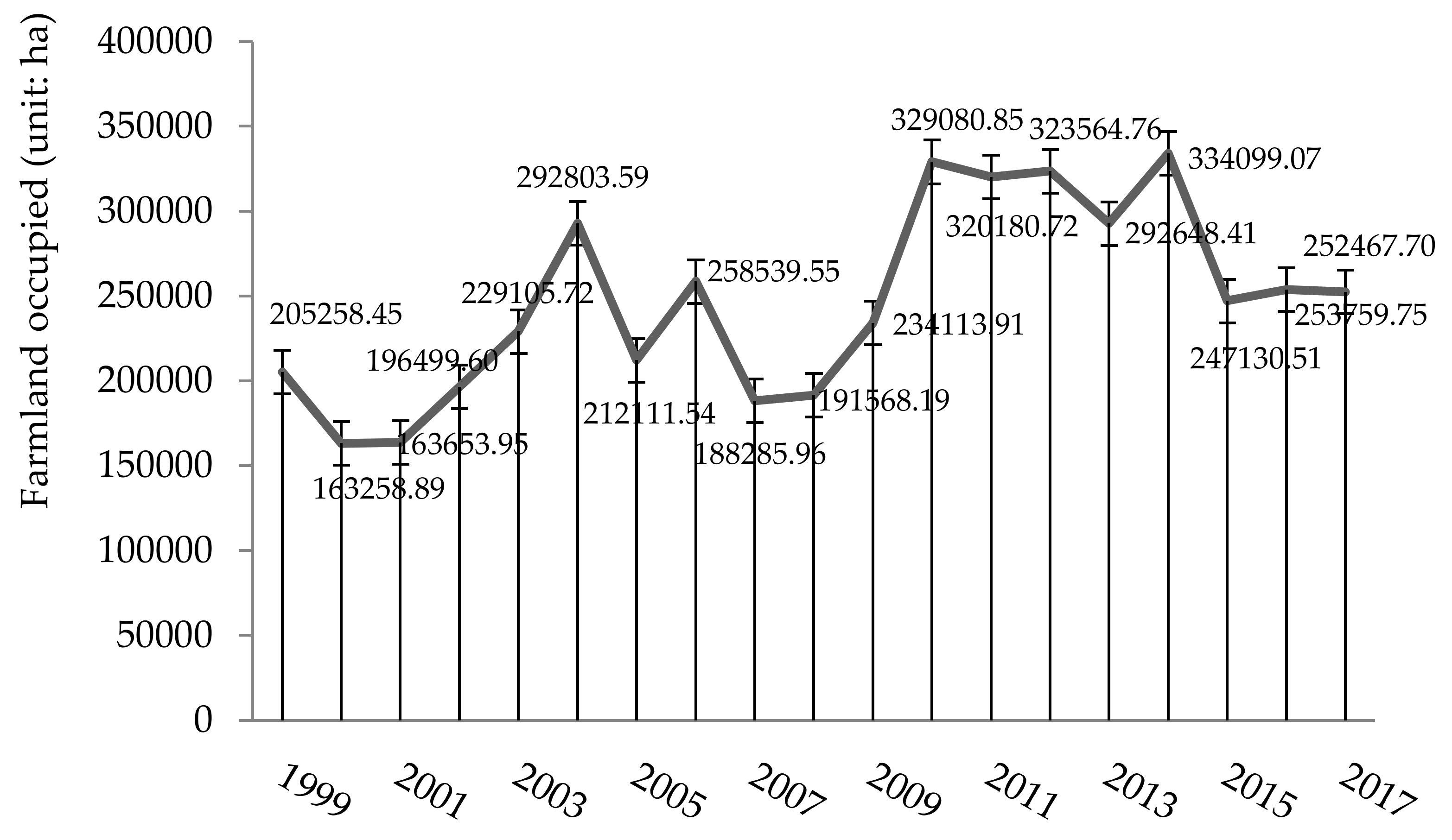
In recent decades, China has witnessed dramatic changes of land use/cover driven by rapid urbanization [38,39]. Nevertheless, urban development is dominated by urban sprawl and urban land use is inefficient. According to the findings in Jiao [40], most of the cities in China expanded rapidly and became less compact and more dispersed in recent years. Additionally, the rates at which the land use efficiency increased among cities were significantly low, with an average rate of 0.17% during 2007–2015 [41]. Under these circumstances, cities expand space mainly by occupying farmland, rather than by increasing the efficiency of land within the city. According to the latest China Land and Resources Statistical Yearbook, around 4.69 million ha of farmland has been occupied during 1999–2017 due to the significant demand of urban land for economic growth in China (Figure 1) [10]. There is clearly an urgent need to improve the urban land efficiency and to slow down the farmland loss in China.

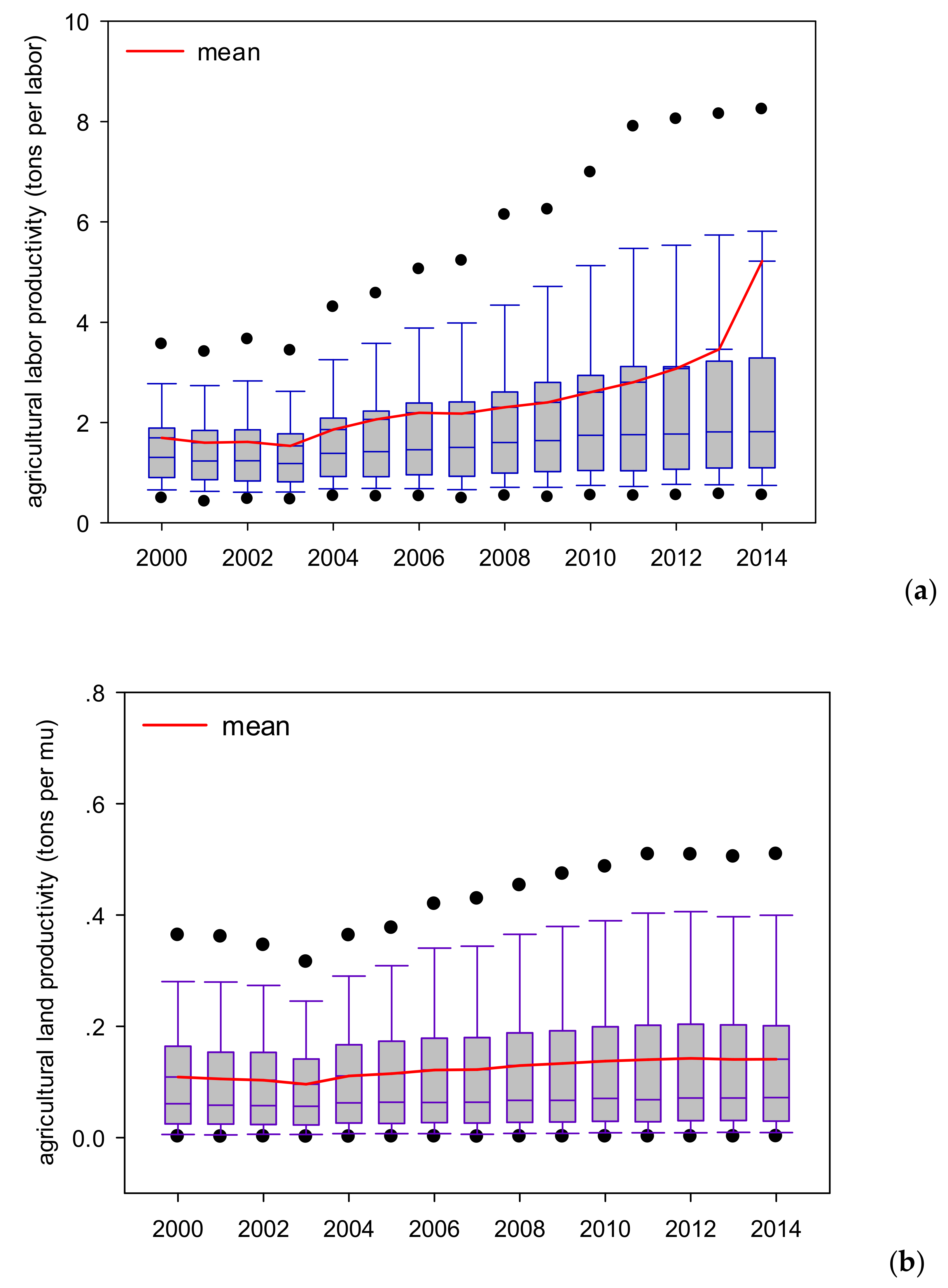
Before conducting an empirical analysis, we further utilized statistical data to perform a simple description and analysis to reveal some stylized facts about China’s agricultural productivity. Figure 2a shows the variation in agricultural labor productivity in China from 2000 to 2014, while Figure 2b shows the variation in agricultural land productivity in China from 2000 to 2014. In Figure 2a, Chinese agricultural labor productivity shows an obvious upward trend, while in Figure 2b, the upward trend of Chinese agricultural land productivity is not obvious. Generally, the technical level of labor has been improving significantly in the process of agricultural production in China; however, the single factor productivity of land does not improve significantly.

The period of 2000–2014 was the stage of a rapid upgrading of China’s technological level, and the production technology of agriculture and industry improved greatly (the industrial real added value increased by 311% and the agriculture real added value increased by 75%3). Why did agricultural land productivity not increase significantly during this period? An important reason may be that the decline of farmland quality partly offsets the improvements in farmland use technology, and among others, the RCBF policy may be one reason for the decline in farmland quality [17,25]. With the rapid urbanization in China, a large amount of high-quality farmland, especially paddy fields, is occupied [5,42]. As a result, the sloped lands, wastelands and dry farmlands are supplemented according to the RCBF policy, which is likely to reduce farmland quality. As one of the Chinese national development strategies, urbanization in China will be further promoted in the future [43]. Given that China’s high-quality farmland is limited, how to ensure that the quality of farmland will not decline during the implementation of the RCBF policy should be a key consideration of authorities.

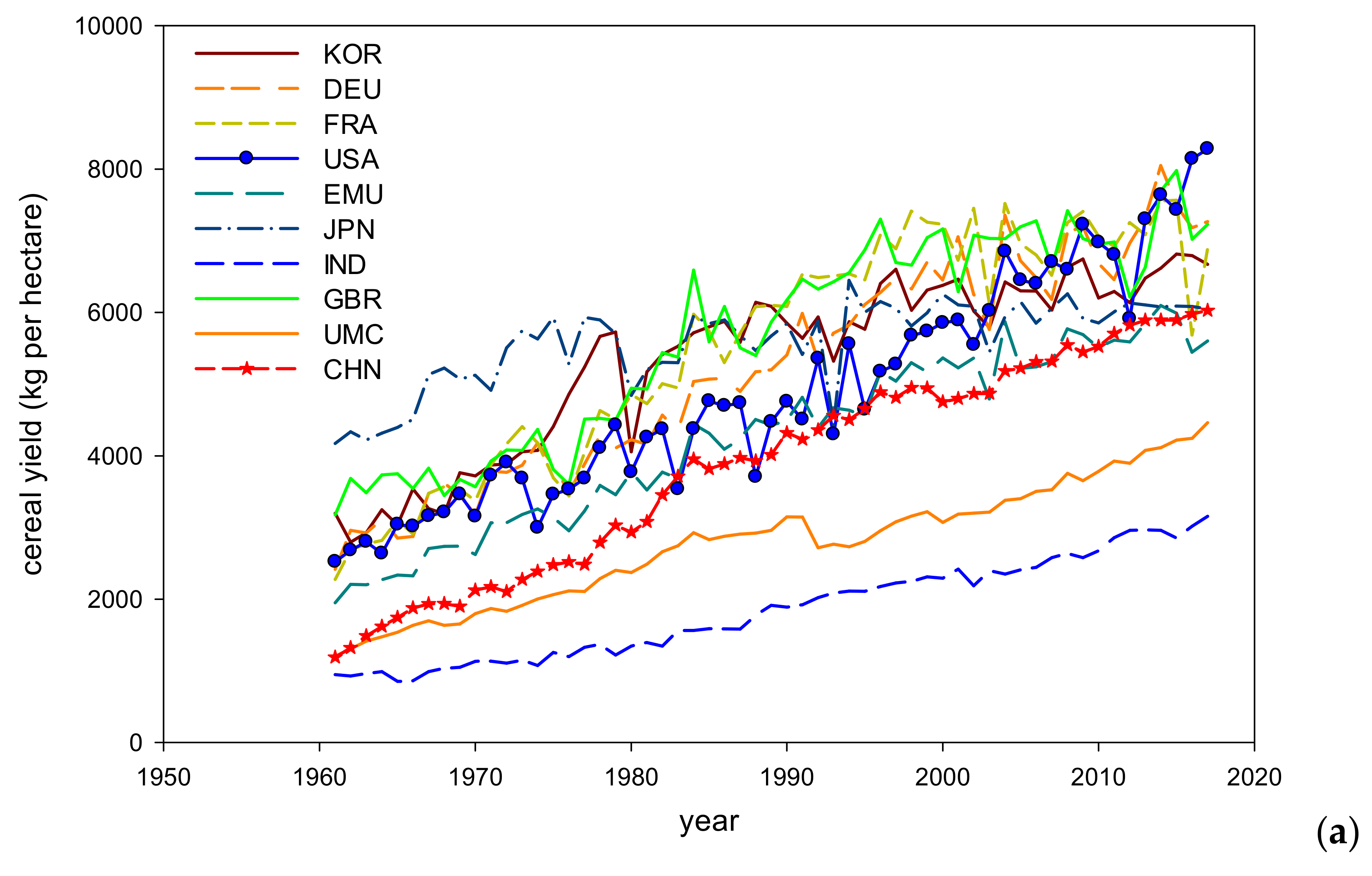
According to Figure 2a,b, we preliminarily consider that urbanization is an important reason for the slow increase in agricultural land productivity in China. To further confirm this judgment, we made an international comparison. Figure 3a shows that the trend of the cereal yield per unit land in China during 1961–2017 is basically the same as that in the developed countries. However, in the 1980s and 1990s, Chinese farmland productivity increased rapidly, which may have been due to the large-scale promotion of hybrid rice. After 2010, the increase in farmland productivity in China became relatively flat. An underlying reason for this result may be that after 2010, urban expansion occupied a large amount of farmland, and a large amount of high-quality land, such as paddy fields, was replaced by low-quality land—little remaining high-quality land could be used for supplementation after 2010, even consuming money and time for land consolidation—leading to a decline in the average land quality.

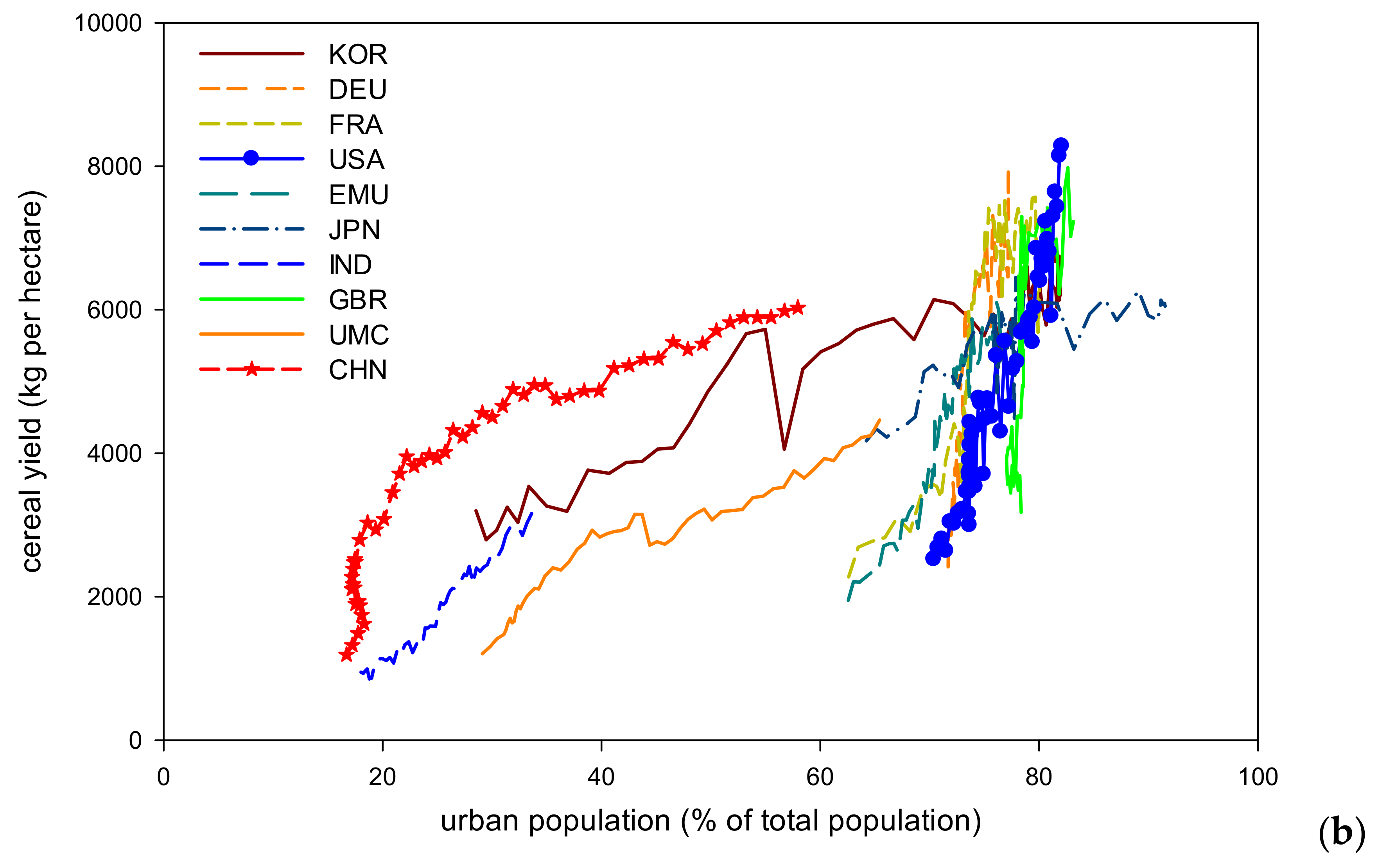
To illustrate the relationship between farmland productivity and urbanization more intuitively, we drew Figure 3b. Figure 3b shows that farmland productivity increases with urbanization, which is due to the considerable improvement of industrialization and the technology level accompanied by urbanization. Nonetheless, compared with the United States, the United Kingdom, Germany, Japan, the European Union and other major countries and regions, the level of farmland productivity in China has increased slowly with urbanization, especially when the urbanization rate exceeded 30% (i.e., after 1994). One reason for this result may be that the Chinese urbanization rate is relatively faster and the rate of farmland productivity improvement fails to keep up, because agricultural productivity grows slowly under the smallholder operation mode of the household contract responsibility system [44]. Another possible reason is that urbanization under the RCBF policy has led to a decline in farmland quality in China due to the “superior occupation and inferior compensation” and “paddy field occupation and dry land compensation” as discussed in paragraph 4 in the Introduction section [15,17,25,27,28]. In principle, the diffusion of farmland use technology is relatively easy; thus, China should have a backward advantage in terms of farmland productivity, and through the use of advanced agricultural machinery as well as pesticides and planting technology, China should be able to achieve a significant improvement in their farmland use efficiency in the short term. However, China’s farmland productivity level has not only been lower than that of other major countries for a long time, but has also had a relatively slow growth trend in recent years. If this trend is not caused by farmland use technology, then it must be related to the quality of farmland.

In addition, we can reveal the phenomenon that urbanization in China may reduce farmland productivity by comparing the outputs of different farm products per unit land. According to Chinese planting habits and natural conditions, the farmland occupied in the process of urban expansion is mainly used to plant cereals and rapeseed and is seldom used to plant cotton, which is planted mainly in exurban areas. From 1992 to 1999, the average annual increase rates of cereals and rapeseed outputs per hectare were 2.07% and 2.80%, respectively, and the average annual increase rate of cotton output per hectare was 2.88%, with no significant differences among the three. However, from 2011 to 2017, the average annual increase rates of cereals and rapeseed outputs per hectare were 1.43% and 1.92%, respectively, while the average annual increase rate of cotton output per hectare was 4.30%, which was 3.00 times that of cereals and 2.24 times that of rapeseed4. Why did the cotton output per hectare increase considerably from 2011 to 2017, while that of cereals and rapeseed increased slowly? A possible reason is that the exurban farmland planted with cotton was less affected by urbanization, while the quality of urban and suburban farmland planted with cereals and rapeseed was likely to decline due to the land replacement caused by rapid urbanization, given the previously mentioned consequences of the RCBF policy [27,45]. Taking Zhejiang Province as an example, the major large-scale infrastructure projects in Zhejiang are concentrated in Hangzhou–Jiaxing–Huzhou–Shaoxing (HJHS) plain, where the quality of cultivated land is high (i.e., grade 2–6). However, the corresponding compensated land are concentrated in Jinhua–Quzhou basin and Wenzhou–Taizhou coastal area, where the cultivated land quality grade is relatively low, ranging from grade 8 to 12 (emphasized by Peihua Song, an officer in Zhejiang land consolidation center [46]). These occupied lands in the HJHS plain are mainly planted with cereals and rapeseed, thus the quality of cereals and rapeseed planting land tends to decline after being replaced. In contrast, the land planted with cotton is rarely replaced, so the impact of the RCBF policy on the quality of cotton planting land is relatively small.

According to the above stylized facts, we suspect that urbanization in China might reduce farmland productivity, although this suspicion, based solely on simple statistical descriptions, lacks necessary control variables and a rigorous econometric analysis. To more accurately examine the impact of urbanization on agricultural land productivity in China, we propose a new development of the SFA method and utilize it to carry out an empirical analysis with Chinese county-level data.

3. Research Method: SFA with Endogeneity and Heterogeneity

SFA is an increasingly popular methodology used for performance evaluation and performance determinants research. Consider a stochastic frontier model with a one-sided inefficiency $u$, and suppose that the scale of $u$ depends on some variables $z$. The “one-step” SFA model specifies both the stochastic frontier and the way in which $u$ depends on $z$, and can be estimated in a single step. This is in contrast to a “two-step” procedure, where the first step is to estimate a standard stochastic frontier model or data envelopment analysis (DEA) model, and the second step is to estimate the relationship between the estimated $u$ and $z$ (e.g., Marschall and Flessa [47]; Chan et al. [48]). Wang and Schmidt [49] explained theoretically why two-step SFA procedures are biased, while Simar and Wilson [50,51], Cazals et al. [52], and Simar et al. [53] explained theoretically why two-step DEA procedures are biased. Based on these researches, this study considers the single-step SFA better, nonetheless, a standard SFA model cannot deal with the endogeneity issue of performance-influencing factors. Therefore, this study proposes an improved version of the single-step SFA method with endogeneity and heterogeneity.

Consider the following production-type stochastic frontier model with endogenous explanatory variables and a heterogeneous inefficiency distribution:

$$y_{it}=x_{1,it}^{\prime }\beta +v_{it}-u_{it},$$

(1)

where $y_{it}$ is output and $x_{1,it}$ is input vector. Following the literature, the disturbance term $v_{it}$ is i.i.d. $N\left(0,{\sigma }_v^2\right)$. The inefficiency $u_{it}$ is truncated and normal, whose expectations are determined by variables $x_{2,it}$, specifically,

$$u_{it}~N^{+}\left[x_{2,it}^{\prime }{\phi }_u,{\sigma }_u^2\right],$$

(2)

which implies the heterogeneity of the $u_{it}$ distribution. Note that $x_{1,it}$ and $x_{2,it}$ may overlap and there may exist endogenous variables in $x_{1,it}$ and $x_{2,it}$. The main purpose of this study is to identify the coefficient vector ${\phi }_u$.

Assume the endogenous variables in $x_{1,it}$ and $x_{2,it}$ satisfy:

$$\underset{p\times 1}{\underbrace{x_{it}}}=\underset{p\times pq}{\underbrace{Z_{it}}}\underset{pq\times 1}{\underbrace{\delta }}+\underset{p\times 1}{\underbrace{{\epsilon }_{it}}},$$

(3)

where $Z_{it}=I_p\otimes z_{it}^{\prime }$, and $z_{it}$ is a $q\times 1$ vector of all exogenous variables (i.e., instrumental variables). The variance–covariance matrix of ${\epsilon }_{it}$ is denoted by $\Omega$. Without a loss of generality,

$$\left[\begin{array}{c}{\tilde{\epsilon }}_{it}\\ v_{it}\end{array}\right]\equiv \left[\begin{array}{c}{\Omega }^{-1/2}{\epsilon }_{it}\\ v_{it}\end{array}\right]~\mathrm{N}\left(\left[\begin{array}{c}0\\ 0\end{array}\right],\left[\begin{array}{cc}{I}_p& {\sigma }_v\rho \\ {\sigma }_v{\rho }^{\prime }& {\sigma }_v^2\end{array}\right]\right)$$

(4)

where $\rho$ is the $p\times 1$ vector representing the correlation coefficients between ${\tilde{\epsilon }}_{it}$ and $v_{it}$. The correlation between ${\tilde{\epsilon }}_{it}$ and $v_{it}$ invalidates the conventional estimation of SFA, which requires $v_{it}$ and $u_{it}$ (and thus ${\tilde{\epsilon }}_{it}$) are independent.

By a Cholesky decomposition of the variance–covariance matrix of ${\left({\tilde{\epsilon }}_{it}^{\prime }, v_{it}\right)}^{\prime }$, we can represent ${\left({\tilde{\epsilon }}_{it}^{\prime },v_{it}\right)}^{\prime }$ as follows:

$$\left[\begin{array}{c}{\tilde{\epsilon }}_{it}\\ v_{it}\end{array}\right]=\left[\begin{array}{cc}{I}_p& 0\\ {\sigma }_v{\rho }^{\prime }& {\sigma }_v\sqrt{1-{\rho }^{\prime }\rho }\end{array}\right]\left[\begin{array}{c}{\tilde{\epsilon }}_{it}\\ {\tilde{w}}_{it}\end{array}\right],$$

(5)

where ${\sigma }_v\sqrt{1-{\rho }^{\prime }\rho }$ is scalar, and ${\tilde{\epsilon }}_{it}$ and ${\tilde{w}}_{it}~N\left(0,1\right)$ are independent. By this decomposition, $v_{it}={\sigma }_v{\rho }^{\prime }{\tilde{\epsilon }}_{it}+{\sigma }_v\sqrt{1-{\rho }^{\prime }\rho }{\tilde{w}}_{it}$. Therefore, Equation (1) can be represented as:

$$y_{it}=x_{1,it}^{\prime }\beta +{\sigma }_v{\rho }^{\prime }{\tilde{\epsilon }}_{it}+{\sigma }_v\sqrt{1-{\rho }^{\prime }\rho }{\tilde{w}}_{it}-u_{it}$$

(6)

Let $w_{it}\equiv {\sigma }_v\sqrt{1-{\rho }^{\prime }\rho }{\tilde{w}}_{it}$, then its standard deviation is ${\sigma }_w={\sigma }_v\sqrt{1-{\rho }^{\prime }\rho }$ and therefore,

$$y_{it}=x_{1,it}^{\prime }\beta +{\sigma }_v{\rho }^{\prime }{\tilde{\epsilon }}_{it}+w_{it}-u_{it}$$

(7)

Substituting ${\tilde{\epsilon }}_{it}={\Omega }^{-1/2}{\epsilon }_{it}$ into Equation (7) yields:

$$y_{it}=x_{1,it}^{\prime }\beta +{\eta }^{\prime }\left(x_{it}-Z_{it}\delta \right)+e_{it},$$

(8)

where $\eta \equiv {\sigma }_w{\Omega }^{-1/2}\rho /\sqrt{1-{\rho }^{\prime }\rho }$ and $e_{it}\equiv w_{it}-u_{it}$.

In Equation (8), $w_{it}$ and $u_{it}$ are conditionally independent from the regressors given $x_{it}$ and $z_{it}$ [54,55], and $u_{it}~N^{+}\left[x_{2,it}^{\prime }{\phi }_u,{\sigma }_u^2\right]$, $w_{it}~N\left[0,{\sigma }_W^2\right]$. According to Equation (8), endogeneity can be viewed as an omitted variable problem. Now, we can use the maximum likelihood method to estimate Equation (8). Denote $T_i$ as the number of time periods for panel $i$ (for a balanced panel $T_i=T$); then, with the conditional probability formula, the log-likelihood of panel $i$ is given by:

$$\ln L_i=\ln L_{i,y\left|x\right.}+\ln L_{x,i},$$

(9)

where

$$\ln L_{i,y\left|x\right.}=\sum _{t=1}^{t=T_i}\left\{-\frac{1}{2}\ln \left({\sigma }_w^2+{\sigma }_u^2\right)+\ln \varphi \left(\frac{{\mu }_{it}+e_{it}}{\sqrt{{\sigma }_w^2+{\sigma }_u^2}}\right)+\ln \mathsf{\Phi }\left(\frac{{\mu }_{*it}}{{\sigma }_{*it}}\right)-\ln \mathsf{\Phi }\left(\frac{{\mu }_{it}}{{\sigma }_u}\right)\right\},$$

$$\ln L_{x,i}=\sum _{t=1}^{t=T_i}\left\{\frac{-p\ln \left(2\pi \right)-\ln \left|\Omega \right|-{\epsilon }_{it}^{\prime }{\Omega }^{-1}{\epsilon }_{it}}{2}\right\},$$

$${\mu }_{it}=x_{2,it}^{\prime }{\phi }_u,$$

$$e_{it}=y_{it}-x_{1,it}^{\prime }\beta -{\eta }^{\prime }\left(x_{it}-Z_{it}\delta \right),$$

$${\epsilon }_{it}=x_{it}-Z_{it}\delta ,$$

$${\mu }_{*it}\equiv \frac{{\sigma }_w^2{\mu }_{it}-{\sigma }_u^2{e}_{it}}{{\sigma }_w^2+{\sigma }_u^2},$$

$${\sigma }_{*it}^2\equiv \frac{{\sigma }_w^2{\sigma }_u^2}{{\sigma }_w^2+{\sigma }_u^2},$$

and $\varphi \left(·\right)$ and $\mathsf{\Phi }\left(·\right)$ denote the standard normal probability density function and cumulative distribution function, respectively. As mentioned above, the main purpose of this study is to identify the coefficient vector ${\phi }_u$, which includes the influencing coefficient of urbanization on farmland productivity.

Furthermore, the efficiency (productivity) can be predicted by:5

$$\mathrm{E}\left[\exp \left(-u_{it}\right)\left|e_{it}\right.\right]=\exp \left(-{\mu }_{*it}+\frac{1}{2}{\sigma }_{*it}^2\right)\frac{\mathsf{\Phi }\left(\frac{{\mu }_{*it}}{{\sigma }_{*it}}-{\sigma }_{*it}\right)}{\mathsf{\Phi }\left(\frac{{\mu }_{*it}}{{\sigma }_{*it}}\right)}.$$

(10)

Following the study of Murphy and Topel [56], Karakaplan and Kutlu [55] proposed a two-step maximum likelihood estimation to simplify computation. In the first stage, $\ln L_{x,i}$ is maximized with respect to the relevant parameters $\delta$; in the second stage, which is conditional on the parameters estimated in the first stage, $\ln L_{i, y\left|x\right.}$ is maximized. Furthermore, the well-known fixed/random effects can be considered when estimating Equation (8), that is,

$$y_{it}=x_{1,it}^{\prime }\beta +{\eta }^{\prime }\left(x_{it}-Z_{it}\delta \right)+a_i+e_{it},$$

(11)

where the unobserved heterogeneity $a_i$ is distributed as $N\left(0,{\theta }^2\right)$, and $E\left(a_i\left|x_{1,it},x_{it}-Z_{it}\delta \right.\right)=0$. Belotti et al. [57] provided an unbiased method to estimate the parameter $\theta$.

In this study, we research the impact of urbanization on farmland productivity and use the grain yield as the output (i.e.,$y_{it}=\ln \left(Grai{n}_{it}\right)$); the agricultural labor ($Agrilabo{r}_{it}$), farmland area ($Agrilan{d}_{it}$), fertilizer ($Fert{i}_{it}$) and machinery ($Mach{i}_{it}$) as the inputs (i.e., $x_{1,\mathrm{it}}^{\prime }=\left(1,\ln Agrilabo{r}_{it},\ln Agrilan{d}_{it},\ln Fert{i}_{it},\ln Mach{i}_{it}\right)$); the urbanization rate ($Urba{n}_{it}$), farmland area per household ($Land\_ho{u}_{it}$), industrialization level ($gdp\_{21}_{it}$), and per capita net income of farmers ($Agri\_incom{e}_{it}$) as the factors affecting farmland productivity (i.e., $x_{2,it}^{\prime }=\left(1,\ln Urba{n}_{it},\ln Land\_ho{u}_{it},\ln gdp\_{21}_{it},\ln Agri\_incom{e}_{it}\right)$). The data sources and endogeneity of the variables will be described in Section 4.

4. Data Sources and Empirical Results

4.1. Data Sources

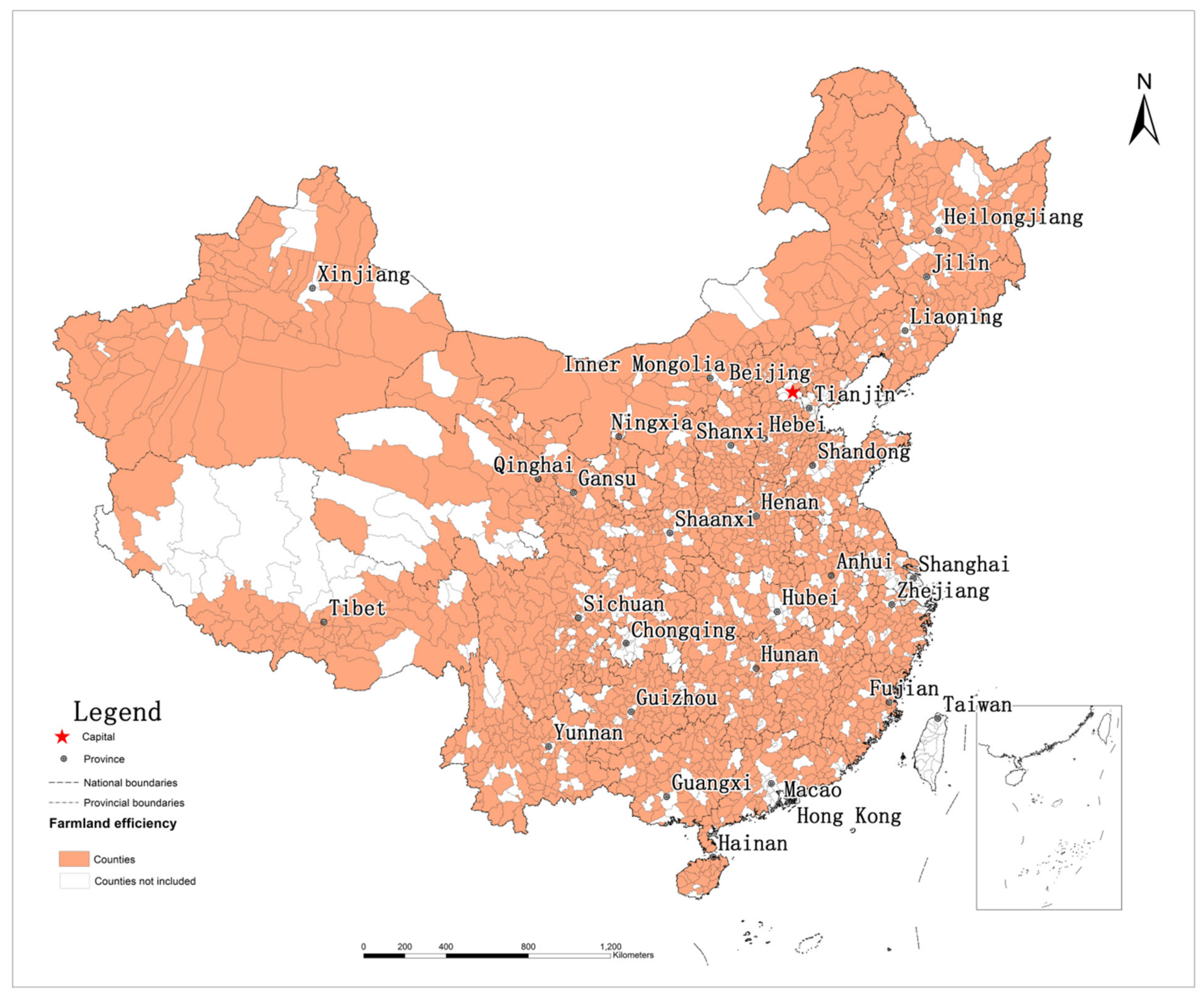
An empirical analysis based on county-level panel data can better uncover the changes in agricultural land productivity driven by urbanization and have meaningful policy implications. In this study, counties with the following three characteristics are excluded: (1) the administrative jurisdiction area changes during the time interval; (2) there is very little agricultural land within the county; (3) a large proportion of indicators are missing (for five consecutive years or more). Finally, 1961 counties were selected as the panel sections6 (the counties included in our study are shown in Appendix A Figure A1). Based on the time course of rural laborers’ off-farm employment in China and the availability of county-level data, the time series of this study covers the period from 2000 to 20147. The data are mainly drawn from the China Statistical Yearbook (County-level, 2001–2015) and the bulletins issued yearly by the 1961 county governments. County-level agricultural land data were obtained by an application from the Ministry of Natural Resources. The descriptive statistics of the variables are presented in

Table 1. Variable definitions and descriptive statistics.

Variable		Description	Mean	Std. Dev.	Unit	Time Period	Obs
Variables to calculate agricultural land use efficiency	Agriland	Agricultural land for planting, forestry, animal husbandry and fishery	26.5318	36.0115	10,000 ha	2001–2014, yearly	29,415
	Agrilabor	Rural laborers occupied in planting, forestry, animal husbandry and fishery	12.5207	9.7501	10,000 person	2000–2014, yearly	29,415
	Machi	Total power of agricultural machinery	32.7981	35.0660	10,000 kw	2000–2014, yearly	29,415
	Ferti	Consumption of chemical fertilizers	2.1152	2.2128	10,000 tons	2000–2014, yearly	29,415
	Grain	Output of grain	24.4166	27.3292	10,000 tons	2000–2014, yearly	29,415
Independent variables	Urban_1	Proportion of rural laborers engaged in off-farm employment	0.3515	0.1722	-	2000–2014, yearly	29,415
	Urban_2	Ratio of built-up area to administrative area	0.0091	0.0142	-	2004–2011, yearly	14,609
	gdp_21	Ratio of the output values of secondary and primary industries	3.2529	7.9313	-	2000–2014, yearly	29,415
	Agri_income	Net income of rural households per capita of a county	4655	3529	yuan per capita	2000–2014, yearly	29,415
	Land_hou	Cultivated land area per household	1.1972	8.7919	ha per household	2000–2014, yearly	29,415

.

To control the potential impact of price, the grain yield (Grain), rather than the total agricultural product value, was selected as the output variable. The grain yield includes the total amount of grain, beans, and tubers in the county in one year. The yield of various crops was converted according to the standard grain approach when summarizing the statistical data.

The input variables were selected according to the classification of production factors by production function. Specifically, agricultural laborers (Agrilabor) represent the labor force over the age of 16 among the rural population who actually participate in agricultural production and operation activities. Agricultural land (Agriland) is the land input for agricultural production that comprehensively controls the differences in multiple cropping indices across counties and the land use types of different crops by using the total and direct area of farmland. The consumption of chemical fertilizers (Ferti) and the total power of agricultural machinery (Machi) denote the efforts of Chinese peasants using capital and technology to farm.

Influencing factors on farmland efficiency include the (1) urbanization rate measured by two types of urbanization, which are the demographic urbanization measured by the proportion of rural laborers engaged in off-farm employment (Urban_1) and the land urbanization measured by the ratio of the built-up area to the administrative area (Urban_2); (2) Land_hou, the arable land area per household, which controls the effect of the rural land use scale on the agricultural efficiency; (3) gdp_21, the ratio of the output values of the secondary industry to the primary industry, which reflects the industrialization degree of a county; (4) Agri_income, the net income of rural households per capita, controlling the influence of capital constraints on efficiency.

4.2. Regression Results

This study uses time-varying SFA models for regression, and the results are shown in

Table 2. The results of empirical test (2000–2014).

	Model 1		Model 2		Model 3		Model 4		Model 5		Model 6
	Urbanization Rate (Urban) is Measure by Urban_1						Urbanization Rate (Urban) is Measure by Urban_2
	Coef.	Std. Err.	Coef.	Std. Err.	Coef.	Std. Err.	Coef.	Std. Err.	Coef.	Std. Err.	Coef.	Std. Err.
Frontier
Constant	9.377 ***	0.097	10.449 ***	0.104	6.045 ***	0.075	5.910 ***	0.105	7.144 ***	0.068	5.695 ***	0.108
$\ln Agrilabor$	0.061 ***	0.005	0.086 ***	0.005	0.280 ***	0.005	0.225 ***	0.007	0.073 ***	0.004	0.223 ***	0.007
$\ln Agriland$	0.105 ***	0.005	0.016 ***	0.005	0.140 ***	0.004	0.183 ***	0.005	0.246 ***	0.004	0.200 ***	0.006
$\ln Ferti$	0.218 ***	0.005	0.226 ***	0.004	0.429 ***	0.004	0.433 ***	0.006	0.338 ***	0.004	0.437 ***	0.006
$\ln Machi$	0.068 ***	0.003	0.070 ***	0.003	0.285 ***	0.004	0.326 ***	0.006	0.121 ***	0.004	0.319 ***	0.006
Inefficiency
Constant	9.617 ***	0.988	–2.610	2.407	–35.943 ***	3.184	–76.725 ***	11.983	–80.086 **	30.959	–103.829 ***	16.346
$\ln Urban$	–1.222 ***	0.114	–16.140 ***	2.163	–8.264 ***	0.681	–3.159 ***	0.446	–7.845 **	3.648	–8.923 ***	1.553
${\left(\ln Urban\right)}^2$			–2.858 ***	0.400	–1.216 ***	0.111			–0.069	0.137	–0.392 ***	0.081
$\ln Land\_hou$	2.556 ***	0.138	3.752 ***	0.362	–1.684 ***	0.119	–1.987 ***	0.290	6.836 ***	1.875	–2.032 ***	0.280
$\ln gdp\_21$	0.934 ***	0.076	2.102 ***	0.245	0.709 ***	0.077	0.221	0.141	1.975 ***	0.709	0.348 **	0.147
$\ln Agri\_income$	–2.440 ***	0.184	–4.168 ***	0.502	2.507 ***	0.234	5.563 ***	0.903	–0.957	0.913	6.385 ***	1.008
Standard deviations
$\theta$	1.457 ***	0.012	1.304 ***	0.009					0.906 ***	0.005
${\sigma }_u$	1.414 ***	0.053	2.167 ***	0.132	1.550 ***	0.073	2.100 ***	0.176	3.011 ***	0.491	2.146 ***	0.181
${\sigma }_v$	0.090 ***	0.001	0.089 ***	0.001	0.398 ***	0.003	0.394 ***	0.004	0.030 ***	0.002	0.395 ***	0.004
$\lambda$	15.776 ***	0.053	24.324 ***	0.132	3.890 ***	0.074	5.335 ***	0.176	99.308 ***	0.491	5.427 ***	0.181

Notes: ** Significant at 5%; *** Significant at 1%.

. In Table 2, Models 1–3 use the rural labor transfer rate to measure the urbanization rate, while Models 4–6 use the proportion of the built-up area to measure the urbanization rate. Models 1, 2 and 5 use the true random effects model proposed by Greene [59] and Belotti et al. [57], while Models 3, 4 and 6 use the maximum likelihood random effects time-varying inefficiency effects model proposed by Battese and Coelli [60] to regress the SFA model presented in Section 3. The endogeneity of the urbanization rate will be addressed with our empirical method later.

According to Models 1 and 4, urbanization decreases the inefficiency of farmland use and thus increases the farmland use efficiency. Therefore, overall, the technology improvement effect caused by urbanization is stronger than the land-quality-decrease effect caused by the RCBF policy or the other abovementioned reasons. According to Models 2, 3, 5, and 6, when considering the quadratic term of the urbanization rate, there is an inverted U-shaped relationship; accordingly, there is a U-shaped relationship between the farmland use efficiency and urbanization rate. This U-shaped relationship indicates that only when the urbanization rate is relatively low would urbanization decrease the farmland use efficiency, that is, when the undesirable effect of urbanization mentioned in Section 1 is dominant. We consider that the decrease is mainly due to a large amount of superior occupation and inferior compensation, which is a direct consequence of the RCBF policy. However, when the urbanization rate is relatively high, the technical progress accompanied by factor agglomeration is obvious, and few superior lands remain; thus, the land-quality-decrease effect caused by the RCBF policy is offset.

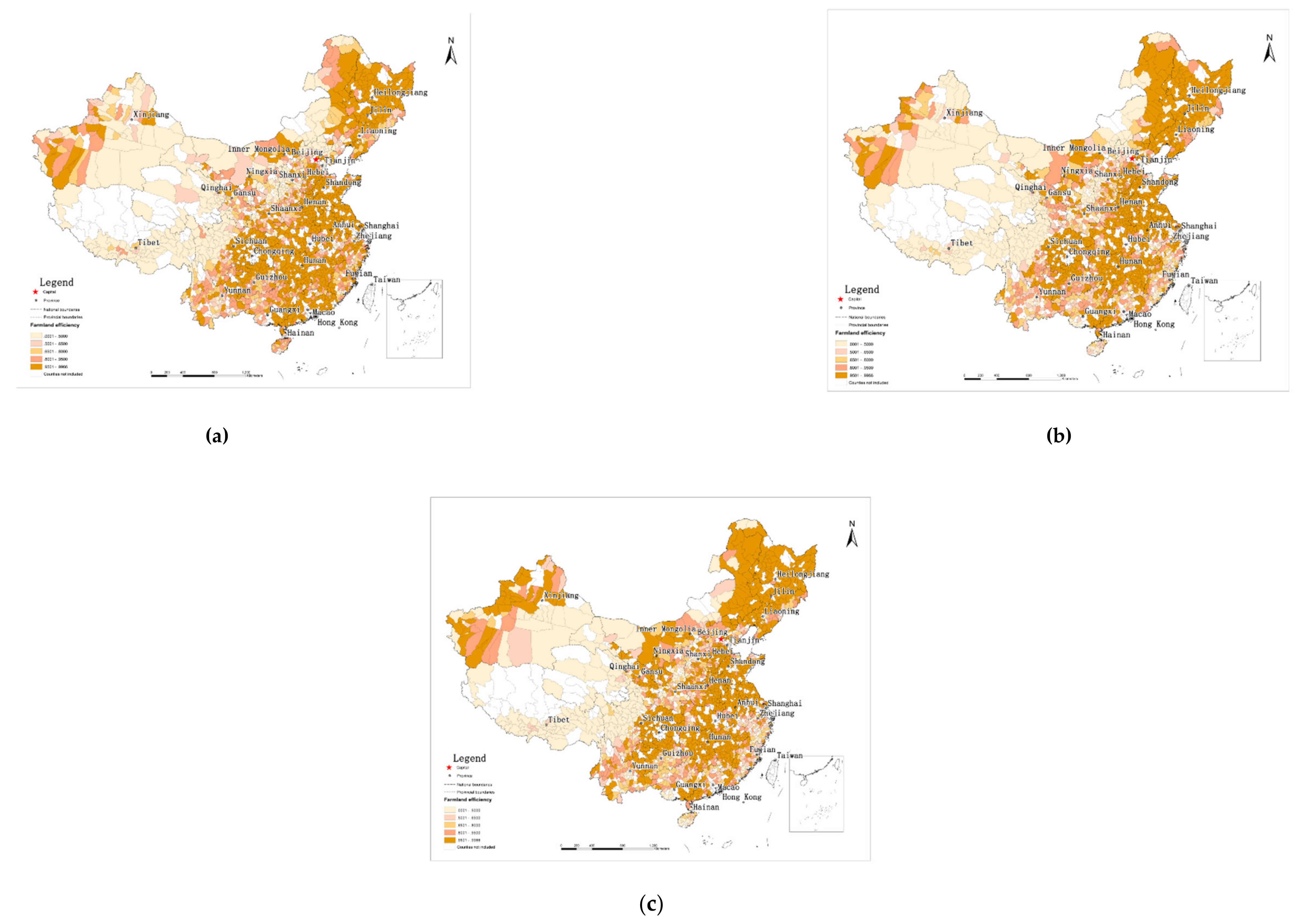
Comparing these models, we consider the regression method proposed by Greene [59] and Belotti et al. [57] to be better, although this method often does not converge. Meanwhile, the urbanization rate measured by the rural labor transfer rate is better; otherwise, if we use the proportion of built-up area to measure the urbanization rate, 14,806 samples are missing because of no data, and a serious data error exists. In addition, in China, the built-up area is often planned by local governments and remains unchanged for many years. Therefore, we focus on the results of Models 2 and 3. In Model 2, the inflection point of the (inverted) U-shaped relationship is equal to $-16.14/\left(2\times 2.858\right)=-2.824$. In the sample data, the real log of the urbanization rate is from $-7.0010$ to $-0.0004$, with an average value of $-1.2073$; thus, only a few counties experience the inflection point. The spatiotemporal change in farmland productivity across counties in 2000, 2007, 2014, measured based on Model 2, is shown in Appendix A Figure A2a–c.

The farmland use efficiency also usually affects the urbanization rate because a higher farmland use efficiency liberates labor from agricultural production, and thus, more migrant workers enter cities. Taking into account the endogeneity of the urbanization rate, we carry out a robustness test for the results in Table 2. We use the lag of the urbanization rate ($L\_\ln Urban$) and the added-value ratio of the secondary and primary industries ($\ln gdp\_21$) as exogenous instrumental variables of the urbanization rate. With the empirical method presented in Section 3, the SFA results with endogeneity and heterogeneity are shown in

Table 3. The results of empirical test after considering endogeneity (2000–2014).

	Model 7		Model 8		Model 9
	Coef.	Std. Err.	Coef.	Std. Err.	Coef.	Std. Err.
	Urban=Urban_1				Urban=Urban_2
Frontier
Constant	6.323 ***	0.078	6.086 ***	0.078	5.780 ***	0.116
$\ln Agrilabor$	0.265 ***	0.005	0.271 ***	0.005	0.205 ***	0.008
$\ln Agriland$	0.129 ***	0.004	0.141 ***	0.004	0.204 ***	0.006
$\ln Ferti$	0.431 ***	0.004	0.431 ***	0.004	0.437 ***	0.006
$\ln Machi$	0.305 ***	0.005	0.298 ***	0.005	0.340 ***	0.007
Inefficiency
Constant	–35.194 ***	3.990	–35.040 ***	3.175	–105.712 ***	18.144
$\ln Urban$	–3.487 ***	0.323	–8.341 ***	0.706	–9.158 ***	1.742
${\left(\ln Urban\right)}^2$			–1.279 ***	0.121	–0.401 ***	0.091
$\ln Land\_hou$	–1.822 ***	0.180	–1.634 ***	0.118	–1.990 ***	0.297
$\ln gdp\_21$	0.768 ***	0.114	0.663 ***	0.075	0.426 ***	0.163
$\ln Agri\_income$	2.504 ***	0.307	2.447 ***	0.234	6.428 ***	1.105
Standard deviations
${\sigma }_u$	1.855 ***	0.108	1.518 ***	0.074	2.193 ***	0.201
${\sigma }_v$	0.402 ***	0.003	0.400 ***	0.003	0.395 ***	0.004
$\lambda$	4.617 ***	0.108	3.795 ***	0.074	5.557 ***	0.201
Endogeneity test
$\eta$	–0.021	0.015	–0.034 **	0.014	–0.031 *	0.016

Notes: * Significant at 10%; ** Significant at 5%; *** Significant at 1%.

. To ensure the convergence of the maximum likelihood estimation, Models 7–9 use the method proposed by Battese and Coelli [60] to simplify the SFA.

In Table 3, the coefficients of the urbanization rate and its quadratic term are significantly negative, implying that the (inverted) U-shaped relationship still holds after taking into account the endogeneity of the urbanization rate. Thus, the land productivity-decrease effect caused by urbanization is fully offset by the technical progress effect accompanied by urbanization when the urbanization rate is relatively high. To illustrate the existence of the land productivity-decrease effect, we selected the sample with a log of urbanization rate lower than –2.824 to perform Modes 1 and 7 again, and then the coefficients of $\ln Urban$ become insignificantly positive8. In Table 3, the endogeneity tests show that the endogeneity of the urbanization rate should be taken into account when adding a quadratic term, although this does not affect the main conclusion of this study.

4.3. Robust Analysis: Total-Factor Farmland Use Efficiency

The total-factor productivity is the farmland use efficiency obtained by the SFA method, which involves the efficiencies with respect to all the factors, not only with respect to farmland. To address this issue, one could use the single-factor productivity—the grain yield per agricultural land—to measure the land use efficiency, which, however, does not control the interference of other inputs. Therefore, we utilize the directional distance function (DDF) method to obtain the total-factor farmland use efficiency (TFLE)9 and investigate the impact of urbanization on it as a robustness analysis.

A large number of studies have examined the properties of the DDF, such as Chambers et al. [62], Färe et al. [63], Feng and Serletis [64], and Atkinson and Tsionas [65]. For the production possibility set of the DDF (namely, ${\mathbb{T}}^{\mathrm{DDF}}$), if using all the data for all the decision-making units (DMUs) and periods to construct frontiers, then ${\mathbb{T}}^{\mathrm{DDF}}$ indicates a global benchmark technology [66,67]. If using the current and next-period data to construct frontiers, then ${\mathbb{T}}^{\mathrm{DDF}}$ indicates a biennial benchmark technology [68,69]. If using the current and previous data to construct frontiers, then ${\mathbb{T}}^{\mathrm{DDF}}$ indicates a sequential benchmark technology [70]; in most studies, such as Färe et al. [63] and Deng et al. [71], only contemporaneous data are used to construct the technology frontiers. To make the TFLE comparable, this study prefers to adopt the global benchmark technology, but the big data with 29,415 DMUs makes computation difficult; thus, this study uses 500 DMUs that have the highest grain yield per agricultural land to construct the technology frontiers, whose inputs and output are denoted by $\left(Agrilan{d}^F,Agrilabo{r}^F,Fert{i}^F,Mach{i}^F,Grai{n}^F\right)$.

Different from a conventional DDF, since we aim to compute the TFLE rather than total-factor efficiency, we use the following land-oriented DDF:

$$\overrightarrow{DDF}=\max \left\{\vartheta :\left(Agriland\left(1-\vartheta \right),Agrilabor,Ferti,Machi,Grain\right)\in {\mathbb{T}}^{\mathrm{DDF}}\right\},$$

(12)

$${\mathbb{T}}^{\mathrm{DDF}}=\left\{\left(Agriland,Agrilabor,Ferti,Machi,Grain\right)|\begin{array}{c}{\displaystyle \sum }_{i=1}^{500}{\zeta }_{i}Agrilan{d}_i^F\le Agriland\\ {\displaystyle \sum }_{i=1}^{500}{\zeta }_{i}Agrilabo{r}_i^F\le Agrilabor\\ {\displaystyle \sum }_{i=1}^{500}{\zeta }_{i}Fert{i}_i^F\le Ferti\\ {\displaystyle \sum }_{i=1}^{500}{\zeta }_{i}Mach{i}_i^F\le Machi\\ {\displaystyle \sum }_{i=1}^{500}{\zeta }_{i}Grai{n}_i^F\ge Grain\\ {\displaystyle \sum }_{i=1}^{500}{\zeta }_i=1;{\zeta }_i\ge 0\end{array}\right\},$$

where ${\zeta }_i$ ($i=1,\dots ,500$) are the intensity variables representing the weights that each selected DMU contributes to determining the corresponding technology frontier. Because the computed values of the DDF are a measure of inefficiency, the TFLE can therefore be obtained by $1-\overrightarrow{DDF}$ [67,72,73,74].

With the estimated TFLE, we carried out a robustness test, shown in

Table 4. Robustness tests (2000–2014).

	Model 10		Model 11		Model 12
	Fixed	Random	Fixed	Random	Fixed	Random
Constant	1.208 ***	1.263 ***	0.099 ***	0.107 ***	–0.137 ***	–0.124 ***
$\ln Urban$	0.155 ***	0.167 ***	0.009 ***	0.011 ***	0.032 ***	0.036 ***
${\left(\ln Urban\right)}^2$	0.025 ***	0.027 ***	0.002 ***	0.003 ***	0.006 ***	0.007 ***
$\ln Land\_hou$	0.072 ***	0.056 ***	0.003	–0.004 **	0.023 ***	0.012 ***
$\ln gdp\_21$	–0.029 ***	–0.028 ***	–0.002 ***	–0.002 ***	–0.006 ***	–0.006 ***
$\ln Agri\_income$	–0.034 ***	–0.040 ***	0.016 ***	0.015 ***	0.038 ***	0.036 ***

Notes: Fixed means fixed effect model; Random means random effect model; ** Significant at 5%; *** Significant at 1%.

, in which Model 10 uses the SFA efficiency obtained using Model 3 and Equation (10) to measure the farmland use efficiency, while Model 11 and Model 12 use the TFLE obtained using the DDF method and grain yield per agricultural land, respectively, to measure the farmland use efficiency. In the three models of Table 4, all the coefficients of $\ln Urban$ and its quadratic term are significantly positive, showing a U-shaped relationship between the farmland use efficiency and urbanization rate. Therefore, the aforementioned conclusion—only when the urbanization rate is relatively low would urbanization reduce the farmland use efficiency and when the urbanization rate is relatively high, the land productivity-decrease effect is offset by technical progress—is robust.

In Models 2 and 10, the inflection points of the U-shaped relationship are approximately $-2.8$ and $-3.1$, respectively, while they are $-2.3$, $-1.8$, $-2.7$, and $-2.6$ in Model 11_fixed effect, Model 11_random effect, Model 12_fixed effect, and Model 12_random effect, respectively. Therefore, the inflection point is higher when considering the TFLE or grain yield per agricultural land. A possible reason for this result is that the total-factor efficiency used in Models 2 and 10 includes the productivity of all factors; therefore, the land productivity-decrease effect is partly offset by the high productivity of other factors.

5. Conclusions and Policy Implications

The United Nations predicted that the global urban population will gain an additional 2.5 billion people by 2050 [75]. Urbanization has been an inevitable process in China and China’s urbanization and farmland protection has attracted attention from around the world [42,43]. Nonetheless, China’s arable land is very limited with respect to its large population. As a result, urbanization in China has to occupy a considerable amount of farmland to develop industry and commerce as well as residence. To avoid food security issues due to the requisition of farmland, the RCBF policy was initiated by the Chinese government at the end of the 1990s. As a result of this policy, a land productivity-decrease effect may occur because of a “superior occupation and inferior compensation”, such as “paddy field occupation and dry land compensation”. Meanwhile, farmland use efficiency may decline because of “urban or suburban occupation and rural compensation” and because urbanization promotes more migrant workers to enter cities, which leads to an older population, who are less productive, being left behind in the countryside, and people often become lazy after getting a large land-lost compensatory payment. In summary, this study considers that urbanization could produce two effects for farmland use efficiencies—a positive effect due to technical progress and economies of scale, as well as an undesirable effect because of decreases in land quality and a labor force that is less productive.

To illustrate this assumption, we first show some stylized facts and then carried out empirical tests with a new efficiency measurement method—SFA with endogeneity and heterogeneity. After a great deal of effort to process the data, we selected 29,415 samples at the Chinese county-level from 2000–2014 for an empirical analysis. The results show that there is a U-shaped relationship between the farmland use efficiency and urbanization rate, indicating that only when the urbanization rate is relatively low would urbanization decrease the farmland use efficiency; in contrast, when the urbanization rate is relatively high, the technical progress accompanied by urbanization is obvious, and thus, the undesirable effect is offset. The U-shaped relationship results from the positive and undesirable effects of urbanization, but the latter has long been neglected by researchers. Taking into account the endogeneity of the urbanization rate and total-factor farmland use efficiency, the result is robust.

Revealing the positive and undesirable effects of urbanization on the farmland use efficiency is crucial for policy making in the sustainable management and conversation of farmland resources. Based on the above findings, the following recommendations are made. First, a complete RCBF policy system has not yet been established and maintaining a quantity–quality–ecology–productivity balance when occupying farmland is necessary. Without taking the productivity into account, the dynamical equilibrium of the total cultivated land was difficult to guarantee [76]. For a given area, if superior land is limited, then more inferior land is needed to compensate for one unit of superior land. In recent years, to encourage the rural population to agglomerate, the government has provided a large number of cash subsidies to relocated farmers, but the premise of the subsidy is that the former homestead must be turned into farmland. This policy has a complementary effect on the RCBF policy; however, if the farmers move far away, the farmland is often inefficiently used and even abandoned due to the changes driven by the increase in commuting costs. Changes in the allocation of farmland resources have brought about many problems and challenges for rural development [77]. Therefore, in terms of the effective use of agricultural land, China should encourage “local urbanization” (i.e., people from rural areas nearby gaining urban residency).

Second, the positive effect of urbanization is amplified by encouraging technology diffusion and mechanized farming. For example, modern agriculture should be developed, such as green agriculture, sightseeing agriculture, characteristic agriculture, experience agriculture and online–offline agriculture. The premise of developing modern agriculture is the scale operation of land; thus, it is also an urgent task to enable a way of land transition that is more flexible. Properly coordinating the relationship between farmland transition and urban–rural transformation development can help stabilize the socioeconomic transition in China.

Finally, improving the urban land efficiency is an efficient way to conserve farmland resources in the face of the significant demand of urban land for economic growth in China. After 2000, a large number of development zones and industrial parks were established, some of which were successful, but most of them occupy many superior farmland and wasteland resources. Improving the urban land efficiency in these areas is essential and can significantly reduce the demand for occupying farmland. Therefore, to improve the urban land efficiency, local governments should convert from extensive land acquisition models to intensive models and avoid the notion of development zone fervors and finance-driven urban land expansion. In addition, compact development and smart growth should be advocated to fight against urban sprawl in order to constrain occupying farmland in the future.

In addition, there are some limitations to our study. On the one hand, we have not paid enough attention to spatial differences because we care more about the average changing trends across the country, thus providing more comprehensive policy implications. On the other hand, the data are not updated to the latest year due to the long-time lag of releasing data in the 1961 counties. Future studies could focus more on the spatial differences across countries or regions. The county-level panel data could also be updated to explore the impact changes across a longer time interval after the statistical materials are released.

References

- Seto, K.C.; Güneralp, B.; Hutyra, L.R. Global forecasts of urban expansion to 2030 and direct impacts on biodiversity and carbon pools. Proc. Natl. Acad. Sci. USA 2012, 109, 16083–16088. [Google Scholar] [CrossRef] [PubMed] [Green Version]
- United Nations. World Urbanization Prospects: The 2011 Revision; United Nations Publication: New York, NY, USA, 2012; Volume 1. [Google Scholar]
- Seto, K.C.; Fragkias, M.; Güneralp, B.; Reilly, M.K. A Meta-Analysis of Global Urban Land Expansion. PLoS ONE 2011, 6, e23777. [Google Scholar] [CrossRef] [PubMed]
- Lambin, E.F.; Meyfroidt, P. Global land use change, economic globalization, and the looming land scarcity. Proc. Natl. Acad. Sci. USA 2011, 108, 3465–3472. [Google Scholar] [CrossRef] [PubMed] [Green Version]
- Jiang, P.; Li, M.; Cheng, L. Dynamic response of agricultural productivity to landscape structure changes and its policy implications of Chinese farmland conservation. Resour. Conserv. Recycl. 2020, 156, 104724. [Google Scholar] [CrossRef]
- D’Amour, C.B.; Reitsma, F.; Baiocchi, G.; Barthel, S.; Güneralp, B.; Erb, K.H.; Haberl, H.; Creutzig, F.; Seto, K.C. Future urban land expansion and implications for global croplands. Proc. Natl. Acad. Sci. USA 2017, 114, 8939–8944. [Google Scholar] [CrossRef] [Green Version]
- Li, X.; Zhou, Y.; Eom, J.; Yu, S.; Asrar, G.R. Projecting Global Urban Area Growth Through 2100 Based on Historical Time Series Data and Future Shared Socioeconomic Pathways. Earth Futur. 2019, 7, 351–362. [Google Scholar] [CrossRef] [Green Version]
- Rimal, B.; Zhang, L.; Stork, N.; Sloan, S.; Rijal, S. Urban expansion occurred at the expense of agricultural lands in the Tarai region of Nepal from 1989 to 2016. Sustain 2018, 10, 1341. [Google Scholar] [CrossRef] [Green Version]
- Schneider, A.; Mertes, C.M.; Tatem, A.J.; Tan, B.; Sulla-Menashe, D.; Graves, S.J.; Patel, N.N.; Horton, J.A.; Gaughan, A.E.; Rollo, J.T.; et al. A new urban landscape in East-Southeast Asia, 2000–2010. Environ. Res. Lett. 2015, 10, 034002. [Google Scholar] [CrossRef]
- Ministry of Natural Resources of the People’s Republic of China. China Land and Resources Statistical Yearbook (2018); Geological Press: Peking, China, 2018. [Google Scholar]
- Foley, J.A.; De Fries, R.; Asner, G.P.; Barford, C.; Bonan, G.; Carpenter, S.R.; Chapin, F.S.; Coe, M.T.; Daily, G.C.; Gibbs, H.K.; et al. Global consequences of land use. Science 2005, 309, 570–574. [Google Scholar] [CrossRef] [Green Version]
- Deng, X.; Huang, J.; Rozelle, S.; Uchida, E. Cultivated land conversion and potential agricultural productivity in China. Land Use Policy 2006, 23, 372–384. [Google Scholar] [CrossRef]
- Jiang, L.; Deng, X.; Seto, K.C. Multi-level modeling of urban expansion and cultivated land conversion for urban hotspot counties in China. Landsc. Urban Plan. 2012, 108, 131–139. [Google Scholar] [CrossRef]
- Wei, Y.D.; Ye, X. Urbanization, urban land expansion and environmental change in China. Stoch. Environ. Res. Risk Assess. 2014, 28, 757–765. [Google Scholar] [CrossRef]
- Wu, Y.; Shan, L.; Guo, Z.; Peng, Y. Cultivated land protection policies in China facing 2030: Dynamic balance system versus basic farmland zoning. Habitat Int. 2017, 69, 126–138. [Google Scholar] [CrossRef]
- Zhao, H.; Zhang, H.; Miao, C.; Ye, X.; Min, M. Linking heat source-sink landscape patterns with analysis of Urban heat Islands: Study on the fast-growing Zhengzhou City in central China. Remote Sens. 2018, 10, 1268. [Google Scholar] [CrossRef] [Green Version]
- Chen, W.; Ye, X.; Li, J.; Fan, X.; Liu, Q.; Dong, W. Analyzing requisition–compensation balance of farmland policy in China through telecoupling: A case study in the middle reaches of Yangtze River Urban Agglomerations. Land Use Policy 2019, 83, 134–146. [Google Scholar] [CrossRef]
- Liu, Y. Introduction to land use and rural sustainability in China. Land Use Policy 2018, 74, 1–4. [Google Scholar] [CrossRef]
- Lichtenberg, E.; Ding, C. Assessing farmland protection policy in China. Land Use Policy 2008, 25, 59–68. [Google Scholar] [CrossRef]
- Cheng, Q.; Jiang, P.; Cai, L.; Shan, J.; Zhang, Y.; Wang, L.; Li, M.; Li, F.; Zhu, A.; Chen, D. Delineation of a permanent basic farmland protection area around a city centre: Case study of Changzhou City, China. Land Use Policy 2017, 60, 73–89. [Google Scholar] [CrossRef]
- Han, L.; Meng, P.; Jiang, R.; Xu, B.; Zhang, B.; Chen, M. Logical Root, Pattern Exploration and Management Innovation of Balancing Cultivated Land Occupation and Reclamation in the New Era. China L Sci. 2018, 32, 90–96. [Google Scholar] [CrossRef]
- Liu, Y.; Liu, L.; Zhu, A.X.; Lao, C.; Hu, G.; Hu, Y. Scenario farmland protection zoning based on production potential: A case study in China. Land Use Policy 2020, 95, 104581. [Google Scholar] [CrossRef]
- Tang, H.; Yun, W.; Liu, W.; Sang, L. Structural changes in the development of China’s farmland consolidation in 1998–2017: Changing ideas and future framework. Land Use Policy 2019, 89, 104212. [Google Scholar] [CrossRef]
- Sun, R.; Sun, P.; Wu, J.X.; Zhang, J.Q. Effectiveness and limitations of cultivated land requisition-compensation balance policy in China. China Popul. Resour. Environ. 2014, 24, 41–46. [Google Scholar]
- Liu, L.; Liu, Z.; Gong, J.; Wang, L.; Hu, Y. Quantifying the amount, heterogeneity, and pattern of farmland: Implications for China’s requisition-compensation balance of farmland policy. Land Use Policy 2019, 81, 256–266. [Google Scholar] [CrossRef]
- Song, W.; Han, Z.; Deng, X. Changes in productivity, efficiency and technology of China’s crop production under rural restructuring. J. Rural Stud. 2016, 47, 563–576. [Google Scholar] [CrossRef]
- Cheng, L.; Jiang, P.; Chen, W.; Li, M.; Wang, L.; Gong, Y.; Pian, Y.; Xia, N.; Duan, Y.; Huang, Q. Farmland protection policies and rapid urbanization in China: A case study for Changzhou City. Land Use Policy 2015, 48, 552–566. [Google Scholar] [CrossRef]
- Shen, X.; Wang, L.; Wu, C.; Lv, T.; Lu, Z.; Luo, W.; Li, G. Local interests or centralized targets? How China’s local government implements the farmland policy of Requisition–Compensation Balance. Land Use Policy 2017, 67, 716–724. [Google Scholar] [CrossRef]
- Huang, Z.; He, C.; Zhu, S. Do China’s economic development zones improve land use efficiency? The effects of selection, factor accumulation and agglomeration. Landsc. Urban Plan. 2017, 162, 145–156. [Google Scholar] [CrossRef]
- Wu, C.; Wei, Y.D.; Huang, X.; Chen, B. Economic transition, spatial development and urban land use efficiency in the Yangtze River Delta, China. Habitat Int. 2017, 63, 67–78. [Google Scholar] [CrossRef]
- Wang, J.; Zhang, Z.; Liu, Y. Spatial shifts in grain production increases in China and implications for food security. Land Use Policy 2018, 74, 204–213. [Google Scholar] [CrossRef]
- Taylor, J.E.; Rozelle, S.; de Brauw, A. Migration and incomes in source communities: A new economics of migration perspective from China. Econ. Dev. Cult. Chang. 2003, 52, 75–101. [Google Scholar] [CrossRef] [Green Version]
- De Brauw, A.; Rozelle, S. Migration and household investment in rural China. China Econ. Rev. 2008, 19, 320–335. [Google Scholar] [CrossRef]
- Feng, S.; Heerink, N.; Ruben, R.; Qu, F. Land rental market, off-farm employment and agricultural production in Southeast China: A plot-level case study. China Econ. Rev. 2010, 21, 598–606. [Google Scholar] [CrossRef]
- Ji, Y.; Hu, X.; Zhu, J.; Zhong, F. Demographic change and its impact on farmers’ field production decisions. China Econ. Rev. 2017, 43, 64–71. [Google Scholar] [CrossRef]
- Xu, J.; Zhang, X. Agricultural productivity increase, rural labor transfer and the linkage development of industry and agriculture. Manag. World 2016, 7, 76–97. [Google Scholar] [CrossRef]
- Yu, W.; Elleby, C.; Zobbe, H. Food security policies in India and China: Implications for national and global food security. Food Secur. 2015, 7, 405–414. [Google Scholar] [CrossRef]
- Zhang, X.; Liu, L.; Chen, X.; Xie, S.; Gao, Y. Fine land-cover mapping in China using Landsat datacube and an operational SPECLib-based approach. Remote Sens. 2019, 11, 1056. [Google Scholar] [CrossRef] [Green Version]
- Liu, J.Y.; Zhuang, D.F.; Luo, D.; Xiao, X. Land-cover classification of China: Integrated analysis of AVHRR imagery and geophysical data. Int. J. Remote Sens. 2003, 24, 2485–2500. [Google Scholar] [CrossRef]
- Jiao, L. Urban land density function: A new method to characterize urban expansion. Landsc. Urban Plan. 2015, 139, 26–39. [Google Scholar] [CrossRef]
- Zhu, X.; Zhang, P.; Wei, Y.; Li, Y.; Zhao, H. Measuring the efficiency and driving factors of urban land use based on the DEA method and the PLS-SEM model—A case study of 35 large and medium-sized cities in China. Sustain. Cities Soc. 2019, 50, 101646. [Google Scholar] [CrossRef]
- Huang, Z.; Du, X.; Salvador, C.; Castillo, Z. How does urbanization a ff ect farmland protection ? Evidence from China. Resour. Conserv. Recycl. 2019, 145, 139–147. [Google Scholar] [CrossRef] [Green Version]
- Deng, Z.; Qin, M.; Song, S. Re-study on Chinese city size and policy formation. China Econ. Rev. 2020, 60, 101390. [Google Scholar] [CrossRef]
- Wu, X.; Ge, P.; Xu, Z. Urbanization and the promotion of agricultural total factor productivity:Heterogeneity and spatial effect. China Popul. Resour. Environ. 2019, 29, 149–156. [Google Scholar]
- Li, W.; Wang, D.; Li, Y.; Zhu, Y.; Wang, J.; Ma, J. A multi-faceted, location-specific assessment of land degradation threats to peri-urban agriculture at a traditional grain base in northeastern China. J. Environ. Manag. 2020, 271, 111000. [Google Scholar] [CrossRef] [PubMed]
- Song, P. Some thoughts on the management innovation of cultivated land occupation and compensation balance in Zhejiang Province. Zhejiang L. Resour. 2019, 26–27. [Google Scholar] [CrossRef]
- Marschall, P.; Flessa, S. Efficiency of primary care in rural Burkina Faso. A two-stage DEA analysis. Health Econ. Rev. 2011, 1, 1–15. [Google Scholar] [CrossRef] [PubMed] [Green Version]
- Chan, C.; Sipes, B.; Ayman, A.; Zhang, X.; LaPorte, P.; Fernandes, F.; Pradhan, A.; Chan-Dentoni, J.; Roul, P. Efficiency of Conservation Agriculture Production Systems for Smallholders in Rain-Fed Uplands of India: A Transformative Approach to Food Security. Land 2017, 6, 58. [Google Scholar] [CrossRef]
- Wang, H.J.; Schmidt, P. One-step and two-step estimation of the effects of exogenous variables on technical efficiency levels. J. Product. Anal. 2002, 18, 129–144. [Google Scholar] [CrossRef]
- Simar, L.; Wilson, P.W. Two-stage DEA: Caveat emptor. J. Product. Anal. 2011, 36, 205–218. [Google Scholar] [CrossRef]
- Simar, L.; Wilson, P.W. Statistical Inference in Nonparametric Frontier Models: The State of the Art. J. Product. Anal. 2000, 13, 49–78. [Google Scholar] [CrossRef]
- Cazals, C.; Florens, J.-P.; Simar, L. Nonparametric frontier estimation: A robust approach. J. Econom. 2002, 106, 1–25. [Google Scholar] [CrossRef] [Green Version]
- Simar, L.; Vanhems, A.; Van Keilegom, I. Unobserved heterogeneity and endogeneity in nonparametric frontier estimation. J. Econom. 2016, 190, 360–373. [Google Scholar] [CrossRef]
- Karakaplan, M.U.; Kutlu, L. Endogeneity in panel stochastic frontier models: An application to the Japanese cotton spinning industry. Appl. Econ. 2017, 49, 5935–5939. [Google Scholar] [CrossRef]
- Karakaplan, M.U.; Kutlu, L. Handling endogeneity in stochastic frontier analysis. Econ. Bull. 2017, 37, 889–901. [Google Scholar] [CrossRef] [Green Version]
- Murphy, K.M.; Topel, R.H. Estimation and Inference in Two-Step Econometric Models. J. Bus. Econ. Stat. 2002, 20, 88–97. [Google Scholar] [CrossRef]
- Belotti, F.; Daidone, S.; Ilardi, G.; Atella, V. Stochastic Frontier Analysis using Stata. Stata J. 2013, 13, 719–758. [Google Scholar] [CrossRef] [Green Version]
- Cai, F. Has China’s labor mobility axhauseted its momentum? Chin. Rural Econ. 2018, 9, 2–13. [Google Scholar]
- Greene, W. Reconsidering heterogeneity in panel data estimators of the stochastic frontier model. J. Econom. 2005, 126, 269–303. [Google Scholar] [CrossRef]
- Battese, G.E.; Coelli, T.J. A model for technical inefficiency effects in a stochastic frontier production function for panel data. Empir. Econ. 1995, 20, 325–332. [Google Scholar] [CrossRef] [Green Version]
- Hu, J.L.; Wang, S.C. Total-factor energy efficiency of regions in China. Energy Policy 2006, 34, 3206–3217. [Google Scholar] [CrossRef]
- Chambers, R.G.; Chung, Y.; Färe, R. Benefit and distance functions. J. Econ. Theory 1996, 70, 407–419. [Google Scholar] [CrossRef]
- Färe, R.; Grosskopf, S.; Whittaker, G. Directional output distance functions: Endogenous directions based on exogenous normalization constraints. J. Product. Anal. 2013, 40, 267–269. [Google Scholar] [CrossRef]
- Feng, G.; Serletis, A. Undesirable outputs and a primal Divisia productivity index based on the directional output distance function. J. Econom. 2014, 183, 135–146. [Google Scholar] [CrossRef]
- Atkinson, S.E.; Tsionas, M.G. Directional distance functions: Optimal endogenous directions. J. Econom. 2016, 190, 301–314. [Google Scholar] [CrossRef] [Green Version]
- Pastor, J.T.; Lovell, C.A.K. A global Malmquist productivity index. Econ. Lett. 2005, 88, 266–271. [Google Scholar] [CrossRef]
- Pang, R.Z.; Deng, Z.Q.; Hu, J.L. Clean energy use and total-factor efficiencies: An international comparison. Renew. Sustain. Energy Rev. 2015, 52, 1158–1171. [Google Scholar] [CrossRef]
- Pastor, J.T.; Asmild, M.; Lovell, C.A.K. The biennial Malmquist productivity change index. Socioecon. Plann. Sci. 2011, 45, 10–15. [Google Scholar] [CrossRef]
- Pastor, J.T.; Lovell, C.A.K.; Aparicio, J. Defining a new graph inefficiency measure for the proportional directional distance function and introducing a new Malmquist productivity index. Eur. J. Oper. Res. 2020, 281, 222–230. [Google Scholar] [CrossRef]
- Shestalova, V. Sequential Malmquist indices of productivity growth: An application to OECD industrial activities. J. Product. Anal. 2003, 19, 211–226. [Google Scholar] [CrossRef]
- Deng, Z.; Jiang, N.; Pang, R. Factor-analysis-based directional distance function: The case of New Zealand hospitals. Omega 2019, 102111. [Google Scholar] [CrossRef]
- Cooper, W.W.; Park, K.S.; Pastor, J.T. A range adjusted measure of inefficiency for use with additive models, and relations to other models and measures in DEA. J. Product. Anal. 1999, 11, 5–42. [Google Scholar] [CrossRef]
- Pastor, J.T.; Lovell, C.A.K.; Aparicio, J. Families of linear efficiency programs based on Debreu’s loss function. J. Product. Anal. 2012, 38, 109–120. [Google Scholar] [CrossRef]
- Adler, N.; Volta, N. Accounting for externalities and disposability: A directional economic environmental distance function. Eur. J. Oper. Res. 2016, 250, 314–327. [Google Scholar] [CrossRef]
- United Nations. World Urbanization Prospects: The 2014 Revision; United Nations Publication: New York, NY, USA, 2014. [Google Scholar]
- Hu, Z.; Yang, G.; Xiao, W.; Li, J.; Yang, Y.; Yu, Y. Farmland damage and its impact on the overlapped areas of cropland and coal resources in the eastern plains of China. Resour. Conserv. Recycl. 2014, 86, 1–8. [Google Scholar] [CrossRef]
- Long, H.; Tu, S.; Ge, D.; Li, T.; Liu, Y. The allocation and management of critical resources in rural China under restructuring: Problems and prospects. J. Rural Stud. 2016, 47, 392–412. [Google Scholar] [CrossRef] [Green Version]