A Transparent and Intuitive Modeling Framework and Software for Efficient Land Allocation
by
 , ,
, ,
John A. Gallo
1,2,3,* ,
,
Gregory H. Aplet
4,
Randal Greene
5 ,
,
Janice L. Thomson
6,7 and
Amanda T. Lombard
3 1
Conservation Biology Institute, Corvallis, OR 97333, USA
2
The Wilderness Society, San Francisco, CA 94111, USA
3
Botany Department, Nelson Mandela University, Eastern Cape 6019, South Africa
4
The Wilderness Society, Denver, CO 80202, USA
5
Feaver’s Lane Enterprises Inc., St. John’s, NL A1C1T6, Canada
6
The Wilderness Society, Seattle, WA 98121, USA
7
Janice Thomson Consulting, Northwood, NH 03261, USA
*
Author to whom correspondence should be addressed.
Land 2020, 9(11), 444; https://doi.org/10.3390/land9110444
Submission received: 10 October 2020
/
Revised: 6 November 2020
/
Accepted: 6 November 2020
/
Published: 14 November 2020
(This article belongs to the Special Issue Governance, Values, and Conservation Processes in Multifunctional Landscapes)
Abstract
:The purpose of this research is to better conserve biodiversity by improving land allocation modeling software. Here we introduce a planning support framework designed to be understood by and useful to land managers, stakeholders, and other decision-makers. With understanding comes trust and engagement, which often yield better implementation of model results. To do this, we break from traditional software such as Zonation and Marxan with Zones to prototype software that instead first asks the project team and stakeholders to make a straightforward multi-criteria decision tree used for traditional site evaluation analyses. The results can be used as is or fed into an algorithm for identifying a land allocation solution that is efficient in meeting several objectives including maximizing habitat representation, connectivity, and adjacency at a set cost budget. We tested the framework in five pilot regions and share the lessons learned from each, with a detailed description and evaluation of the fifth (in the central Sierra Nevada mountains of California) where the software effectively met the multiple objectives, for multiple zones (Restoration, Innovation, and Observation Zones). The framework is sufficiently general that it can be applied to a wide range of land use planning efforts.
1. Introduction
Since 1970, the population of animals on Earth has been cut by more than half [1]. Since Homo sapiens became a species, about 83% of the biomass of wild mammals has been lost [2], with the rate accelerating. Unlike the five previous episodes of mass destruction of life on earth, this one is caused by one of the species [3]. Nevertheless, we live in a self-perpetuating paradigm, giving us an extreme challenge to meet the needs of society while also halting the destruction of the ecological integrity of our planet, our life support system. Land-use planning helps us with this challenge by assessing the landscape, guiding where development should take place, and providing mechanisms and strategies for its accomplishment. Systematic conservation planning, also known as landscape conservation design, informs land-use planning and also conservation funding. It can explicitly incorporate ecosystem services and the needs of biodiversity, and can also combine these with social and economic constraints, in identifying the most important areas to conserve [4,5,6].
While systematic conservation planning can objectively identify efficient solutions (e.g., allocating lands to become nature reserves such that the set of reserves maximize overall benefit to biodiversity while minimizing costs), implementation is often thwarted by social, political, and financial influences [7,8,9]. This is known as the planning-action gap or the research-implementation gap [9]. To close this gap, conservation planning must gain acceptance and be sensitive to the ways people make decisions. Acceptance can be improved via tighter integration with land-use planning, as well as by improvements to conservation planning itself, especially by better involving local experts and implementers (i.e., stakeholders, decision-makers, and land managers) in the science of conservation planning and by providing the methods/outputs of the process in accessible and understandable formats ([8], Knight et al. Chapter 18 in [10]). This engagement allows stakeholders to better understand and trust the methods, better shape the methods and products to be most useful for their needs, and consequently generate a firmer commitment to use the products. (See also Paper 1 in Document S1: Unpublished drafts—Collaborative land-use planning and action).
The more that implementers understand the input data, methods, and outputs, the more likely they are to engage in the planning process, and to actually use the tool. Because maps are so intuitive, one highly effective medium is a spatial decision support system (SDSS). A good SDSS combines information and human values in a systematic manner to provide maps, charts, and reports in a variety of easy-to-use formats. It should also be designed to support a user or group of users in achieving higher effectiveness in making a decision or solving a semi-structured spatial problem [11].
A standard recipe for creating a SDSS is to combine geographic information systems (GIS) technology with multi-criteria decision analysis, GIS-MCDA, in a graphical user interface (GUI) [11]. The purpose of our research program is to present a SDSS that is transparent, accessible, and easy to understand but also sophisticated enough to address today’s conservation challenges. To best achieve this purpose, both the GIS-MCDA and the GUI need to have such attributes for the implementers to effectively engage with the development and use of the SDSS. The emphasis of this research is the GIS-MCDA component (henceforth “the model”), which integrates with a web mapping GUI available in most commonly used internet browsers.
The model builds upon an existing GIS-MCDA effort [12] that has aspects particularly amenable to end-user and local expert engagement. We pursued three goals in improving the initial model: (1) making the model more user-friendly and user-useful, (2) incorporating the latest developments in habitat connectivity modeling, and (3) adding the option to allocate to a “portfolio” of multiple and possibly conflicting land-use zones, not just multiple types of conservation zones.
We explored several modeling innovations over the course of five pilot projects, yielding three shareable software prototypes. We introduce all five projects, but our emphasis is on deployment of the model in the fifth project, which could be applied to other portfolio problems with minor customizations. The allocation problem that the model solved for is a novel and timely reframing of conservation, the Climate Adaptation Portfolio [13].
2. Background
There are two primary types of GIS-MCDA: multi-attribute decision analysis (MADA) and multi-objective decision analysis (MODA) [11]. MADA problems focus on quantifying and combining the attributes (i.e., characteristics) of places. They involve a predetermined, limited number of alternatives (i.e., solutions), such as selecting the best site for a reserve out of many options or giving a suitability value to every site in a region. MODA problems focus more on landscape design to meet multiple conflicting objectives. Objectives (i.e., goals) indicate the direction of improvement of one or more attributes. Technically, MODA involves a large number of potential solutions, such as reserve design: identifying the solution set of sites that should be added to a reserve system to best maximize habitat representation and minimize cost. For a typical region of thousands of sites, there could be millions of potential solutions.
Another framing is that MADA is much more about valuation, ranking and short-term decision making, while MODA is more about long-term planning, visioning and negotiations. A clarification is that MADA problems can have attributes that are called “objectives”, or have objectives that are solved for implicitly and with little effort at optimality [11].
Well known conservation planning MADA tools include Ecosystem Management Decision Support (EMDS) software [14], Environmental Evaluation Modeling System (EEMS) [15], and Vista [16]. MODA tools include Marxan [17], Marxan with Zones [18], C-Plan [19], and Zonation [20].
It is possible to integrate MADA and MODA in the same SDSS, but this is challenging and comes at the cost of not achieving either framework as well as if it were the sole focus. In other words, an integrated approach does not yield as mathematically optimal (efficient) a solution as a pure MODA approach. Similarly, an integrated approach is not as simple and straightforward to use as a pure MADA approach. However, the converse appears to also be true: The integrated approach is more optimal than a pure MADA approach, and we maintain that it is more intuitive than a pure MODA approach, so it may be better balanced.
There are varying degrees of “integration:” often classified as loose coupling (i.e., interoperable), tight coupling, and fully integrated [11]. A MADA software and a separate MODA software can be interoperable such that the outputs of the MADA can be inputs to the MODA (e.g., [21]). However, fully integrated software produces either or both output types and should, in principle, be easier to use, maintain, and expand. We build on the integrated MADA-MODA software of [12] but focus our first goal on making it more transparent and “user useful” in collaborative decision-making, including adding web integration with an intuitive user interface and option of exploring the “inner workings” of the model.
The second goal of this research is to better achieve the conservation of wildlife corridors on the landscape in allocation models. These corridors are relatively narrow swaths of land that connect larger core conservation areas. The metaphor of a “dumbbell” is used in the classical connectivity literature to describe these landscapes, with the bar of the dumbbell being the corridor [22]. These features are a specific type of the more general term “connectivity.” Pre-existing MODA software has attempted to model for connectivity using devices such as Marxan’s boundary length modifier, but this is essentially modeling what we define as contiguity rather than connectivity, per se. It is essentially reducing the fragmentation of the solution set to instead have larger, more clumped (i.e., connected) reserve allocations. To achieve connectivity, workarounds are necessary, such as using previously identified corridors between existing protected areas as an input into Marxan, or making an a priori rule of thumb about where corridors should be, such as along watercourses of the more vegetated sub-watersheds in an arid region [23].
Version 4.0 of Zonation has introduced an algorithm that also gets at this issue indirectly. It gives higher value to allocation solutions that retain connections between larger areas [24]. The locations of these connections are a function of the “removal rule”, which quantifies the conservation value of a cell based on all biodiversity features. Further, an optional corridor domain layer or layers can be used that identify where corridors are allowed to be mapped. This is a great start, but we maintain that connecting large core areas in this way is not the same spatially as maintaining their connectivity via ecologically defined wildlife linkages. An improved approach to modeling of wildlife corridor locations should give the users the options to more directly tie to the ecological aspects of species movement, to account for relative priority among the linkages of a landscape and to include climate-wise considerations including climate gradients to allow for range shifts [25]. We define the goal of effective corridor allocation as including all these aspects in MODA software and meet that goal with the software herein. We are not aware of any other MODA software currently available that achieves this goal.
Our third goal is to further portfolio theory, a ubiquitous financial approach also applied in environmental planning (for example, [26]). Regarding the allocation of land to the three zones of the Climate Adaptation Portfolio, our third goal, it is important to distinguish how this is different from conventional multi-zone conservation planning problems. This is a risk management approach, and the assumption is that we do not know which strategy is going to be most effective in the long term. Hence, we need to allocate land to each zone with the assumption that the other two cannot be counted on to be effective. Therefore, principles such as habitat representation and connectivity need to be achieved in each zone. This zonal independence problem is not solvable with Marxan with Zones [18] or Zonation [27]. These are zonal additive efforts that allocate land to, for example, private protected areas and government reserves, and the habitats protected in the private protected areas contribute, albeit partially, to representation targets for conservation writ large (e.g., [18]; and Pilot Project #2). Zonation is able to do a similar zonal additive allocation exercise, albeit indirectly via a two-step process in which sensible conservation scenarios are developed, and then Zonation prioritization is run for each one (e.g., [28]).
In summary, the framework provided may be more user-friendly and effective at facilitating actual conservation implementation than pre-existing MODA methods, and it provides a more comprehensive treatment of wildlife corridors in MODA. Further, the fifth project, the “Portfolio Approach”, is an application of the framework that solves for an emerging landscape conservation design strategy that is currently not solvable using existing MODA software that we are aware of.
3. Model Framework
During an early-century workshop at the National Center for Ecological Analysis and Synthesis (NCEAS), a marginal value investment framework for conservation was the topic of a whiteboard side conversation between Frank Davis and Hugh Possingham [29]. This framework from economics is for directing money to the right places to yield the greatest “bang for buck.” Their labs developed these ideas further to yield similar but different approaches (e.g., [12,30,31,32]). We used the one by Davis et al. [12] as a starting point because of the appealing way it integrated MADA and MODA methods into one system. It used a multi-criteria scoring system to map the best place on the landscape for conservation (MADA), then used this as an input to an algorithm designed to pursue optimal allocations of many sites to a single portfolio (MODA).
The prototype model described in this paper combined aspects of several existing conservation planning approaches by (1) requiring the setting of explicit conservation goals for defined and measurable elements of biodiversity; (2) using a multicriteria scoring approach to characterize site resource quality; (3) evaluating the benefit of conserving a site relative to the status of all sites, reflecting a “globally optimal decision;” and (4) utilizing a budget constraint and seeking to maximize the amount of conservation accomplished given that constraint. The model sought to achieve explicit goals for five conservation objectives: (1) conserve hotspots of rare, endemic, threatened, and endangered species; (2) conserve under-represented species and community types; (3) conserve extensive wildlands for large carnivores and other “area-dependent species;” (4) conserve biophysical landscapes to maintain ecological and evolutionary processes; and (5) expand existing reserves. The multicriteria scoring system was considered especially important for collaborative, publicly-funded conservation projects that must accommodate the conservation preferences of a diverse range of agencies and stakeholders [33].
The methodology of Davis et al. [12], which we term here the “incremental allocation framework” (IAF), uses a large number of small sites, or “planning units” that cover the entire planning region and are non-overlapping (sites can be squares, hexagons, sub-watersheds, or some other polygon type). A logic model is constructed to define how benefits, cost(s), and threat(s) are combined systematically to determine the relative conservation value of each site at the current time. A logic model provides a formal specification for organizing information [14] and amounts to the diagram and rules for how all the attributes and objectives are combined. Cost is defined by the end-user(s) and can be measured in currency, opportunity lost [34], e.g., [35], or area. These values can be modeled, based on empirical data, or compiled from crowdsourced opinions [35]. Beneficial attributes are also defined by the end-user(s) and can be based on biodiversity, ecosystem services, and economic or social attributes [10]. Spatially explicit conservation threats can be ignored or addressed in one of many ways in this framework, such as having conservation value of a site also be a function of the threat averted if conservation action occurs [12].
The multi-criteria combination of the logic model is then implemented (i.e., MADA) to determine the relative value of every site, based on costs and benefits of conservation. This is where many conservation assessments stop, but the IAF then goes on to address the maximal-benefit MODA problem of systematic conservation planning, namely, what allocation of a land use type (e.g., new conservation areas) or types on a landscape best maximizes the beneficial attributes being measured given a user-defined cost threshold [36]. This leverages the complementarity of sites, an issue that is ignored by typical MADA.
The key to this approach is that at least one of the benefit attributes mapped in the MADA needs to be dependent upon where conservation occurs elsewhere on the landscape. Habitat representation value and connectivity value are good examples. For the habitat representation example, the value of a site depends not only on what habitat is at the site in question but also on how much of that habitat has been conserved in other sites throughout the region. As more of the habitat gets conserved elsewhere, it becomes less urgent and important to conserve that habitat compared to other habitats (all else being equal).
The framework uses dependent attributes like this to address the MODA problem via a stepwise incremental allocation algorithm (IAA, a type of “greedy algorithm” [12]). The IAA uses this map of relative conservation value of all sites based on all benefits and costs (the initial relative value map) and then assumes that the site with the highest conservation value gets conserved. It then recalculates the MADA logic model given this assumption. All the dependent attributes, like the habitat representation analyses, will have changed marginally given the simulated conservation of the site. A site that has the same habitat type as the site just simulated for conservation will now have a slightly lower relative conservation value than it did before. The new relative conservation value of every site is then re-calculated, and the highest valued site is then selected as the second site to get conserved. This process repeats until the user defined cost threshold is met. Hence, these dependent attributes are also known as dynamic attributes. (On a practical level, any IAF software can be programmed with an option to select several sites for each incremental allocation, not just one. Doing this decreases processing time dramatically and decreases optimality a small amount.)
The function for determining habitat representation value or any other representation-based attribute is what is known as a function of diminishing returns (FDR), and can be illustrated graphically. FDRs were formalized in economics and applied to conservation planning by several authors at about the same time [12,20,31,37]. In the IAF, the end-user defines a few key parameter values that in turn define the shape of the FDR. Figure 1 shows the simplest “straight line” case.
4. Model Evolution
4.1. Approach and Summary
We used a participatory action research (PAR) approach in five projects to pursue the research goals and build upon the IAF. PAR allows researchers to have direct involvement in a project which is especially helpful when developing new ideas and linking research with practice [38,39]. We also utilized the prototyping approach to design and rapidly deploy and evaluate new techniques [40,41]. We group projects one through four in this Model Evolution section, and the one performed last, project five, in the Model Deployment and Model Evaluation sections. If readers are to brief themselves over any section of this paper, this is the top candidate.
The models from pilot projects 2, 4, and 5 yielded open access software prototypes [42]. These are organized as ArcGIS Toolboxes of Python and ModelBuilder tools that can be customized and applied to other cases.
Project 5 yielded the most comprehensive software prototype of the model, because it has the multiple land-use zone option. Project 4 yielded the most stable and well documented software prototype of the model; because it is written in Python, it is still being used by the end-users and has undergone a round of revisions. Project 2 yielded the most complex version, with attention to very specific details of conservation value and allocation of two types of conservation management: public acquisition and private stewardship. Projects 1 and 3 yielded important developments in model evolution.
Here, we present the different enhancements to the analytic framework with a chronological and contextual narrative, highlighting when and how each enhancement was developed.
4.2. Project #1: Santa Barbara Region, California
This project was performed for an NGO aiming to develop a proactive conservation guide for the region that was spatially explicit and could be implemented by various other organizations, agencies, and stakeholders in the region [43]. The software prototype (Prototype-SB) was augmented by manual GIS processing and was written by David Stoms in Visual Basic, which no longer interfaces with ArcGIS. Details of this project are provided elsewhere [44,45], with the key elements provided here.
In this first project, we applied the same MADA and MODA as [12], with some innovations. In exploring end-user needs, we tested the hypothesis that quantifying and mapping some of the uncertainty of the IAF would facilitate implementation by making the maps less stark and threatening to stakeholders. Indications were that the hypothesis holds true, but further testing was advised [45]. Further, the stakeholders did not think that the allocation solution (the best portfolio of sites that a local land trust could buy over a 20-year budget) was ready to guide decisions, mainly because of the uncertainty of the cost data used as an input. They opted instead for the MADA output, smoothed to represent uncertainty. We found that the resolution of the output and the size of the solution set should match the socio-political context of the situation [46], which can be determined if adequate time is spent scoping and engaging with the end-users and stakeholders at the start of a process [8,44].
We also explored the inclusion of habitat connectivity modeling in the IAF. We used a gateway shortest path algorithm [47] also known as a least cost corridor [48], which requires a minimum of two inputs to run: core areas (i.e., “nodes” that are to be connected) and a resistance surface representing how hard it is for species to move across each grid cell in the landscape. We used the mountain lion as a focal species to define core areas based on female home range size, and a connectivity resistance surface based on the California Wildlife Habitat Relationship Model and roadedness [43]. The output mapped the linkages as well as the relative priorities of each path within each linkage. All the linkages of the landscape were treated as a whole, and sites were added to the allocation solution on a piecemeal basis using a linear function of diminishing return. We found that this did give higher priority to conserving sites in linkages as opposed to outside of linkages, but no linkage was conserved enough to continuously connect one core to the other. Instead, many linkages were conserved partially, given the targeted budget.
4.3. Project #2: Little Karoo Region, South Africa
This project was undertaken for a conservation partnership between a land trust focused on wild succulent plant conservation and a government organization tasked with managing public land, with an emphasis on nature conservation overall (Paper 2 in Document S1). It resulted in software Prototype-SA, which was an ArcGIS Tool written in ModelBuilder, and consisted of many nested Python and ModelBuilder tools [49]. Details of the methodology are provided in the prototype’s user guide [49].
We added a hybrid approach to leverage the benefits of both FDRs and target achievement (e.g., 30% of the oak woodlands should be conserved). This addressed a critique of FDRs [50] and allowed a significant gap-up in the utility function previously only exhibited in target approaches. Further, this improved user-usefulness since the project end-users had already rigorously defined targets for all the major habitat types. The method for this hybrid inclusion of targets into FDRs is illustrated later in Model Deployment. We also included a second type of conservation management in the allocation solution: private land stewardship. This was because a Gap analysis [51] of the region revealed that the number of representation targets achieved nearly tripled if private conservation areas were considered in addition to state-owned conservation areas [52]. We included private land stewardship by including “management weighted area” in determining how much of a habitat had been conserved in any iteration of the IAA, determining the cost for moving land from its current state in the IAA to the more conserved state and the relative benefit of the more conserved state [53]. Private land was a lower conservation weight than state owned land, but not zero as is typical. Recognition of private land conservation towards conservation targets could be one of the many untapped non-financial motivations for such conservation (Paper 3 in Document S1).
To begin evaluating user-usefulness of the IAF, we used a PAR process with the two organizations and local experts to learn about the key parameters of the IAF and set the parameter values. We hypothesized that such a process would help build consensus towards the conservation priorities. We found this to be true, with indications that a large discrepancy had been bridged (Paper 2 in Document S1). However, similar to Pilot #1, the experts were skeptical about the input data regarding cost and preferred the intermediate MADA outputs before cost was included and before the MODA solution set had been derived.
Perhaps the biggest contribution of Pilot #2 to the IAF was making connectivity a dynamic attribute of the IAF. We programmed the prototype to automatically recalculate and remap the linkages after each iteration of the IAA so that as new areas over a minimum size were assigned to the conservation portfolio, the corresponding new linkages were added to the MADA. To do this, we created a custom script that automated the least cost corridor algorithm for the entire landscape. Further, to address the problem of incomplete linkages discussed in Pilot #1, we programmed the script to also map the relative priority of all the linkages [53]). We reasoned that if the different linkages in the region could be given a conservation priority value, then the algorithm would focus first on the highest priority linkages in implementing the IAA and have a higher chance of yielding an allocation solution with linkages that connected one core area to another. Priority was based on a weighted sum between mean permeability (higher is better) and linkage distance (shorter is better). This resulted in the IAA giving higher relative value to the high priority linkages, and it successfully completed linkages despite a relatively low conservation budget of twenty million Rand (~$3 million).
We also made the contiguity value of a site into a dynamic attribute. As sites were added to the allocation solution, the contiguity value of the nearby sites also increased, thereby increasing the clumpedness of the new solution.
4.4. Project #3: Sonoma County, California
This project was for a governmental special district in Sonoma County, California, focused on agricultural and open space conservation, achieved through acquisition of land and conservation easements (i.e., financial incentives for private protected area stewardship). First, Prototype-SA from Pilot #2 was populated with some local data and applied to a subregion as a “proof-of-concept” but not a decision making tool [54]. This was Sonoma’s first prototype, Prototype-S1. Then, for Prototype-S2, the MADA aspects of Prototype-S1 were reprogrammed with the Environmental Evaluation Modeling System (EEMS) [15], allowing the end-users to interact with the entire draft logic model in an online graphical user interface within databasin.org. Prototype S2 was never finalized into a decision-maker SDSS because the nine other counties of the Bay Area Open Space Council were developing an alternate SDSS and asked Sonoma County to use theirs for consistency.
A second improvement of Prototype-S2 was to the “user-usefulness” of the framework. This was the inversion of cost to be “cheapness”, a measure of “feasibility”, which was combined at the top level of the hierarchy in a weighted sum. This allowed cost to be down-weighted accordingly as per end-user concerns in this project (and all other projects we have been involved with) about the high uncertainty of cost layers used in “real-world” conservation planning. Previously, with cost and benefits being divided, downweighing cost did not downweigh its relative influence in the final result; now it does.
We also made progress in the connectivity challenge, and as part of this project merged our linkage priority algorithm from Pilot #2 into the widely used and open source Linkage Mapper connectivity modeling toolbox [55] to create the Linkage Priority Tool [56]. This allowed for a faster model, a better graphical user interface, and a tight integration with the other Linkage Mapper tools. While making this merge, we added several more parameters for determining linkage priority. First, the relative quality of the two cores at either end of a linkage matters. If they are both very important and high quality, the linkage between them is arguably more important than the one between two low quality cores, all else being equal. This parameter was implemented, with core priority being a weighted sum between the shape, habitat quality value, size and, optionally, expert opinion about the core.
4.5. Project #4: Islands Trust, British Columbia
Islands Trust provides local governance for the islands in the southern Strait of Georgia and Howe Sound, in British Columbia, Canada. It is also a land trust, acquiring private lands to be held and managed for conservation purposes, and it is in this latter role that Islands Trust has been applying a living version of the SDSS (Prototype-IT), as described in the project report [57]. As in the pilots described above, prototype-IT employs FDR for habitat representation and IAA for land acquisition prioritization. A key difference is that Prototype-IT is implemented almost exclusively using Python ArcGIS geoprocessing tools.
The Python implementation involved pure conversion of some of the constituent tools but in most cases took the opportunity to look for efficiencies in performance and readability/maintainability, as well as add optional functionality. For example, the Python implementation of the greedy IAA uses a highly readable, standard Python loop and provides the choice of iterative target types based on budget, area or property count. Targets can be based purely on biodiversity value or can also take into account property values. While there is a strong argument that more complex tool sets, such as Prototype-IT, are better suited to coded implementations like Python, such implementations require more programming skills than ModelBuilder. The reader is encouraged to form their own opinion by downloading and working with the tools, source code, and sample dataset (consisting of two small, fictitious islands) [57].
Nine years after it was first envisioned, the Islands Trust Prototype continues to be used and modified beyond the version shared above, and input data are periodically updated. Phone interviews we conducted with Islands Trust staff in 2019 showed that analysis results are being used by Islands Trust to support engagement and decisions, both internally with the board and externally with stakeholders such as funders. From the perspective of Islands Trust leadership, another key benefit is the flexibility and simplicity of weighted scoring combined with IAA, especially relative to more complex prioritization algorithms such as Marxan’s simulated annealing. Priorities recommended by the Prototype have been very similar to those generated by partner organizations using Marxan, validating the Islands Trust approach. The leadership also likes the intuitiveness of the FDR, although they will not see its true utility until they start achieving higher representation of more habitats [58]. From the perspective of the GIS Manager, a Python-based toolset is likely more stable than the equivalent set of interconnected ModelBuilder tools, and the usability of the SDSS to support various scenarios, such as an upcoming forestry-focused initiative, is particularly helpful. Regarding performance, the ability to deploy the Prototype on a virtual machine in a server environment allows Islands Trust to gain the performance advantages of the latest hardware [58].
5. Model Deployment: Project #5—Sierra Nevada “Climate Adaption Portfolio”
In the fifth iteration of the model, project 5, we sought not simply to identify a reserve network but instead to allocate the entire study landscape to three zones reflecting different strategies for climate adaptation. The first zone, allocated to “observation,” is consistent with traditional reserves. The second and third emphasize two different forms of active management, one that seeks “restoration” of historical ecosystem composition and structure and another focused on “innovation” that anticipates future climate change and seeks to facilitate change to a climate-resilient condition. Together, the “portfolio” of sites has the potential to mitigate risks to biodiversity and human society [13]. By allocating these management philosophies to large and explicit areas, the unintended consequences of negative edge effects are minimized, compared to the status quo which scatters these philosophies across the landscape in a haphazard manner. Because allocation and implementation will require consensus among a large variety of agencies, organizations, and stakeholders, we built the model to accommodate a systematic and participatory process and expanded the IAF to accept flexible input. The methods we used follow, and the software (every GIS command and parameter) is provided in the Prototype-SN repository [59], with links to all the input data.
5.1. The MODA “Objective Function”
For any given landscape, a landscape design is to be created such that every location on the landscape is assigned to one of the three zones: Observation (Zone 1), Restoration (Zone 2), or Innovation (Zone 3). Because it is not yet known which zone is going to be better at conserving which aspects and processes of the landscape ecosystem, all the habitats (and other elements to represent such as facets) should be well represented within each zone, each zone should be as contiguous as possible to minimize harmful edge effects, and each should have ecologically defined corridors connecting spatially disjunct areas to facilitate species movement within zones.
There are certain characteristics and pre-existing management programs in place for every site that make it more or less suitable for one zone or another. These relative characteristics are considered when allocating land to each zone. Further, there is a cost associated with allocating a site to a particular zone. Given all of these objectives and the data available, the IAF works to find a solution that is systematically and transparently derived and better than simple rules of thumb, such as assigning sites to zones based on their suitability value (i.e., the typical MADA approach). More formally, the general problem is as follows:
over sites i = 1,2...I, and over zones z = 1, 2...Z; subject to the constraint that
where is the value of allocating site i to land use zone z for the attribute of interest j, and is the weight associated with objective j (j = 1,2...J) for zone z (i.e., the value of allocating a site i to land use zone z and is based on the weighted sum of the different attributes relevant to the site). C is the cost of implementing allocation z at site i, and B is a budget constraint. is an accounting variable that =1 if site is allocated to zone z, 0 otherwise, and can only be allocated to one zone.
For this pilot iteration of the prototype, cost was simply the total area of a site, and the maximum budget was the total area of the entire landscape. Future analyses can use more refined cost estimates and budget constraints. Further, the prototype was designed to solve the problem for Z = 3 (i.e., three zones), but a fourth zone or a user defined parameter for number of zones can be added in future iterations of the software. Sites used in this analysis were hexagons of 4 km2.
5.2. The MADA Logic Model Overview
The MADA function for each iteration of each zone calculates weighted sums for each planning unit based on its composition, spatial context, and user-defined weights (Figure 2). Some of the attributes are dynamic, and some are static. The model begins by creating a measure of “ecological condition” from a sum of values reflecting “terrestrial intactness,” the integrity of the fire regime, and the condition of older forest in each planning unit. Ecological condition is then combined with information about land management status (i.e., a designations analysis) and fire risk to communities to determine appropriateness for assignment to each zone based on its overall static “Composition” score. Separately, the model calculates the degree of representation of vegetation types, elevation bands, and “subregions” in each zone to determine the importance of adding any given planning unit to a zone based on its “Representation” score. Representation is combined with composition to yield its “Representative Composition” value.
The other side of the model calculates a “Spatial Context Value” by combining the value of the planning unit as a connector and a measure of “adjacency” (to drive aggregation of units into zones). The connectivity value is in turn a function of the relative priority of the linkage, as well as the relative priority of the cell within the linkage. “Representative Composition” and “Spatial Context Value” are combined to determine the overall suitability of each planning unit for assignment to each zone.
5.3. The Static Attributes of the MADA
5.3.1. Ecological Condition
The model assigns cells to zones based on the assumption that sites in the best ecological condition (for example, areas that are closer to their historic range of variation and ecological composition) are better candidates for the Observation zone because they are more likely to sustain their full complement of species without human intervention than degraded areas. Conversely, those areas that have large deviations in structure or composition are more suitable for the innovation zone because we can apply more “heavy-handed” techniques such as cultivation and translocation. Areas in between are most suitable for the restoration zone. As a surrogate for this concept, we used a weighted sum of terrestrial intactness, fire return interval departure, and late successional forests.
5.3.2. Terrestrial Intactness
To determine the relative terrestrial intactness (i.e., naturalness) value for each site for each zone, we used the USGS Human Footprint Data as a coarse resolution placeholder and inverted and normalized the layer so the most intact areas were valued at 1, and the least, 0. We used the value functions of Figure 3 to transform the intactness value of a cell into the suitability value for each zone, the idea being that the most intact units are the most suitable for the Observation zone, as they are the most likely to retain high ecological integrity without manipulation, and the lowest intactness values are most appropriate for the Innovation zone, where transformative activities will be more accepted. Restoration is most appropriate for sites that have been modified to a lesser extent.
5.3.3. Fire Return Interval Departure
We used the percent fire return interval departure (PFRID) maps developed by Safford and Van de Water [60] to help determine which lands were more suitable for each zone. “PFRID quantifies the extent in percentage to which contemporary fires (i.e., since 1908) are burning at frequencies similar to those that occurred prior to Euro-American settlement in any given location.” With similar logic used as Terrestrial Intactness, areas that are burning at about their historical frequency are more suitable for the Observation Zone; areas that are moderately departed are most suitable for the Restoration Zone, and areas that are most departed are most suitable for the Innovation zone. The most departed places are probably the hardest to restore and therefore the most expensive and least efficient candidates. Dramatic and innovative actions to steer ecosystems into novel conditions that are resilient to an anticipated altered future climate is best accomplished on the places that are most difficult to restore and that are the least likely to sustain biodiversity without intervention. Additional details of this analysis are provided in the Supplementary Materials (Document S2).
5.3.4. Old Growth Quality
We also used the Late Successional/Old Growth quality maps developed for the Sierra Nevada Ecosystem Project [61]. Classes 4 and 5 are the highest quality and assigned to the Observation Zone, all else being equal. High quality LS/OG forests “are not areas where all human activities are excluded. However, to achieve their objectives, managers should favor the use of the least intrusive methods and most natural agents, such as fire, consistent with the practical achievement of the goal of maintaining high-quality LS/OG forests” [62]. This parallels the definition of the Observation zone. Class 3 is considered “salvageable with intervention” and hence suitable for the Restoration Zone, and Class 1 is the lowest quality but still considered late successional/old growth to a loose extent. We assigned this as high suitability for the Innovation Zone. Class 2 could arguably go in either direction, but upon inspecting the photographs of the report, we see that this class retains a fair number of old growth characteristics and is assigned to The Restoration Zone. (Additional details are in Document S2).
5.3.5. Designations Analysis
We performed an analysis on 13 land-use designations (Table 1) to identify areas on the landscape that were more predisposed towards allocation to one of the Zones. For example, wilderness, because it is statutorily restricted in the types of interventions possible within it, may be considered most suitable for the Observation Zone. Utilizing a participatory workshop with several scientists at The Wilderness Society, we identified pre-existing land-use designations and used the voting method [11] to determine their suitability for inclusion in at least one of the zones (Supplementary Materials: Table S1). Many of the designations overlap spatially, and some designations have much more political and legal sway in decision-making. Hence, for each designation, we also used the voting method to assign a socio-political influence value. For example, a US Forest Service Recommended Wilderness has stronger influence in determining how the land is managed than if it was simply a citizen-inventoried roadless area, though both designations may apply.
For each zone, the influence-weighted suitability for each 100 m (1 ha) grid cell on the landscape for any designation was the suitability value times the influence value. The maximum (most suitable) such value of the designations was the one assigned to the cell. The mean of all such cell values in the site became the designations suitability value of the site for that zone.
5.3.6. Fire Management Areas
There are many towns and residential areas in the Sierra Nevada that are at risk of burning during catastrophic wildfires. In the area immediately adjacent to these communities, the so-called Wildland-Urban Interface (WUI), government agencies recommend that landowners (government or private) actively manage to reduce fuel load and reduce the risk of home ignition. Hence, these areas are not suitable for the Observation zone but are suitable to be included in the restoration or innovation zones. The suitability and socio-political influence values were determined in the participatory workshop from CalFIRE WUI Zone data (Table 1).
5.4. The Dynamic Attributes of the MADA
5.4.1. Representation
In the South African prototype, we introduced the option of using targets in the FDRs, and we provided a parameter for how much influence target attainment has on conservation of the element. The parameter could be set so that the FDR has an inflection point at the target, drops vertically a certain percentage towards zero, or drops all of the way to zero (e.g., low, medium, and high influence).
We applied this in Pilot #5, for three different ecological elements in each zone: habitats (i.e., vegetation type), subregions, and elevation zones. Why? To mitigate risk of one zone failing to conserve biodiversity, it is important that each zone include a diversity of habitats and elevations. Similarly, it is not good to have all of one zone be isolated to one subregion. As the IAA moved through the allocation iterations, the percentage of each habitat, elevation zone, and sub-region changed for each zone, thereby moving to a different location on the dashed FDR curve (Figure 4), and affecting the relative importance of adding more of that element in the next iteration.
5.4.2. Connectivity
For Pilot #5, we added to the Linkage Priority Tool we made during Pilot #3 for the Linkage Mapper Toolbox. We added a climate refugia value of core areas, and also three more attributes regarding the priority of the linkages themselves: the centrality of each linkage for the entire network, the climate signature difference between the two cores, and expert opinion (optional) [55]. Climate signature difference accounted for range shift connectivity [25] and gave higher priority to linkages that spanned a climate gradient. This was an especially important consideration for the Observation Zone of the Sierra Nevada, thereby resulting in linkages that connected cores at low elevations with those at high elevations, one of the initial biogeographic objectives for allocating the 3-Zone strategy [13].
The resistance surface used for the connectivity algorithm for any iteration of the IAA was the representative composition layer (Figure 2), inverted, rasterized, and normalized. The core areas were all the contiguous areas of the zone in question.
5.4.3. Contiguity
As discussed earlier, we attained higher degrees of contiguity (i.e., “clumpedness”) of the zones, as opposed to lots of small fragmented areas for each zone, by having a contiguity function that was dynamic, and depended upon what sites had been allocated to each zone during previous iterations of the IAA. We used a simpler version of this compared to Pilot #2: We assigned all sites adjacent to zone Z a suitability value of 1 for being allocated to zone Z and allocation to all other sites a value of 0. Again, this feature could be emphasized or de-emphasized based on its corresponding weight in the Logic Model (Figure 2).
5.5. The Iterative Allocation Algorithm for Pilot #5
The IAF gets more challenging as multiple zones are considered, but the potential payoffs to collaborative decision-making across sectors of society also increases. For this “proof-of-concept” exploration, we programmed the software to first calculate the Contextual Composition Value for every planning unit (i.e., ), for each of the three zones (Figure 2). This is the first step of an IAA. A challenge to the overarching multi-zone objective function detailed earlier (Equation (1)) is that the amount of area assigned to each zone is not necessarily equal. Some landscapes might have characteristics such that many more places are suitable for one zone than others. Hence, for each iteration of the IAA, it was too simplistic to just select the top valued site from each zone and assign it the allocation solution. Similarly, unlike earlier pilot projects, we realized it would be counter-productive to do a “score-range” normalization of each weighted sum such that the output layer ranged from 0 to 1. That would erroneously map the suitability value of the best site of each zone as equal (i.e. a value of 1), when in reality one of those sites is likely a better match than the others. Hence, after each weighted sum, we did not normalize.
The second concession we made was to recognize that in the pursuit of optimality, it was not enough to allocate a site based solely on its suitability value. The site’s suitability value for the other zones is also an important consideration. For instance, if Site A had a Contextual Composition value of 0.98 for Zone 1 and 0 for the other two zones, we asserted that this had a higher suitability for allocation to Zone 1 (due to the relative differences) than Site B, which had a value for Zone 1 of 0.99, and a value for Zone 2 and Zone 3 of 0.98. Site A has a lower Contextual Composition value than Site B but arguably much more certainty than Site B, so it is best allocated to Zone 1 rather than Zone 2 or 3. Hence, we created a Comparative Contextual Composition Value (i.e., Suitability Value) for each unit for each zone based on the relative values (see Document S2 for detailed formula and parameters). We then programmed the software to select all the high-quality sites over a certain Suitability Value Threshold for Zone 2 and allocate them to Zone 2 and then assign those over the same Value for Zone 3 (if any), and then do the same for Zone 1. Then, all values were re-calculated in the next iteration of the IAA, and the same thing occurred, except the order was 3, 1, 2. Then, again, except the order was 1, 2, 3. The cycle repeated until all the sites were allocated.
Choosing the threshold value was challenging because as the iterations occur, the suitability values of the remaining unallocated sites diminish. Hence, a single threshold value could not be used, as it would be too high for the later iterations. We considered using a suitability value that selected a certain percentile of the remaining units (i.e., the top 5% of the sites). However, we wanted all sites to be allocated, and we wanted a moderate number of iterations to solve the problem (i.e., 15). Therefore, this would not work, as it would take an inefficient number of iterations to assign the last 100 or so sites. Further, we wanted a similar number of sites to be allocated during each iteration. We derived a formula for choosing the threshold value that was used for each iteration that depended upon the iteration number, and a user defined constant that affected what percentage of sites were allocated in the early iterations versus later iterations (Document S2).
Advanced Parameters for Integrating Connectivity into the IAA
After examining initial runs of the IAA, we discovered that the connectivity algorithm was causing some counterintuitive results. This was because during initial iterations where there are only a few cores on the landscape, the linkages between them were getting higher priority treatment than linkages added after many iterations had passed. Further, some new areas of just one single reporting unit were being added in isolated locations, and the resulting linkage from that unit to another unit was getting the same priority as linkages between larger cores.
We resolved this in two ways. First, we programmed a parameter for specifying the minimum size of a new area of allocation. For example, if that minimum was four sites, then the algorithm would need to identify four contiguous sites that are each more suitable for the zone in question compared to the other two zones, at which point they would be added to the allocation solution. (Increasing this parameter value also increases the contiguity of the output but decreases representation achievement.) Secondly, we programmed the ability to assign a weight between the spatial context and the representative composition attributes for each iteration. Giving spatial context a weight of 0 for the first several iterations simulates cellular automata theory and allows the landscape to be “seeded” with new core areas, giving no weight to connectivity or adjacency initially. Then, when the spatial context algorithms are “turned on”, there are a variety of cores to grow and link.
Both of these features worked as expected and did not cause any negative repercussions, but we decided to only implement the first in our evaluation scenarios to allow for a quicker explanation to end-users, leaving the second for an advanced feature if needed. We used a minimum size for a new allocation area of > 50 sq km (i.e., 4 sites or more), except for the final iteration, thereby allowing single site “in-holdings” that were clearly suitable for one of the zones to finally be allocated.
5.6. Towards a Spatial Decision Support System
One goal for the SDSS is to be viewable by anyone from their internet browser. Therefore, we performed all the analyses in a GIS environment and then put all the inputs and outputs (and most intermediate products) in a web browser enabled graphical user interface (GUI). To do this, we used the Environmental Evaluation Modeling System (EEMS) [15] plug-in for databasin.org to view the logic models in an interactive manner. We used an experimental version of EEMS that allowed for weighted linear combination. We also explored different ways of communicating the 3-zone IAF, including using Prezi to make an interactive, online logic model that starts zoomed in to the inputs of one of the branches of the logic model and then slowly zooms out.
6. Model Evaluation
6.1. Creating the Selection Scenarios
In order to help determine how well the allocation algorithm performed in meeting the goals and objectives of the study, we developed a series of maps (“Selection Scenarios”) in which the various sites were allocated to the three zones. The “basic” selection scenarios were derived using MADA (i.e., simple weighted overlay analyses of the static layers) and the more advanced selection scenarios were results of the SDSS, with various sets of parameter values. We wanted to know: is the SDSS performing better than simple rules of thumb (the basic scenarios)? If so, by how much, and which scenario(s) scored the best? We answered these questions via a series of performance metrics, all combined into a single score for each scenario. We also derived and scored a random allocation scenario to act as a baseline, to know the relative improvement, if any, of the SDSS results compared to the basic scenarios.
The basic selection scenarios were derived as follows. The Random Scenario randomly allocated each reporting unit to one of the three zones. The Ecological Scenario assigned the units to the zone based on an evenly weighted combination of the three ecological inputs. Units with high terrestrial intactness, a fire return interval close to the historic range of variability, and within an old growth forest were assigned to the Observation Zone. The Designations Scenario assigns the units to zones based only on how well the land-use and management designations of the unit correspond to the zone (see Table 1). For example, sites within “primitive non-motorized areas” had the highest designation suitability score for the Observation Zone and were thus assigned. The Suitability Scenario assigns the units based on an evenly weighted combination of ecological condition, the designations analysis, and the fire management zone analysis. See Document S2 for additional details, such as how ties are resolved. These three, non-random, “snapshot in time” scenarios are similar to commonly used MADA analyses.
We then created 4 selection scenarios using the SDSS. The first had all parameters evenly weighted (the Even Weighted Run, see Table 2). Next, we created a “Designations Skew” scenario, which is a set of weights and parameter values that gave high preference to matching zones to pre-existing designations, to addressing the problem that reserves are disproportionately represented at high elevations nationwide and to allowing range shift connectivity from low to high elevations as the climate changes.
Next, we ran these two scenarios again, except we pre-assigned federal Wilderness areas into the Observation Zone before the algorithm ran to test the influence of “locking in” part of a solution prior to running the model. We used wilderness because its suitability for the Observation Zone has been determined by legislation and cannot be easily changed. These became the “Pre-Assign Wilderness, Even Weights” and Pre-Assign Wilderness, Designations Skew.” Finally, based on experience with previous model runs, we derived a set of weights that we thought would best meet all the SDSS goals by pre-assigning wilderness and increasing the weight of ecological condition and representation while leaving connectivity high (which we called “Pre-Assign Wilderness, Connectivity Skew”).
6.2. Spatial Outputs
6.3. Quantifying Performance of the IAA
We evaluated the performance of each scenario by quantifying how the landscape allocation met the four major goals outlined earlier (composition suitability, representation, connectivity, and adjacency), as well as the Case Study Customized Goal (i.e., all areas of one designation assigned to a particular zone). These scores were then combined in an evenly weighted sum, and normalized to range from 0–1, thereby giving a single score for how well the scenario met the goals of the analysis (see Table 3).
The Composition Score of a scenario was derived as follows. For each site allocated to a particular zone, the mean composition value of the site (i.e., the ecological condition, designations analysis, and fire management areas that compose the site, as per Figure 2) was determined. The mean composition value of all sites in a zone was then determined, giving a single value per zone. The mean of the three zones was then determined. This process was repeated for all nine scenarios. These nine values were then normalized such that the lowest value became a 0, the highest a 1, and the other values scaled linearly. The result is displayed in the Composition Score of Table 3. This measures the relative optimality of each scenario in matching the composition of each site to the most appropriate zone.
To determine the Representation Score of a scenario, we first quantified how well each zone represented all the habitats (as detailed in Document S2), and again took the mean value among the 3 zones and linearly normalized the nine scenarios range from 0–1. This was repeated for elevational representation and sub-regional representation. Then, for each scenario, the mean of these three scores was determined, and these 9 resulting scores were linearly normalized to range from 0–1. This measures the relative optimality of each scenario in meeting the representation goals.
Connectivity was assessed using a composite of seven metrics from Fragstats version 4.2 [64], relevant to connectivity. We chose metrics that were complementary rather than highly correlated and included some that addressed shape, such as the desire for “dumbbell corridors” discussed earlier. These nine metrics were Connectance Index, Euclidean Nearest Neighbor Distance, Patch Cohesion Index, Radius of Gyration, Related Circumscribing Circle Index, Contiguity Index, and the inverse of the Landscape Division Index. Again, we linearly normalized these indices and the resulting weighted sum as before, such that the scenario with the best connectivity performance scored 1, and the worst scored 0 (Document S2).
The Adjacency Score (measuring how well scenarios minimize the often negative edge effects where zones meet) used two measures from Fragstats, Core Area Index and Total Core Area (which is the sum of the core areas of every patch, regardless of objective type), and normalized these as per the other scores. (See Document S2 for details and justifications.)
As earlier introduced, each scenario output was evaluated to determine if all the sites that have their center in existing Wilderness Areas were assigned to the Observation Zone. If they were, the scenario got a value of 1, and if not, then a value of 0.
Finally, these five metrics were combined in an evenly weighted sum for each scenario, and the resulting range of values was normalized linearly to range from 0 to 1.
6.4. Performance Results
All scenarios performed better than the Random Scenario, and all of the allocation scenarios generated by the SDSS (MODA) performed better than the Scenarios generated by “basic” selection scenarios (MADA), according to the overall Evaluation Score. The Designations Skew outperformed all other scenarios, including the Connectivity Skew, which we developed specifically to guarantee that all wilderness was assigned to the observation zone, while also maximizing for all other objectives. Noteworthy also is that the Designations Scenario, based only on suitability of land designations for each zone, performed the worst in terms of representation, worse even than the Random Scenario at representing ecological and geographic diversity within zones, and indicating a highly biased distribution of habitats and elevations among land-use classes.
Not unexpectedly, the Suitability Scenario, which assigns sites to zones based only on their static values, performed the best in terms of Composition Score, which is based on the same static values. More surprisingly at first, the Suitability Scenario also performed best in terms of achieving representation (a single metric based on the habitat, elevation, and subregional representation for each of the three zones). This is understandable since the optimality trade-offs for also achieving connectivity and adjacency are not present in this scenario. The Even-Weighted (MODA) Scenario performed the best in terms of connectivity and adjacency, but because it did not result in all wilderness being assigned to the Observation Zone, it did not receive as high an overall Evaluation Score as the Designations Skew, which did result in all wilderness being assigned to the Observation Zone.
The effect of pre-assigning wilderness to Observation lowered the Composition, Representation, Connectivity, and Adjacency Scores for both the Pre-Assign, Even-Weighted and Pre-Assign, Designation Skew runs, confirming that pre-assigning zones lowers the optimality of the solution. The Connectivity Skew, which pre-assigned wilderness to Observation, underperformed the Designations Skew, which did not, despite weights intended to improve connectivity and adjacency.
6.5. Sensitivity and Uncertainty Analyses, and Graphical User Interface
To further the objective of exploring how well this framework can improve transparency and the end-user experience, we performed a sensitivity analysis, an uncertainty analysis, and developed EEMS Explorer prototypes on DataBasin.org. These were done for an earlier phase of this case study, in which the study area was the southern Sierra Nevada and an earlier version of the software was used. One EEMS explorer model allows the use of a web browser to visualize how the selection algorithm processed during the various iterations of the algorithm (MODA), and another one allowed the user to see how all the criteria of a particular iteration relate to each other spatially (MADA). It was beyond the scope of this study to replicate these for the new study area and latest version of the IAA software, as well as the new eemsonline.org software. Instead, they can be viewed and considered low-fidelity prototypes. The Prezi logic model and its associated video are also discussed and linked from Document S2.
7. Discussion
7.1. Model Performance
Performance measures indicate the model responded as expected. All runs outperformed the Random Scenario in terms of relevant metrics, and changes in weights produced responses in the intended direction. The Ecological, Designations, and Suitability Scenarios, which simulate real-world, complex, multi-attribute decision analysis (MADA), produced solutions that allocated the most important sites of a zone to that zone. The results show that implementing the IAF after the MADA approach dramatically increased the performance of the result in meeting multiple objectives simultaneously (from a score of 0.667 to a score of 1, on a range from 0 to 1).
The main point of the research was not to determine where the three zones should best be placed on the landscape but, rather, to evaluate if the model was working as designed, and for that purpose, we were successful. To achieve the former purpose would require more careful attention to input data, such as a more detailed terrestrial intactness layer, as well as a participatory process with a broader range of stakeholders. Further, a spatial sensitivity analysis that evaluates the frequency with which sites are assigned to zones under multiple objectives can be extremely useful because sites that are consistently assigned to a given zone can be seen as robust to objectives and satisfying the interests of multiple stakeholders.
7.2. Benefits of the MADA-MODA Approach and Use of the Model in Collaboration
We chose to explore this IAF approach because of its understandability, multi-functionality, flexibility, and the potential for being used by many institutions and efforts simultaneously. The IAF is made understandable by the use of a weighted linear combination (e.g., a weighted sum) for determining conservation value, which is widely used because it is simple and intuitive [65,66]. It can be applied in a hierarchical fashion to successively compose or decompose the elements of a problem. This has a co-benefit of transparency, allowing a user to select a site and query it for the values (and weights) of the input and intermediate attributes. In this way, users can determine directly why a site was selected (or not selected) to be part of a MADA solution [55]. Additionally, the approach is easier to understand compared with more complex MODA approaches, such as simulated annealing and integer programming. Understandability is important because people are more willing to trust, and hence use, something that they can understand. These aspects of understandability have not been studied empirically for conservation MODA problems, as far as we know, nor has the relationship between trust and usage, but these all contributed to our decision to develop the IAF further.
Secondly, the multi-functionality of the IAF allows for the sharing of costs among a much larger number of partners, including those interested in MODA (i.e., long-term allocation portfolios) and those interested in MADA (i.e., site valuation). This is especially important for MODA end-users, because MODA is much more of a niche problem compared to the more standard MADA. Spatial decision support systems based on MADA are much more ubiquitous in land-use planning than MODA and are also more common in conservation planning endeavors (in the United States at least).
Thirdly, the IAF is very flexible and customizable, allowing a wide variety of MADA frameworks to be used for the MADA requirement, as long as the application has at least one dynamic attribute. This allows a project team to develop a MADA that meets the needs of many polycentric end-users [67]. This not only helps with costs but also with achieving conservation implementation. Implementation success improves as more end-users are engaged in developing the implementation strategies and responsibilities, and this is facilitated if the MADA-MODA products also meet the particular needs and uses of their organizations/agencies [5,8]. The flexibility of the IAF is also important for adaptation and expansion. For instance, the way the weighted linear combination (a simple MADA) is designed means that it is easy to add attributes, detail and analyses over time [66], and as the priorities and socio-political contexts of the end-users change, weights and other parameters can be updated easily.
A major critique of MODA is that they are so often one-off efforts. The land allocation solutions of MODA are often a very large cumulative area: much larger than can be implemented at any given time. The actual implementation takes many years to achieve, is often at the site by site scale, and is almost never as originally planned [7,68]. Instead, land-management and land-cover both change quickly, and what was once a nearly “optimal” plan gets quickly outdated and stale [7]. One way to counter this is to periodically update the MODA effort, i.e., to make it a “living” SDSS [7,8]. Meanwhile MADA approaches also have a need to keep their systems living, especially because they put less emphasis on futurecasting. One of the benefits of an integrated MADA-MODA approach is that all the institutions that want a MADA approach and all those that want a MODA approach can pool their resources and conceivably get an approach that meets their needs and has funds to keep the process MADA “living” with updated data and, hence, updated new results as the years pass.
7.3. Research Directions
During the decade of work, we developed many research directions that we could not follow to fruition. For some of them we even developed prototypes or specifications. Many of these are detailed here to encourage others to take them further, others are available upon request.
Among the most important pathways for future research is explicit consideration of feasibility, including cost, opportunity cost, and landowner willingness. Past iterations of the model attempted to incorporate cost, but users proved unsatisfied with the results, which applied traditional methods of estimating land value, which often did not reflect reality. Recent developments in using artificial intelligence (AI) to make sense of the billions of data artifacts on the web (i.e., Big Data) open up new possibilities for a “living” SDSS. Further, as subsequent versions of a region’s living SDSS are created and implemented, the AI can look back retrospectively and evaluate which aspects of the feasibility algorithm proved accurate and which ones were inconsistent and need improvement.
Another improvement made possible by AI, and by machine learning specifically, is in determining the best set of operators and parameter values for the MADA logic model. Machine learning, using approaches such as genetic algorithms, can produce a multitude of MADA logic model scenarios before finding the one that yields the best performance, thereby coming closer to a truly optimal solution than is possible at present.
Both of these AI improvements would be greatly aided by improvements in computational performance. Eliminating the redundant calculations of representation analyses between iterations and utilizing a raster geoprocessing framework, such as in Pilot Study #2, rather than the vector framework used in Pilot Study 5 (now feasible in the EEMS workflows using eemsonline.org), can be expected to dramatically improve processing time. An immediate step in this direction would be to convert the current model from ArcGIS ModelBuilder to Python (arcpy), so it is more stable, is easier to program, and can better utilize robust approaches to sensitivity analysis and uncertainty analysis (e.g., [69]) would also facilitate collaborative open-source programming using sites such as github.com. Again, Pilot #4 is in Python, is being maintained, and is available, so could be drawn from even though it is only for one zone.
Another place for improved computational performance is in the method we used for choosing the threshold value for each iteration to determine which sites were allocated, which, in the current version, employed a “brute force” specification of the number of sites per iteration. In future versions of the software, we recommend exploring an alternate approach for determining the threshold value of each iteration, by first assigning the top () valued sites to the first zone being allocated, and then using that associated threshold value for the other two zones for that iteration.
While the model evaluated here incorporates an advancement in connectivity analysis from past version, other improvements are possible. For example, one enhancement would be to develop better indices for measuring the quality of connectivity, especially using patch specific indicators of shape morphology to get at a better indicator of the classic “dumbbell shaped” core/corridor design as opposed to contiguity. Another is to make sure that the combination of sub-criteria in the evaluation model (e.g., of habitat, elevation, and sub-regional representation models) into supra-criteria such as representation uses the same weights as in the MADA. It might also be advantageous to use alternate ways of arriving at the scores such that they are not relative to the other scenarios evaluated. This would allow comparison across regions and across time.
Pilot Study #3 emphasized the need for connectivity analyses of this framework to not only be at the high level as it was in Pilot Study #3 and #5 but also as a component of ecological condition. This could be connectivity based on naturalness, or of several focal species, or a combination of the two (e.g., [70]). This will help ensure that the linkages between large conservation area core zones are not only in places with higher suitability for the observation zone using conventional criteria but are also suitable for wildlife connectivity. Usually these are correlated, but not always.
It was beyond the scope of this research to provide a quantitative comparison of this framework and algorithm with others. Our focus was to enhance the framework, illustrated with a prototype model, and provide initial evaluations. These advanced evaluations are topics for future research, especially if done in an integrative approach that considers the trade-offs among design criteria such as mathematical optimality, computer performance, transparency, and cognitive implications. For example, the Iterative Allocation Algorithm is not quite as close to mathematically optimal as other MODA allocation algorithms in use, such as simulated annealing [71] or functions that iterate through the removal of poor sites from a landscape until a solution is. This loss in optimality is essentially a form of uncertainty. It joins the other uncertainties of valuing nature, setting ecological priorities, and making optimal solution sets, such as the data, methodological, and weighting uncertainties that compound in combining the multiple, loosely structured ecological objectives. The magnitude of these uncertainties is higher than in traditional and highly structured site selection optimization modeling, such as the location of a pollution creating facility, and may even be an order of magnitude greater than the uncertainty in optimality caused by the IAA. Hence, the loss in optimality may be greatly overshadowed by other uncertainties inherent to all MODA conservation allocation efforts. We suggest that not only is this cost relatively minor but that it is outweighed by benefits in collaboration. This should be confirmed or refuted with quantitative evidence.
Another area for additional research is in the testing of the model in a collaborative setting. In Pilot #5, we used a small group of research scientists as the source of collaboratively derived weights (Table 1), but we did not apply the model in a real-world setting to address stakeholder values, as we propose it should be. In Pilot #2, we did this and drafted a manuscript about it, finding that it not only addresses the values of multiple organizations but also builds consensus (Document S1: Paper #1). We encourage practitioners to work with social science researchers to test the applicability of the model to problems of land-use allocation and refine the process of collaborative weight-setting and scenario development.
Finally, there are many opportunities for improving the computational performance of the model in future instances and Pilot Studies of the IAF. Some of these are detailed in Document S2.
7.4. The “All Lands” Approach
The ability of this framework to allocate land of conflicting land-uses in a near optimal manner has promise. This is in contrast to traditional conservation planning optimization models that allow for allocation to multiple land uses, but all towards the same philosophical end (conservation). For one, this framework has the potential to lead to a tighter integration between land-use planning and conservation planning. Moreover, unlike our Pilot #5, it can be applied to the entire landscape, including cities and other development. For example, consider the rapid growth of the “Nature Needs Half” movement that states that half the earth should eventually be zoned for nature [72] and the more proximal goal of conserving 30% of the Earth by 2030 [73]. It could be that in either of these, the percentage of the Earth designated for nature can be allocated into the three zones of the Climate Adaptation Portfolio.
Similarly, the percentage of the Earth designated for the wants and needs of humans can be allocated into three zones as well, such as the technocentric, technogian, and biomimicry (i.e., ecocentric) zones. The technocentric is where we experiment wholeheartedly with new technologies like genetically modified organisms (GMOs). The biomimicry zone is where we experiment with using nature and ecology as a guide for the human enterprise, such as using solar energy for power and using natural materials. The technogian zone is the conventional industrial zone that is improved incrementally with the approaches from the two experimental zones that are successful and do not jeopardize other approaches. Consider agriculture, which is often classified as GMO (technocentric), conventional (technogian), and organic (biomimicry). Just like the three zones of the Climate Adaptation Portfolio, the zones can have deleterious effects where their management practices meet, so it is best to utilize zoning to minimize edge effects, rather than have them haphazardly scattered as is the case currently. An example of such an effect is GMO crops that use wind or wide-ranging animals for seed dispersal. There is evidence that they contaminate the natural crops nearby [74].
Such a zoning of the human-serving portion of the earth would allow the world-views of technocentrism and ecocentrism to stop attacking and counteracting each other, and instead focus on making their zone better. Implicit within this strategy is that the arguments for these two zones are compelling, and that the future is too uncertain to know, which is best for humanity in the long run, let alone for life on Earth. Hence it is probably wisest to let each thrive and evolve in different places on Earth as unimpeded by the other as possible. The IAF provides a computational framework that can combine with a participatory platform such as eemsonline.org, for bringing all relevant parties along in mapping such an allocation, be it at one regional scale or in using a multi-scale approach we have been developing to map for the entire Earth. Further, a participatory IAF is modular, allowing it to leverage knowledge graphs and artificial intelligence to be the spatial allocation component of the open knowledge network for decision-making [75].
8. Conclusions
Over a decade ago, we embarked on this research to find a better way of doing conservation planning such that the plans would actually get implemented. In addition to the findings about the importance of stakeholder and decision-maker engagement within a consensus building process ([40] and Document S1: Papers 1 and 2), we provide here a framework and software designed to better support this engagement. Easy to understand multi-criteria combinations yield results that are transparent and useful and that approach optimality in habitat representation and connectivity. These user-friendly qualities lead to better understanding and trust in the results and hence should greatly facilitate the implementation process, which is largely a socio-political endeavor rather than a technical one.
Given the breadth and depth of the LandAdvisor framework described above and the substantial progress towards realizing its vision made through a decade of iterative prototypes and decision-support analyses, we encourage you to contribute to the growing community of decision-makers, ecologists, land-use planners, technologists, and other practitioners by exploring and enhancing the software. The prototype software for the Sierra Nevada mountains, Islands Trust, and Little Karoo study regions has been published on GitHub, in the form of Python and ModelBuilder tools, which are used within ArcGIS 10 with the Spatial Analyst extension [42]. Sample data for each prototype are there or linked from there.
Looking forward at the coming decade, artificial intelligence will mature exponentially while we mature linearly. The trend is that more and more analytics are being supported or performed wholly by AI. The LandAdvisor framework not only has several entryways for AI support, such as machine learning of the multi-attribute logic model via the evaluation analysis, but more importantly, it provides intuitive transparency. For instance, in any given version of a living decision support system, the humans could ask the AI to share the current logic model in a simple hierarchical diagram. And each criterion could be part of a knowledge graph of the open knowledge network, thereby placing it into context that humans and AI could understand. With such a framework, the opportunities for extensibility are immense.
Supplementary Materials
The following are available online at https://www.mdpi.com/2073-445X/9/11/444/s1. Document S1: Unpublished drafts—Collaborative land-use planning and action. Document S2: Addendum for Pilot #5. Table S1: Participant Values and Justifications.
Author Contributions
Conceptualization, J.A.G. and G.H.A.; methodology, J.G., A.T.L. and G.H.A.; software, J.A.G. and R.G.; formal analysis, J.G.; investigation, J.A.G. and R.G.; data curation, J.A.G. and R.G.; writing—original draft preparation, J.G.; writing—review and editing, J.G., G.H.A., R.G., J.L.T. and A.T.L.; visualization, J.A.G. and J.L.T.; supervision, A.T.L. and J.L.T.; project administration, J.G.; funding acquisition, J.A.G. and G.H.A. All authors have read and agreed to the published version of the manuscript.
Funding
This research was funded primarily by South Africa’s National Research Foundation Grant RMC-47264, and The Wilderness Society (TWS). Other funders were the Critical Ecosystem Protection Fund (through the Succulent Karoo Ecosystem Project), Table Mountain Fund, the Jack and Laura Dangermond GIScience Award, Ag and Open Space Sonoma County, Islands Trust, Council of Scientific and Industrial Research, and Conservation Biology Institute (CBI). The APC was funded by TWS.
Acknowledgments
We give special thanks to South Africa case study science advisors Jan Vlok and Richard Cowling; to the participants from CapeNature, most notably Alan Wheeler and Annelise-Shutte Vlok; and to Timm Hoffman of the Leslie Hill Succulent Karoo Trust. In addition, ESRI Conservation Program provided the in-kind support of J. Sterritt for the South Africa pilot project. Frank Davis, David Stoms, Elia Machado, Kate Emmings, Mark Van Bakel, and Tom Robinson of the other three initial pilot projects helped tremendously. Spring Strohm helped with the uncertainty analysis in Document S2, and James Strittholt reviewed the version of the manuscript that is now Paper 4 in Document S1. Richard Cowling helped acquire funds. Richard Cowling and Frank Davis provided useful feedback on multiple manuscript versions.
Conflicts of Interest
The authors declare no conflict of interest. Two of the co-authors work for TWS, which provided some financial compensation to J.G. at CBI for the completion of this research.
References
- Grooten, M.; Almond, R.E.A. Living Planet Report—2018: Aiming Higher; WWF: Gland, Switzerland, 2018; pp. 22–100. [Google Scholar]
- Bar-On, Y.M.; Phillips, R.; Milo, R. The biomass distribution on Earth. Proc. Natl. Acad. Sci. USA 2018, 115, 6506–6511. [Google Scholar] [CrossRef] [Green Version]
- Leakey, R.E.; Lewin, R. The Sixth Extinction: Patterns of Life and the Future of Humankind, 1st Anchor; Anchor Books: New York, NY, USA, 1996; p. 271. ISBN 9780385468091. [Google Scholar]
- Margules, C.; Pressey, R. Systematic conservation planning. Nature 2000, 405, 243–253. [Google Scholar] [CrossRef]
- Campellone, R.M.; Chouinard, K.M.; Fisichelli, N.A.; Gallo, J.A.; Lujan, J.R.; McCormick, R.J.; Miewald, T.A.; Murry, B.A.; John Pierce, D.; Shively, D.R. The iCASS Platform: Nine principles for landscape conservation design. Landsc. Urban Plan. 2018, 176, 64–74. [Google Scholar] [CrossRef]
- Knight, A.T.; Rodrigues, A.S.L.; Strange, N.; Tew, T.; Wilson, K.A. Designing effective solutions to conservation planning problems. In Key Topics in Conservation Biology 2; Macdonald, D.W., Willis, K.J., Eds.; John Wiley & Sons: Hoboken, NJ, USA, 2013; pp. 362–383. ISBN 9781118520178. [Google Scholar]
- Pressey, R.L.; Mills, M.; Weeks, R.; Day, J.C. The plan of the day: Managing the dynamic transition from regional conservation designs to local conservation actions. Biol. Conserv. 2013, 166, 155–169. [Google Scholar] [CrossRef]
- Adams, V.M.; Mills, M.; Weeks, R.; Segan, D.B.; Pressey, R.L.; Gurney, G.G.; Groves, C.; Davis, F.W.; Álvarez-Romero, J.G. Implementation strategies for systematic conservation planning. Ambio 2019, 48, 139–152. [Google Scholar] [CrossRef] [PubMed]
- Knight, A.; Cowling, R.; Campbell, B. An operational model for implementing conservation action. Conserv. Biol. 2006, 20, 408–419. [Google Scholar] [CrossRef] [PubMed]
- Moilanen, A.; Wilson, K.; Possingham, H. Spatial Conservation Prioritization: Quantitative Methods and Computational Tools; Oxford University Press: Oxford, UK, 2009; p. 304. [Google Scholar]
- Malczewski, J.; Rinner, C. Multicriteria Decision Analysis in Geographic Information Science; Springer: Berlin/Heidelberg, Germany, 2015; p. 331. [Google Scholar]
- Davis, F.; Costello, C.; Stoms, D. Efficient conservation in a utility-maximization framework. Ecol. Soc. 2006, 11, 33. [Google Scholar] [CrossRef]
- Aplet, G.H.; McKinley, P.S. A portfolio approach to managing ecological risks of global change. Ecosyst. Health Sustain. 2017, 3, e01261. [Google Scholar] [CrossRef]
- Reynolds, K.M.; Johnson, K.N.; Gordon, S.N. The science/policy interface in logic-based evaluation of forest ecosystem sustainability. For. Policy Econ. 2003, 5, 433–446. [Google Scholar] [CrossRef]
- Sheehan, T.; Gough, M. A platform-independent fuzzy logic modeling framework for environmental decision support. Ecol. Inform. 2016, 34, 92–101. [Google Scholar] [CrossRef]
- NatureServe. NatureServe Vista: Decision-Support Software for Land Use and Conservation Planning—User Manual for NatureServe Vista version 3.0; NatureServe: Arlington, VA, USA, 2013. [Google Scholar]
- Ball, I.; Possingham, H. MARXAN V1.8.2: Marine Reserve Design Using Spatially Explicit Annealing, a Manual; University of Queensland: St. Lucia, Queensland, Australia, 2000. [Google Scholar]
- Watts, M.; Ball, I.; Stewart, R.; Klein, C.; Wilson, K.; Steinback, C.; Lourivald, R.; Kirchera, L.; Possingham, H. Marxan with Zones: Software for optimal conservation based land- and sea-use zoning. Environ. Model. Softw. 2009, 24, 1513–1521. [Google Scholar] [CrossRef] [Green Version]
- Pressey, R.L. Algorithms, politics and timber: An example of the role of science in a public, political negotiation process over new conservation areas in production forests. In Ecology for Everyone: Communicating Ecology to Scientists, the Public and the Politicians; Wills, R., Hobbs, R., Eds.; Surrey Beatty and Sons Chipping Norton: Chipping Norton, NSW, Australia, 1998; Volume 73, p. 87. [Google Scholar]
- Moilanen, A. Landscape Zonation, benefit functions and target-based planning: Unifying reserve selection strategies. Biol. Conserv. 2007, 134, 571–579. [Google Scholar] [CrossRef]
- Crist, P.; Madden, K.M.; Aransas, P.; Hittle, J.; Walker, D.; Allen, T.; Eslinger, D. Supporting cross-sector, cross-domain planning through interoperating toolkits. J. Conserv. Plan. 2013, 9, 21–37. [Google Scholar]
- Noss, R.F.; Cooperrider, A.Y. Saving Nature’s Legacy: Protecting and Restoring Biodiversity; Island Press: Washington, DC, USA, 1994; p. 416. ISBN 9781559632478. [Google Scholar]
- Klein, C.; Wilson, K.; Watts, M.; Stein, J.; Berry, S.; Carwardine, J.; Smith, M.S.; Mackey, B.; Possingham, H. Incorporating ecological and evolutionary processes into continental-scale conservation planning. Ecol. Appl. 2009, 19, 206–217. [Google Scholar] [CrossRef] [PubMed] [Green Version]
- Pouzols, F.M.; Moilanen, A. A method for building corridors in spatial conservation prioritization. Landsc. Ecol. 2014, 29, 789–801. [Google Scholar] [CrossRef]
- Keeley, A.T.H.; Ackerly, D.D.; Richard Cameron, D.; Heller, N.E.; Huber, P.R.; Schloss, C.A.; Thorne, J.H.; Merenlender, A.M. New concepts, models, and assessments of climate-wise connectivity. Environ. Res. Lett. 2018, 13, 073002. [Google Scholar] [CrossRef]
- Beyer, H.L.; Kennedy, E.V.; Beger, M.; Chen, C.A.; Cinner, J.E.; Darling, E.S.; Eakin, C.M.; Gates, R.D.; Heron, S.F.; Knowlton, N.; et al. Risk-sensitive planning for conserving coral reefs under rapid climate change. Cons. Lett. 2018, 11, e12587. [Google Scholar] [CrossRef]
- Moilanen, A.; Pouzols, F.; Meller, L.; Veach, V.; Arponen, A.; Leppänen, J.; Kujala, H. Zonation Spatial Conservation Planning Methods and Software v.4; User manual 2014; University of Helsinki: Helsinki, Finland, 2014; p. 288. [Google Scholar]
- Thomson, J.R.; Moilanen, A.J.; Vesk, P.A.; Bennett, A.F.; Nally, R.M. Where and when to revegetate: A quantitative method for scheduling landscape reconstruction. Ecol. Appl. 2009, 19, 817–828. [Google Scholar] [CrossRef] [Green Version]
- Possingham, H.P.; (U. of Queensland, Brisbane, Australia). Personal Communication, 2007.
- Murdoch, W.; Polasky, S.; Wilson, K.A.; Possingham, H.P.; Kareiva, P.; Shaw, R. Maximizing return on investment in conservation. Biol. Conserv. 2007, 138, 375–388. [Google Scholar] [CrossRef]
- Wilson, K.A.; Underwood, E.C.; Morrison, S.A.; Klausmeyer, K.R.; Murdoch, W.W.; Reyers, B.; Wardell-Johnson, G.; Marquet, P.A.; Rundel, P.W.; McBride, M.F.; et al. Conserving Biodiversity Efficiently: What to Do, Where, and When. PLoS Biol. 2007, 5, e223. [Google Scholar] [CrossRef]
- Machado, E.A.; Stoms, D.M.; Davis, F.W.; Kreitler, J. Prioritizing farmland preservation cost-effectively for multiple objectives. J. Soil Water Conserv. 2006, 61, 250–258. [Google Scholar]
- Theobald, D.M.; Hobbs, N.T.; Bearly, T.; Zack, J.A.; Shenk, T.; Riebsame, W.E. Incorporating biological information in local land-use decision making: Designing a system for conservation planning. Landsc. Ecol. 2000, 15, 35–45. [Google Scholar] [CrossRef]
- Stoms, D.M.; Chomitz, K.M.; Davis, F.W. TAMARIN: A landscape framework for evaluating economic incentives for rainforest restoration. Landsc. Urban Plan. 2004, 68, 95–108. [Google Scholar] [CrossRef]
- Karimi, A.; Tulloch, A.I.T.; Brown, G.; Hockings, M. Understanding the effects of different social data on selecting priority conservation areas. Conserv. Biol. 2017, 31, 1439–1449. [Google Scholar] [CrossRef] [PubMed]
- Wilson, K.A.; Carwardine, J.; Possingham, H.P. Setting Conservation Priorities. Ann. N. Y. Acad. Sci. 2009, 1162, 237–264. [Google Scholar] [CrossRef] [PubMed]
- Faith, D.P.; Carter, G.; Cassis, G.; Ferrier, S.; Wilkie, L. Complementarity, biodiversity viability analysis, and policy-based algorithms for conservation. Environ. Sci. Policy 2003, 6, 311–328. [Google Scholar] [CrossRef]
- Parkes, M.; Panelli, R. Integrating Catchment Ecosystems and Community Health: The Value of Participatory Action Research. Ecosyst. Health 2001, 7, 85–106. [Google Scholar] [CrossRef]
- Baskerville, R.L. Investigating information systems with action research. Commun. Assoc. Inf. Syst. 1999, 2, 19. [Google Scholar] [CrossRef]
- Rosenman, M.A.; Gero, J.S. Creativity in design using a design prototype approach. In Modeling Creativity and Knowledge-Based Creative Design; Gero, J.S., Maher, M., Eds.; Earlbaum: Hillsdale, NJ, USA, 1993; pp. 111–138. [Google Scholar]
- Maguire, M. Methods to support human-centred design. Int. J. Hum. Comput. Stud. 2001, 55, 587–634. [Google Scholar] [CrossRef]
- LandAdvisor. Available online: https://github.com/LandAdvisor (accessed on 5 November 2020).
- Gallo, J.; Studarus, J.; Machado, E.; Helms, G. Regional Conservation Guide; Conception Coast Project: Santa Barbara, CA, USA, 2005; Volume 2010. [Google Scholar]
- Gallo, J. Engaged Conservation Planning and Uncertainty Mapping as Means Towards Effective Implementation and Monitoring. Ph.D. Thesis, University of California, Santa Barbara, CA, USA, 2007. [Google Scholar]
- Gallo, J.A.; Goodchild, M.F. Mapping the uncertainty of conservation planning as a means towards successful implementation. Soc. Nat. Resour. 2012, 25, 22–36. [Google Scholar] [CrossRef]
- Gallo, J. Mapping Uncertainty to Ease the Tension between Public Participation GIS and Conservation Planning. In Proceedings of the 4th Annual Public Participation GIS Conference, Cleveland, OH, USA, 31 July–2 August 2005; Urban and Regional Information Systems Association (URISA): Des Plaines, IL, USA. [Google Scholar]
- Lombard, K.; Church, R. The gateway shortest path problem: Generating alternative routes for a corridor location problem. Geogr. Syst. 1993, 1, 25–45. [Google Scholar]
- Singleton, P.; Lehmkuhl, J.; Gaines, W. Using weighted distance and least-cost corridor analysis to evaluate regional-scale large carnivore habitat connectivity in Washington. In Proceedings of the International Conference on Ecology and Transportation (ICOET), Keystone Colorado, CO, USA, 24–28 September 2001. [Google Scholar]
- Prototype-SA. Available online: https://github.com/LandAdvisor/Prototype-SA (accessed on 5 November 2020).
- Carwardine, J.; Klein, C.J.; Wilson, K.A.; Pressey, R.L.; Possingham, H.P. Hitting the target and missing the point: Target-based conservation planning in context. Conserv. Lett. 2009, 2, 4–11. [Google Scholar] [CrossRef]
- Scott, J.M.; Tear, T.H.; Davis, F.W. Gap Analysis: A Landscape Approach to Biodiversity Planning; American Society for Photogrammetry and Remote Sensing: Bethesda, MD, USA, 1996; pp. 57–65. [Google Scholar]
- Gallo, J.A.; Pasquini, L.; Reyers, B.; Cowling, R.M. The role of private conservation areas in biodiversity representation and target achievement in the Little Karoo, South Africa. Biol. Conserv. 2009, 142, 446–454. [Google Scholar] [CrossRef]
- Gallo, J.A.; Lombard, A.T.; Greene, R.; Davis, F.W. Narrowing the Gaps between Conservation Assessment, Planning, and Implementation via Spatial Decision Support Systems that are “Living” and Integrated; Conservation Biology Institute: Corvallis, OR, USA, 2020. [Google Scholar] [CrossRef]
- Robinson, T. Determining Priority Sites in Response to Reduced Conservation Funding. In Proceedings of the Society for Conservation GIS Conference, Pacific Grove, CA, USA, 12 July 2012. [Google Scholar]
- McRae, B.H.; Kavanagh, D.M. Linkage Mapper Connectivity Analysis Software; The Nature Conservancy: Seattle, WA, USA, 2011. [Google Scholar]
- Gallo, J.A.; Greene, R. Connectivity Analysis Software for Estimating Linkage Priority; Conservation Biology Institute: Corvallis, OR, USA, 2018. [Google Scholar]
- Prototype-IT. Available online: https://github.com/LandAdvisor/Prototype-IT (accessed on 5 November 2020).
- Emmings, K.; Van Bakel, M.; (Islands Trust, Victoria, BC, Canada). Personal Communication, 2019.
- Prototype-SN. Available online: https://github.com/LandAdvisor/Prototype-SN (accessed on 5 November 2020).
- Safford, H.D.; Van de Water, K.M. Using fire return interval departure (FRID) analysis to map spatial and temporal changes in fire frequency on national forest lands in California. In Research Paper PSW-RP-266; Forest Service, Pacific Southwest Research Station; US Department of Agriculture: Albany, CA, USA, 2014; Volume 266, 59p. [Google Scholar]
- Franklin, J.F.; Fites-Kaufmann, J. Assessment of late-successional forests of the Sierra Nevada. In Sierra Nevada Ecosystem Project, Final Report to Congress, vol. II, Assessments and Scientific Basis for Management Options; University of California, Centers for Water and Wildland Resources: Davis, CA, USA, 1996; Volume 2, pp. 627–662. [Google Scholar]
- Sierra Nevada Ecosystem Project Final Report to Congress: Assessments and Scientific Basis for Management Options; Erman, D.C. (Ed.) Centers for Water and Wildland Resources, University of California: Davis, CA, USA, 1996; ISBN 9781887673013. [Google Scholar]
- Map: Climate Adaptation Portfolio- LandAdvisor Pilot #5 Scenario Comparisons. Available online: https://databasin.org/maps/4e93ed3d12804a05ab19c03f7ac8ab38 (accessed on 5 November 2020).
- McGarigal, K.; Marks, B.J. FRAGSTATS: Spatial Pattern Analysis Program for Quantifying Landscape Structure; U.S. Department of Agriculture, Forest Service, Pacific Northwest Research Station: Portland, OR, USA, 1995.
- Balasubramaniam, A.; Voulvoulis, N. The Appropriateness of Multicriteria Analysis in Environmental Decision-Making Problems. Environ. Technol. 2005, 26, 951–962. [Google Scholar] [CrossRef]
- Belton, V.; Stewart, T. Multiple Criteria Decision Analysis: An Integrated Approach; Springer Science & Business Media: Berlin, Germany, 2002; ISBN 9780792375050. [Google Scholar]
- Zulkafli, Z.; Perez, K.; Vitolo, C.; Buytaert, W.; Karpouzoglou, T.; Dewulf, A.; De Bièvre, B.; Clark, J.; Hannah, D.M.; Shaheed, S. User-driven design of decision support systems for polycentric environmental resources management. Environ. Model. Softw. 2017, 88, 58–73. [Google Scholar] [CrossRef] [Green Version]
- Meir, E.; Andelman, S.; Possingham, H.P. Does conservation planning matter in a dynamic and uncertain world? Ecol. Lett. 2004, 7, 615–622. [Google Scholar] [CrossRef] [Green Version]
- Ligmann-Zielinska, A.; Jankowski, P. Spatially-explicit integrated uncertainty and sensitivity analysis of criteria weights in multicriteria land suitability evaluation. Environ. Model. Softw. 2014, 57, 235–247. [Google Scholar] [CrossRef]
- Gallo, J.A.; Strittholt, J.; Joseph, G.; Rustigian-Romsos, H.; Degagne, R.; Brice, J.; Prisbrey, A. Mapping Habitat Connectivity Priority Areas That Are Climate-Wise and Multi-Scale, for Three Regions of California; Conservation Biology Institute: Corvallis, OR, USA, 2019. [Google Scholar]
- Possingham, H.; Ball, I.; Andelman, S. Mathematical methods for identifying representative reserve networks. In Quantitative Methods for Conservation Biology; Ferson, S., Burgman, M.A., Eds.; Springer: New York, NY, USA, 2000; pp. 291–306. ISBN 9780387943220. [Google Scholar]
- Wilson, E.O. Half Earth: Our Planet’s Fight for Life; Liveright Publishing Corporation: New York, NY, USA, 2016. [Google Scholar]
- Waldron, A.; Adams, V.; Allan, J.; Arnell, A.; Asner, G.; Atkinson, S.; Baccini, A.; Baillie, J.; Balmford, A.; Beau, A.; et al. Protecting 30% of the Planet for Nature: Costs, Benefits and Economic Implications; University of Cambridge: Cambridge, UK, 2020. [Google Scholar]
- Azadi, H.; Taube, F.; Taheri, F. Co-existence of GM, conventional and organic crops in developing countries: Main debates and concerns. Crit. Rev. Food Sci. Nutr. 2018, 58, 2677–2688. [Google Scholar] [CrossRef]
- Open Knowledge Network for Collaborative Decision-Making. Available online: https://www.youtube.com/watch?v=tsbOEoqShZQ&t=11s (accessed on 5 November 2020).
Figure 1.
A simple function of diminishing returns (FDR) of the marginal value framework (MVF) for determining relative benefit. If a habitat (e.g., oak woodlands) has 25% of its extent protected and has been assigned this simple function of diminishing returns, then the relative benefit to biodiversity of conserving the next unit area of this habitat is 0.75 on a scale from 0 to 1. After each site is conserved during the IAA, the point on the X-axis is recalculated, yielding the updated value on the Y-axis.

Figure 2.
Logic model for the Multi-Attribute Decision Analysis (MADA) of Pilot #5. Each colored box represents a GIS layer with a numerical value between 0–1 for each site on the landscape. For each iteration of the IAA, this logic model is used in the geoprocessing, yielding a slightly different results map of allocation priority values each time, because the site values in the dynamic layers change marginally as other sites are allocated to one land-use zone or another.

Figure 3.
The value functions for transforming the terrestrial intactness value of a cell to suitability value.
Figure 3.
The value functions for transforming the terrestrial intactness value of a cell to suitability value.

Figure 4.
Example functions of diminishing returns that could be used, and the one used for Pilot #5. These examples illustrate different ways of utilizing a target of 33. (All five functions use a parameter value of 10% conserved for the threshold below which all areas of the habitat are maximally important to conserve, and four use 90% as the converse.) The same dashed FDR was used for elevation zones and sub-regions.

Figure 5.
The 3-Zone Allocation recommended as a result of various scenarios: (a) random scenario; the three traditional MADA scenarios, (b) ecological, (c) designation, (d) suitability; and the 5 MADA + MODA scenarios (e) even weight, (f) designations skew, (g) pre-assigned wilderness, even weights, (h) pre-assigned wilderness, designations skew, (i) pre-assigned wilderness, connectivity skew.


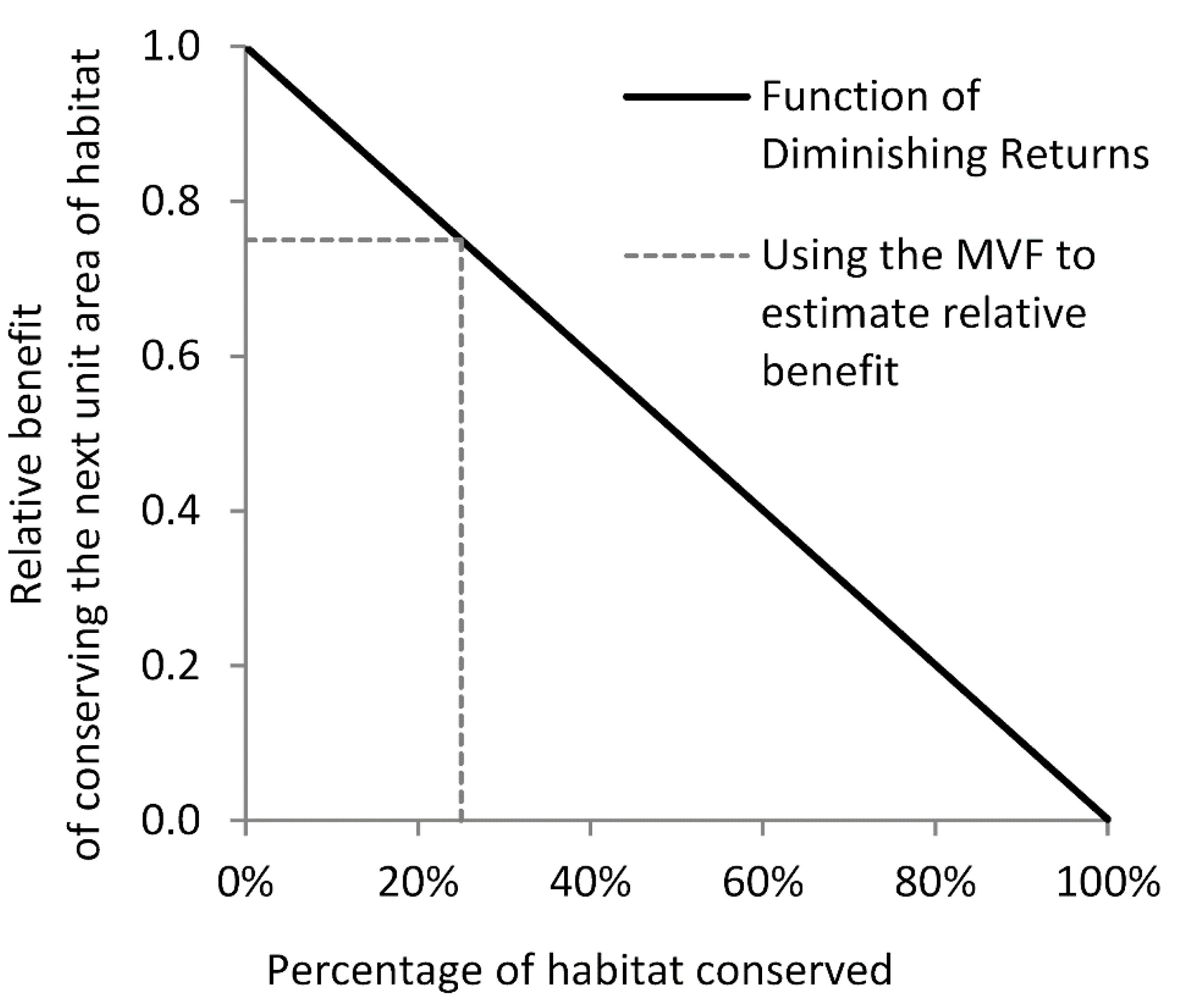
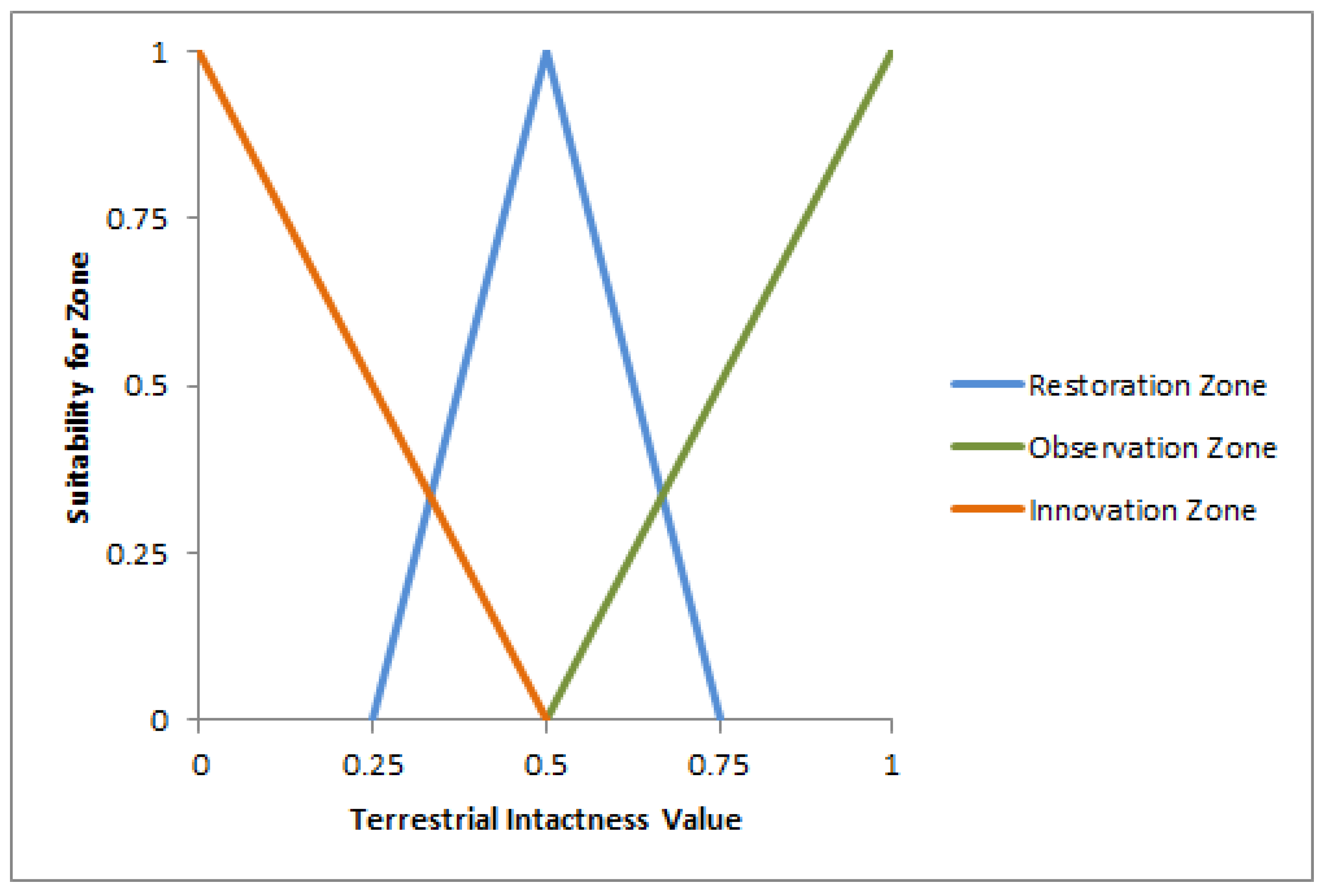
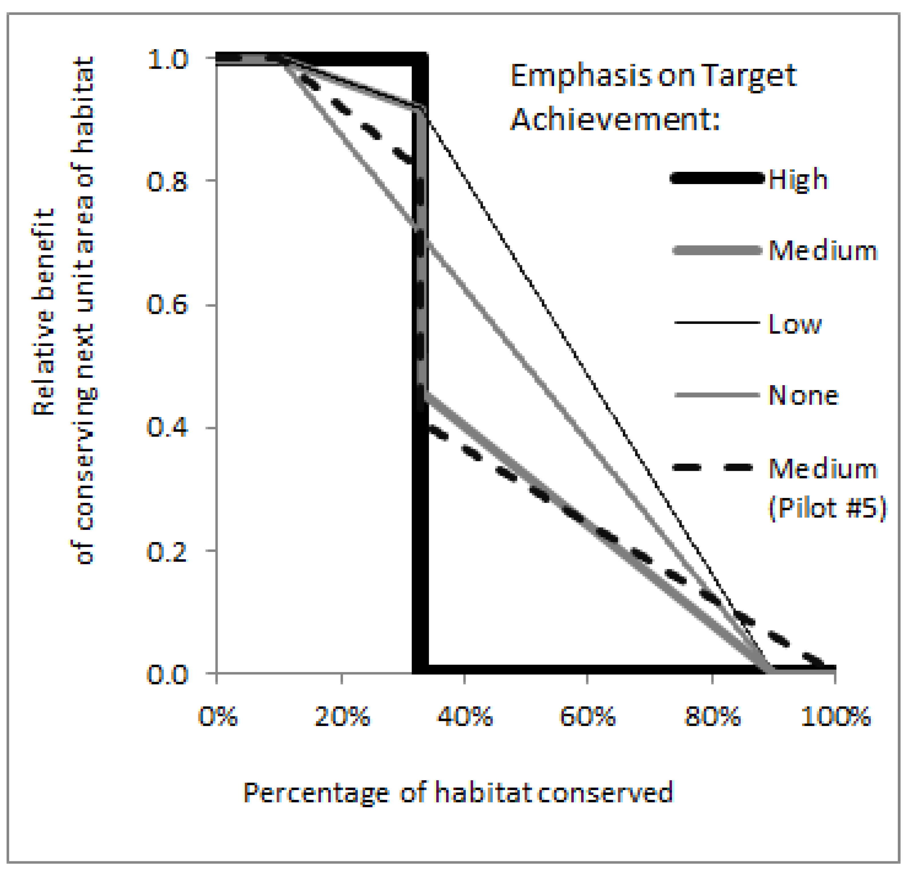
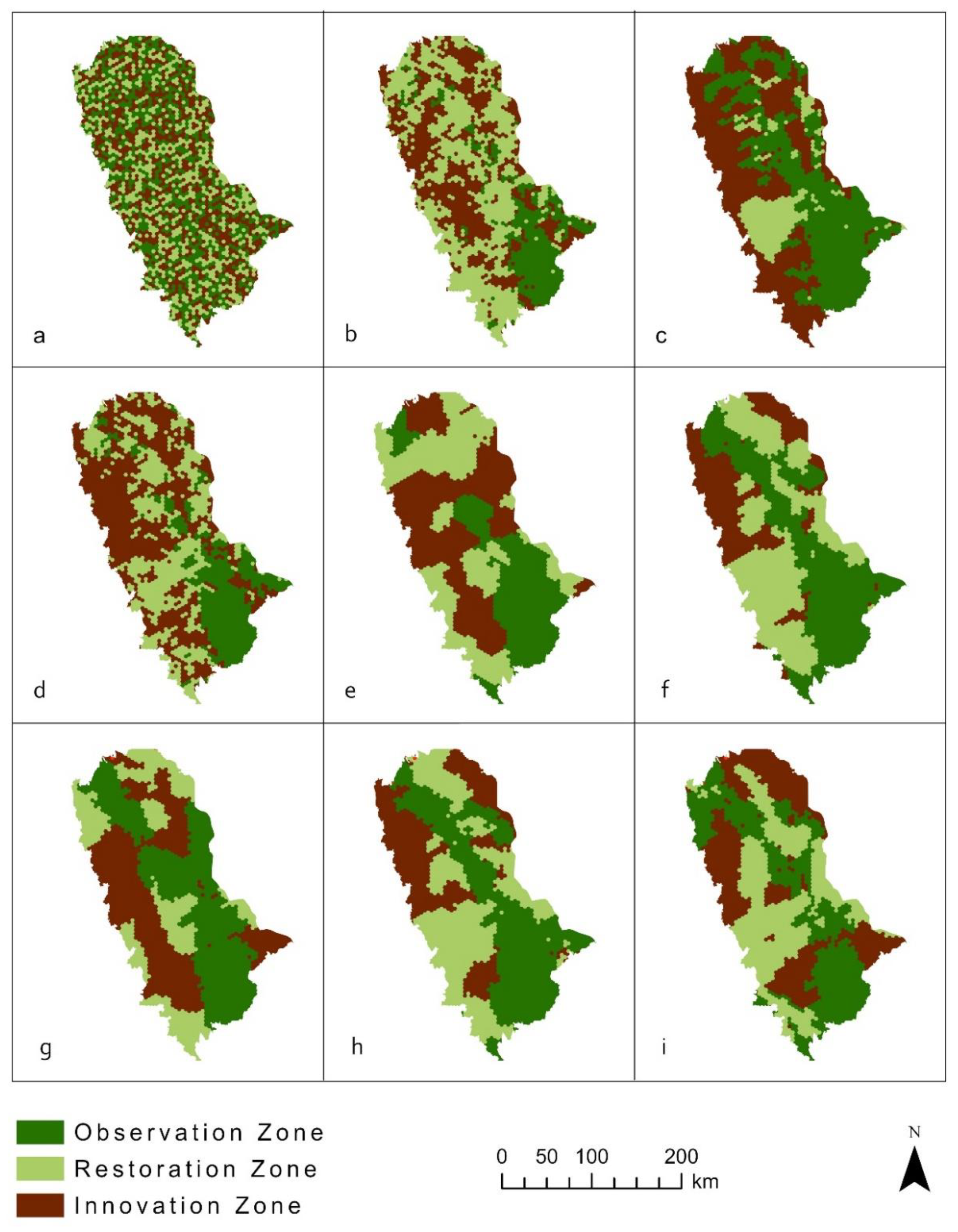
Table 1.
The suitability and socio-political influence values for each designation.
| Designation or Area | Suitability for | Socio-Political Influence | ||
|---|---|---|---|---|
| Observation Zone | Restoration Zone | Innovation Zone | ||
| Wilderness Areas (USFS and NPS) | 0.9 | 0.05 | 0.05 | 0.96 |
| CalFIRE WUI Fire Zone | 0 | 0.34 | 0.66 | 0.95 |
| Wild River Corridor | 0.75 | 0.19 | 0.07 | 0.78 |
| Recommended Wilderness Areas (USFS) | 0.8 | 0.13 | 0.07 | 0.78 |
| Research Natural Area | 0.88 | 0.07 | 0.05 | 0.72 |
| USFS Experimental Forest and Range | 0.11 | 0.21 | 0.69 | 0.66 |
| Inventoried Roadless Area (USFS) | 0.62 | 0.24 | 0.15 | 0.62 |
| Scenic River Corridor | 0.43 | 0.37 | 0.19 | 0.5 |
| Primitive Non-Motorized Area | 0.69 | 0.23 | 0.09 | 0.37 |
| Semi-primitive Motorized Area | 0.34 | 0.39 | 0.26 | 0.31 |
| Recreational River Corridor | 0.32 | 0.47 | 0.2 | 0.31 |
| Citizen Inventoried Roadless Area | 0.6 | 0.28 | 0.13 | 0.3 |
| Semi-primitive Non-Motorized Area | 0.56 | 0.27 | 0.2 | 0.27 |
Table 2.
The weights and parameter that varied for the five non-basic allocation scenarios.
| Criterion | Even Weighted | Designations Skew | Pre-Assign Wilderness, Even Weighted | Pre-Assign Wilderness, Designations Skew | Pre-Assign Wilderness, Connectivity Skew | |
|---|---|---|---|---|---|---|
| Should Wilderness be pre-assigned to Objective 1? | No | No | Yes | Yes | Yes | |
| Weights: | ||||||
| Old Growth Suitability | 0.33 | 0.25 | 0.33 | 0.25 | 0.25 | |
| Naturalness | 0.33 | 0.5 | 0.33 | 0.5 | 0.5 | |
| Fire Return Interval Departure | 0.34 | 0.25 | 0.34 | 0.25 | 0.25 | |
| Ecological Condition | 0.33 | 0.3 | 0.33 | 0.3 | 0.4 | |
| Designations | 0.33 | 0.6 | 0.33 | 0.6 | 0.4 | |
| Fire - Wildland Urban Interface | 0.34 | 0.1 | 0.34 | 0.1 | 0.2 | |
| Elevation Representation | 0.33 | 0.5 | 0.33 | 0.5 | 0.5 | |
| Subregion Representation | 0.33 | 0.2 | 0.33 | 0.2 | 0.2 | |
| Vegetation Representation | 0.34 | 0.3 | 0.34 | 0.3 | 0.3 | |
| Composition Value | 0.5 | 0.8 | 0.5 | 0.8 | 0.5 | |
| Representation Value | 0.5 | 0.2 | 0.5 | 0.2 | 0.5 | |
| Connectivity | 0.5 | 0.8 | 0.5 | 0.8 | 0.8 | |
| Adjacency | 0.5 | 0.2 | 0.5 | 0.2 | 0.2 | |
| Representative Composition | 0.5 | 0.5 | 0.5 | 0.5 | 0.5 | |
| Spatial Context | 0.5 | 0.5 | 0.5 | 0.5 | 0.5 | |
| Linkage Length | 0.25 | 0.0 | 0.25 | 0.0 | 0.2 | |
| Linkage Permeability | 0.25 | 0.5 | 0.25 | 0.5 | 0.4 | |
| Values of Core Areas Linked | 0.25 | 0.0 | 0.25 | 0.0 | 0.0 | |
| Climate Signature Difference of Cores | 0.25 | 0.5 | 0.25 | 0.5 | 0.4 | |
| Core Area Habitat Quality | 0.33 | 0.5 | 0.33 | 0.5 | 0.5 | |
| Core Area Size | 0.33 | 0.25 | 0.33 | 0.25 | 0.25 | |
| Core Area Shape | 0.34 | 0.25 | 0.34 | 0.25 | 0.25 | |
Table 3.
The Evaluation Scores, and associated Performance Metric Scores, for the nine scenarios.
| Version Name | Evaluation Score | Composition Suitability Score | Representation Score | Connectivity Score | Adjacency Score | Wilderness in Observation Zone |
|---|---|---|---|---|---|---|
| Random Scenario | 0.000 | 0.000 | 0.492 | 0.000 | 0.000 | 0.000 |
| Ecological Scenario | 0.443 | 0.921 | 0.565 | 0.352 | 0.146 | 0.000 |
| Designations Scenario | 0.667 | 0.752 | 0.000 | 0.558 | 0.428 | 1.000 |
| Suitability Scenario | 0.640 | 1.000 | 1.000 | 0.419 | 0.231 | 0.000 |
| Even Weighted Run | 0.803 | 0.649 | 0.550 | 1.000 | 1.000 | 0.000 |
| Designations Skew | 1.000 | 0.623 | 0.683 | 0.772 | 0.784 | 1.000 |
| Pre-Assign Wilderness v1, (Even Weights) | 0.891 | 0.536 | 0.182 | 0.893 | 0.883 | 1.000 |
| Pre-Assign Wilderness v2, (Designations Skew) | 0.960 | 0.655 | 0.689 | 0.673 | 0.709 | 1.000 |
| Pre-Assign Wilderness v3, (Connectivity Skew) | 0.909 | 0.572 | 0.597 | 0.781 | 0.604 | 1.000 |
Publisher’s Note: MDPI stays neutral with regard to jurisdictional claims in published maps and institutional affiliations. |
© 2020 by the authors. Licensee MDPI, Basel, Switzerland. This article is an open access article distributed under the terms and conditions of the Creative Commons Attribution (CC BY) license (http://creativecommons.org/licenses/by/4.0/).
Share and Cite
MDPI and ACS Style
Gallo, J.A.; Aplet, G.H.; Greene, R.; Thomson, J.L.; Lombard, A.T. A Transparent and Intuitive Modeling Framework and Software for Efficient Land Allocation. Land 2020, 9, 444. https://doi.org/10.3390/land9110444
AMA Style
Gallo JA, Aplet GH, Greene R, Thomson JL, Lombard AT. A Transparent and Intuitive Modeling Framework and Software for Efficient Land Allocation. Land. 2020; 9(11):444. https://doi.org/10.3390/land9110444
Chicago/Turabian StyleGallo, John A., Gregory H. Aplet, Randal Greene, Janice L. Thomson, and Amanda T. Lombard. 2020. "A Transparent and Intuitive Modeling Framework and Software for Efficient Land Allocation" Land 9, no. 11: 444. https://doi.org/10.3390/land9110444
Note that from the first issue of 2016, this journal uses article numbers instead of page numbers. See further details here.