Refining the Tiered Approach for Mapping and Assessing Ecosystem Services at the Local Scale: A Case Study in a Rural Landscape in Northern Germany

Abstract

Spatially explicit assessments of ecosystem services (ES) potentials are a key component in supporting a sustainable land use management. The ES matrix method is a commonly used approach as it allows for a comparably fast, comprehensible and accessible ES assessment. As it is often based on land use/land cover data (LULC) with no spatial variability, a main critique is that the results fail to assess spatial variability at landscape levels, which limits the reliability of the outputs for spatial planning applications. By using the case study area of Bornhöved in northern Germany, we analyzed three assessment methods that combine expert judgments, LULC data with different resolutions and ecosystem condition indicators, in order to find the required resolution and data for ES assessment and mapping at a local scale. To quantify map discrepancies, we used the structural similarity index (SSIM) and analyzed the differences in local mean, variance and covariance between the maps. We found that using different spatial resolutions led to a relatively small difference in the outcomes, in which regulation and maintenance services are more affected than the other services categories. For most regulation, maintenance and cultural ES, our results indicate that assessments based only on LULC proxies are not suitable for a local quantitative assessment of ES, as they cannot sufficiently cover the spatial heterogeneity of ES capacities that arise from different ecosystem conditions.

1. Introduction

Ecosystem services (ES) are defined as the benefits that ecosystems provide in support of human well-being [1]. ES assessment and mapping have become popular approaches for sustainable planning and management of natural resources, for instance in EU policies [2,3]. ES approaches can also help to preserve and enhance landscape multifunctionality [4,5]. Different methodologies have been developed for assessing and mapping ES (for a review see [5]), that can be classified in three mdifferent tiers [6]. The appropriate ES assessment methods or tier depend on the purpose of the assessment (e.g., research or policy questions). The first tier includes simple methods that establishes binary links between LULC, and ES scores obtained from previous studies or based expert knowledge approaches: experts are asked to rank LULC classes according to the potential of these classes to supply an ES. The second tier includes the methodologies that rely on information about relationships between indicators and ES, mainly obtained from literature. Methodologies of the third tier extrapolate ES estimates of primary data and quantitative regression model approaches. Depending on the research question, a Tier 1 approach can be used to provide a rough overview of a phenomenon or for awareness raising. However, a Tier 3 is needed to support local planning decisions. For an assessment of multiple ES, the Tiers 2 and 3 are hardly applicable, as higher Tier approaches are usually more data-intensive. This is particularly the case for an ES assessment adapted to local characteristics, for which regressions and socio-ecological system models set in another region of the world cannot be applied without adjustments.

One commonly used method for ES potential assessment is the ES matrix approach by Burkhard et al. [7,8,9] (Tier 1 to 2), in which ES “potential” was defined as the capacity of an ecosystem to deliver ES based on ecological properties and functions, independent of an actual demand for these services [10]. With the ES matrix approach, the ES potential of a landscape can be estimated based on various ES quantification approaches [11]. Expert scorings of ES potentials—in combination with geospatial units such as LULC types—are one of the most commonly used approaches in ES matrix applications [12,13]. Thus, LULC types are used as basic units for the capacity of a given area to supply ES, under the assumption that there are explicit causal relationships between LULC types and the delivery of ES. The ES matrix approach is a tool for decision support in sustainable resource management as it is highly adaptable to various socio-ecological system settings, easily accessible and enables an efficient and relatively fast comprehensible assessment [14]. This method allows the spatial modelling and mapping of multiple ES at different scales and reflects the multifunctionality of landscapes, i.e., the capacity of different ecosystem types within a landscape to provide a broad range of ES.

ES matrix models are often used along with CORINE land cover data (CLC) [12,15], as this dataset is freely accessible, is regularly updated by the European Environmental Agency and covers all EU member states. A landscape analysis based on LULC may be adequate for some ES and ecosystems, e.g., heavily human-managed ecosystems dedicated to the production of one or a few services [16]. This is particularly the case for biomass production in forests or food production in croplands, as these ecosystems mainly rely on human inputs and less on natural processes (via e.g., the selection of plant and animal species, the use of fertilizers and pesticides, irrigation water input, energy and labor use). However, the CORINE dataset is quite coarse (usually 25 ha minimum mapping unit (MMU)) and may not be suitable for local-scale assessments, as semi-natural elements, small habitats but also transport networks are not well identified in this dataset. Moreover, the assessment of non-target ES or non-marketed ES such as many regulation services is generally more challenging than the valuation of provisioning ES [10]: the supply of most of the regulation ES depends on several ecosystem structures and processes, which often occur over larger spatial and temporal scales. There is also a considerable lack of knowledge on the mechanisms of the processes underlying the supply of these services [17,18,19]. Moreover, regulation and maintenance ES supply usually varies considerably within one land cover type [14,20,21,22] and depends on additional ecosystem conditions such as vegetation cover and biodiversity, soil types and texture or water availability [23,24]. Cultural ES potentials usually also depend on a complex mix of biophysical and anthropogenic landscape characteristics such as topography, presence of species and accessibility. Thus, regulation and maintenance and cultural ES tend to rely on additional ecological and management features and may not be appropriately assessed solely based on LULC proxies.

This summarizes two of the main critiques in regard to LULC-based approaches. First, CLC data are too coarse for an accurate ES assessment supporting local decision-making processes [22,25,26]. Second, ES assessments cannot be done simply based on LULC data as the assessment tends to be not accurate enough to catch spatial variability within individual land cover classes and between landscapes [13,14,22]. Accuracy is defined as how well a model estimates the true distribution of a phenomenon [16]. The accuracy of a model partly depends on its capacity to capture ES heterogeneity, i.e., the “degree of spatial variation within the spatial distribution of an ES”, so on how ES potential relies on ecosystem conditions [16]. The application of a suitable method for modelling heterogeneous ES potentially increases the accuracy of the outputs, but it usually requires more effort and increases information costs. Furthermore, different research questions or mapping issues require different resolutions.

This paper explores how different levels of spatial resolution and ES matrix assessment complexity impact the outcomes of a local-scale analysis by applying three different levels of assessment. Using the ES matrix approach, we first examine how spatial resolution influences the assessment by comparing predicted ES potentials based on the open-access CLC dataset with the ATKIS (authoritative topographic and cartographic information system)/InVeKoS (Integrated Administration and Control System) datasets, which have a finer spatial resolution and include small habitats and landscape elements. We then select and calculate ecosystem condition indicators based on the fifth mapping and assessment of ecosystems and their services (MES) report (http://biodiversity.europa.eu/mes) to develop an ecosystem condition index. This assessment level combines the resulting index with the ES potential matrix to analyze how data on ecosystem condition influence the outputs of ES assessments. We applied these three assessment methods in a case study area in northern Germany.

The following three research questions are addressed in this study:

• How does a higher spatial resolution with more information on small landscape elements affect the results of an ES-matrix assessment on a local scale?
• Does the integration of ecosystem condition information add value to the ES assessment and can patterns between different ES and ES categories be detected?
• What conclusions can be drawn for practical applications in landscape management?

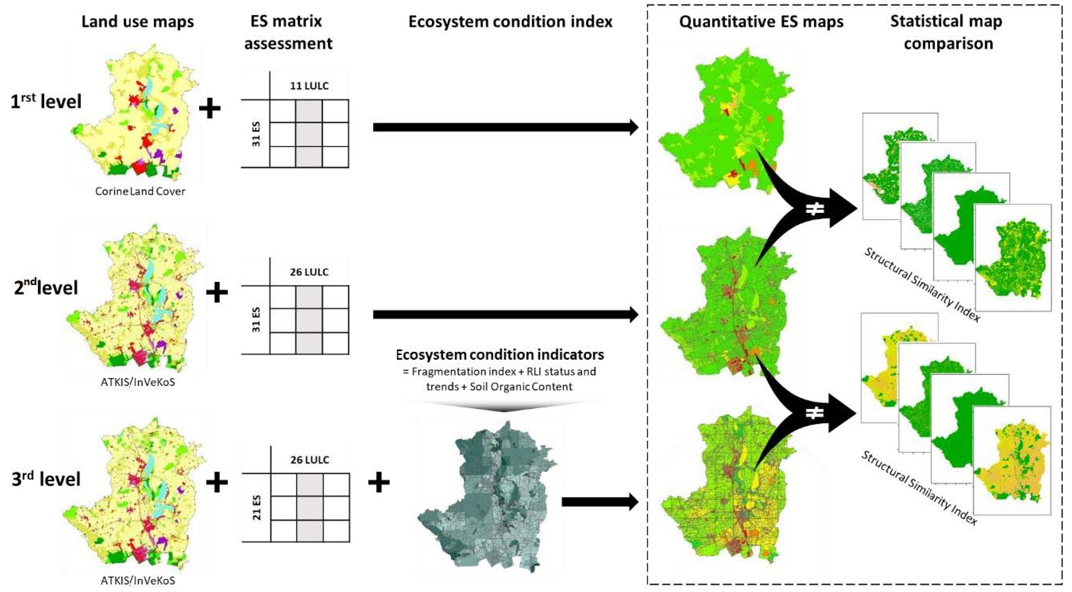
2. Material and Methods

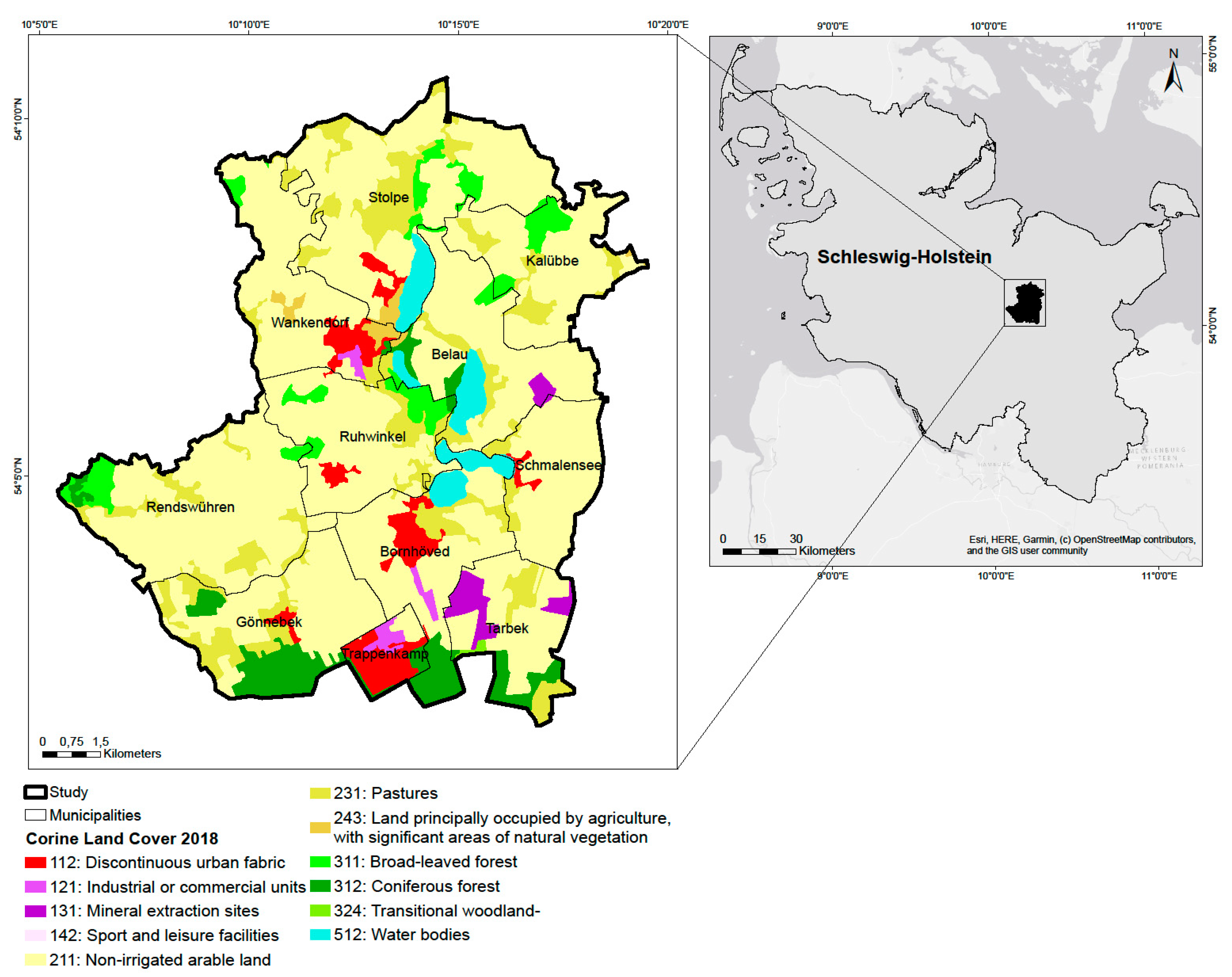
2.1. Case Study Area (CSA)

The CSA is located in the region of the Bornhöved Lake District in the province of Schleswig–Holstein in northern Germany (Figure 1). It was the focus of a former integrative ecological study project and is a long-term ecological research (LTER) site. The present study area is bigger than the former LTER site and includes the administrative borders of the constitutive municipalities, resulting in a CSA of 147 km². Agroecosystems dominate the landscape in a catchment area of five glacially formed and consecutively connected lakes. The CSA is composed of relatively small and diverse ecosystems, as well as a high proportion of hedgerows, shaping a highly diverse and fragmented landscape (see Figure 1 and [27]). The former LTER site was used in several ES assessments focusing on one single ES [28] or a group of ES [7,8,9,26].

2.2. Ecosystem Services Assessments

To guide through the following section, we introduce the workflow of the different levels of assessment developed in this study. Figure 2 illustrates this workflow and how the different datasets are integrated in the different levels of assessment. We prepared two geospatial maps using three different datasets: the CLC datasets for the first assessment level, the ATKIS and InVeKoS datasets were combined for the second and third assessments. We used the LULC classes from the three datasets to build a unique ES matrix based on a common typology and solicited local experts. For the first and second level assessment, we applied the resulting matrix to the different geospatial datasets to map ES potential in the CSA. For the third level assessment, we added ecosystem condition indicators to the analysis: ES potentials were calculated based on the environmental condition scores of each ecosystem and the ES scores from the matrix. Finally, we statistically compared the different levels of assessment and the differences in the resulting ES potential maps.

2.2.1. Geospatial Datasets

The LULC typology used for the first level assessment is derived from the CLC 2018 dataset (https://land.copernicus.eu/pan-european/corine-land-cover/clc2018).

The geospatial dataset used in the second level assessment is composed of ATKIS (version 2012) and improved by using InVeKoS data (version 2010). ATKIS is a national standardized topographic information system provided by the German Federal Surveying Authorities. InVeKoS is a control system established by the European Commission to control payments of income support from the European Common Agricultural Policy to farmers. Both datasets feature an object-based comprehensive description of the Earth’s surface. Topographical and LULC features are modeled as points, polylines or polygons. The spatial resolution of these two datasets depends on the feature classes and has a MMU between 0.1 and 1 hectare [29] compared to the 25 hectares of CLC.

The two datasets differ in represented LULC classes: “transitional woodland-shrub” and “land principally occupied by agriculture, with significant areas of natural vegetation” from the CLC dataset are not part of the ATKIS/InVeKoS classification systems. The CLC class “transitional woodland/shrub” corresponds to “areas representing natural development of forest formations, consisting of young plants of broad–leaved and coniferous species, with herbaceous vegetation and dispersed solitary adult trees. Transitional process can be for instance natural succession on abandoned agricultural land, regeneration of forest after damages of various origin (e.g., storm, avalanche), stages of forest degeneration caused by natural or anthropogenic stress factors (e.g., drought, pollution), reforestation after clearcutting, afforestation on formerly non-forested natural or semi-natural areas, etc.” (https://land.copernicus.eu/user-corner/technical-library/corine-land-cov er-nomenclature-guidelines/html/index-clc-324.html). The CLC class “land principally occupied by agriculture, with significant areas of natural vegetation” is defined as “areas principally occupied by agriculture, interspersed with significant natural or semi-natural areas (including forests, shrubs, wetlands, water bodies, mineral outcrops) in a mosaic pattern.” (https://land.copernicus.eu/user-cor ner/technical-library/corine-land-cover-nomenclature-guidelines/html/index-clc-243.html).

Table 1. Differences in land use/land cover data (LULC) classes shares in the study area in 2018 (CLC) and 2010 (ATKIS/InVeKos) for the two LULC datasets.

CLC Level 2	CLC Level 3 Classes	Corresponding ATKIS/InVeKoS Classes	% Total ATKIS/InVeKoS	% Total CLC Level 3
Arable land	Non–irrigated arable land	Arable land	59.81%	67.25%
		Fallow land	0.36%
		Truck farm	0.48%
Permanent crops	Fruit trees and berry plantations	Fruit trees and berry plantations	0.02%
Pastures	Pastures	Pastures	11.76%	13.12%
Heterogeneous agricultural areas	Land principally occupied by agriculture, with significant areas of natural vegetation	–		0.84%
	–	Hedgerows	2.36%
	–	Tree rows	0.21%
	–	Copse, thickets	0.15%
	–	Single trees	0.08%
	–	Field borders	0.11%
Forests	Broad–leaved forest	Broad–leaved forest	3.34%	4.22%
	Coniferous forest	Coniferous forest	3.85%	4.95%
	Mixed forest	Mixed forest	3.48%
Scrub and/or herbaceous vegetation associations	Transitional woodland–shrub	–		0.10%
	Sclerophyllous vegetation	Sclerophyllous vegetation	0.33%
Open spaces with little or no vegetation	Sparsely vegetated areas	Sparsely vegetated areas	0.17%
Urban fabric	Continuous housing area	Continuous housing area	3.15%
	Discontinuous urban fabric	Discontinuous housing area	1.65%	4.32%
Industrial, commercial and transport units	Industrial or commercial units	Industrial and commercial units	0.99%	0.72%
	Airports	Airports	< 0.01%
	Road and rail network	Rail network	0.09%
		Road network	2.32%
Mine, dump and construction sites	Mineral extraction sites	Mineral extraction sites	0.89%	1.41%
	–	Paths	0.52%
Artificial, non-agricultural vegetated areas	Sport and leisure facilities	Sport and leisure facilities	0.61%	< 0.01%
Inland waters	Water courses	Water courses	0.08%
	Water bodies	Water bodies	3.70%	3.07%
	–	Ditch	0.35%
Inland wetlands	Inland marshes	Wetlands	0.08%

and Figure 3 show all LULC classes and their respective proportions for each LULC dataset are shown in Table 1. The main differences between CLC and ATKIS/InVeKoS are found in the higher number of LULC classes and also in total surface covered by “arable land”, by landscape elements (LULC subclass which regroups the classes “hedgerows”, “tree rows”, “copse, thickets”, “single trees”, “field borders”) as well as by artificial surfaces.

2.2.2. ES Matrix Approach

The ES matrix approach by Burkhard et al. [7,8,9] is based on a look-up table where the capacity of each geospatial unit (e.g., LULC types) to supply ES is quantified. In this study, we assessed the ES potential of the different LULC classes. We did not consider the actual use or flow of ES, nor the demand for ES (see Syrbe et al. [30] for definitions of ES potential, stock, use and demand). ES potentials are scored on a scale from zero (no relevant potential) to five (very high relevant potential). The methodology is also described in Burkhard and Maes [31] and in Campagne and Roche [13]. We adhered to the following steps: (1) identification of the relevant ES and ecosystems to be assessed, (2) selection of an expert panel, (3) collection of expert scorings and (4) compilation of the final matrix values.

The list of ES in the matrix is based on the common international classification of ecosystem services (CICES V5.1) [32] and covers all three main CICES sections, i.e., regulation and maintenance ES, provisioning ES and cultural ES. Each ES is briefly explained in the matrix in the supplement materials (Table 1). The list of ecosystems corresponds to the CLC, ATKIS and InVeKoS LULC classes in the CSA (see Table 1 “Corresponding ATKIS/InVeKoS classes”). The experts had a wide range of ES and ecosystems expertise, had researched the study area and were familiar with ES concepts.

Müller et al. [33] developed an ES assessment matrix for CLC land cover classes within the German Federal State of Schleswig–Holstein, to which more than 55 experts contributed. We used this matrix for the first ES assessment, as all the selected ES and LULC were scored in this matrix. For the second assessment, we completed the matrix with all the missing LULC, i.e., the LULC classes within the ATKIS/InVeKoS datasets that were not represented in CLC classes. These classes were assessed through a new evaluation process, in which several preliminary discussion rounds were organized with four experts in order to identify in the missing values of the matrix. Other experts were then contacted by email and asked to modify the potential scores in the preliminary matrix in case of differing opinions (only for the LULC classes missing in the matrix from Müller et al. [33]). Materials that were provided to experts included a map of the CSA as well as a matrix. In total, 10 local experts in environmental management, soil, ecology, agriculture and climate sciences contributed to the new assessment. The final matrix included 31 LULC classes and 34 ES and can be found in the supplement materials (Table 1).

2.2.3. Ecosystem Condition Indicators

Selecting Suitable Indicators

The MAES working group of the European Commission (http://biodiversity.europa.eu/maes) aims at providing support to the EU member states in regard to ES mapping and assessment [34]. The fifth MAES report presents a list of key indicators for mapping and assessing ecosystem condition of the main ecosystem types at the European level [35]. From this report, we selected ecosystem condition key indicators for which we could find local data or easily develop an equivalent that was spatially explicit and sensitive to local land use change. Whereas MAES provides one list of indicators per ecosystem type, the indicators selected for this study are not ecosystem type-dependent and are relevant for artificial areas, agroecosystems, forests as well as other natural and semi-natural ecosystems. Three indicators were selected: the landscape fragmentation index, a Red List Index for ecosystems and the soil and organic carbon (SOC) (

Table 2. Overview of the data used as ecosystem condition indicators.

	Indicators	References	Spatial Resolution
Ecosystem attributes	Landscape fragmentation index	EEA landscape fragmentation per km (mesh)	1 km2
	Red List Index for ecosystems	Schleswig–Holstein Red Lists and ATKIS/InVeKoS LULC classes	Variable (from +/- 3 m to less than 1 ha as ATKIS and InVeKoS resolution)
Structural soil attributes	Soil organic carbon (SOC)	Federal Institute for Geosciences and Natural Resources (BGR)	0.25 km2

).

Landscape Fragmentation Index

Landscape fragmentation results from the transformation of large natural and semi-natural ecosystems into smaller and isolated, fragmented ecosystems [36]. This process can for instance be caused by the construction of transport networks and built-up areas, which have greatly expanded over the last 50 years. Accessibility is a prerequisite for the exploitation and supply of a wide range of ES. Up to a given density, there is a positive relationship between road density and the potential use of provisional and cultural services, as it generally depends on access to the ES supply areas. However a high fragmentation has a negative impact on agricultural and timber production, as small land parcels tend to have lower yields [36]. Transportation networks also have negative impacts on cultural ES, above all for recreational use and landscape aesthetics. Fragmentation seriously affects regulation ES by, among other, species movement impediment and habitat reduction [37], water cycle disruption [38] and erosion phenomenon exacerbation [38]. A detailed list of the effects of fragmentation on ecosystem conditions and services can be found in the report of the European Environment Agency (EEA) [36].

The EEA applied the method of effective mesh density to measure the degree of landscape fragmentation in the EU member states [36]. This landscape metric unit is based on the probability that two points chosen randomly in an area are connected and not separated by any natural or man-made barriers. The effective mesh size represents the degree of fragmentation of a landscape: the smaller the value, the more fragmented the landscape. The datasets used to calculate the mesh are CLC (2006) for artificial areas such as urban and industrial units but also waterbodies, TeleAtlas Multinet for the roads and railroads, WorldClim and Nordregio for topographic and climatic barriers [36]. The resulting map presents landscape fragmentation at 1 km² resolution.

Local Red List Index

The Red List Index (RLI) is one prominent indicator in the Convention for Biological Diversity (CBD) indicator sets for biodiversity conservation [39], but has until now not been used for ES assessments. RLI is a key condition indicator in the fifth MAES report that indicates “conservation status and trends of species of community interest” and “conservation status and trends of habitats of community interest” [35] and that aims at supporting the evaluation of the efficiency of conservation policies. The RLI measures status and trends in the overall extinction risk of species by using weight scores based on the Red List status of each assessed species, which range from 0 (least concern) to 5 (extinct/extinct in the wild). To date, global RLIs have been calculated for birds, mammals, amphibians, corals and cycads [40]. They serve as indicators to evaluate progress towards meeting the CBD “2010 biodiversity target” and help to develop a better understanding of which taxa, regions or ecosystems are declining or improving globally. Global RLIs and Red List assessments are hardly sensitive to local land-use management and decisions, so we instead used local extinction risk assessments lists provided by the State Agency for Nature and Environment of Schleswig–Holstein [41,42,43]). Moreover, as we needed a spatially explicit indicator, we calculated local RLIs for each ecosystem and not for each species group, following the method by Juslén et al. [44]. Each species was associated to one or more ecosystems based on their habitats described in national or Schleswig–Holstein Red List assessments. A total of 214 species of birds, 44 mammals and 18 amphibians and reptiles were included in the assessment.

The RLI values were calculated following the method developed by Butchart et al. [40]. We multiplied the number of taxa in each ecosystem by the category weight (0 for least concern, 1 for near threatened, 2 for vulnerable, 3 for endangered, 4 for critically endangered and 5 for extinct/extinct in the wild). These products are summed up and then divided by the number of taxa multiplied by the maximum weight 5, the “maximum possible denominator”, which corresponds to the “worst case scenario”. To obtain the RLI value, this sum is subtracted from 1. The resulting index varies between zero and one: the lower the value, the closer the set of taxa living in the ecosystem is heading towards extinction. The Red List status of the pool of species living in an ecosystem is used as a proxy for this ecosystem condition. To make this indicator sensitive to land management change, we included the RLI value trends as well as the values from the last Red List assessment. The “RLI status” corresponds to the values from the last Red List assessment. The “RLI trend” corresponds to the difference between the last and the first Red List assessment values (i.e., RLI status—RLI 1990 (or 1995)) for each ecosystem.

Soil Organic Carbon (SOC)

Soil is a key component of terrestrial ecosystems and plays an essential role in ecosystem functioning [45]. Despite its importance, relatively little emphasis has been placed on soil in studies that map ES, mainly because our understanding on how soils support ES delivery is incomplete [46,47]. Soil quality and its capacity to provide a wide range of ES depend on key properties such as soil type and texture, soil organic carbon content, pH, soil porosity and structure [48,49,50]. Soil organic carbon (SOC) is mainly determined by the balance between net primary production and the rate of decomposition of organic material, which both depend on land use, climate and microorganism action. A literature review showed that SOC can be (directly or indirectly) linked to a broad range of ES, in all three ES CICES categories [48]. As no map was readily available at the desired local scale, we developed a SOC map based on the data and method from the Federal Institute for Geosciences and Natural Resources’ (BGR) soil information system (FISBo), which provides soil information at land and national scale [51,52]. The method from the BGR allows to determine the SOC from soil characteristics, climatic data and land cover types.

2.3. ES Potential Maps

2.3.1. First and Second Level

Ecosystem mapping was carried out for the CSA using CLC (first assessment level) and ATKIS/InVeKoS (second assessment level) datasets. All spatial analyses were executed using ArcGis 10.6.1. ES potential maps were obtained by joining each LULC map with the ES potential matrix. Exemplary ES potential maps (crop production, pollination and recreation and tourism) are presented in the results, the other maps can be found in the Supplementary Materials.

2.3.2. Third Level

For the third level assessment, we assume that good ecosystem condition is prerequisite for a high supply of ES [35] and therefore first combined the three selected indicators into one ecosystem condition map (Figure S1). However, most provisioning ES, such as agricultural production (crop, livestock, biomass for energy, fodder and fiber production) but also timber production, often arise much more from human interventions than from ecological properties and functions of the ecological system [53] (but see Balvanera et al. [54] and Harrison et al. [55]). Some ecosystem properties have a direct positive impact on agricultural production, but it can be generally substituted by human actions. For example, a high SOC maximizes crop and pasture biomass. A low SOC can be however compensated by adding off-farm organic residues. As we cannot assume that the potential of agricultural and timber production services increases with ecosystem conditions, we did not include them into the third assessment level.

A second assumption, in the absence of further evidence [19], was that each indicator equally contributes to the ecosystem condition of each ecosystem type except aquatic ecosystems for which the SOC is not relevant, following the Equation (1):

$$\mathrm{EC} =\frac{1}{4}\left(\mathrm{FI} +{ \mathrm{RLI}}_{\mathrm{trend}} +{ \mathrm{RLI}}_{\mathrm{status}} + \mathrm{SOC}\right)$$

(1)

where EC is the aggregated indicator value for the ecosystem condition, FI the fragmentation index, RLI_status the RLI for Schleswig–Holstein for 2014 and RLI_trend the improvement or degradation of the RLI over the years, SOC the soil organic content. All indicators are scaled down to the interval [0,1], to give all the indicators an equivalent weight. The EC values are also scaled into the range [0,1]. EC values from zero (the ecosystem is in a very bad condition) and one (the ecosystem is in a very good condition).

As the SOC is not relevant for aquatic ecosystems, we did not include this indicator in the EC of water bodies nor water courses. For these ecosystems, Equation (2) is defined as follows:

$$\mathrm{EC} =\frac{1}{3}\left(\mathrm{FI} +{ \mathrm{RLI}}_{\mathrm{trend}} +{ \mathrm{RLI}}_{\mathrm{status}}\right)$$

(2)

The ecosystem capacity to deliver ecosystem services is determined by the ecosystem condition, following Equation (3):

$${\mathrm{ES}}_{\mathrm{potential}} = \mathrm{EC}\times \mathrm{ES}$$

(3)

where ES_potential is the calculated ecosystem services potential resulting from the ecosystem condition (EC) and the ES potential scores (ES) from the matrix.

2.4. Influence of Typology and Resolution

The CLC and ATKIS/InVeKoS datasets use different typologies to describe some of the LULC classes. The differences in the ES maps resulting from the different LULC datasets are therefore not only due to different resolutions, but also to a difference in typologies. To differentiate these two effects, we compared the two maps using the Union tool from ArcGIS. The resulting map is a map containing each input feature from the two LULC datasets, associated with its attributes. The resulting attribute table shows how the two datasets overlap and this allowed to determine which CLC LULC classes corresponds to each ATKIS/InVeKoS class. Using this attribute table, we then calculated the percentage of each CLC class, which was classified (or not) to the corresponding ATKIS/InVeKoS class (see Table 1). To assess the effect of spatial resolution, we assessed the percentage of LULC classes that were misclassified according to the size of each feature.

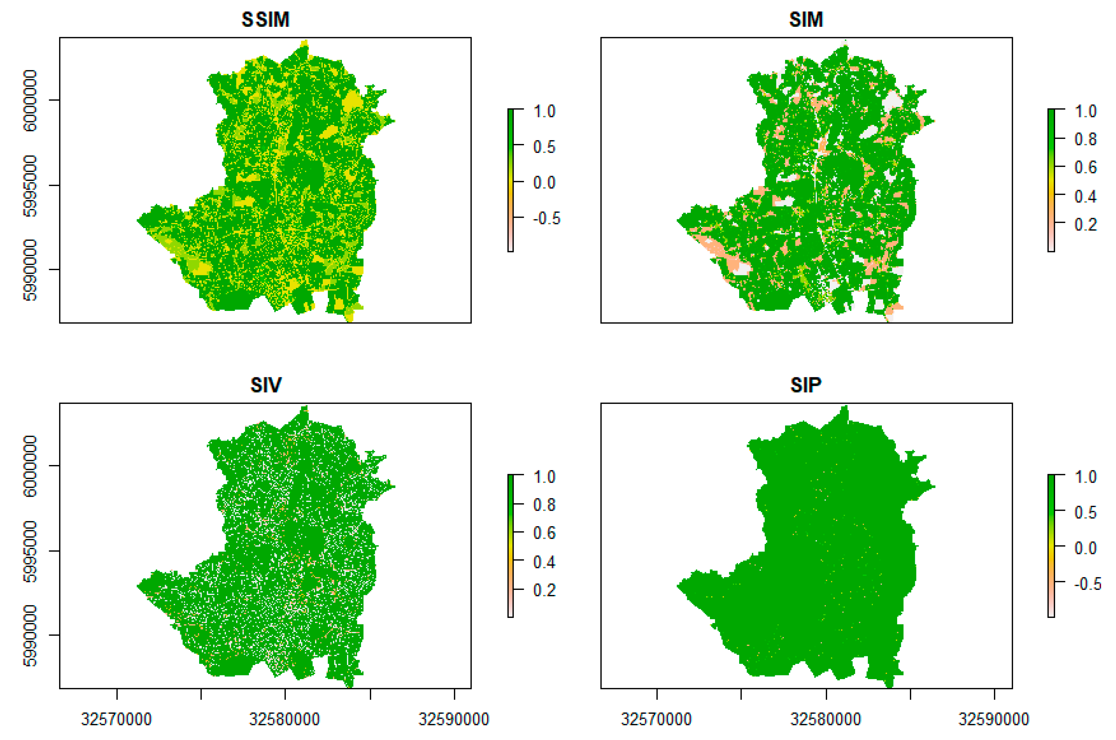
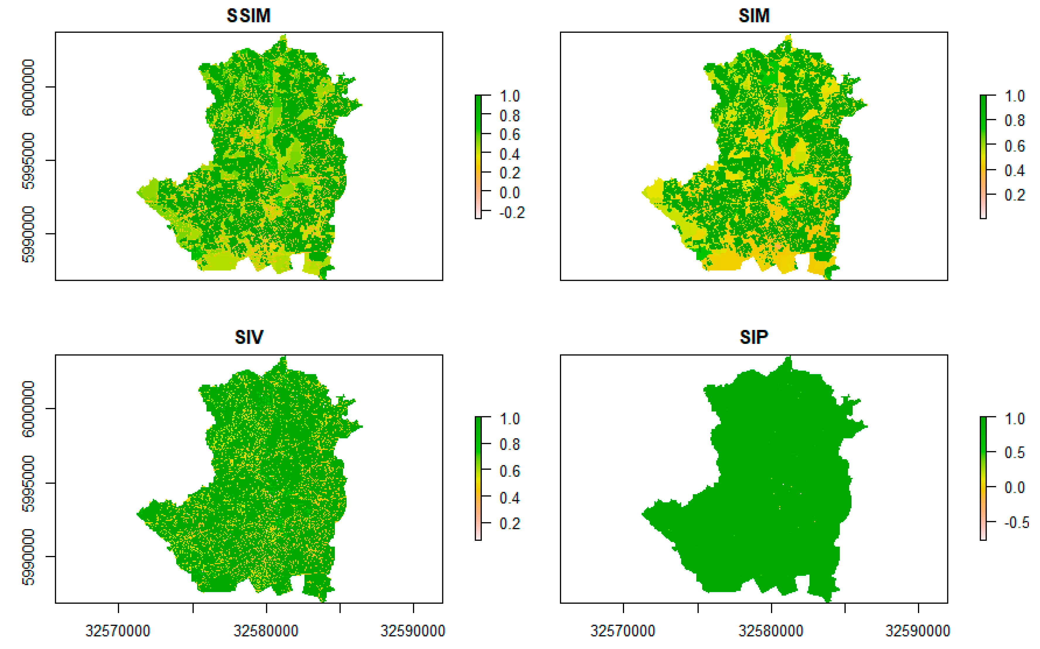
2.5. Statistical Maps Comparison

We first compared the maps resulting from the first and second assessments to evaluate the improvement in mapping precision. We then compared the maps resulting from the second and third assessments to estimate the mapping accuracy discrepancy. We used the structural similarity index (SSIM index) from Jones et al. [56] for visual interpretation and statistical analysis. This index provides three distinctive measures of spatial heterogeneity in map structures: similarity in means (SIM), similarity in variance (SIV) and similarity in pattern (SIP) of spatial covariance. SIM is the ratio of twice the product of the local means to their summed squares. It ranges from 0 to 1, in which 0 characterizes two maps for which means are dissimilar (in this case, different modelled ES local abundances), 1 if means are similar (similar modelled ES local abundances). The SIV is the ratio of twice the product of the local standard deviations to their summed variances. SIV ranges from 0 to 1, in which 0 is indicated if variances are dissimilar (ES are not similarly distributed), 1 if variances are similar (ES are similarly distributed). The SIP is the ratio of the local covariance to the product of the local standard deviation. It ranges between −1 and 1, in which −1 indicates a negative spatial correlation, 1 a positive spatial correlation and 0 indicates that the distributions are independent. The SSIM index compares output values of maps at pixel level and accounts for the values of neighboring pixels through a window of 3 × 3 pixels. The method allows for a spatially explicit difference analysis between two maps, including spatially explicit differences in means, variances and covariances, taking spatial dependencies between neighboring cells into account. All statistical analyses were conducted using the software R [57] and based on the script provided by Jones et al. [56].

3. Results

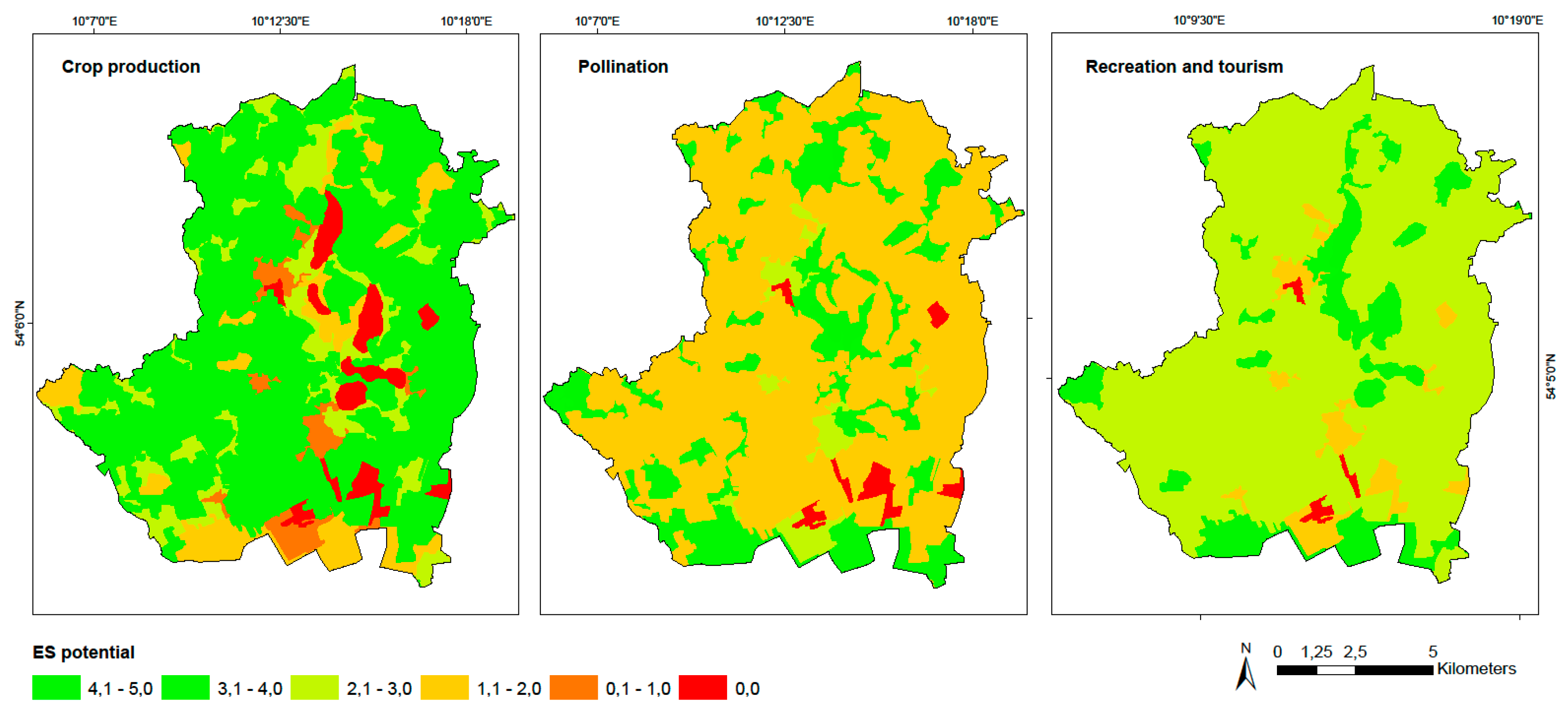
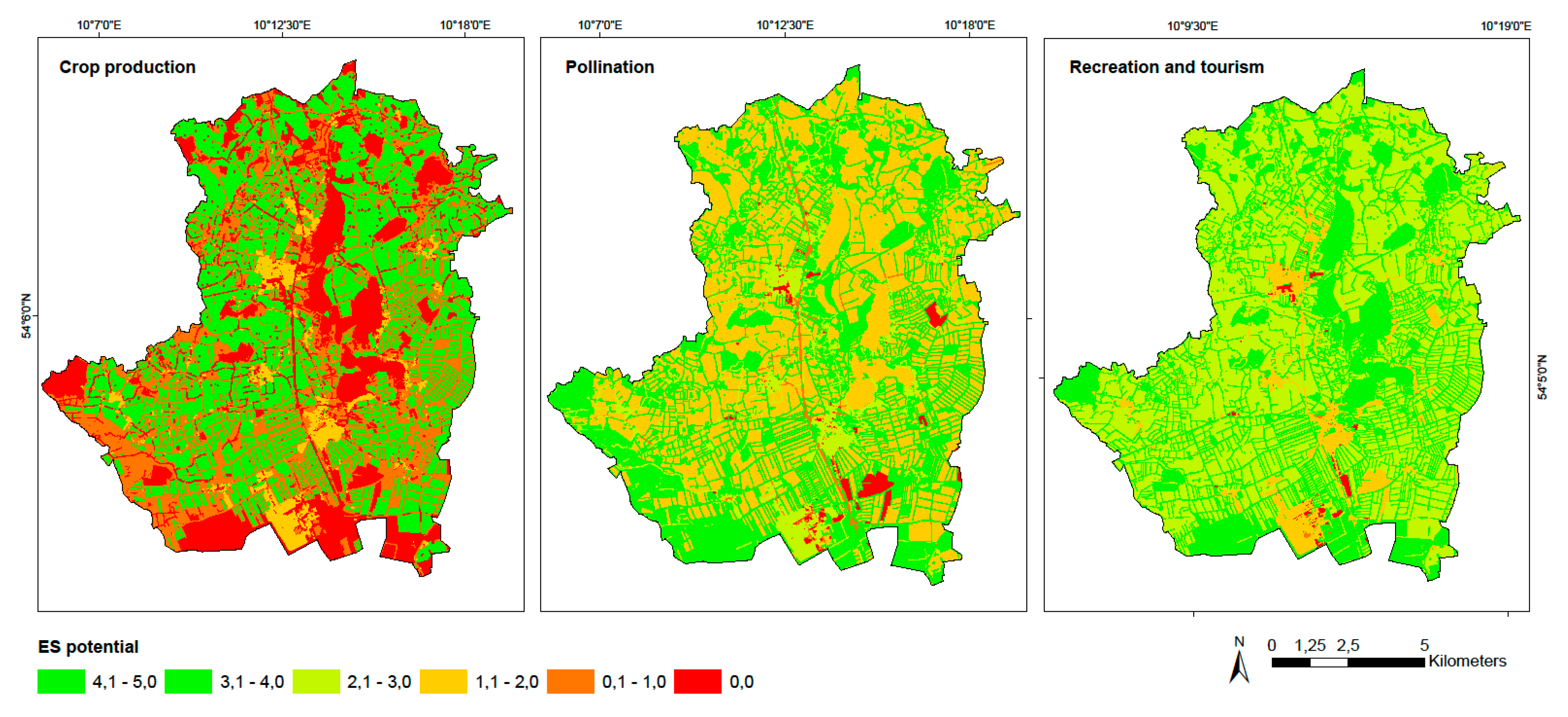
3.1. First Level Assessment

For the first level assessment, the ES potential supply was evaluated and mapped using the ES assessment matrix and CLC data. Figure 4 shows the spatial distribution of three ES potentials in the CSA: crop production, pollination and recreation and tourism services. A relative scale ranging from zero (no relevant capacity) to five (very high relevant capacity) was used. As the study area is mainly composed of “arable land” (see Table 1 for a description of land use classes share within the CSA), the maps show an overall high crop production potential, a low pollination potential and a moderate recreation and tourism potential for the area. High and very high pollination potentials are patchily distributed and correspond to “broad-leaved forest”, “coniferous forest”, “Pastures” and “land principally occupied by agriculture, with significant areas of natural vegetation”. High and very high recreation and tourism potentials correspond to “broad-leaved forest”, “coniferous forest” and “water bodies”.

3.2. Second Level Assessment

Figure 5 shows the spatial distribution of three ES in the CSA: crop production, pollination and recreation and tourism services. These maps are based on the ATKIS/InVeKoS datasets and show a more fragmented ES potential than the maps from the first level assessment, due to the inclusion of small habitats and landscape elements. Yet the resulting maps show the same global patterns (Figure 5): fewer areas sustain crop production, but have an overall high crop production potential, a low pollination potential and a moderate recreation and tourism potential.

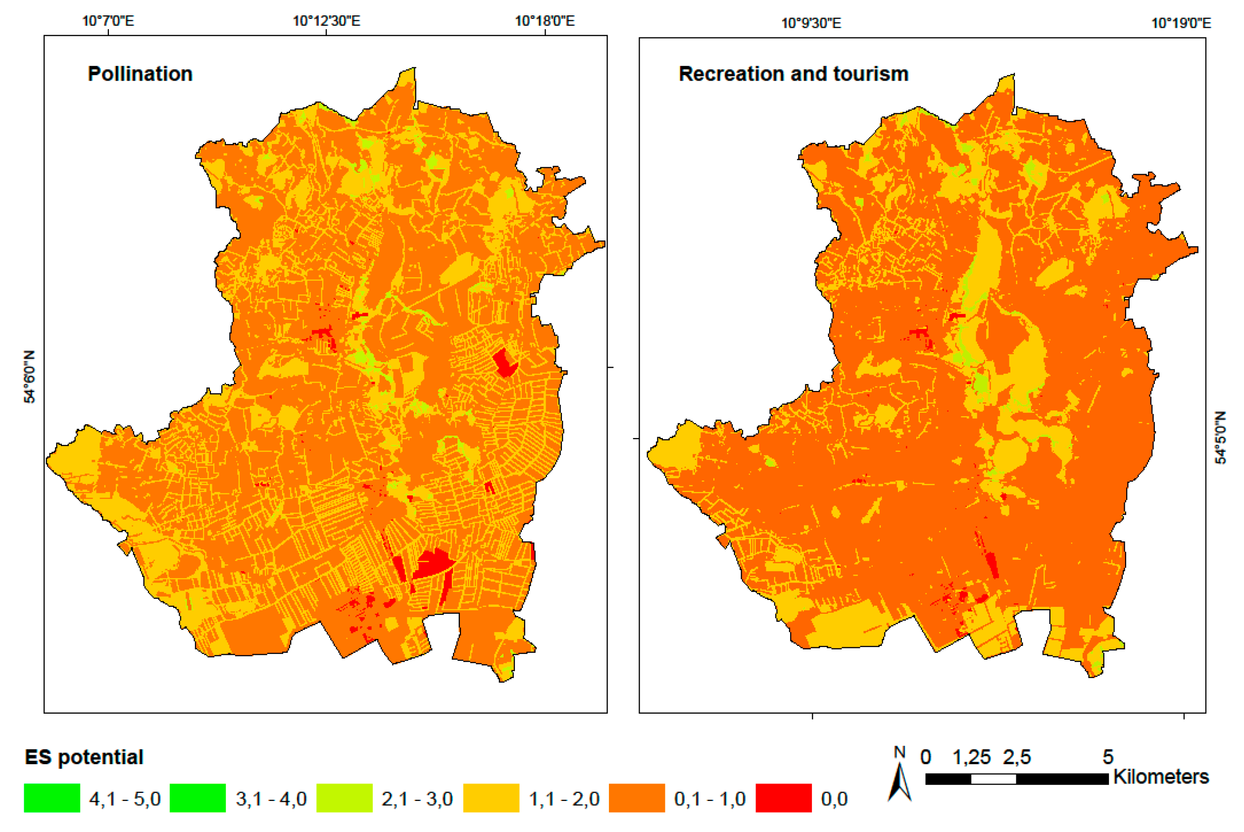
3.3. Third Level Assessment

The final ES potential maps (Figure 6) were obtained by combining the ecosystem condition index map (Figure S1 in the Supplementary Materials) and the ES potential maps from the second level of assessment. Only those ES which have a positive relationship with EC were included in this assessment (see Section 2.2.3), so for instance crop production was excluded. As none of the ecosystems in the CSA is in a very good condition (EC values are between 0.052 and 0.514, whereas the maximum achievable value is 1), the overall potentials of the CSA to supply ES are greatly reduced.

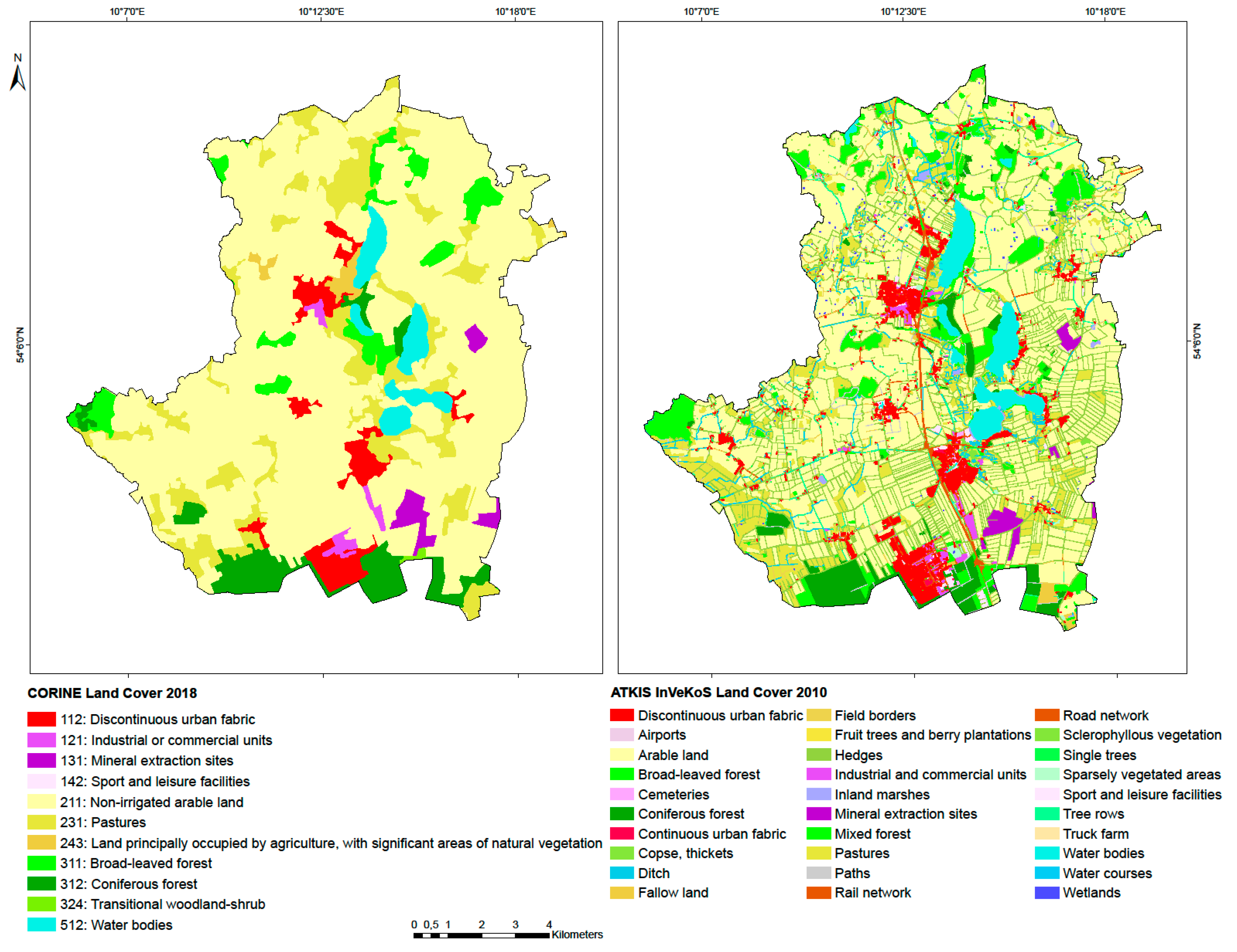
3.4. CORINE Land Cover and ATKIS/InVeKoS Typology Differences

Overall, there is a relatively high correspondence between the two datasets: around 70% of the CSA area is classified in the same LULC class in the two datasets. The main difference between CLC and ATKIS/InVeKoS datasets comes from the different resolutions for the LULC classes in both datasets, as LULC classes, which are mainly composed of large elements in the ATKIS/InVeKoS dataset, have a high matching level with CLC LULC classes: this is the case for “water bodies” (99%), “non-irrigated arable land” (81%), “industrial or commercial units” (64%) and “coniferous forest” (63%) classes. The LULC classes “discontinuous urban fabric”, “mineral extraction sites”, “pastures” and “broad-leaved forest” have however a matching level around 50% with a perfect correspondence for elements bigger than the CLC MMU.

There is a clear typology mismatch between the two datasets for the LULC classes that can be found only in the CLC dataset: The CLC LULC class “land principally occupied by agriculture, with significant areas of natural vegetation” mainly corresponds to arable land (27%) or pastures (42%) in the ATKIS/InVeKoS LULC classification, whereas “transitional woodland/shrub” is mainly classified as arable land (52%) or mixed forest (37%). Unlike the CLC classification, the ATKIS/InVeKoS dataset does not differentiate conventional arable land or pastures from agricultural land with natural areas. The ATKIS/InVeKoS classification considers “transitional woodland/shrub” areas as arable land or mixed forest, but does not consider afforestation/deforestation processes unlike the CLC classification (see Section 2.2.1 for a definition of CLC classes)

ES scores were recalculated for each CLC LULC class according to the percentage of each composing ATKIS/InVeKoS LULC class and their ES matrix scores (for instance, if the CLC LULC Class 1 was composed of 10% ATKIS/InVeKoS Class 1 (ES score 2) and 90% of the ATKIS/InVeKoS Class 2 (ES score 0), then the CLC LULC Class 1 has a ES score of 0.2 in the recalculated matrix). The ES scores from the original and the recalculated matrix were then compared. The LULC class “land principally occupied by agriculture, with significant areas of natural vegetation” showed a low variance between the ES scores from the initial matrix and the recalculated matrix (0.6 point) but showed a high variance for the CLC class “transitional woodlands, sclerophyllous vegetation” (1.6 point). This explains some variations in ES mapping, however only for a relatively small fraction of the CSA (the LULC classes “land principally occupied by agriculture, with significant areas of natural vegetation” and “transitional woodlands, sclerophyllous vegetation” represent less than 1% of the area).

For those LULC classes that were not included in the CLC dataset, the landscape elements correspond in the CLC map to the “non-irrigated arable land” (77%) and “pastures” (17%). This indicates that landscape elements are not considered in the CLC map, as they do not match the “land principally occupied by agriculture, with significant areas of natural vegetation” CLC LULC class. We can therefore assume that this LULC class is not integrated in the CLC map because the MMU is too coarse.

3.5. Statistical Comparison of First and Second Level Assessment

The resulting maps have similar ES potentials local abundance, variance and are highly correlated with a high to very high similarity in mean values (73.85 to 99.80% of the CSA has a SIM > 0.5), a high similarity in their variances (83.24 to 99.19% of the CSA has a SIV > 0.5) and a high positive spatial correlation (99.61 to 100% of the CSA has a SIP > 0) (Table S2 in the Supplementary Materials). Different patterns can be observed for the different ES and ES categories: the higher discrepancy between ES maps are for nutrient regulation, crop (Figure 7) and fiber productions, water purification and global climate regulation services, whereas minerals and fish provisioning have the lowest discrepancy. The differences between crop and fiber supply maps are mainly due to higher dissimilarity in local abundance, whereas the nutrient regulation maps differ in local abundance and variance. Cultural services tend to have a higher SIM than other services maps. Most of the regulation and maintenance services such as pollination, nutrient regulation and global climate regulation, but also cultural services and wild food production maps have a relatively lower SIV, whereas provisioning services are characterized by a high SIV (see Figure 7 for exemplary spatial agreement maps showing crop production services).

3.6. Statistical Comparison Second and Third Level Assessment

For most of the ES maps, the two mapping methods show highly different local ES potentials, however the variances and covariances have a low to a very high similarity in means (21.71 to 99.11% of the CSA has a SIM > 0.5), but very high similarity in variance (89.09 to 99.82% of the CSA has a SIV > 0.5) and an almost perfect spatial correlation (99.96 to 100% of the CSA has a SIP > 0) for all the ES (Table S3 in the Supplementary Materials). The correlation between the maps is to be expected as the map of the third level assessment is calculated based on the other map. We observe different patterns for each ES category: cultural services have the lowest SSIM values, followed by regulation services (except nutrient regulation) and provisioning services, which have the highest SSIMs. Overall, regulation and maintenance services tend to have a lower SIV than other ES categories (except for groundwater recharge and air quality regulation).

The spatial agreement between the maps depends on the number of ecosystems that deliver each ES, their sizes, the state of the ecosystem and the proportion of the area that potentially deliver each ES. ES that rely on few and in good condition LULC classes tend to have a higher SIM: fish provisioning has the higher SIM values and is sustained by few LULC classes (water bodies and water courses), which represent a small fraction of the CSA and tend to have a better ecological condition than other LULC classes. Nutrient regulation is supplied by a broader range of LULC types and has a high SIM (Figure 8). This may be due to the fact that this ES is mainly sustained by ecosystems that do not represent a high share of the total CSA (landscape elements and forests).

4. Discussion

4.1. Discrepancies in ES Maps Based on Different Spatial Resolutions

The results of the statistical map comparisons show that using coarse spatial resolution leads to a relatively small, but still nonnegligible differences. Most of the provisioning services and regulation and maintenance services maps are more affected by the spatial resolution than the cultural services maps. The differences in SSIM can be explained by the overestimation or underestimation of different ecosystems in the CLC dataset and by the capacity of these ecosystems to provide multiple or single ES. Arable lands mainly deliver one provisioning ES: crop production. Arable lands are overestimated in the CLC dataset, and increasing the spatial resolution reduces the total arable land area. Hence, the capacity of the CSA to produce crops diminishes in the second assessment. Landscape elements (such as hedgerows and field borders) can provide a wide range of ES, particularly maintenance and regulation services. Landscape elements only appear in high resolution LULC data; therefore, maintenance and regulation services are not appropriately mapped when using CLC as input data. As landscape elements are relatively small, the two mapping approaches using different LULC datasets still have a high similarity in variance. Cultural services are generated by more diverse LULC classes and are therefore relatively less affected by the spatial resolution.

For an ES assessment at the scale of the CSA, using CLC or more detailed LULC data would provide outputs with a low degree of structural differences, particularly for cultural services. There is however no unique appropriate resolution and our conclusions may be valid only for a similar scale of assessment. Kandziora et al. [26] showed for instance that the ATKIS/InVeKoS dataset was required for a reliable ES assessment of provisioning services at the plot scale. Similarly, Rioux et al. [58] showed that a spatial resolution of 5 m or finer is required to adequately map the ES provided by small greenspaces in urban areas. This would be especially true for highly fragmented landscapes, with a high share of linear elements and small habitats, which cannot be captured by coarse spatial resolution data such as CLC [59]. On the other hand, a high level of accuracy can be misleading when working at a larger scale and the results may not be serviceable for or understood by decision makers.

4.2. Discrepancies in ES Maps Based on Different Data Complexity

The results of the statistical map comparisons show that including ecosystem condition indicators in ES assessments has a high influence on the resulting maps for most of the ES, mainly because of the dissimilarities in mean values, however with a low variance discrepancy and a high spatial correlation. This suggests that LULC proxies, even with a high spatial resolution, do not sufficiently capture spatial heterogeneity in ES potential: for most of the considered ES potentials, local abundance would change considerably when accounting for ecosystem condition. These results concur with the studies by Eigenbrod et al. [25] and van der Biest et al. [22] who question the appropriateness of using LULC data as ES delivery proxies for different assessment scales and for different mapping purposes (but see Roche and Campagne [13] for contrasting results). LULC proxies are not appropriate for a local quantitative assessment i.e., to assess how much ES can be delivered at a specific location, under the assumption that it substantially depends on ecosystem condition. However, the high similarity in variances implies that the maps have similar spatial ES clusters and therefore that mapping ES hot spots and cold spots with the two different LULC datasets would obtain similar results.

4.3. Validation

We compared statistical maps to measure the degree of spatial conformity between comparable models with different spatial resolutions and data complexities. This does not constitute a measure of the overall accuracy of the assessment. Assessing model accuracy generally implies a validation using independent data such as primary data, which is generally feasible only for some provisioning services such as agricultural or timber productions [60], but see Sinclair et al. [61] and Chabert and Sarthou [62]. However, models adapted to a local context, with a higher spatial resolution or taking site-specific characteristics into account, generally provide a more precise assessment of ES processes, and their outputs are more reliable [63]. Moreover, if we assume that the capacity of an ecosystem to deliver ES depends on its condition, the results including EC indicators should be closer to the true distribution of ES potential.

4.4. Sources of Uncertainties of the Method

ES assessment at the landscape scale is subject to intrinsic uncertainties, which originate from the complexities of landscape and ecosystem processes. First, land cover classifications can imply uncertainties, mainly because of scale mismatches between landscape structure and the spatial data [21]. Even though the accuracy of spatial data has significantly increase with the development of remote sensing technologies, LULC classifications still contains landscape simplifications (as every map), generalizations or even misclassifications [64]. The use of higher spatial resolution data can help to reduce data uncertainties, so in this sense, the use of ATKIS/InVeKoS datasets is more reliable than the CLC dataset.

Second, uncertainties are inherent to the ES assessment field and our still insufficient knowledge on the relationships between ecosystems and ES supply [17,18,19]. For many ES, it is difficult to allocate ES delivery to specific LULC classes, above all for regulation and cultural services, as they are often provided by a combination of LULC with specific characteristics. Even if the importance of a good ecosystem condition for the delivery of ES is widely recognized [24,55,65], the effects of ecosystem condition parameters on ecosystem functioning and the basic mechanisms are still poorly understood [4,66]. van Oudenhoven et al. [67], Kandziora et al. [68], Balvanera et al. [18] and Harrison et al. [55] provide overviews of relationships between different EC/ES indicators and (some) ES, but they do not reach a consensus. Moreover, according to Braat and Brink [69] and Cardinale et al. [70], there may not be a linear relationship between biodiversity, EC and ES. As there is no clear and quantifiable information, it was not possible to adjust the importance of each indicator for each ES.

Lastly, the method entails uncertainties inherent to expert-based methods. Resulting ES assessments are strongly dependent on the level of knowledge of experts which can be subjective in scoring procedures [21]. For instance, less well-known ecosystems and non-directly used services may be underestimated by experts [14,71]. The number and selection of experts are critical and can reduce the level of uncertainty of the model [13,21]. The small size of the CSA considerably reduced the number of potentially relevant experts, as the task necessitates local knowledge on ecosystems and related ES.

4.5. Suggestions for Improvement

4.5.1. Data Availability

The feasibility of the different levels of assessment generally depends on the data availability for the study area. Among the data used in this study, only CLC and landscape fragmentation data are directly available and usable for all EU member states. Land cover datasets with a high resolution (covering for landscape elements) may or may not be available for other countries or regions. In Germany, this information can however not be accessed freely, due to data protection (InVeKoS) or commercial (ATKIS) reasons. For most of the ecosystem condition indicators recommended by the MES report, the needed data were not available for our CSA. Another issue is the scale for which the different indicators have been developed: most of them are not adapted to the local scale and their spatial resolutions do not allow for a local differentiation, and therefore spatially explicit assessment. Even if the availability of remote-sensing data has increased (e.g., Sentinel-2 based data products), data accessibility and availability is still a major issue for ES assessment. A typical example is data on ecosystem pressures such as the use of pesticides, fertilizers and biomass uptake that would greatly improve the index. The data should be made available and used in models to increase the accuracy of results.

4.5.2. Selecting Adapted Ecosystem Condition Indicators

The three ecosystem condition indicators used for this study were chosen because they were recommended in the fifth MAES report (see Maes et al. [35]). These indicators were developed to support national ecosystem assessments and were selected due to their spatial explicitness and sensitivity to change. Indicators that are suitable at the national scale may not necessarily be suitable for a sub-national or a local assessment: the spatial resolution may not be adaptable, and the indicators may be not sensitive to local land management and/or ecosystem condition changes. From the MAES list of recommended key indicators, we selected only relevant and complementary indicators, as a relatively large number of the indicators proposed in the report can be considered redundant and/or not adaptable to the local scale. The three ecosystem condition indicators selected for this study are still not completely independent and to some extent contain redundant information. For example, as biodiversity is usually positively affected by SOC values and negatively by landscape fragmentation, RLIs probably already include some information on the first two indicators. Despite their redundancy, the chosen indicators provide different information on ecosystem condition and their combination provides a relatively good estimation of the condition of different ecosystems. Another issue is that the different indicators are strongly linked to LULC: the different RLIs were calculated per ecosystem type and the SOC and fragmentation values are also largely a consequence of local land use. The outcomes of the second and third level assessments could have been more contradictory if the ecosystem condition indicators would have been measured differently, e.g., based on field data or if we had selected other ecosystem condition indicators.

5. Conclusions

Our study addresses some important issues in regard to ES assessments at a local level, where the quality of data is often critical. To our knowledge, this is one of the first studies to assess and map ES at the local scale based on ecosystem condition indicators recommended by the fifth MES report. In contrast to most of the previously published work, a broad range of ES was considered, and we compared the effects of different assessment methods on individual ES and on ES categories.

One of the main challenges for local ES assessments and mapping is finding and applying indicators, related quantification methods and data for comprehensible, reliable and feasible assessments. A reliable analysis should be as detailed as necessary and possible but is however often hampered by the lack of appropriate data for the quantification of each service. The context in which the assessment is implemented should guide the selection of the ES assessment methods and data. Yet a critical aspect for mapping accuracy is the capacity of the used model to capture spatial heterogeneity of ES potentials at the desired level. This paper compared three assessment methods that combine expert judgments, LULC data and ecosystem condition indicators in order to find the required resolution and data for an assessment in a local-scale case study.

Our results suggest that a high spatial resolution including landscape elements (such as hedgerows and field borders) does not drastically change the output of the spatial assessment at the local scale. However, by introducing LULC classes spatial variability, the use of EC indicators in the mapping can lead to different ES potential spatial patterns. This mainly depends on the number and characteristics of the chosen LULC classes, but also the landscape patterns of the studied area: map discrepancies tend to increase with the variety and size of LULC that are linked to ES in the matrix and the proportion of small elements in the studied area.

The results of this study show that expert-based methods combined with local data on ecosystem condition can be a feasible and efficient method for a local assessment of the capacity of a landscape to provide a wide range of ES. Nevertheless, the ES assessment method needs to be improved by exploring the different relationships between ES and the different EC indicators, but also by adding other essential ecosystem condition indicators and socioecological factors. Knowledge of the causal relationships between ES and ecosystem conditions needs to be better documented in different ecosystem types. This should also increase the accuracy of ES models.

References

1. Millennium Ecosystem Assessment. Ecosystems and Human Well-Being: Biodiversity Synthesis; World Resources Institute: Washington, DC, USA, 2005. [Google Scholar]
2. Maes, J.; Egoh, B.; Willemen, L.; Liquete, C.; Vihervaara, P.; Schägner, J.P.; Grizzetti, B.; Drakou, E.G.; La Notte, A.; Zulian, G.; et al. Mapping ecosystem services for policy support and decision making in the European Union. Ecosyst. Serv. 2012, 1, 31–39. [Google Scholar] [CrossRef]
3. Hansen, R.; Pauleit, S. From multifunctionality to multiple ecosystem services? A conceptual framework for multifunctionality in green infrastructure planning for urban areas. AMBIO 2014, 43, 516–529. [Google Scholar] [CrossRef] [PubMed] [Green Version]
4. De Groot, R.S.; Alkemade, R.; Braat, L.C.; Hein, L.; Willemen, L. Challenges in integrating the concept of ecosystem services and values in landscape planning, management and decision making. Ecol. Complex. 2010, 7, 260–272. [Google Scholar] [CrossRef]
5. Martínez-Harms, M.J.; Balvanera, P. Methods for mapping ecosystem service supply: A review. Int. J. Biodivers. Sci. Ecosyst. Serv. Manag. 2012, 8, 17–25. [Google Scholar] [CrossRef]
6. Grêt-Regamey, A.; Weibel, B.; Kienast, F.; Rabe, S.-E.; Zulian, G. A tiered approach for mapping ecosystem services. Ecosyst. Serv. 2015, 13, 16–27. [Google Scholar] [CrossRef]
7. Burkhard, B.; Kroll, F.; Müller, F. Landscapes’ capacities to provide ecosystem services—A concept for land-cover based assessments. Landsc. Online 2009, 15, 1–22. [Google Scholar] [CrossRef]
8. Burkhard, B.; Kroll, F.; Nedkov, S.; Müller, F. Mapping ecosystem service supply, demand and budgets. Ecol. Indic. 2012, 21, 17–29. [Google Scholar] [CrossRef]
9. Burkhard, B.; Kandziora, M.; Hou, Y.; Müller, F. Ecosystem service potentials, flows and demands–concepts for spatial localisation, indication and quantification. Landsc. Online 2014, 34, 1–32. [Google Scholar] [CrossRef]
10. Villamagna, A.M.; Angermeier, P.L.; Bennett, E.M. Capacity, pressure, demand, and flow: A conceptual framework for analyzing ecosystem service provision and delivery. Ecol. Complex. 2013, 15, 114–121. [Google Scholar] [CrossRef]
11. Weibel, B.; Rabe, S.-E.; Burkhard, B.; Grêt-Regamey, A. On the importance of a broad stakeholder network for developing a credible, salient and legitimate tiered approach for assessing ecosystem services. One Ecosyst. 2018, 3, e25470. [Google Scholar] [CrossRef]
12. Campagne, C.S.; Roche, P.K. May the matrix be with you! Guidelines for the application of expert-based matrix approach for ecosystem services assessment and mapping. One Ecosyst. 2017, 3, e24134. [Google Scholar] [CrossRef]
13. Campagne, C.S.; Roche, P.; Müller, F.; Burkhard, B. Ten years of ecosystem services matrix: Review of a (r)evolution. One Ecosyst. 2020, 5, 106. [Google Scholar] [CrossRef]
14. Jacobs, S.; Burkhard, B.; van Daele, T.; Staes, J.; Schneiders, A. ‘The Matrix Reloaded’: A review of expert knowledge use for mapping ecosystem services. Ecol. Model. 2015, 295, 21–30. [Google Scholar] [CrossRef]
15. EEA. Corine Land Cover (CLC) 2018, Version 20b2. Available online: https://land.copernicus.eu/pan-european/corine-land-cover/clc2018 (accessed on 10 February 2020).
16. Schröter, M.; Remme, R.P.; Sumarga, E.; Barton, D.N.; Hein, L. Lessons learned for spatial modelling of ecosystem services in support of ecosystem accounting. Ecosyst. Serv. 2015, 13, 64–69. [Google Scholar] [CrossRef]
17. Bastian, O.; Haase, D.; Grunewald, K. Ecosystem properties, potentials and services–The EPPS conceptual framework and an urban application example. Ecol. Indic. 2012, 21, 7–16. [Google Scholar] [CrossRef]
18. Balvanera, P.; Siddique, I.; Dee, L.; Paquette, A.; Isbell, F.; Gonzalez, A.; Byrnes, J.E.K.; O’Connor, M.I.; Hungate, B.A.; Griffin, J.N. Linking Biodiversity and Ecosystem Services: Current Uncertainties and the Necessary Next Steps. BioScience 2014, 64, 49–57. [Google Scholar] [CrossRef]
19. Rendon, P.; Erhard, M.; Maes, J.; Burkhard, B. Analysis of trends in mapping and assessment of ecosystem condition in Europe. Ecosyst. People 2019, 15, 156–172. [Google Scholar] [CrossRef] [Green Version]
20. Eigenbrod, F.; Armsworth, P.R.; Anderson, B.J.; Heinemeyer, A.; Gillings, S.; Roy, D.B.; Thomas, C.D.; Gaston, K.J. Error propagation associated with benefits transfer-based mapping of ecosystem services. Biol. Conserv. 2010, 143, 2487–2493. [Google Scholar] [CrossRef]
21. Hou, Y.; Burkhard, B.; Müller, F. Uncertainties in landscape analysis and ecosystem service assessment. J. Environ. Manag. 2013, 127, 117–131. [Google Scholar] [CrossRef]
22. van der Biest, K.; Vrebos, D.; Staes, J.; Boerema, A.; Bodí, M.B.; Fransen, E.; Meire, P. Evaluation of the accuracy of land-use based ecosystem service assessments for different thematic resolutions. J. Environ. Manag. 2015, 156, 41–51. [Google Scholar] [CrossRef]
23. Schwartz, M.W.; Brigham, C.A.; Hoeksema, J.D.; Lyons, K.G.; Mills, M.H.; van Mantgem, P.J. Linking biodiversity to ecosystem function: Implications for conservation ecology. Oecologia 2000, 122, 297–305. [Google Scholar] [CrossRef] [PubMed]
24. Haines-Young, R.H.; Potschin, M. The links between biodiversity, ecosystem services and human well-being. Ecosyst. Ecol. New Synth. 2010, 1, 110–139. [Google Scholar]
25. Eigenbrod, F.; Armsworth, P.R.; Anderson, B.J.; Heinemeyer, A.; Gillings, S.; Roy, D.B.; Thomas, C.D.; Gaston, K.J. The impact of proxy-based methods on mapping the distribution of ecosystem services. J. Appl. Ecol. 2010, 47, 377–385. [Google Scholar] [CrossRef]
26. Kandziora, M.; Burkhard, B.; Müller, F. Mapping provisioning ecosystem services at the local scale using data of varying spatial and temporal resolution. Ecosyst. Serv. 2013, 4, 47–59. [Google Scholar] [CrossRef]
27. Ecosystem Organization of a Complex Landscape. Long-Term Research in the Bornhöved Lake District, Germany; Fränzle, O., Blume, H.-P., Dierssen, K., Kappen, L., Eds.; Springer: Berlin/Heidelberg, Germany, 2008; ISBN 978-3-540-75811-2. [Google Scholar]
28. Bicking, S.; Burkhard, B.; Kruse, M.; Müller, F. Mapping of nutrient regulating ecosystem service supply and demand on different scales in Schleswig-Holstein, Germany. One Ecosyst. 2018, 3, e22509. [Google Scholar] [CrossRef] [Green Version]
29. Bach, M.; Breuer, L.; Frede, H.-G.; Huisman, J.A.; Otte, A.; Waldhardt, R. Accuracy and congruency of three different digital land-use maps. Landsc. Urban Plan. 2006, 78, 289–299. [Google Scholar] [CrossRef]
30. Burkhard, B.; Maes, J. 5.1. What to map? In Mapping Ecosystem Services; Syrbe, R.-U., Schröter, M., Grunewald, K., Walz, U., Burkhard, B., Eds.; Pensoft Publisher: Sofia, Bulgaria, 2017. [Google Scholar]
31. Burkhard, B.; Maes, J. Mapping Ecosystem Services; Pensoft Publishers: Sofia, Bulgaria, 2017; ISBN 978-954-642-829-5. [Google Scholar]
32. Haines-Young, R.; Potschin, M. Common International Classification of Ecosystem Services (CICES), Version 5.1. Guidance on the Application of the Revised Structure. 2018. Available online: https://cices.eu/content/uploads/sites/8/2018/01/Guidance-V51-01012018.pdf (accessed on 10 January 2020).
33. Müller, F.; Bicking, S.; Ahrendt, K.; Bac, D.K.; Blindow, I.; Fürst, C.; Haase, P.; Kruse, M.; Kruse, T.; Ma, L. Assessing ecosystem service potentials to evaluate terrestrial, coastal and marine ecosystem types in Northern Germany–An expert-based matrix approach. Ecol. Indic. 2020, 112, 106116. [Google Scholar] [CrossRef]
34. European Commission. Our Life Insurance, Our Natural Capital: An EU Biodiversity Strategy to 2020; European Commission: Belgium, Brussels, 2011; p. 244. [Google Scholar]
35. Maes, J.; Teller, A.; Erhard, M.; Grizzetti, B.; Barredo, J.I.; Paracchini, M.; Condé, S.; Somma, F.; Orgiazzi, A.; Jones, A.; et al. Mapping and Assessment of Ecosystems and their Services: An Analytical Framework for Ecosystem Condition; Publications Office of the European Union: Luxembourg, 2018. [Google Scholar]
36. EEA. Landscape Fragmentation in Europe. Joint EEA-FOEN Report. Literaturverz. S.69–76; European Environment Agency: Copenhagen, Denmark, 2011; ISBN 978-92-9213-215-6. [Google Scholar]
37. Fahrig, L.; Rytwinski, T. Effects of roads on animal abundance: An empirical review and synthesis. Ecol. Soc. 2009, 14, 21. [Google Scholar] [CrossRef]
38. Mitchell, M.G.E.; Suarez-Castro, A.F.; Martinez-Harms, M.; Maron, M.; McAlpine, C.; Gaston, K.J.; Johansen, K.; Rhodes, J.R. Reframing landscape fragmentation’s effects on ecosystem services. Trends Ecol. Evol. 2015, 30, 190–198. [Google Scholar] [CrossRef] [Green Version]
39. Vié, J.-C.; Hilton-Taylor, C.; Pollock, C.; Ragle, J.; Smart, J.; Stuart, S.N.; Tong, R. The IUCN Red List: A Key Conservation Tool. Wildlife in a Changing World–An Analysis of the 2008 IUCN Red List of Threatened Species; IUC: Gland, Switzerland, 2009; p. 1. [Google Scholar]
40. Butchart, S.H.M.; Akçakaya, H.R.; Chanson, J.; Baillie, J.E.M.; Collen, B.; Quader, S.; Turner, W.R.; Amin, R.; Stuart, S.N.; Hilton-Taylor, C. Improvements to the red list index. PLoS ONE 2007, 2, e140. [Google Scholar] [CrossRef]
41. Klinge, A. Die Amphibien und Reptilien Schleswig-Holsteins-Rote Liste, 3. Fassung, Dezember 2003; LANU: Flintbek, Germany, 2003; ISBN 3-923339-93-3. [Google Scholar]
42. Knief, W.; Berndt, R.K.; Hälterlein, B.; Jeromin, K.; Kieckbucsh, J.J.; Koop, B. Die Brutvögel Schleswig-Holsteins-Rote Liste, 5. Fassung-Oktober 2010; LANU: Flintbek, Germany, 2010; ISBN 3-937937-45-8. [Google Scholar]
43. Borkenhagen, P.; Drews, A. Die Säugetiere Schleswig-Holsteins-Rote Liste, 4. Fassung, (Datenstand: November 2013); Ministerium für Energiewende Landwirtschaft Umwelt und Ländliche Räume des Landes Schleswig-Holstein (MELUR): Kiel, Germany, 2014; ISBN 978-3-937937-76-2.
44. Juslén, A.; Pykälä, J.; Kuusela, S.; Kaila, L.; Kullberg, J.; Mattila, J.; Muona, J.; Saari, S.; Cardoso, P. Application of the Red List Index as an indicator of habitat change. Biodivers. Conserv. 2016, 25, 569–585. [Google Scholar] [CrossRef] [Green Version]
45. Daily, G.C. Nature’s services. In Societal Dependence on Natural Ecosystems; Island Press: Washington, DC, USA, 1997; ISBN 1-55963-475-8. [Google Scholar]
46. Swinton, S.M.; Lupi, F.; Robertson, G.P.; Landis, D.A. Ecosystem Services from Agriculture: Looking Beyond the Usual Suspects. Am. J. Agric. Econ. 2006, 88, 1160–1166. [Google Scholar] [CrossRef]
47. Hewitt, A.; Dominati, E.; Webb, T.; Cuthill, T. Soil natural capital quantification by the stock adequacy method. Geoderma 2015, 241, 107–114. [Google Scholar] [CrossRef] [Green Version]
48. Adhikari, K.; Hartemink, A.E. Linking soils to ecosystem services—A global review. Geoderma 2016, 262, 101–111. [Google Scholar] [CrossRef]
49. Drobnik, T.; Greiner, L.; Keller, A.; Grêt-Regamey, A. Soil quality indicators – From soil functions to ecosystem services. Ecol. Indic. 2018, 94, 151–169. [Google Scholar] [CrossRef]
50. Baveye, P.C.; Baveye, J.; Gowdy, J. Soil “Ecosystem” services and natural capital: Critical appraisal of research on uncertain ground. Front. Environ. Sci. 2016, 4, 609. [Google Scholar] [CrossRef]
51. Düwel, O.; Siebner, C.S.; Utermann, J.; Krone, F. Gehalte an Organischer Substanz in Oberböden Deutschlands Bericht über länderübergreifende Auswertungen von Punktinformationen im FISBo BGR; Bundesanstalt für Geowissenschaften und Rohstoffe: Hannover, Germany, 2007. [Google Scholar]
52. Mordhorst, A.; Fleige, H.; Zimmermann, I.; Burbaum, B.; Filipinski, M.; Cordsen, E.; Horn, R. Organische Kohlenstoffvorräte von Bodentypen in den Hauptnaturräumen Schleswig-Holsteins (Norddeutschland). Die Bodenkult. J. Land Manag. Food Environ. 2018, 69, 85–95. [Google Scholar] [CrossRef] [Green Version]
53. Spangenberg, J.H.; Görg, C.; Truong, D.T.; Tekken, V.; Bustamante, J.V.; Settele, J. Provision of ecosystem services is determined by human agency, not ecosystem functions. four case studies. Int. J. Biodivers. Sci. Ecosyst. Serv. Manag. 2014, 10, 40–53. [Google Scholar] [CrossRef] [Green Version]
54. Balvanera, P.; Pfisterer, A.B.; Buchmann, N.; He, J.-S.; Nakashizuka, T.; Raffaelli, D.; Schmid, B. Quantifying the evidence for biodiversity effects on ecosystem functioning and services. Ecol. Lett. 2006, 9, 1146–1156. [Google Scholar] [CrossRef] [Green Version]
55. Harrison, P.A.; Berry, P.M.; Simpson, G.; Haslett, J.R.; Blicharska, M.; Bucur, M.; Dunford, R.; Egoh, B.; Garcia-Llorente, M.; Geamănă, N. Linkages between biodiversity attributes and ecosystem services: A systematic review. Ecosyst. Serv. 2014, 9, 191–203. [Google Scholar] [CrossRef] [Green Version]
56. Jones, E.L.; Rendell, L.; Pirotta, E.; Long, J.A. Novel application of a quantitative spatial comparison tool to species distribution data. Ecol. Indic. 2016, 70, 67–76. [Google Scholar] [CrossRef]
57. R Core Team. A Language and Environment for Statistical Computing; R Foundation for Statistical Computing: Vienna, Austria, 2017. [Google Scholar]
58. Rioux, J.-F.; Cimon-Morin, J.; Pellerin, S.; Alard, D.; Poulin, M. How land cover spatial resolution affects mapping of urban ecosystem service flows. Front. Environ. Sci. 2019, 7, 345. [Google Scholar] [CrossRef]
59. Schulp, C.J.E.; Alkemade, R. Consequences of uncertainty in global-scale land cover maps for mapping ecosystem functions: An analysis of pollination efficiency. Remote Sens. 2011, 3, 2057–2075. [Google Scholar] [CrossRef] [Green Version]
60. Lavorel, S.; Bayer, A.; Bondeau, A.; Lautenbach, S.; Ruiz-Frau, A.; Schulp, N.; Seppelt, R.; Verburg, P.; van Teeffelen, A.; Vannier, C.; et al. Pathways to bridge the biophysical realism gap in ecosystem services mapping approaches. Ecol. Indic. 2017, 74, 241–260. [Google Scholar] [CrossRef] [Green Version]
61. Sinclair, M.; Mayer, M.; Woltering, M.; Ghermandi, A. Using social media to estimate visitor provenance and patterns of recreation in Germany’s national parks. J. Environ. Manag. 2020, 263, 110418. [Google Scholar] [CrossRef]
62. Chabert, A.; Sarthou, J.-P. Conservation agriculture as a promising trade-off between conventional and organic agriculture in bundling ecosystem services. Agric. Ecosyst. Environ. 2020, 292, 106815. [Google Scholar] [CrossRef]
63. Zulian, G.; Stange, E.; Woods, H.; Carvalho, L.; Dick, J.; Andrews, C.; Baró, F.; Vizcaino, P.; Barton, D.N.; Nowel, M.; et al. Practical application of spatial ecosystem service models to aid decision support. Ecosyst. Serv. 2018, 29, 465–480. [Google Scholar] [CrossRef]
64. Schulp, C.J.E.; Burkhard, B.; Maes, J.; van Vliet, J.; Verburg, P.H. Uncertainties in ecosystem service maps: A comparison on the European scale. PLoS ONE 2014, 9, e109643. [Google Scholar] [CrossRef] [Green Version]
65. Díaz, S.; Fargione, J.; Chapin, F.S.; Tilman, D. Biodiversity loss threatens human well-being. PLoS Biol. 2006, 4, e277. [Google Scholar] [CrossRef] [Green Version]
66. de Groot, R.S. Integrating the ecological and economic dimensions in biodiversity and ecosystem service valuation. In The Economics of Ecosystems and Biodiversity: The Ecological and Economic Foundations; TEEB: London, UK, 2010; Volume 40, pp. 10–15. [Google Scholar] [CrossRef]
67. van Oudenhoven, A.P.E.; Petz, K.; Alkemade, R.; Hein, L.; de Groot, R.S. Framework for systematic indicator selection to assess effects of land management on ecosystem services. Ecol. Indic. 2012, 21, 110–122. [Google Scholar] [CrossRef]
68. Kandziora, M.; Burkhard, B.; Müller, F. Interactions of ecosystem properties, ecosystem integrity and ecosystem service indicators—A theoretical matrix exercise. Ecol. Indic. 2013, 28, 54–78. [Google Scholar] [CrossRef]
69. Braat, L.C.; Brink, P. The Cost of Policy Inaction. The Case of Not Meeting the 2010 Biodiversity Target; Report to the European Commission under Contract: Brussels, Belgium, 2008. [Google Scholar]
70. Cardinale, B.J.; Duffy, J.E.; Gonzalez, A.; Hooper, D.U.; Perrings, C.; Venail, P.; Narwani, A.; Mace, G.M.; Tilman, D.; Wardle, D.A.; et al. Biodiversity loss and its impact on humanity. Nature 2012, 486, 59–67. [Google Scholar] [CrossRef] [PubMed]
71. Roche, P.K.; Campagne, C.S. Are expert-based ecosystem services scores related to biophysical quantitative estimates? Ecol. Indic. 2019, 106, 105421. [Google Scholar] [CrossRef]
Figure 1. Location of the study area in northern Germany (on the right) and distribution of administrative districts and Corine land-cover classes (CLC2018) (on the left).
Land 09 00348 g001
Figure 2. Working flow chart.
Land 09 00348 g002
Figure 3. Distribution of CORINE land cover data (CLC) (Level 1, 2018) and ATKIS/InVeKoS (Level 2, 2010) land cover classes in the study area Bornhöved. Agriculture represents 81.2% (CLC) or 72.4% (ATKIS/InVeKoS) of the total area, from which 67.2% (CLC) or 60.6% (ATKIS/InVeKoS) is dedicated to arable land. Forests covers only 9.2% (CLC) or 10.7% (ATKIS/InVeKoS) of the case study area. 6.4 (CLC) to 3.8% (ATKIS/InVeKoS) of the area is covered by artificial surfaces. In the CLC datasets, 0.1% of the area is covered by transitional woodland-shrub which has no equivalent in the other dataset. Landscape elements represent 2.9% of the total area in the ATKIS/InVeKoS datasets.
Land 09 00348 g003
Figure 4. Examples of three ecosystem services (ES) potential maps (crop production, pollination and recreation and tourism) using CLC land cover data and the ES potential matrix. 0.0: no potential, 0.1–1.0: very low potential, 1.1–2.0: low potential, 2.1–3.0: moderate potential, 3.1–4.0: high potential, 4.1–5.0: very high potential.
Land 09 00348 g004
Figure 5. Examples of three ES potential maps (crop production, pollination and recreation and tourism) using ATKIS and InVeKoS land cover data and the ES potential matrix. 0.0: no potential, 0.1–1.0: very low potential, 1.1–2.0: low potential, 2.1–3.0: moderate potential, 3.1–4.0: high potential, 4.1–5.0: very high potential.
Land 09 00348 g005
Figure 6. Examples of two ES potential maps (pollination and recreation and tourism) using ATKIS and InVeKoS land cover data, the ES potential matrix and ecosystem condition indicators. 0.0: no potential; 0.1–1.0: very low potential; 1.1–2.0: low potential; 2.1–3.0: moderate potential; 3.1–4.0: high potential; 4.1–5.0: very high potential.
Land 09 00348 g006
Figure 7. Map comparison between the crop production service potential with CLC and ATKIS/InVeKoS datasets. SSIM—structural similarity Index; SIM—similarity in means; SIV—similarity in variance; SIP—similarity in pattern of spatial covariance.
Land 09 00348 g007
Figure 8. Map comparison between the nutrient regulation service potential with only LULC data and LULC combines with EC indicators. SSIM—structural similarity index; SIM—similarity in means; SIV—similarity in variance; SIP—similarity in pattern of spatial covariance.
Land 09 00348 g008