Article

Planning for Dynamic Connectivity: Operationalizing Robust Decision-Making and Prioritization Across Landscapes Experiencing Climate and Land-Use Change

1
Biology Department, San Diego State University, 5500 Campanile Drive, San Diego, CA 92182-4614, USA
2
Institute for Ecological Monitoring and Management, San Diego State University, San Diego, CA 92182-4614, USA
3
Institute for Health Metrics and Evaluation, University of Washington, Seattle, WA 98195, USA
4
Point Blue Conservation Science, Petaluma, CA 94954, USA
*
Author to whom correspondence should be addressed.
Land 2020, 9(10), 341; https://doi.org/10.3390/land9100341
Submission received: 1 August 2020 / Revised: 11 September 2020 / Accepted: 19 September 2020 / Published: 23 September 2020
(This article belongs to the Special Issue Dynamic Landscape Connectivity)

Abstract

:
Preserving landscape connectivity is one of the most frequently recommended strategies to address the synergistic threats of climate change, habitat fragmentation, and intensifying disturbances. Although assessments to develop plans for linked and connected landscapes in response to climate and land-use change have been increasingly employed in the last decade, efforts to operationalize and implement these plans have been limited. Here, we present a framework using existing, available biological data to design an implementable, comprehensive multispecies connectivity plan. This framework uses a scenario-based approach to consider how ecosystems, habitats, and species may need to adapt to future conditions with an ensemble of connectivity models. We use the south coast ecoregion of California as an example to evaluate and prioritize linkages by combining linked metapopulation models and key landscape features (e.g., conservation planning status and implementation feasibility) to identify and prioritize a multispecies linkage network. Our analyses identified approximately 30,000 km2 of land, roughly one-fifth of our study area, where actions to preserve or enhance connectivity may support climate adaptation, nearly half of which is already conserved. By developing and implementing a dynamic connectivity assessment with an eye towards projected changes, our analysis demonstrates how dynamic connectivity can be integrated into feasible regional conservation and management plans that account for demographic as well as landscape change. We observed overlap across multiple models, reinforcing the importance of areas that appeared across methods. We also identified unique areas important for connectivity captured by our complementary models. By integrating multiple approaches, the resultant linkage network is robust, building on the strengths of a variety of methods to identify model consensus and reduce uncertainty. By linking quantitative connectivity metrics with prioritized areas for conservation, our approach supports transparent and robust decision-making for landscape planning, despite uncertainties of climate and land-use change.

Graphical Abstract

1. Introduction

Climate change is expected to result in rising temperatures, increased variability in precipitation, and more frequent disturbance events such as wildfire and floods [1]. The potential effects of these changing environmental conditions on wildlife may include latitudinal and elevational shifts in species’ ranges toward cooler climates [2], shifts in habitat elements such as vegetation type and cover, and changes in water availability, all with compounding impacts on food webs and natural communities. Maintaining biodiversity and ecological function in the face of the direct and indirect impacts of climate change is one of the central and burgeoning issues facing conservation planners. However, the primary threats to species’ capacity to adapt to these climate impacts are concurrent habitat fragmentation and loss caused by anthropogenic development and land-use changes that can result in barriers to dispersal [3]. With unprecedented climate-driven species extinctions predicted at the global and local levels [1], maintaining genetic diversity to support adaptation and landscape connectivity to allow for range shifts or migration are two of the most viable mechanisms for species to respond to the changing climate. Preserving landscape connectivity is therefore one of the most frequently recommended strategies to address these synergistic threats of climate change [4,5] habitat fragmentation [6], and increased disturbances [7,8].
Landscape connectivity can provide for dispersal, recolonization or immigration supporting small populations [9], and gene flow, particularly in patchy or fragmented habitats [10]. In response to the widespread habitat loss and fragmentation that has affected biodiversity and connectivity worldwide, conservation efforts have focused on establishing landscape-scale plans to delineate connected networks of core habitat. Traditionally, connectivity planning and implementation for these protected area networks have assumed static landscape conditions, primarily due to limitations in data availability and computational power. However, connectivity across these protected area networks will likely shift over time in response to landscape changes caused by changing climate and altered disturbance regimes [4,11].
Over the last 10–15 years, a range of analytical approaches and design strategies for climate-wise connectivity in dynamic landscapes have emerged, including many designed explicitly for conservation planning purposes [5]. Yet, it is unclear whether plans that explicitly include climate change have been incorporated into conservation actions [12], particularly for preserve networks that were established prior to the emergence of these new approaches. In locations that face the more proximate threats of habitat loss and fragmentation from increasing urbanization, connectivity planning and implementation often focus proactively on areas that are most constrained, or reactively on opportunistic investments to preserve connectivity. The uncertainty of planning for future conditions creates further challenges that may delay actions to preserve connectivity for climate adaptation [13]. However, integrating near-term barriers and challenges to connectivity plans as well as long-term resilience of the network given projected changes will likely yield greater conservation successes [14].
Assessments of climate-wise connectivity often rely on a focal species approach to identify linkages that will support movement and metapopulation persistence [5]. A multispecies framework for such assessments may confer a number of advantages [15,16,17]. Modeling connectivity for multiple species can capture different habitat associations, movement behaviors, and dispersal abilities and under scenarios of climate change, can reflect a range of projected responses. Emerging strategies that combine these species-based approaches to model functional connectivity with assessments of key structural features of the landscape to support connectivity have thus far proven to be the most effective for addressing both near-term and long-term threats [18,19]. Still, there is a need to further develop modeling approaches and long-range planning to simultaneously account for continued anthropogenic development and accommodate adaptation to climate change [20].
Planning for landscape connectivity under the synergistic effects of climate and land-use changes can be further strengthened with innovative methods that incorporate demographic constraints to species persistence. Spatially connected populations, or metapopulations, are formed as populations reorganize when there are large fluctuations in births and deaths across the landscape [21]. Reorganization can also follow when populations recolonize an area following disturbances (e.g., fire, drought, disease) that reduce populations in good habitat, fragment when contiguous habitat is split, or consolidate when new habitat forms [22]. Because of these processes, which are all likely to occur more frequently in the face of climatic and land-use shifts, population dynamics are integrally linked to connectivity. Although corridors or linkages are recognized as important to population persistence, the role of population dynamics in connectivity planning is not often assessed (but see [23]).
Efforts to develop proactive, adaptive planning for linked and connected landscapes under climate and land-use change have been increasingly employed [24,25]. However, there are still gaps in the operationalization and implementation of dynamic connectivity plans, likely because strategies must address uncertainty in future conditions, incorporate demographic constraints to species’ persistence, and account for other factors affecting the feasibility of actions to preserve connectivity and meet conservation objectives. One region with a history of rapid land-use development that is expected to continue is southern California, where high human population density and growth is correlated with increasing numbers of rare and threatened plants and animals [26] and increasing fire frequency [27]. Here, we present a scenario-based, multispecies approach to assess current and projected future connectivity with an ensemble of modeling methods to develop a multispecies linkage network for a southern California landscape. We evaluate and prioritize linkages to support structural and functional connectivity, combining the results of linked metapopulation models with connectivity and landscape metrics, conservation feasibility, and a climate assessment based on consensus from multiple climate scenarios. Our goal was to develop a framework to address the synergistic threats of climate and land-use change by integrating interrelated factors representing the biological value, climate value, and conservation considerations to support connectivity prioritization, planning, and implementation in a dynamic landscape. Our framework employs empirical data to assess and plan for likely landscape changes that will affect habitat suitability and population persistence, capturing both species pattern and population process responses. Using empirical data to account for demographic and landscape changes from climate scenarios, our findings highlight how dynamic connectivity approaches can account for uncertainty and support proactive and climate-resilient landscape conservation, management, and planning.

2. Materials and Methods
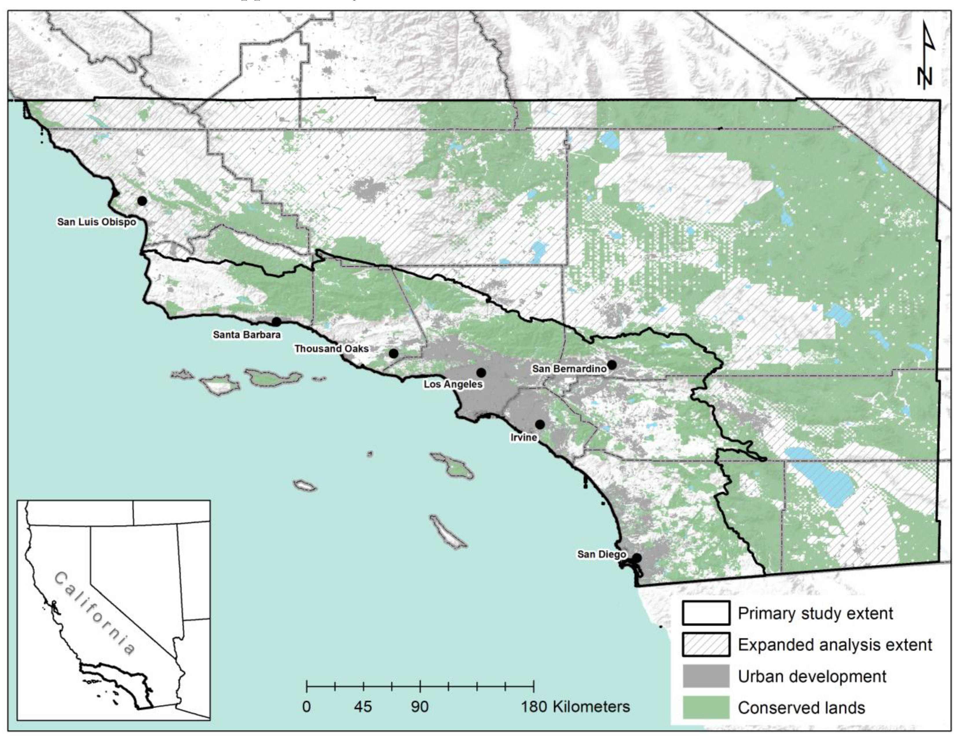
2.1. Study Area

This study focuses on the south coast ecoregion of southern California (Figure 1) from the Transverse and Peninsular mountains ranging from Santa Barbara County to the U.S. border with Mexico in San Diego County. To ensure we were capturing a range of climatic conditions and avoiding artifacts of edge effects in our connectivity modeling, we expanded our analytical extent north to the central coast and southern Sierra Nevada and incorporated desert regions to the east, encompassing lands within Monterey, Kings, Tulare, San Luis Obispo, Kern, San Bernardino, Santa Barbara, Ventura, Los Angeles, Orange, Riverside, San Diego, and Imperial Counties. Elevation in this area ranges from below sea level in the eastern deserts to 3506 m at the top of San Gorgonio Mountain in San Bernardino County. The Mediterranean climate of the study region is characterized by hot, dry summers and mild, wet winters with annual precipitation often less than 300 mm, virtually all coming during the winter months. Both precipitation and temperature vary across the study area, and are dependent on distance from the coast, elevation, and local topographic features. Temperatures ranges from averages of 14.8–31.9 °C in summer to averages of 0–14.2 °C in winter.

2.2. Modeling Approach

To address uncertainty in climatic projections and species’ responses to those changes, we took a scenario-based approach to modeling and assessing connectivity. These scenarios allowed us to evaluate a range of potential outcomes to determine how connectivity may play a role in supporting the persistence of biodiversity over time under climate change. For this assessment, we used a novel complement of ensemble species distribution models (SDMs) and connectivity models linked with metapopulation models to advance connectivity planning accounting for climate change, land-use shifts, and uncertainty (Figure 2). We briefly describe our modeling approaches below. Further details are available in Supplementary Information.
To map and evaluate functional connectivity based on the biological importance of linkages, we employed a species-focused analysis using a suite of representative species—big-eared woodrat (Neotoma macrotis), bobcat (Lynx rufus), California spotted owl (Strix occidentalis occidentalis), western toad (Anaxyrus boreas), and wrentit (Chamaea fasciata)—to determine which linkages were most likely to support long-term population persistence, based on demographic models. The species employed in these analyses were chosen through a collaborative process of stakeholder engagement based on specific criteria, namely demographic and distribution data availability and whether the species was a fairly widely distributed, relatively common species that could inform connectivity planning for a wide range of species across our geographic extent. Information on occurrence data and sources for each species can be found in Section 1.1.1 of the Supplementary Materials S1 and Table S1.

2.2.1. Habitat Suitability, Resistance, and Core Area Modeling

We used habitat suitability derived from ensemble SDMs as the basis for the resistance surfaces and core areas employed in our least cost corridor and circuit-theory connectivity modeling (described in Methods Section 2.2.2). Using publicly available occurrence data for each species paired with absence or background points at a 1:3 ratio, we characterized habitat suitability for each species at a 90-m resolution across the study area using environmental layers representing climate, impervious surfaces (land-use), stream density, and topography (Table 1). We selected this ratio of presence to absence and pseudoabsence points to help maximize the differentiation between suitable and unsuitable habitat across our range of focal species [28]. We used a static representation of land-use to ensure our final linkage maps would encompass any areas important for connectivity that could be preserved prior to further land-use changes from the current condition. Historic climate variables were derived from 1971–2000 averaged Parameter-Elevation Regressions on Independent Slopes Model data (PRISM, [29]) and spatially downscaled to a Digital Elevation Model [30] using gradient inverse distance squared approach [31]. To evaluate future climatic shifts in suitable habitat and connectivity for our focal species, we selected two climate models that spanned extremes of warmer-wetter (CNRM-CM5) and hotter, drier (MIROC5) conditions for southern California under two future greenhouse gas emissions simulations: one with substantially mitigated emissions, (Representative Concentration Pathways [RCP] 4.5) and the other with emissions produced under business as usual (RCP 8.5). Projections of future climate were first downscaled to the statewide-level using Localized Constructed Analogs downscaling [32] to 1 km followed by further localized downscaling for southern California to 90-m resolution, again using the gradient inverse distance squared approach [31]. Predicted climate variables for 2070–2099 were averaged for each scenario to represent the predicted climate at the end of the century.
We generated SDMs in R [36] using five different modeling strategies: Generalized Additive Models (GAMs) with the mgcv package [37], Generalized Linear Models (GLMs), Random Forest (RF), and Boosted Regression Trees (BRTs) in the biomod2 package [38], and Maximum Entropy (MaxEnt) with the dismo package version 1.1–4 [39]. We performed a 10-fold cross validation procedure, calculating the area under the receiver operating characteristic curve (AUC), as our model performance metric. We computed suitability prediction surfaces (scaled from 0–1) for each model, and assembled them into one ensemble suitability surface, with individual models weighted by AUC. These final suitability estimates for each species were reviewed, discussed with, and corroborated by local species-specific experts. The prediction process was repeated for each species for historic (year 2000) climate estimates as well as end-of-century projections (2070–2100) under the four future climate scenarios. We then interpolated habitat suitability between the historic and future time periods at annual intervals for use in population models and decadal intervals for connectivity models. Further details on habitat suitability modeling are available in Section 1.1.2 of the Supplementary Materials S1.
Habitat patch and resistance layers were used as the primary inputs for our connectivity modeling, derived from our habitat suitability estimates. To translate continuous suitability metrics to discrete habitat patches, we used the Core Mapper functionality in the Gnarly Landscape Utilities toolbox [40]. Species-specific inputs for patch generation are described in detail in Section 1.1.3 of the Supplementary Materials S1 and Table S2. Recent studies on large mammals and birds have found that habitat use was not linearly related to resistance, which reflects how landscape features impede or facilitate animal movement [41]. Specifically, individuals have been found to be more tolerant of a range of environmental features when transiting or dispersing than when occupying territories or home ranges (e.g., [42,43,44]). To account for this, we used a non-linear transformation to calculate resistance [42], where:
r e s i s t a n c e = 100 99 ( ( 1 e x p ( c     h a b i t a t   s u i t a b i l i t y ) ) / ( 1 e x p ( c ) ) ) .
We set c = 2 for big-eared woodrat, c = 4 for bobcat, c = 4 for California spotted owl, c = 0.25 for wrentit, and c = 2 for western toad, where for higher c values, resistance values become an increasingly nonlinear negative exponential function of suitability.

2.2.2. Linkage Modeling

We combined three complementary approaches to model linkages for this analysis: (1) least cost corridor analysis, (2) Circuitscape current flow for each of our focal species, and (3) a species-agnostic geodiversity (or land facet) analysis. Our primary analysis employed a least cost corridor analysis implemented in Linkage Mapper [45]. This method allowed us to identify discrete linkages between core areas based on the lowest cost of moving through the landscape, represented by our resistance surface. The core and linkage framework for this approach also served as the inputs for the spatially explicit metapopulation models. We ran least cost corridor analyses for each species under historic conditions as well as decadal intervals under the four climate scenarios to assess potential change in connectivity over time (additional details available in Section 1.2.1 of the Supplementary Materials S1). We followed our least cost corridor modeling with Circuitscape modeling [46] (www.circuitscape.org) implemented in Julia 0.7 [47,48] to determine if any linkage zones were underrepresented strictly based on the modeling approach (additional details available in Section 1.2.2 of the Supplementary Materials S1).
In addition to the focal species linkages, we generated corridors for structural connectivity using a species-agnostic landscape approach focused on geodiversity [49,50], or land facets [51,52]. This approach is designed to identify linkages that retain a range of features defined by slope angle, solar insolation, topography, and elevation. This method was specifically developed as an approach to connectivity assessments under climate change that would be robust to uncertainty in climate data and issues with scale. To execute the land facet modeling, we used ecologically relevant landform data [50] as the source for the individual facets. Of the 15 landforms in the original dataset, we selected three representing cool landforms (cool lower slopes, cool upper slopes, and cool peaks and ridges) and two to represent grasslands (valley and narrow valley), which we were not able to incorporate with our focal species modeling. To generate land facet linkages, we used the Land Facet Corridor Designer [53] and Linkage Mapper [45] toolboxes in ArcGIS (further details can be found in Section 1.2.3 of the Supplementary Materials S1).

2.2.3. Metapopulation Modeling

We incorporated metapopulation modeling into our analyses to quantify the importance of individual linkages for species’ abundance over time. Metapopulation models included the warmer-wetter (CNRM-CM5) and hotter, drier (MIROC5) climate predictions under business as usual emissions (RCP 8.5) as well as a no-change scenario for comparison. For this component, SDM predictions of habitat suitability defined the carrying capacities of metapopulation patches, and a demographic model determined the population dynamics within and across the patches. We implemented metapopulation modeling in the software package RAMAS GIS® 5.0 (described in [54]) and tested the importance of each linkage by comparing the final abundance of the metapopulation with each corridor activated individually and compared that to models where no corridors were active. We used the change in final abundance to calculate the percent increase in the metapopulation when the corridor was added, which we called ‘improvement by addition’. To focus on biologically important changes in landscape connectivity, we determined a minimum threshold above which we did not expect changes in final population size were due to model variability. For corridors above this threshold, we calculated a relative importance metric by rescaling the increase in final abundance calculated under our improvement by addition tests for each corridor. These rescaled values ranged from 0 to 1 based on the minimum threshold and the maximum percent increase observed across all scenarios. Additional details and parameters for the metapopulation modeling are described in Section 1.3 of the Supplementary Materials S1 and Table S3.

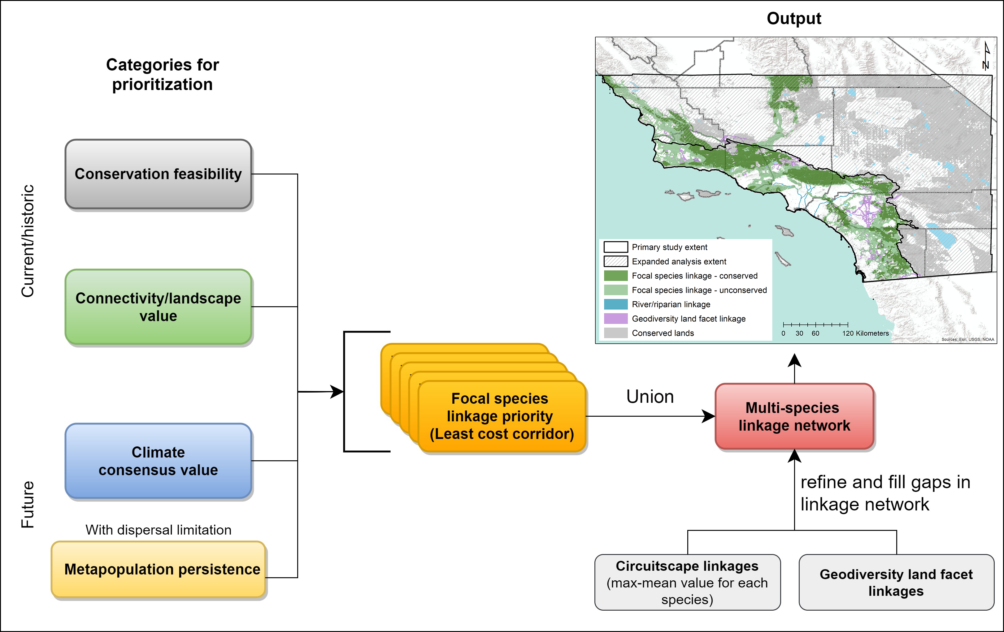
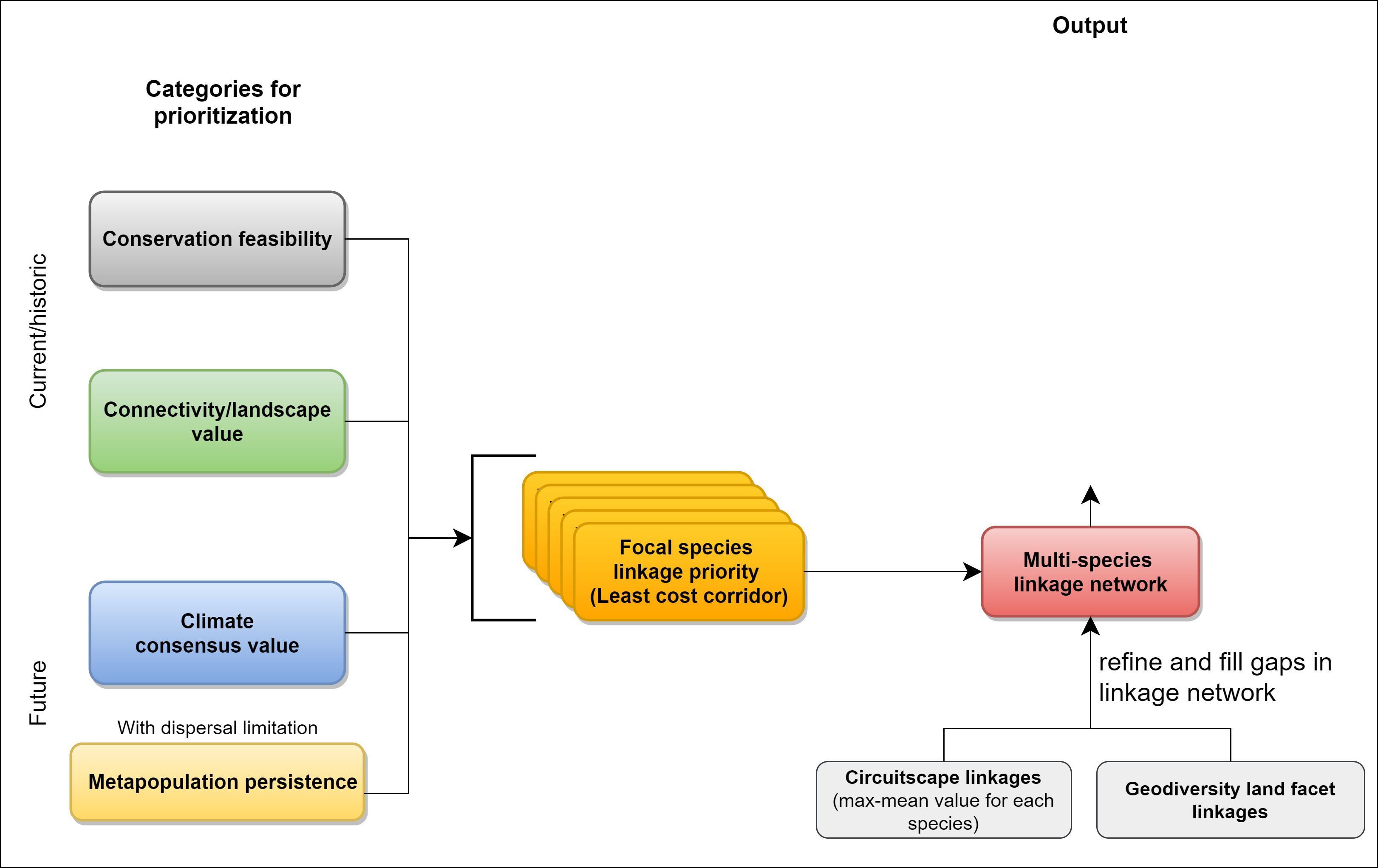
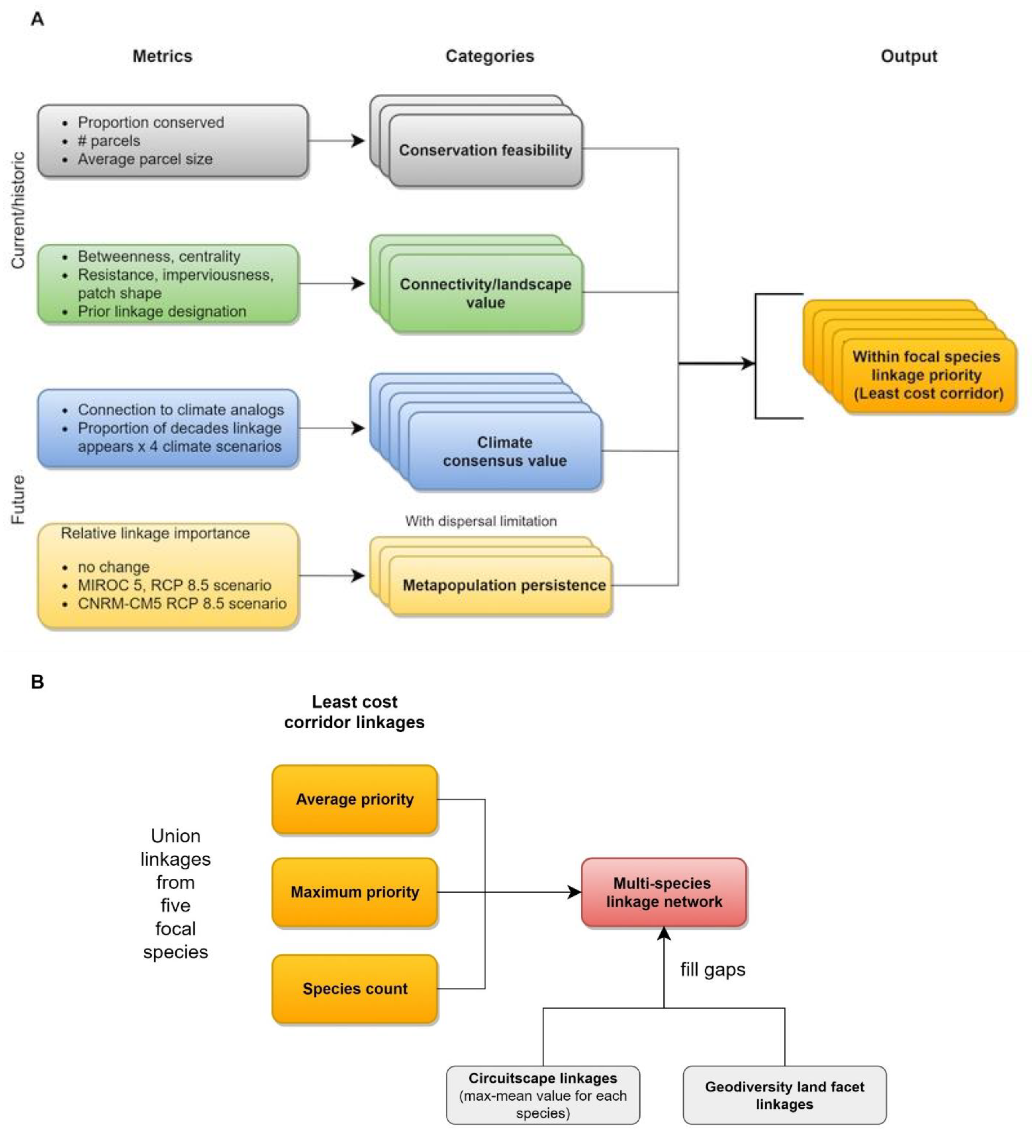
2.3. Prioritizing a Multispecies Linkage Network

Given the scale and scope of the project, prioritization was critical to achieve a realistic and implementable multispecies linkage network. To effectively prioritize linkages according to the numerous outputs produced in our modeling framework across climate scenarios and species, we developed a framework that utilized key attributes of the landscape to identify important core and linkage areas for each species, which were then included in the multispecies linkage network. To quantitatively prioritize patches within our established networks we used the Environmental Evaluation Management System (EEMS 2.02; [55]), a hierarchical decision-making toolbox in ArcGIS (ESRI, Redlands, CA, USA) based on fuzzy logic. This prioritization was a two-step process that involved first assessing the values of cores and linkage segments for each species, then ranking segments among species to be carried forward into the final network.
Prioritization with fuzzy logic requires that each metric be rescaled into fuzzy space using the EEMS tool. This involves reinterpreting metrics on a scale from being ‘completely untrue’, wherein they are assigned a value of −1, to being ‘completely true’, receiving a value of 1. For our purposes, we considered metrics on scales of low-to-high conservation value. For example, low landscape resistance would be assigned a fuzzy value of 1 (high priority value), and the highest resistances a value of −1 (low priority value) whereas linkages and cores with the highest proportion of area conserved would receive fuzzy values of 1, and low proportions would receive fuzzy values of −1.

2.3.1. Within-Species Prioritization

Our first step in prioritization was based on four main categories (Figure 3A): conservation feasibility, connectivity/landscape value, climate consensus value, and metapopulation persistence, which incorporated species-specific dispersal limitations. We assessed priority with these categories by hierarchically combining closely related metrics. Our first two prioritization categories addressed the value of linkages based on current conditions whereas the second two considered future conditions. Further details on the prioritization approach and metrics described below can be found in Section 2.1 of the Supplementary Materials S2, Figure S1, Tables S4 and S5, which describe each metric, how each value was “fuzzified”, and how metrics were combined to create the final priority linkage for each species.
Conservation feasibility combined metrics to account for factors that would facilitate or present challenges for conserving linkages within the network, including the number of parcels per unit area (unpublished data, California Department of Fish and Wildlife), average parcel size, and percent of area already conserved [56]. The parcel metrics were included to serve as a proxy for the cost of conserving a given area based on the assumption that a larger number of small parcels would likely cost more than fewer large parcels.
Connectivity and landscape value, which was based on historic conditions (in the year 2000), encompassed measures of betweenness (i.e., the number of patches that use the node as a hub) and centrality, (i.e., the number of bordering patches) calculated in the igraph package [57], habitat quality metrics including the ratio of patch edge to overall area, impervious surface cover to delineate urban areas (National Land Cover Database 2011; [33]), resistance, and whether a linkage overlapped with areas previously identified as important under the South Coast Missing Linkages (SCML; [58]) or California Essential Habitats Connectivity (CEHC; [59]) projects.
The next prioritization category considered the potential future value of each linkage under climate change. We used Climate consensus value to identify where there was a greater weight of evidence and thus, higher confidence, that a linkage would be important in the future. We calculated consensus in two ways: (1) based on connectivity to climate analogs (i.e., similarity in a location’s climate relative to another location in the future), and (2) accounting for the number of time steps in our decadal modeling a linkage persisted within each of the four climate scenarios. Our assessment of climate analogs evaluated climatic water deficit [60] which accounts for temperature and precipitation under two climate scenarios (MIROC5 and CNRM-CM5 under the RCP 8.5 emissions scenario). We assessed linkage connections based on the climatic envelopes of historic and future conditions using the Linkage Priority Mapper tool [61]. The importance of each linkage for connecting climate analogs was calculated as the climate envelope difference between current and future conditions. The climatic difference was combined with closeness, permeability, and core area values and normalized on a scale of 0 to 1 where closeness was defined as the normalized distance between the two cores a given linkage connects, permeability was the inverse of resistance, and core area value was parameterized using the climate signature of the climatic water deficit layer. To account for the value of linkages over our decadal time steps and across scenarios, we evaluated consensus assuming the greater number of times a linkage was present, the more likely it is important for connecting present and future habitat patches. Thus, linkages could be present between one to ten time periods under each of the four future scenarios for each of the five focal species.
Finally, Metapopulation persistence was based on a prioritization determined through the Linkage Priority Mapper [61] using the relative importance value described above. As with the climate analog prioritization, we calculated the metapopulation persistence value for each linkage by combining the relative importance value with closeness, permeability, and core area values where core area value was based on the habitat suitability value. We assigned the relative importance twice the weight of the other factors considered. This priority value was calculated under no change, as well as under two future scenarios (MIROC5 and CNRM-CM5 under RCP 8.5).

2.3.2. Multispecies Prioritization

Once linkages were prioritized for each species, those with highest values were selected for inclusion in the multispecies network. To assemble this network, we created a union of the cores and linkages for all species from the historic framework and developed another EEMS model to then select the portions of the union that should move forward into the final network. This model first employed a union function to combine the maximum priority value of a segment for any given species with the average value across all five species (Figure 3B). We also created a count variable to identify linkage segments that served multiple species. This addition allowed us to include important linkages through more urban areas that are constrained but may play an important role in connecting isolated urban habitat patches. We assembled the multispecies network from a union of all species’ cores and linkages using an ‘or’ function to calculate a final multispecies priority value based on segments that either had a high combined maximum and average value or served three or more species. Once we calculated the final multispecies priority value, we examined the output and determined that a threshold of 0.35 (on the fuzzy scale of −1 to 1) would allow us to delineate complete linkages while still being restrictive enough to be feasibly implemented.
We selected all segments from the multispecies union that were above this threshold to form the basis of the multispecies network. Once we established this basis using the highest priority segments from the least cost corridor models, we reviewed the output from our individual species Circuitscape models under historic conditions to account for potential differences in linkage delineation resulting from different methodological approaches. After normalizing the outputs for all species, we calculated average and maximum multispecies flow, selecting the top 20% of average flow and top 30% of maximum flow. We combined these flow surfaces and found there were gaps in our multispecies union, and so expanded linkages in these areas accordingly. We then reviewed our species-agnostic geodiversity land facet linkages and found that the facets providing connectivity along cool lower slopes, upper slopes, and peaks and ridges were well-represented by our focal species linkages. However, given the absence of a grassland-associate from our suite of focal species, only a portion of the valley and narrow valley linkages were covered by our focal species linkages. As such, we added these complementary linkage segments to the regional network. Finally, to reinforce connections through more intensely developed areas within the urban matrix, we examined and compared the geography of existing urban conservation planning efforts in the region that are focused on remnant corridors, primarily along rivers or through riparian areas (e.g., Emerald Necklace Vision Plan, Santa Ana River Parkway). We incorporated these areas into our final linkage network, labeling them as river or riparian linkages to distinguish them from linkages identified by our modeling efforts.

3. Results

3.1. Habitat Suitability, Linkage, and Metapopulation Modeling

Based on our assessments of performance using cross-validation, the models for all five focal species performed relatively well at predicting suitability of occupied habitat. The bootstrapped accuracy averaged across models and ten subsamples of data was 0.95 for owls, 0.80 for wrentit, 0.85 for woodrat, 0.83 for western toad, and 0.80 for bobcat, all based on a scale of 0 to 1.
After we generated historic least cost corridor surfaces for each species, we truncated results on a species-specific basis to establish linkages that were wide enough to accommodate movement but restricted to an area that could feasibly be conserved. Across the region, the combined core and restricted linkage network under historic conditions resulted in identification of: 22,230 km2 for big-eared woodrat, 16,840 km2 for bobcat, 14,483 km2 for California spotted owl, 11,544 km2 for western toad, and 16,568 km2 for wrentit. The union of each of these segments comprised 41,738 km2 across the region.
Under all climate scenarios for wrentit and big-eared woodrat, we found that dispersal-limitation for both species restricted the number and length of corridors that were important to the metapopulation. Furthermore, we observed that considerable habitat consolidation in the north limited the benefit of connectivity. Connectivity appeared to be most important in the future where habitat fragmentation was projected in the southern portion of our study area. For bobcat and western toad, we found that fragmentation for both species in the future reduced the overall risk to the population under any scenario because patches became separated and as such, were less likely to simultaneously experience events that would affect subpopulations (e.g., patch-scale fires). For these two species, corridors connecting patches of habitat that were projected to fragment under climate change were particularly beneficial. As a long-distance disperser, bobcats relied on long corridors, and overall, benefitted more from connectivity than the other focal species. The results for spotted owls demonstrated the most substantial climate change impacts. With most of their habitat at high elevations, spotted owls were projected to lose a substantial amount of habitat under all scenarios; therefore, there was not enough habitat remaining to support sustainable populations to the end of the century. Summary maps of the population modeling results for each species under each scenario are available in Supplementary Materials S3, Figures S2–S6.

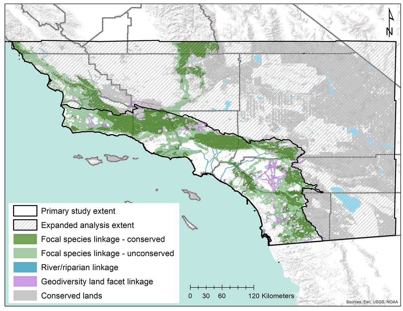
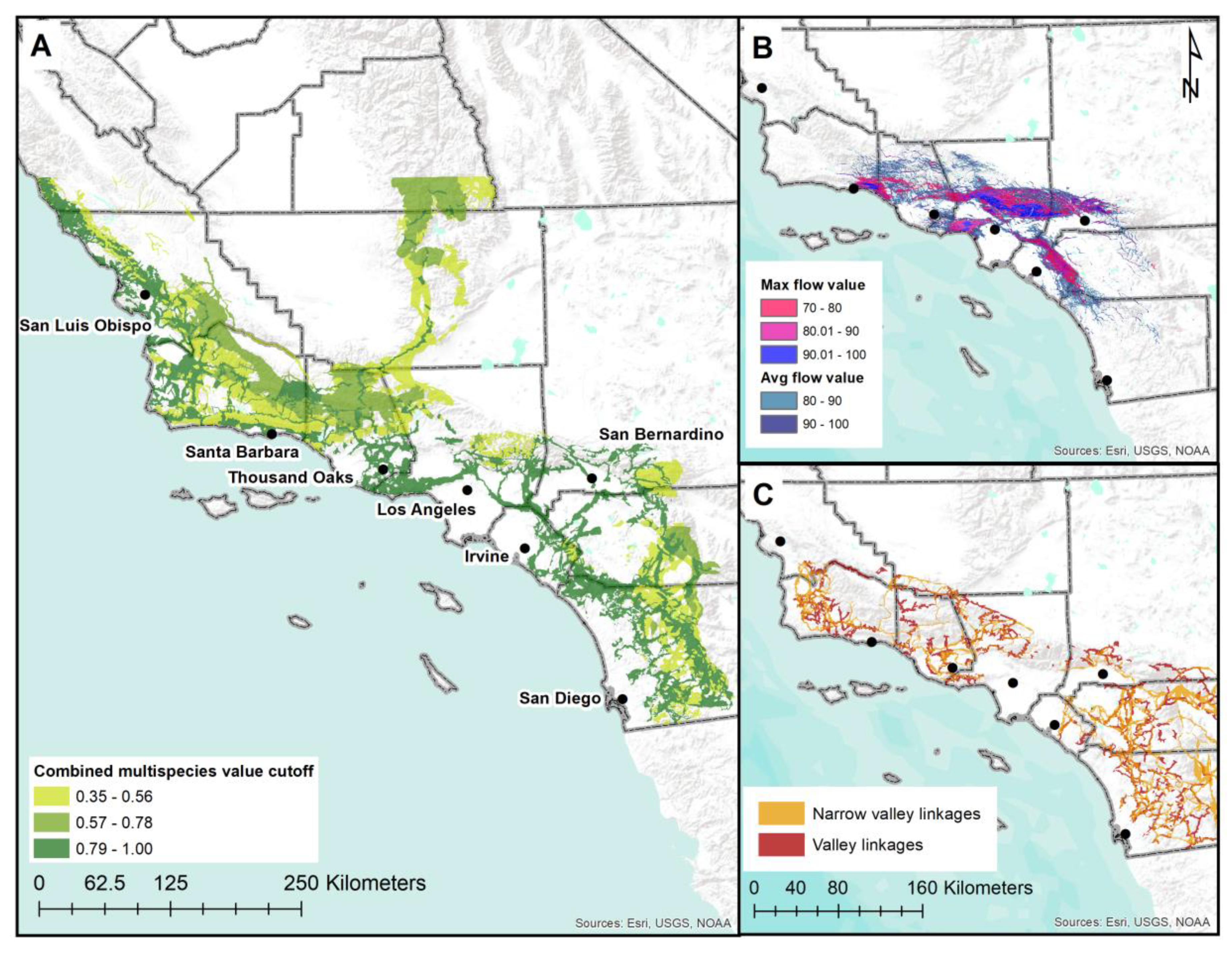
3.2. Prioritizing a Multispecies Linkage Network

After applying the threshold cutoff to the prioritized multispecies union (Figure 4A) and adding in components of the Circuitscape (Figure 4B) and geodiversity land facet linkages (Figure 4C), the final linkage network totaled 30,052 km2. The combination of Circuitscape outputs from the top 30% of the maximum flow value and top 20% of the average flow value resulted in identification 4672 km2 of linkage area. Of this total area, we added 1382 km2 to the final network after removing portions of that overlapped with the least cost corridor network and segments that identified flow through areas with very high levels of impervious surface. From the geodiversity land facet linkages, we evaluated an additional 6661 km2 of linkages in valleys and 6900 km2 in narrow valleys, 1847 km2 of which contributed to our final network after accounting for overlap with our species linkages and removing areas that were highly urbanized. Finally, the addition of riparian linkages identified in prior urban connectivity planning efforts contributed another 272 km2 to the final linkage network, connecting several otherwise isolated patches or linkages to nearby conserved lands.
The final network (Figure 5) identified linkage segments and their source (species and land facet models or river/riparian linkages described in the methods above). In addition, we identified the portions of our focal species linkages that were already conserved in large blocks (>20 km2) and labeled those as ‘conserved’. Over 55% of this final multispecies linkage network is already either fully conserved [56] or protected under conservation easements [62]. After accounting for military-owned and tribal lands, which may confer some protection from development, just under 40% or 12,140 km2 of the linkage network remained on private, unconserved lands that could be considered for acquisition for linkage implementation.

4. Discussion

Connectivity is essential to climate-smart landscape conservation strategies [4] and can strengthen ecosystem resilience to additional stressors such as habitat fragmentation [6], and disturbance [7,8]. However, planning for and implementing strategies to protect and enhance landscape connectivity under climate and land-use change requires innovative approaches that address the uncertainty in potential future conditions, demographic constraints to species persistence, and the factors that affect the feasibility of conservation actions to preserve connectivity [20]. Here, we present an approach that utilizes available biological data to design a comprehensive multispecies connectivity plan that accounts for the dynamic nature of connectivity. This approach can readily be adapted to different regions, scenarios, species, and habitats to facilitate planning at different scales and advance proactive, data-informed planning and management that fosters climate resilience for native species and habitats.
Our comprehensive methodological approach is unique both in its use of species occurrence and demographic data to develop robust biological prioritizations for connectivity planning, and in the merging of this biological data with management considerations to set achievable implementation goals for climate adaptation and enhanced connectivity. By integrating multiple approaches to modeling habitat suitability and connectivity, we created an ensemble of models that were robust beyond the results of any single modeling technique, building on the strengths of a variety of methods. The focal species approach—representing a range of movement behaviors, habitat associations, and taxonomic groups—ensured we could identify linkages that would support connectivity for the most species, thereby preserving biodiversity [15,16,17]. Our stepwise combination of least cost corridor modeling, circuit-theory based flow models, as well as species-agnostic geodiversity assessment of structural connectivity is a strategy that has been demonstrated to perform well for climate adaptive connectivity [18,19]. We observed overlap and consensus among these model results, reinforcing the importance of those areas that appeared across methods. We also identified unique areas important for connectivity not captured by our primary approach, least cost corridor modeling. Using the results of our complementary connectivity modeling methods, we added nearly 4900 km2 to our linkages, representing ~17% of the total area in the final linkage network. When combined with our assessment of the biological value of these linkages and considerations for habitat quality and feasibility of implementation, we were able to further refine our evaluation and prioritization of individual linkages to assemble a multispecies network using transparent and quantitative metrics.
To facilitate decision making under the uncertainty and dynamics of climate change, we considered climate in multiple ways and employed a scenario-based approach (sensu [63]) to examine the potential for change and consensus across approaches and climate projections. The strength of our modeling approach stems from the linkage models and feasibility assessment, which were developed for historic and existing conditions in the region and then prioritized based, in part, on the potential value of each linkage under scenarios of future climate change. Our selection of climatic projections was intended to capture the range of variability and change that is likely to be observed in southern California in the future [64], and consideration for each of these scenarios was propagated through every phase of our analysis. We addressed uncertainty in future conditions by relying on consensus among our different outputs in addition to considering the value of linkages in multiple climatic contexts (i.e., time steps and climate analogs) [5].
Undoubtedly, land-use patterns and pressure are also expected to change over the time period considered in our models. Because conservation efforts have greater potential to alter projected patterns of land-use change than climate change, we excluded temporal variation in land-use from our dynamic connectivity models. While we did not include this final step in the analysis presented here, we recognize that consideration of potential land-use changes will be an essential part of translating connectivity plans into conservation action so areas at highest risk of development can be prioritized for conservation. By integrating this information at the implementation phase, decision makers can evaluate a variety of projections of land-use change modeled under differing scenarios and revisit this analysis as projections change in response to ongoing development and conservation actions.
Our approach to prioritization of landscape connectivity integrated conservation and connectivity values, while also recognizing barriers and the importance of evaluating the potential longevity of conservation investments. By identifying spatially explicit linkages that are likely to continue to support landscape connectivity under projected future change, results from our analysis can be integrated into regional conservation and management plans that are transparent [13] and address uncertainty, using quantitative metrics that directly relate to implementation considerations, ecological value, and potential role in facilitating climate adaptation [13].
The prioritization tool we used to assemble the multispecies linkage network, the EEMS modeling toolbox, can also be employed to develop a strategy or priorities for reserve design, conservation acquisitions, or even developing management strategies to protect and enhance connectivity on conserved lands [55]. The flexibility in this framework allows for decision-making to by driven by regional or organizational needs and priorities while highlighting the conservation benefits and opportunities that can arise from proactive planning for long-term conservation goals. This flexibility can also serve to connect local, jurisdictional land-use planning with regional, landscape planning, a critical synergy to ensure meaningful efforts are implemented to preserve connectivity in dynamic landscapes.

5. Conclusions

We demonstrated a framework to assess functional connectivity under shifting conditions and evaluate and prioritize linkages that provide adaptive capacity for wildlife populations threatened by climate and land-use change. Although translating the connectivity assessment we developed into action will require coordination and communication with stakeholders working in land management and land-use and development planning [13], the strong scientific foundation we present can serve as the necessary foundation to support strategic, climate-wise planning. Our approach can be directly and widely applied to connectivity planning and implementation, particularly when considering connectivity as a key component of reserve design. In addition, the linkage network we developed can be used as an input for further prioritization, guided and designed by end-users. Specifically, prioritization of implementation actions should include future projections of land-use to ensure implementation efforts account for the threat of land-use change. By linking quantitative metrics to our corridors and prioritizing areas for conservation based on that information, our approach is transparent, and as such, can support conservation decision-making, despite the uncertainties of the cascading ecological impacts of climate change.

Supplementary Materials

The following are available online at https://www.mdpi.com/2073-445X/9/10/341/s1, S1: Detailed methods for ensemble distribution models, linkage modeling, and metapopulation models, S2: Prioritization for multispecies linkage assembly, S3: Maps of metapopulation modeling results for each scenario by species.

Author Contributions

Conceptualization, M.K.J., E.H., R.L.L., and E.C.; methodology, M.K.J., E.H., D.F., and E.C.; formal analysis, M.K.J., E.H., D.F., and E.C.; data curation, M.K.J. and D.F.; writing—original draft preparation, M.K.J.; writing—review and editing, E.H., D.F., R.L.L., and E.C.; project administration, M.K.J.; funding acquisition, M.K.J., R.L.L., and E.C. All authors have read and agreed to the published version of the manuscript.

Funding

This research was funded by the California Wildlife Conservation Board grant number WC-1541SM, Project ID#2015095 and a California State Wildlife Grant F16AF00551; Project # G1698064.

Acknowledgments

We thank partners and stakeholders at the California Department of Fish and Wildlife, particularly Hans Sin, Gail Sevrens, Terri Stewart, Ed Pert, Karen Miner, Ken Devore, and Amanda McGarry. We received support on climate model selection from Dan Cayan and Julie Kalansky at the Scripps Institution of Oceanography and are grateful for downscaled climate data provided by Alan and Lorraine Flint from the United States Geological Survey (USGS). We acknowledge the contributions of species experts and researchers who provided data and time to review species’ model inputs and outputs for us: Seth Riley (National Park Service); Lisa Lyren (Naval Facilities and Engineering Command); Scott Tremor (San Diego Natural History Museum); Kurt Anderson (University of California, Riverside); Stephen Rice (formerly San Diego State University); Robert Fisher and Carlton Rochester (USGS); Kris Preston (San Diego Management and Monitoring Program and USGS); Phil Unitt (San Diego Natural History Museum). We are also appreciative of data sharing for western toad by members of HerpMapper and NA HERP. Expertise and support were provided for use of prioritization programs and Data Basin by Conservation Biology staff members John Gallo, Tim Sheehan, and Kai Henifin. Amber Pairis from the Climate Science Alliance provided project support, encouragement, and supported project promotion and communication. Michelle Kinzel (SDSU) provided data analysis support during the project.

Conflicts of Interest

The authors declare no conflict of interest.

References

  1. IPCC. Synthesis Report. Contribution of Working Groups I, II and III to the Fifth Assessment Report of the Intergovernmental Panel on Climate Change; Core Writing Team, Pachauri, R.K., Meyer, L.A., Eds.; IPCC: Geneva, Switzerland, 2014; p. 151. [Google Scholar]
  2. Parmesan, C. Ecological and evolutionary responses to recent climate change. Annu. Rev. Ecol. Evol. Syst. 2006, 37, 637–669. [Google Scholar] [CrossRef] [Green Version]
  3. McRae, B.H.; Hall, S.A.; Beier, P.; Theobald, D.M. Where to Restore Ecological Connectivity? Detecting Barriers and Quantifying Restoration Benefits. PLoS ONE 2012, 7, e52604. [Google Scholar] [CrossRef] [PubMed]
  4. Heller, N.E.; Zavaleta, E.S. Biodiversity management in the face of climate change: A review of 22 years of recommendations. Biol. Conserv. 2009, 142, 14–32. [Google Scholar] [CrossRef]
  5. Keeley, A.T.H.; Ackerly, D.D.; Cameron, D.R.; Heller, N.E.; Huber, P.R.; Schloss, C.A.; Thorne, J.H.; Merenlender, A.M. New concepts, models, and assessments of climate-wise connectivity. Environ. Res. Lett. 2018, 13, 073002. [Google Scholar] [CrossRef]
  6. Beier, P.; Gregory, A.J. Desperately seeking sTable 50-year-old landscapes with patches and long, wide corridors. PLoS Biol. 2012, 10, e1001253. [Google Scholar] [CrossRef] [Green Version]
  7. Noss, R.F. Landscape connectivity: Different functions at different scales. In Landscape linkages and Biodiversity; Hudson, W.E., Ed.; Island Press: Washington, DC, USA, 1991; pp. 27–39. [Google Scholar]
  8. Hilty, J.A.; Lidicker, W., Jr.; Merenlender, A.M. Corridor Ecology: The Science and Practice of Linking Landscapes for Biodiversity Conservation; Island Press: Washington, DC, USA, 2006; ISBN 1559630477. [Google Scholar]
  9. Brown, J.H.; Kodric-Brown, A. Turnover Rates in Insular Biogeography: Effect of Immigration on Extinction. Ecology 1977, 58, 445–449. [Google Scholar] [CrossRef] [Green Version]
  10. Simberloff, D.; Farr, J.A.; Cox, J.; Mehlman, D.W. Movement corridors: Conservation bargains or poor investments? Conserv. Biol. 1992, 6, 493–504. [Google Scholar] [CrossRef]
  11. Hannah, L.; Midgley, G.F.; Millar, D. Climate change-integrated conservation strategies. Glob. Ecol. Biogeogr. 2002, 11, 485–495. [Google Scholar] [CrossRef] [Green Version]
  12. Saura, S.; Bertzky, B.; Bastin, L.; Battistella, L.; Mandrici, A.; Dubois, G. Protected area connectivity: Shortfalls in global targets and country-level priorities. Biol. Conserv. 2018, 219, 53–67. [Google Scholar] [CrossRef]
  13. Keeley, A.T.H.; Beier, P.; Creech, T.; Jones, K.; Jongman, R.H.G.; Stonecipher, G.; Tabor, G.M. Thirty years of connectivity conservation planning: An assessment of factors influencing plan implementation. Environ. Res. Lett. 2019, 14, 103001. [Google Scholar] [CrossRef]
  14. Luque, S.; Saura, S.; Fortin, M.-J. Landscape connectivity analysis for conservation: Insights from combining new methods with ecological and genetic data. Landsc. Ecol. 2012, 27, 153–157. [Google Scholar] [CrossRef]
  15. Dilkina, B.; Houtman, R.; Gomes, C.P.; Montgomery, C.A.; McKelvey, K.S.; Kendall, K.; Graves, T.A.; Bernstein, R.; Schwartz, M.K. Trade-offs and efficiencies in optimal budget-constrained multispecies corridor networks. Conserv. Biol. 2017, 31, 192–202. [Google Scholar] [CrossRef]
  16. Gippoliti, S.; Battisti, C. More cool than tool: Equivoques, conceptual traps and weaknesses of ecological networks in environmental planning and conservation. Land Use policy 2017, 68, 686–691. [Google Scholar] [CrossRef]
  17. Albert, C.H.; Rayfield, B.; Dumitru, M.; Gonzalez, A. Applying network theory to prioritize multispecies habitat networks that are robust to climate and land-use change. Conserv. Biol. 2017, 31, 1383–1396. [Google Scholar] [CrossRef] [PubMed] [Green Version]
  18. Brost, B.M.; Beier, P. Comparing linkage designs based on land facets to linkage designs based on focal species. PLoS ONE 2012, 7, e48965. [Google Scholar] [CrossRef] [Green Version]
  19. Krosby, M.; Breckheimer, I.; Pierce, D.J.; Singleton, P.H.; Hall, S.A.; Halupka, K.C.; Gaines, W.L.; Long, R.A.; McRae, B.H.; Cosentino, B.L.; et al. Focal species and landscape “naturalness” corridor models offer complementary approaches for connectivity conservation planning. Landsc. Ecol. 2015, 30, 2121–2132. [Google Scholar] [CrossRef]
  20. McGuire, J.L.; Lawler, J.J.; McRae, B.H.; Nuñez, T.A.; Theobald, D.M. Achieving climate connectivity in a fragmented landscape. Proc. Natl. Acad. Sci. USA 2016, 113, 7195–7200. [Google Scholar] [CrossRef] [Green Version]
  21. Hanski, I. Metapopulation Ecology; Oxford University Press: Oxford, UK, 1999; p. 313. ISBN 0198540655. [Google Scholar]
  22. Bengtsson, J.; Angelstam, P.; Elmqvist, T.; Emanuelsson, U.; Folke, C.; Ihse, M.; Moberg, F.; Nyström, M. Reserves, Resilience and Dynamic Landscapes. AMBIO 2003, 32, 389–396. [Google Scholar] [CrossRef]
  23. Vos, C.C.; van der Hoek, D.C.J.; Vonk, M. Spatial planning of a climate adaptation zone for wetland ecosystems. Landsc. Ecol. 2010, 25, 1465–1477. [Google Scholar] [CrossRef]
  24. Nuñez, T.A.; Lawler, J.J.; McRae, B.H.; Pierce, D.J.; Krosby, M.B.; Kavanagh, D.M.; Singleton, P.H.; Tewksbury, J.J. Connectivity Planning to Address Climate Change. Conserv. Biol. 2013, 27, 407–416. [Google Scholar] [CrossRef]
  25. Penrod, K.; Beier, P.; Garding, E.; Cabañero, C. A Linkage Network for the California Deserts; Technical Report for the Bureau of Land Management and The Wildlands Conservancy: Fair Oaks, CA, USA, February 2012.
  26. Underwood, E.C.; Viers, J.H.; Klausmeyer, K.R.; Cox, R.L.; Shaw, M.R. Threats and biodiversity in the mediterranean biome. Divers. Distrib. 2009, 15, 188–197. [Google Scholar] [CrossRef]
  27. Syphard, A.D.; Radeloff, V.C.; Keeley, J.E.; Hawbaker, T.J.; Clayton, M.K.; Stewart, S.I.; Hammer, R.B. Human influence on California fire regimes. Ecol. Appl. 2007, 17, 1388–1402. [Google Scholar] [CrossRef]
  28. Franklin, J.; Wejnert, K.E.; Hathaway, S.A.; Rochester, C.J.; Fisher, R.N. Effect of species rarity on the accuracy of species distribution models for reptiles and amphibians in southern California. Divers. Distrib. 2009, 15, 167–177. [Google Scholar] [CrossRef]
  29. Daly, C. Guidelines for assessing the suitability of spatial climate data sets. Int. J. Climatol. 2006, 26, 707–721. [Google Scholar] [CrossRef]
  30. U.S. Geological Survey National Elevation Dataset. Sioux Falls, SD: EROS. 2009. Available online: http://viewer.nationalmap.gov/viewer/ (accessed on 15 July 2016).
  31. Flint, L.E.; Flint, A.L. Downscaling future climate scenarios to fine scales for hydrologic and ecological modeling and analysis. Ecol. Process. 2012, 1, 2. [Google Scholar] [CrossRef] [Green Version]
  32. Pierce, D.W.; Cayan, D.R.; Thrasher, B.L. Statistical Downscaling Using Localized Constructed Analogs (LOCA)*. J. Hydrometeorol. 2014, 15, 2558–2585. [Google Scholar] [CrossRef]
  33. Jin, S.; Yang, L.; Danielson, P.; Homer, C.; Fry, J.; Xian, G. A comprehensive change detection method for updating the National Land Cover Database to circa 2011. Remote Sens. Environ. 2013, 132, 159–175. [Google Scholar] [CrossRef] [Green Version]
  34. Zimmerman, J.K.H.; Carlisle, D.M.; May, J.T.; Klausmeyer, K.R.; Grantham, T.E.; Brown, L.R.; Howard, J.K. Patterns and magnitude of flow alteration in California, USA. Freshw. Biol. 2018, 63, 859–873. [Google Scholar] [CrossRef] [Green Version]
  35. Jenness, J. DEM Surface Tools. Available online: http://www.jennessent.com/arcgis/surface_area.htm (accessed on 15 July 2016).
  36. R Core Team. R: A Language and Environment for Statistical Computing; R Core Team: Vienna, Austria, 2017. [Google Scholar]
  37. Wood, S.N. Fast stable restricted maximum likelihood and marginal likelihood estimation of semiparametric generalized linear models. J. R. Stat. Soc. Ser. B 2011, 73, 3–36. [Google Scholar] [CrossRef] [Green Version]
  38. biomod2: Ensemble Platform for Species Distribution Modeling. Available online: https://cran.r-project.org/web/packages/biomod2/index.html (accessed on 1 August 2020).
  39. Hijmans, R.J.; Phillips, S.; Leathwick, J.; Elith, J. Package ‘dismo’’-Species Distribution Modeling’. Circles 2017, 9, 1–68. [Google Scholar]
  40. Shirk, A.; McRae, B.H. Gnarly Landscape Utilities: Core Mapper User Guide; The Nature Conservancy: Fort Collins, CO, USA, 2013. [Google Scholar]
  41. Adriaensen, F.; Chardon, J.P.; De Blust, G.; Swinnen, E.; Villalba, S.; Gulinck, H.; Matthysen, E. The application of ‘least-cost’ modelling as a functional landscape model. Landsc. Urban Plan. 2003, 64, 233–247. [Google Scholar] [CrossRef]
  42. Keeley, A.T.H.; Beier, P.; Gagnon, J.W. Estimating landscape resistance from habitat suitability: Effects of data source and nonlinearities. Landsc. Ecol. 2016, 31, 2151–2162. [Google Scholar] [CrossRef]
  43. Trainor, A.M.; Walters, J.R.; Morris, W.F.; Sexton, J.; Moody, A. Empirical estimation of dispersal resistance surfaces: A case study with red-cockaded woodpeckers. Landsc. Ecol. 2013, 28, 755–767. [Google Scholar] [CrossRef]
  44. Mateo-Sánchez, M.C.; Balkenhol, N.; Cushman, S.; Pérez, T.; Domínguez, A.; Saura, S. A comparative framework to infer landscape effects on population genetic structure: Are habitat suitability models effective in explaining gene flow? Landsc. Ecol. 2015, 30, 1405–1420. [Google Scholar] [CrossRef]
  45. McRae, B.H.; Kavanagh, D.M. Linkage Mapper Connectivity Analysis Software; The Nature Conservancy: Seattle, WA, USA, 2011. [Google Scholar]
  46. McRae, B.H.; Dickson, B.G.; Keitt, T.H.; Shah, V.B. Using Circuit Theory to Model Connectivity in Ecology, Evolution, and Conservation. Ecology 2008, 89, 2712–2724. [Google Scholar] [CrossRef] [PubMed]
  47. Bezanson, J.; Edelman, A.; Karpinski, S.; Shah, V.B. Julia: A fresh approach to numerical computing. SIAM Rev. 2017, 59. [Google Scholar] [CrossRef] [Green Version]
  48. Anantharaman, R.; Hall, K.; Shah, V.; Edelman, A. Circuitscape in Julia: High performance connectivity modelling to support conservation decisions. arXiv 2019, arXiv:1906.03542. [Google Scholar]
  49. Comer, P.J.; Pressey, R.L.; Hunter, M.L.; Schloss, C.A.; Buttrick, S.C.; Heller, N.E.; Tirpak, J.M.; Faith, D.P.; Cross, M.S.; Shaffer, M.L. Incorporating geodiversity into conservation decisions. Conserv. Biol. 2015, 29, 692–701. [Google Scholar] [CrossRef]
  50. Theobald, D.M.; Harrison-Atlas, D.; Monahan, W.B.; Albano, C.M. Ecologically-relevant maps of landforms and physiographic diversity for climate adaptation planning. PLoS ONE 2015, 10, e0143619. [Google Scholar] [CrossRef] [Green Version]
  51. Beier, P.; Brost, B. Use of land facets to plan for climate change: Conserving the arenas, not the actors. Conserv. Biol. 2010, 24, 701–710. [Google Scholar] [CrossRef]
  52. Brost, B.M.; Beier, P. Use of land facets to design linkages for climate change. Ecol. Appl. 2012, 22, 87–103. [Google Scholar] [CrossRef]
  53. Jenness, J.; Brost, B.; Beier, P. Land Facet Corridor Designer: Extension for ArcGIS; Jenness Enterprises: Flagstaff, AZ, USA, 2013; p. 110. [Google Scholar]
  54. Akçakaya, H.R.; Root, W.T. Linking Landscape Data with Population Viability Analysis (Version 5.0); Applied Mathematics: Setaukey, NY, USA, 2005. [Google Scholar]
  55. Sheehan, T.; Gough, M. A platform-independent fuzzy logic modeling framework for environmental decision support. Ecol. Inform. 2016, 34, 92–101. [Google Scholar] [CrossRef]
  56. GreenInfo Network California Protected Areas Database. 2018. Available online: https://www.calands.org/cpad/ (accessed on 31 October 2018).
  57. Csardi, G.; Nepusz, T. The igraph software package for complex network research. Inter J. Complex Syst. 2006, 1695, 1–9. [Google Scholar]
  58. South Coast Wildlands. South Coast Wildlands South Coast Missing Linkages: A Wildland Network for the South Coast Ecoregion; South Coast Wildlands: Fair Oaks, CA, USA, 2008; 67p. [Google Scholar]
  59. Spencer, W.D.; Beier, P.; Penrod, K.; Paulman, K.; Rustigian-Romsos, H.; Strittholt, J.; Parisi, M.; Pettler, A. California Essential Habitat Connectivity Project: A Strategy for Conservation a Connected California; Prepared for California Department of Transportation, California Department of Fish and Game, and Federal Highways Administration: Sacramento, CA, USA, 2010; p. 313.
  60. Flint, L.E.; Flint, A.L.; Thorne, J.H.; Boynton, R. Fine-scale hydrologic modeling for regional landscape applications: The California Basin Characterization Model development and performance. Ecol. Process. 2013, 2, 25. [Google Scholar] [CrossRef] [Green Version]
  61. Gallo, J.A.; Greene, R. Connectivity Analysis Software for Estimating Linkage Priority; Conservation Biology Institute: Corvallis, OR, USA, 2018. [Google Scholar]
  62. GreenInfo Network California Conservation Easements Database. 2018. Available online: https://www.calands.org/cced/ (accessed on 31 October 2018).
  63. Peterson, G.D.; Cumming, G.S.; Carpenter, S.R. Scenario planning: A tool for conservation in an uncertain world. Conserv. Biol. 2003, 17, 358–366. [Google Scholar] [CrossRef] [Green Version]
  64. Lynn; Elissa; Schwarz, A.; Anderson, J.; Correa, M. Perspectives and Guidance for Climate Change Analysis; Technical Report for California Department of Water Resources (DWR) and Climate Change Technical Advisory Group (CCTAG): Sacramento, CA, USA, August 2015.
Figure 1. Map depicting the primary study area within southern California, U.S.A., with conserved lands identified in green and urban development in gray. The hatched area represents the expanded analytical extent.
Land 09 00341 g001
Figure 2. Diagram of the analytical process for patch, linkage, and metapopulation modeling. Analysis starts with occurrence points for focal species and their association with climatic and environmental variables. From those points, suitability maps are generated under historic and future conditions. Suitability is converted to resistance, which is used in linkage modeling. Both the habitat suitability and the linkages inform dynamic population models which are then used in linkage prioritization (see Figure 3).
Land 09 00341 g002
Figure 3. Conceptual model of how individual focal species linkages are assembled into a single multispecies network. (A) Depicts the within-species prioritization of least cost corridor linkages for each focal species. Prioritization was based on metrics that were grouped into four categories, conservation feasibility, connectivity and landscape value, climate consensus, and metapopulation persistence. (B) Illustrates how the multispecies linkage network was assembled from the union of the within-species prioritization values with linkages from the Circuitscape and land facet analyses used to fill gaps in the network.
Land 09 00341 g003
Figure 4. Maps depicting the outputs of the three linkage modeling approaches used to assemble the final linkage network. (A) Shows the selected threshold for the prioritized least cost corridor models; (B) Depicts Circuitscape outputs reflecting the combined top 20% of the average normalized percent flow and top 30% of the maximum percent flow for all species; (C) Identifies the selected geodiversity land facet linkages through valleys and narrow valleys.
Land 09 00341 g004
Figure 5. Final multispecies linkage map with different linkage types identified by the source for each type. Focal species linkages were derived from species-based modeling. Map depicts the full linkage network including large blocks of conserved lands important for climate connectivity and linkage segments yet to be conserved. River/riparian linkages follow major drainages to provide urban linkages. Finally, the geodiversity land facet linkages represent valleys and narrow valleys corridors that were added to complement the species-based linkages.
Land 09 00341 g005
Table 1. Environmental and climatic variables used in species distribution models.
NameDescription and SourceTime Variant
ClimateSource: Downscaled (to 90 m) PRISM, MIROC5 RCP4.5, MIROC5 RCP8.5, CNRM CM5 RCP4.5, CNRM CM5 RCP8.5
Bioclim 1Mean temperatureYes
Bioclim 2Mean diurnal range (mean of monthly (max temperature-minimum temperature))Yes
Bioclim 4Temperature Seasonality (Monthly standard deviation *100)Yes
Bioclim 6Minimum temperature of the coldest monthYes
Bioclim 12Mean precipitationYes
Bioclim 14Precipitation of the driest monthYes
Bioclim 15Precipitation seasonality (coefficient of variation across months)Yes
Land- useSource: National Land Cover Database 2011 [33]
Impervious surfacesUsed as a proxy for urban land coverNo
Water ResourcesSource: [34]
Distance to seasonal streamsEuclidean distance to streams with low probability of year-round flowNo
Distance to perennial streamsEuclidean distance to streams with high probability of year-round flowNo
Stream densityDensity of all streams within a 5-km moving windowNo
TopographySource: National Elevation Dataset [30]
Roughness IndexTotal curvature calculated with DEM Surface Tools [35]No
Percent SlopeDerived from National Elevation DatasetNo

