Operationalizing Vulnerability: Land System Dynamics in a Transfrontier Conservation Area
by
Andrea Elizabeth Gaughan
1,*, 
Forrest Robert Stevens
1,
Narcisa Gabriela Pricope
2,
Joel Hartter
3,
Lin Cassidy
4 and
Jonathan Salerno
5 1
Department of Geography and Geosciences, University of Louisville, 213 Lutz Hall, Louisville, KY 40292, USA
2
Department of Earth and Ocean Sciences, University of North Carolina Wilmington, 601 S College Rd., Wilmington, NC 28403, USA
3
Environmental Studies Program, University of Colorado Boulder, 4001 Discovery Dr., Boulder, CO 80303, USA
4
Independent Research Consultant, P.O. Box 233, Maun, Ngamiland District 00000, Botswana
5
Department of Human Dimensions of Natural Resources, Colorado State University, 1480 Campus Delivery, Fort Collins, CO 80523-1480, USA
*
Author to whom correspondence should be addressed.
Land 2019, 8(7), 111; https://doi.org/10.3390/land8070111
Submission received: 16 May 2019
/
Revised: 9 July 2019
/
Accepted: 11 July 2019
/
Published: 16 July 2019
Abstract
:Understanding how individuals, communities, and populations vary in their vulnerability requires defining and identifying vulnerability with respect to a condition, and then developing robust methods to reliably measure vulnerability. In this study, we illustrate how a conceptual model translated via simulation can guide the real-world implementation of data collection and measurement of a model system. We present a generalizable statistical framework that specifies linkages among interacting social and biophysical components in complex landscapes to examine vulnerability. We use the simulated data to present a case study in which households are vulnerable to conditions of land function, which we define as the provision of goods and services from the surrounding environment. We use an example of a transboundary region of Southern Africa and apply a set of hypothesized, simulated data to illustrate how one might use the framework to assess vulnerability based on empirical data. We define vulnerability as the predisposition of being adversely affected by environmental variation and its impacts on land uses and their outcomes as exposure (E), mediated by sensitivity (S), and mitigated by adaptive capacity (AC). We argue that these are latent, or hidden, characteristics that can be measured through a set of observable indicators. Those indicators and the linkages between latent variables require model specification prior to data collection, critical for applying the type of modeling framework presented. We discuss the strength and directional pathways between land function and vulnerability components, and assess their implications for identifying potential leverage points within the system for the benefit of future policy and management decisions.
1. Introduction
The ability to detect and monitor the relationship between household vulnerability, resource use, and land system function requires a combination of conceptual understanding and optimization modeling techniques [1,2,3,4]. Environmental change impacts the vulnerability of people and communities in a myriad of well-documented ways [5,6,7]. Specification is required, in each case, for what it means to be vulnerable, and how vulnerability can be measured in order to improve our understanding of any given social–ecological system (SES). Furthermore, while intuitively vulnerability is associated with susceptibility to some phenomenon (e.g., climate change, market fluctuations, resource access, wildfire), defining and measuring vulnerability is extremely complex [8,9,10].
Theoretical traditions from political ecology, human geography and other disciplines covering hazards and climate change inform varying definitions of vulnerability [11,12,13,14,15]. Such definitions generally overlap, but attributes in their own contexts offer strengths and weaknesses for quantifying and measuring vulnerability. In addition, a social–ecological perspective provides a holistic approach in describing vulnerability, where human and environmental components of a given system are interlinked [8,14]. This perspective emphasizes social and biophysical vulnerabilities and the various adaptation mechanisms implemented by society in the face of environmental change [14,16,17]. A systems-based social–ecological framework is best placed to model the complexity of the dynamics and linkages between human and natural components of a given system [18]. Describing and quantifying these linkages can help formulate explicit policies and management actions that affect vulnerability for a specific system and across multiple scales.
In this paper, we first propose an adapted definition of vulnerability to help bridge the gaps separating disciplinary traditions and between science and practice with a specific focus on land systems. We then demonstrate how to operationalize vulnerability in an explicit model, which can guide empirical measurement and policy recommendations at different system scales. Finally, we illustrate how to apply this model to inform research design and data collection using simulated data from the Kavango–Zambezi Transfrontier Conservation Area (KAZA-TFCA) in Southern Africa. The primary goal is to introduce an approach to quantifying vulnerability through a robust theoretical framing coupled with a statistical model that provides easily communicable information towards management and policy decisions in a SES.
1.1. Theoretical Framing
Multiple research traditions have framed the definition, the scale, the conceptual framing, and the ability to measure vulnerability [5,8,9,10,15,19,20] (see [21] for an extensive review). Entitlement theory [22] and the sustainable livelihoods framework [23] provide a foundational platform from which the social dimensions of vulnerability are well articulated, while natural hazards and climate change literature represents two dominant strands of framing for the concept of vulnerability. From the natural hazards perspective, vulnerability stems from the risk of being exposed to an undesirable outcome, which may result from some type of pre-existing condition or characteristic of the population or system [12,23,24,25]. Vulnerability to climate change is defined and contextualized largely from the Intergovernmental Panel on Climate Change (IPCC) assessment reports using three components (exposure, sensitivity, and adaptive capacity) to determine the degree to which a system is susceptible to climate change and the associated social impacts and responses [26,27]. In 2014, the IPCC redefined vulnerability discrete from exposure, as “the propensity or predisposition to be adversely affected”, conceptualizing it as a “product of intersecting social processes that result in inequalities in socioeconomic status and income, as well as in exposure” [28]. This second definition addresses social marginalization explicitly, building on work such as Kasperson and Kasperson (2001) and Birkmann (2013) who view vulnerability as operating in a place-specific context, where those most vulnerable are often the most marginalized along lines of wealth, education, ethnicity, gender, age, class, and health. Different theories conceptualize vulnerability in ways that reflect their varying objectives for more directed and effective policy measures in a specific system [6,11,12,14,29]. However, Costa and Kropp (2013) point out the convergence of vulnerability definitions when applied empirically at the case study level, with various components operationalized through similar indicators. More recently, various studies modify or combine aspects of previous vulnerability frameworks or definitions along with aspects from sustainable livelihood or resilience approaches [11,30]. Including livelihood variation and agency are arguably necessary for quantifying system metrics that characterize vulnerability [27].
While we acknowledge multiple useful definitions and theories informing vulnerability, we have explicit interest in operationalizing the mechanisms that drive vulnerable outcomes for people resulting from environmental changes (e.g., soil fertility loss, drought or flooding). We define operationalization as the process by which components, such as vulnerability, of a social–ecological system is both quantified empirically and made useful for decision-making. Further, this goal requires the flexibility of a land systems (i.e., spatial composition of land units consisting of different land covers and uses) perspective [1,31] to account for various social–ecological components and their interactions, while also describing the system and its processes in order to meaningfully inform policy and interventions at multiple scales ([2,4]).
We adapt a vulnerability framework from Turner et al. (2003a, b) which identifies linkages between the social and biophysical components of a SES to reflect properties specific to exposure, sensitivity and adaptive capacity in combination with a livelihoods framework [32]. The original framework from Turner et al. enfolded into the concept of resilience other key components of vulnerability, including adaptive capacity. However, arguably, it is the human agency and decision-making underlying adaptation that we need to account for with vulnerability models. While resilience and adaptive capacity have been used interchangeably in the literature [33], resilience, an ecologically-based term, describes a system’s ability to adjust, modify, or change its characteristics in response to shocks or stress [30,31]. In contrast, adaptive capacity better captures the human agency and diversity of behaviors and responses humans make in a system [34].
With this focus in mind, we define vulnerability as the predisposition of being adversely affected by variability in some process as a function of exposure (E), mediated by sensitivity (S) and adaptive capacity (AC). In the land systems context, exposure represents the spatiotemporal nature of land uses and the environmental gradients that affect them. Sensitivity represents land use outcomes, and is influenced by the degree to which a household is exposed to the land system. This interaction is mediated by the household adaptive capacity, or resources and ability to alter or respond to change.
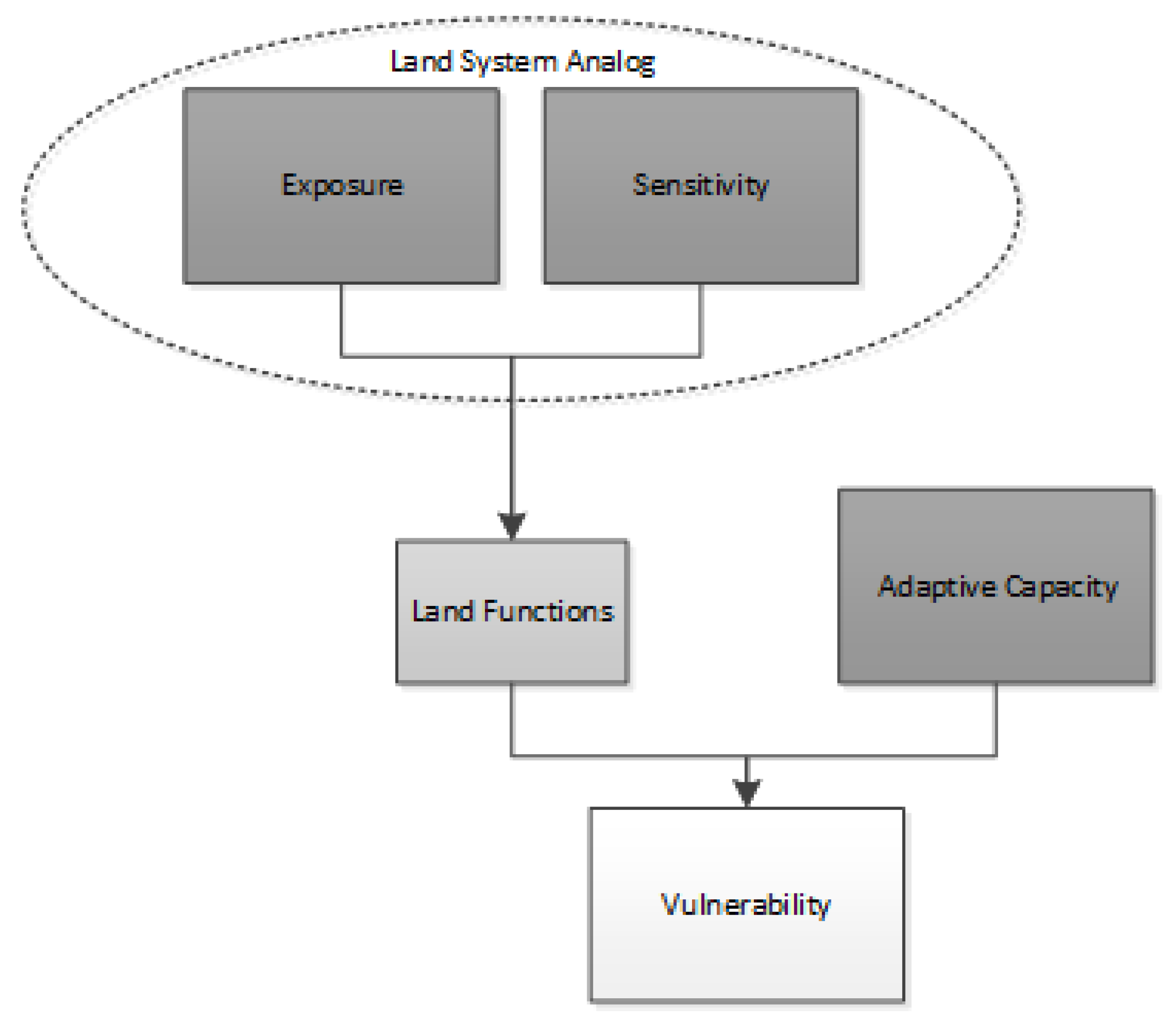
We argue that this framing to describe vulnerability is useful and can be formalized into a statistical model in order to test hypotheses by quantifying linkages of the system components. Combined, exposure and sensitivity capture land functions but changes in adaptive capacity at the household level can strongly influence, directly and indirectly, how strongly the reliance on land functions impacts variation in vulnerability (Figure 1). We acknowledge that defining vulnerability involves applying normative value judgements [10], and making assumptions regarding the level, or scale, of interest [35]. These assumptions have consequences, but assigning value to the components of vulnerability is necessary and a land systems lens is well suited to explain mechanisms driving consequential outcomes and to facilitate evidence-based decision-making in social–ecological systems [4].
1.2. A Structural Equation Model of Vulnerability
The modeling approach we propose is a structural equation model (SEM) to examine the strength and direction of relationships among the latent (not directly measurable) properties of vulnerability, exposure, sensitivity, and adaptive capacity [36]. We acknowledge that the functional forms with which to quantify or approximate household vulnerability and associated measures of exposure, sensitivity and adaptive capacity are diverse, and vary based primarily on definitions appropriate to specific contexts [8,37]. However, we address this challenge by treating vulnerability and associated components as latent constructs, which is conceptually flexible in allowing a diversity of potential definitions to be applied to these components. Being latent, vulnerability is not something that can be measured directly [10] but manifested (and defined) through measurable indicators (e.g., nutritional intake, morbidity, and mortality, food insecurity, etc.). We contend that the components that combine to create that vulnerability, namely sensitivity, exposure, and adaptive capacity, are similar to latent characteristics that can only be defined and estimated through multiple, correlated but measurable, indicators. This is described by Bollen (2002) as “local independence.” Thus, a model structure that accounts for both direct and indirect relationships, a duality of influence reflected by the indicators measured, can be used for understanding how the components of vulnerability interact in a given system [38]. Additional introduction and explanations of structural equation models are found in the following sources [39,40,41].
An SEM approach has been applied to different social–ecological contexts and at the household level [38,42,43,44] and specifically in the African context [45]. For example, a theoretical framing and application of SEM from Dang et al. (2014) gives insight into Vietnamese households’ intention to adapt to climate change based on socioeconomic factors and resource access [44]. Asah (2008) illustrates the generalizability and usefulness of an SEM combined with a strong SES framework for an agriculturalist system in the Lake Chad basin [38]. Specifying and measuring the correct, underlying indicators will be system specific, but a generalizable model form provides a platform from which key relationships between system components are interrogated for the system under study.
Despite these examples, SEM is not well represented in the land change modeling community [46]. This may be a byproduct of unfamiliarity with the statistical assumptions or difficulty in constructing concrete, but still useful sets of measures that reflects the complexity of land systems and land change. Yet, SEM provides an appealing approach for marrying theoretical relationships with measurable aspects of land systems, allowing us to theorize trade-offs in land use activities and subsequent land system processes as it links social and biophysical components of a system at multiple scales. The ability of the SEM to assess direct and indirect relationships means that one identified or hypothesized association can be modeled to interact with another causal relation. Therefore, one measured or latent component to the model might affect or be associated with changes in another component via multiple paths, which is exactly the kind of complexity captured by the proposed vulnerability model discussed here. The statistical power to decompose correlations and covariance between measured components, and trace the structure of associations through paths incorporated into the model while accounting for direct and indirect relationships, is the critical piece for quantifying how the components of vulnerability interact with one another. The next section introduces the conceptual approach along with further detail of the statistical structure we propose for quantifying household-level vulnerability in a land systems context.
2. Conceptual Approach and Methods
2.1. A Structural Model for Household Vulnerability
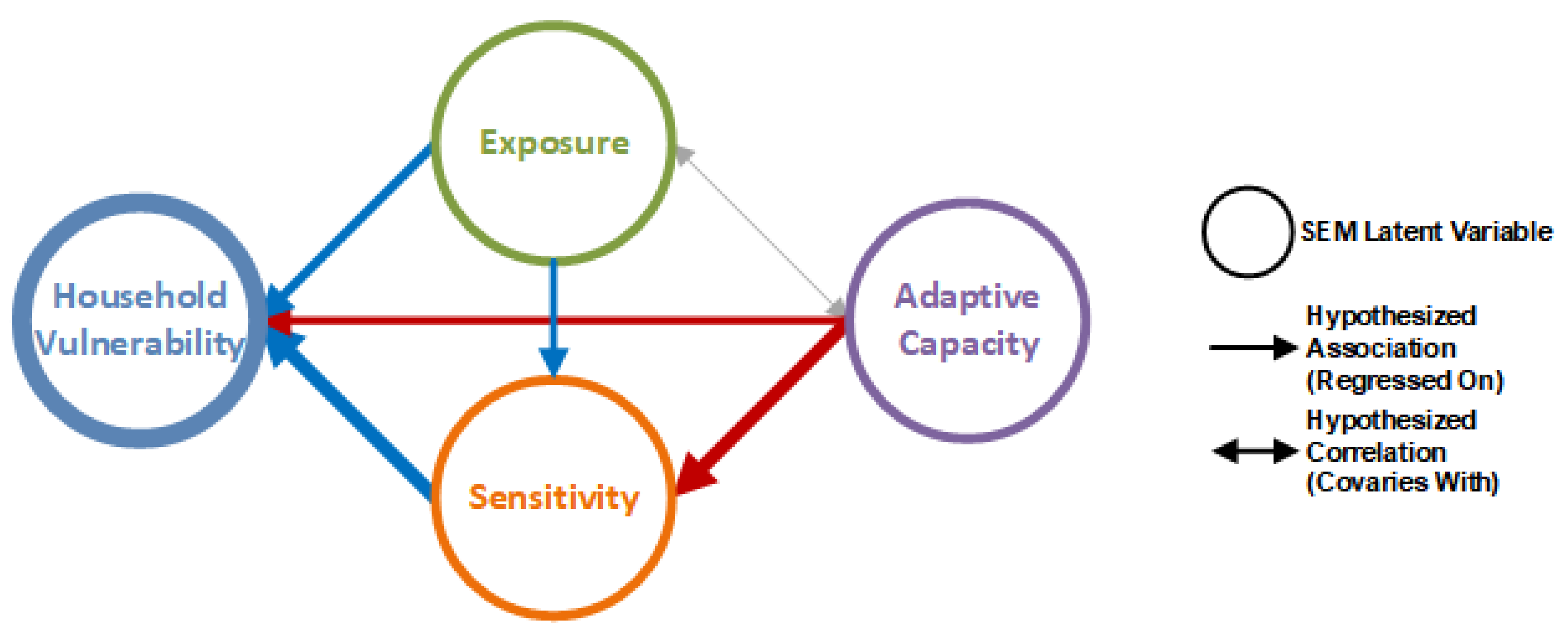
The model diagram in Figure 2 identifies the direct and indirect pathways of exposure, sensitivity, and adaptive capacity that, taken together, compose vulnerability. For the purpose of a land system example, we posit (and illustrate below) that in a rural setting, dryland systems households are sensitive to variations in exposure (e.g., land uses and their dependence on precipitation or vegetative productivity). The outcomes of these land uses in terms of agricultural products and amount of resources gathered (sensitivities) will be mediated by a household’s dependence on agricultural, livestock production, and natural resource gathering. That dependence may vary with the household’s adaptive capacity, or the other resources a household may rely on outside and in conjunction with the land function system. Thus, there are direct pathways or hypothesized associations between vulnerability and the other three components of the structural model. We also assume that an indirect effect on vulnerability exists from adaptive capacity and exposure through their combined effects with sensitivity (Figure 2). The proposed model, as a framework for vulnerability analyses, implies that the structural relationships should reflect the hypothesized pathways of dependence between latent and measured characteristics of vulnerability.
2.2. The Measurement Model
Assuming the structural model captures the nature of vulnerability in the system to an exposure of interest, the next step is to specify the measurement model for the structural components of the SEM. The specification of the model is a critical step since it is through this process that we are translating a proposed theory into a quantifiable framework, and defining what aspects of household vulnerability we are assessing. By fitting an SEM and its hypothesized dependence structure to measured indicator data, we determine whether our theoretical model will reflect the findings when the model is fitted with observed or measured data. We are arguing that the vulnerability framework consists of directly unmeasurable, latent aspects of the household (vulnerability, sensitivity, exposure, and adaptive capacity), that are often seen as aggregates of multiple household factors. In order to operationalize this framework, we must find measurable proxies or “indicators” that strongly correlate with these latent characteristics, and importantly, can be quantified at the household level.
In our proposed SEM approach to quantifying household vulnerability, measured indicator variables capture quantifiable information about the latent characteristics. With an identified model specification, these indicators are measured through empirical approaches and are assumed to be “predicted” by the unmeasurable, latent household characteristics (i.e., circles). These quantifiable features can be collected at the household level using combinations of household surveys, interviews, remote sensing, etc., and might be the outcomes of a mixed methods approach. In practice, the measures could be continuous or discrete, but are assumed to be quantifiable and relatable within and between structural components under assumptions of multivariate normality (though these assumptions might be relaxed when fitting the model with varying algorithms) [47,48,49,50].
However, the pre-specification is critical within an SEM approach once a combination of indicators representing the core, theoretical features of the conceptual framework are chosen. The principle of pre-specification, well known in psychology and other sciences, is considered to be a practice to improve reproducibility and reduce the likelihood of “hypothesizing after the results are known.” [51]. SEM as a statistical technique is based on estimating the variance/covariance structures between both measured and unmeasured components. In the case of the vulnerability framework proposed, these might include many possible measurable items. It is therefore necessary to make an effort to pre-specify the indicators to be used, how they relate to the vulnerability being assessed, and how such items would be measured to satisfy the quantification and distributional assumptions of the statistical technique. This should be done prior to analyzing and ideally even collecting the indicator data. In non-experimental settings, and especially in land systems household survey data that is cross-sectional, this may be difficult or impractical. For example, responses may be conditioned on spurious assumptions of language, culture or systemic bias, or measure something unintended as a result of some externality. These might only be discovered after data collection, but by pre-specifying an analysis to fit a conceptual modeling framework like our proposed vulnerability model, with measured indicators and potential alternative specifications, the researcher might reduce the potential for “data snooping” and finding spurious associations due to chance alone.
3. Illustration from a Motivating, Agripastoral Context
3.1. The Kavango–Zambezi Transboundary Dryland System
We illustrate the application of using an SEM to model vulnerability by describing a particular land system context in which it may be applied. We then describe a vulnerability model that is pre-specified, and simulate a synthetic dataset with a correlation structure to test assumptions of power and indicator relationships.
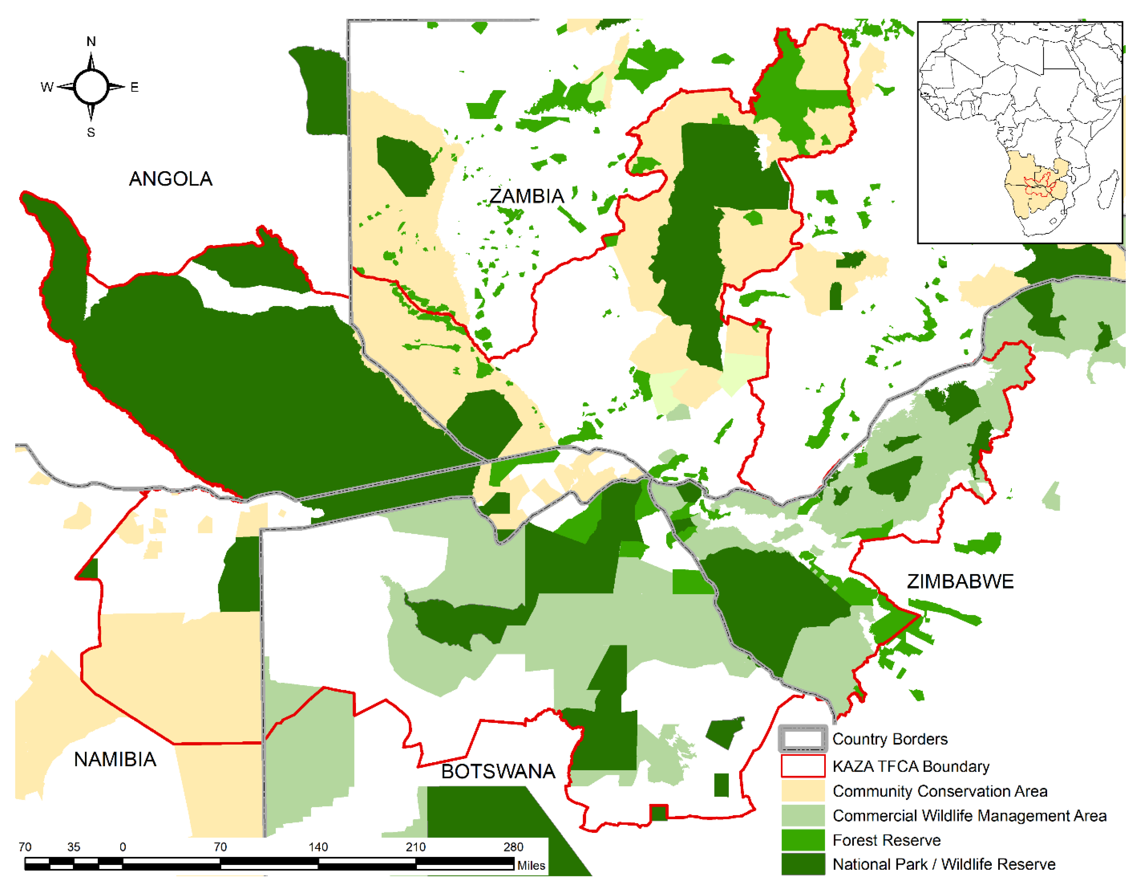
The land system context is the rural, dryland region within the Kavango–Zambezi Transfrontier Conservation Area (KAZA-TFCA) of Southern Africa (Figure 3). The system represents significant variation along livelihood, political, and biophysical dimensions. Spanning parts of Angola, Namibia, Botswana, Zambia, and Zimbabwe (~520,000 km2), the area has one of the largest elephant populations in the world and includes 36 protected areas interspersed with communal and private lands ([52]). It is also home to an estimated 2.3 million people in 2019 [53]. Excluding cities, the highest population densities are near main transport arteries, including rivers and roads, creating challenging management efforts for human-wildlife relations.
The KAZA_TFCA system is exemplary of how multi-level management differentially impacts these landscape dimensions, through underlying systems processes. The region includes open woodland, scrub and grasslands, characteristic of a heterogeneous semi-arid savanna [54,55,56]. Spanning a mean annual rainfall gradient of 400–1000 mm, the semi-arid savanna vegetation cover follows the gradient of an increasingly woody component with increasing mean annual rainfall [57]. However, that broad trend is disrupted by other mitigating factors such as fire and land management initiatives, grazing by wildlife and livestock, and soil-nutrient characteristics [58,59,60,61].
KAZA-TFCA is a varied landscape, both in terms of the land use and land cover but also with respect to governance. While national policies and community zoning initiatives influence broader patterns of vegetation heterogeneity, household land use decisions help shape the gradient of grass–shrub–tree for localized areas. The potential disconnects between the local level land use decisions and regional level zoning and resource use allocation is an important piece to understanding the KAZA-TFCA system as household vulnerability is variably affected by regional level zoning and land use policy. This is because there are multiple levels of management, some of which are working collectively towards common goals, and often geared toward a balance of conservation and development objectives. These goals are centered on the tourism industry, which is a substantial economic engine in the region. Engagement in the tourism sector provides one potential livelihood strategy to diversify and reduce the dependence on smallholder cropping. However, that alternative strategy is not accessible to all households in KAZA-TFCA leading to disparity and inconsistencies between development efforts directed at vulnerable households and regional level conservation initiatives.
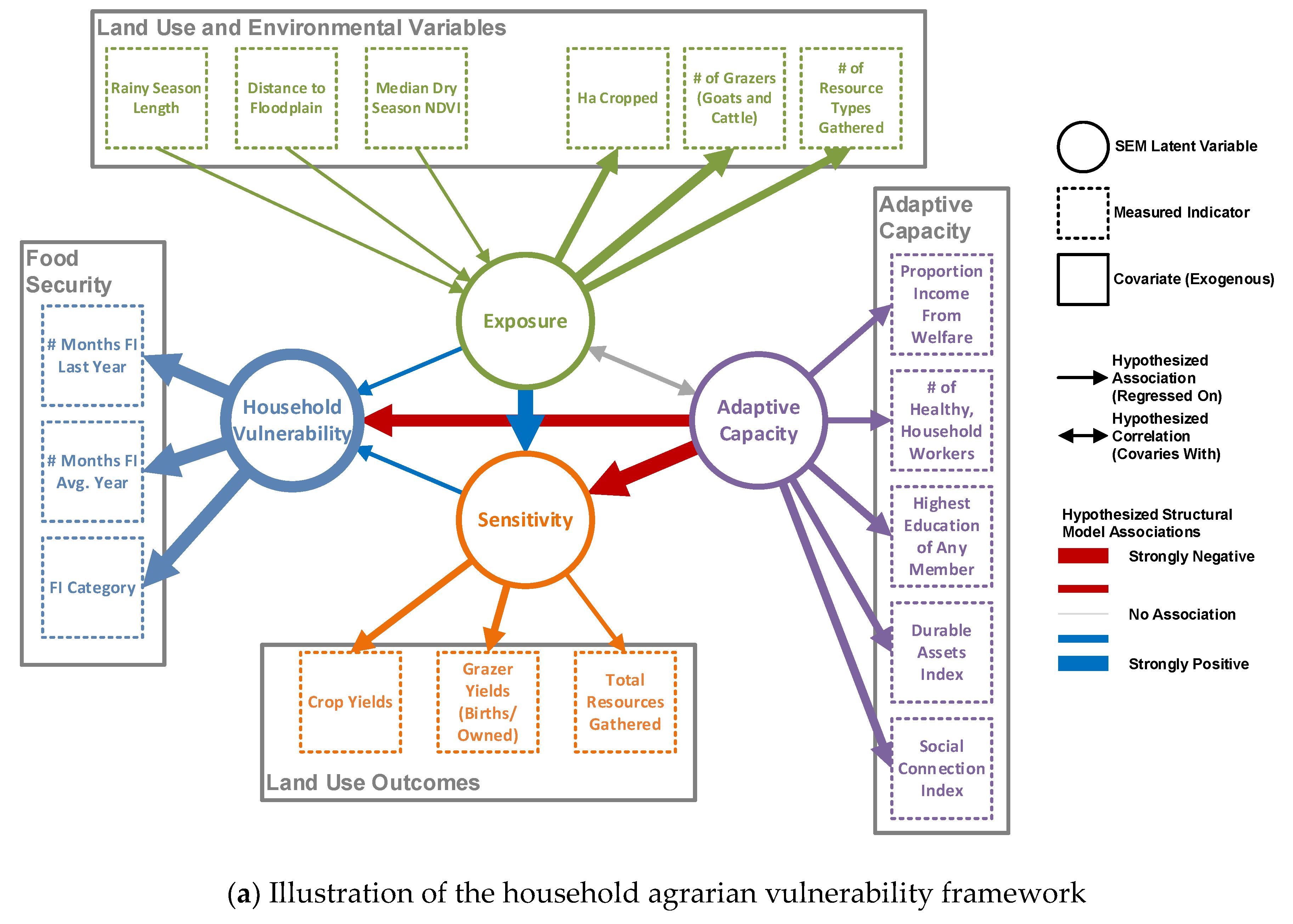
In conceptualizing the KAZA-TFCA system, we contend that household vulnerability, defined by food security with respect to land function, is captured through the combined influence of exposure, sensitivity, and adaptive capacity (Figure 4a). In simulation, we represent a typical household as primarily reliant on rain-fed crop production in the semiarid environment. Vulnerability as a latent, household characteristic is predictive of measured indicators that relate to food security. Vulnerability, as defined by food security, is linked to land use and environmental conditions of exposure. These exposure indicators include hectares cropped, number of grazers and the number of total resource types gathered. There is also a set of exogenous exposure predictors that inform the exposure in the system that represent proxies for the biophysical constraints that influence land uses (Figure 4a). In our simulated model, these variables are rainy season length, flooding, and dry season vegetation productivity, three variables that capture landscape functions tied to agricultural and livestock activities.
The sensitivity of a household to exposure may then relate closely to those environmental variables, representing outcomes of different land use activities. In this case, we chose proportion of crops produced that are sold, proportion of goods that are gathered and then sold (i.e., resources), and livestock yield. The mitigating influence of adaptive capacity captures how households variably adapt to stressors through accessing different forms of capital assets (e.g., financial, human, natural, physical, social). This realization allows us to explicitly consider human agency and diversity in behavior (i.e., adaptive response). Those capital assets capture the range of livelihood resources available to a household, especially in a rural context [22,62,63]. By extension, the capital assets provide a structure to assess the ability of those capitals—either individually [64] or collectively [65,66]—to provide a household with a buffer against shocks and unplanned change [34]. We include a set of indicators that represent financial, human, social and physical capitals that we feel collectively characterize a household’s ability to diversify and adapt. Natural capital is intrinsic to elements of exposure, sensitivity, and adaptive capacity due to the fundamental reliance on the environment; we therefore do not attempt to assign natural capital to specific measured variables but rather acknowledge its association with many model components that we measure variably.
For the KAZA-TFCA context, we assume that all indicators are measured at the household level. In the model, these directly relate to household vulnerability as they co-vary. In other contexts, and under similar assumptions as we propose with the SEM, approaches such as multilevel statistical models may also be effectively used to evaluate household vulnerability as a function of predictors existing at various levels or at different spatial or temporal scales. These approaches would also come with inherent tradeoffs (e.g., [67,68]). We discuss these considerations in Section 4 in the context of interventions for testing management and policy decisions specific to the conservation and development initiative that are paramount in regions such as KAZA-TFCA.
3.2. Testing Assumptions and Simulating Hypothesized Outcomes
To operationalize vulnerability, the simulation exercise illustrated for the KAZA-TFCA region is a useful tool to assess whether different model specifications, and their resulting potential data realizations, fit our hypothesized, intuitive, or expected relationships between parts of the system. Furthermore, we can assess the strength of hypothesized correlations in conjunction with basic power analyses for survey size and model complexity exploration. This is important, especially in an SEM modeling context, as alternative models should be explored (different indicators used and varying pathways defined) prior to bringing that specification to the data. It is often trivial to modify the model design to fit some aspect of the data a posteriori, which may be undesirable unless pure prediction is the goal.
For the purpose of simulation, we estimated from systematic testing that a sample of 600 household observations was the sample size requirement to fit the SEM to the KAZA-TFCA system [69]. The sample size also represents an approximately adequate sample for capturing household dynamics in community-based areas of KAZA-TFCA using a model of this complexity but with potentially weak correlations between components, which is typical in social data contexts [40,70]. Selected indicators are detailed in Table 1, and correspond to those in the hypothetical vulnerability model in Figure 4a. These indicators represent socio-economic information for rural households and biophysical characteristics for a semi-arid, savanna landscape of KAZA-TFCA (Figure 3a) [71,72]). Most households are located in sparsely settled, remote villages where reliance on natural resources is high, integration in the cash economy is low, and livelihoods are based on subsistence crop and livestock production.
Standardized coefficient estimations based on simulated data from the structural relationship in Figure 2 are presented in Figure 4a. The color and width of arrows reflect the correlation structure imposed by our hypothesized indicators. Using such a simulation and hypotheses about the strengths of correlated indicators provides insight into how our sampling frame responds to our hypothesized model specification. The illustration suggests the strength of association (negative is red, positive is blue) that a measured variable has on the different latent characteristics and reflects the correlation and covariance of both measured and unmeasured (estimated) components of the model. The colored arrows point in the direction of dependency or “regressed-on” dependence relationships while grey arrows represent correlative relationships. The thickness of an arrow represents the relative strength of a path relationship.
Located in the supplemental text (S1) is the code and the quantitative correlation/covariance structure produced by the hypothesized model. The fit of the model against the simulated data can be used in conjunction with variable household survey sizes, and various parametric permutations for indicator measures to design the survey and sampling frame. Most importantly, different generative models can be used to simulate data that can be fit to the multiple alternative model and indicator designs. This feature of the SEM framework and formulation allows researchers to explore how conclusions based on model fit to real data under “wrong” or “incorrect” theoretical relationships might change conclusions about the strength of the theory or the model.
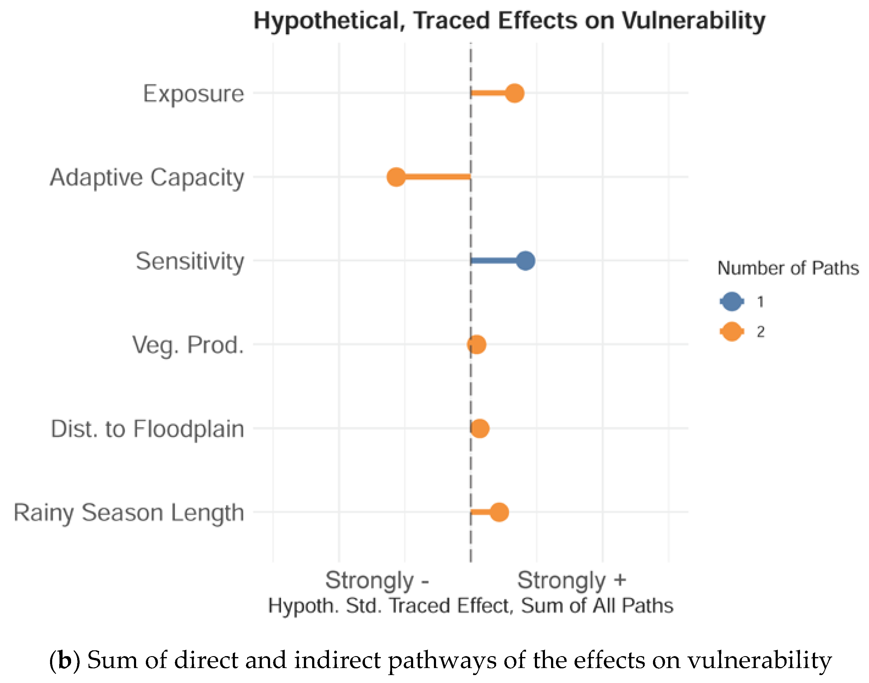
Additionally, we summarize the hypothesized "total path" effect from a model fit to the simulated data (i.e., the sum of total direct and indirect pathways) (Figure 4b). This shows the relative path strengths (S1) we might expect between the respective latent components. The "total path" effect describes how household exposure to land system factors influences household vulnerability as mediated by its sensitivity and mitigated by adaptive capacity. The arrows point in the direction of dependency or “regressed-on” relationships, meaning, for example, that the blue arrows pointing from exposure and sensitivity to vulnerability (Figure 4a) represent positive, direct pathways for how exposure and sensitivity relate to vulnerability. In contrast, adaptive capacity has two pathways identified with red arrows (Figure 4a), one with a direct path to vulnerability (thinner, red line) and the other, a thicker, red line drawn to sensitivity to indicate that the effect of adaptive capacity on vulnerability will be a product not only of the predictive capacity of adaptive capacity alone, but also as it relates to sensitivity. To trace the total path effect on vulnerability for each covariate, Figure 4b notes the number of potential pathways and whether those path effects are positive or negative. In this case, higher exposure will have a positive effect on vulnerability. Furthermore, while sensitivity is also associated with an increase in vulnerability, it is a weaker relationship. However, as adaptive capacity goes down (which negatively influences vulnerability), sensitivity will go up. We also hypothesize that the external environmental components and their variation across households have a small but statistically significant effect on exposure and therefore vulnerability, and are important to control for when assessing the other components and their relationships.
4. Discussion
4.1. Vulnerability in the Agripastoral Context
In presenting a hypothetical structural equation model that treats household vulnerability as a composite of exposure, sensitivity, and adaptive capacity, we acknowledge that methodologically and conceptually we are fusing two established approaches. However, in choosing to represent these latent constructs, especially in terms of exposure and sensitivity, as the intersection of land use and its outcomes, we argue that this approach can be situated firmly within land systems contexts. Doing it in this way better operationalizes such theory and facilitates better decision-making around states and change in household vulnerability and land management. While pooling such land functions within households across multiple land uses may not be appropriate in contexts outside of the KAZA-TFCA case presented as illustration, the intersectional aspect of the theory and model choices made can be tailored to address specific aspects of land functions as they relate to household vulnerability in other contexts.
4.2. Introducing Interventions, Assessing Leverage Points
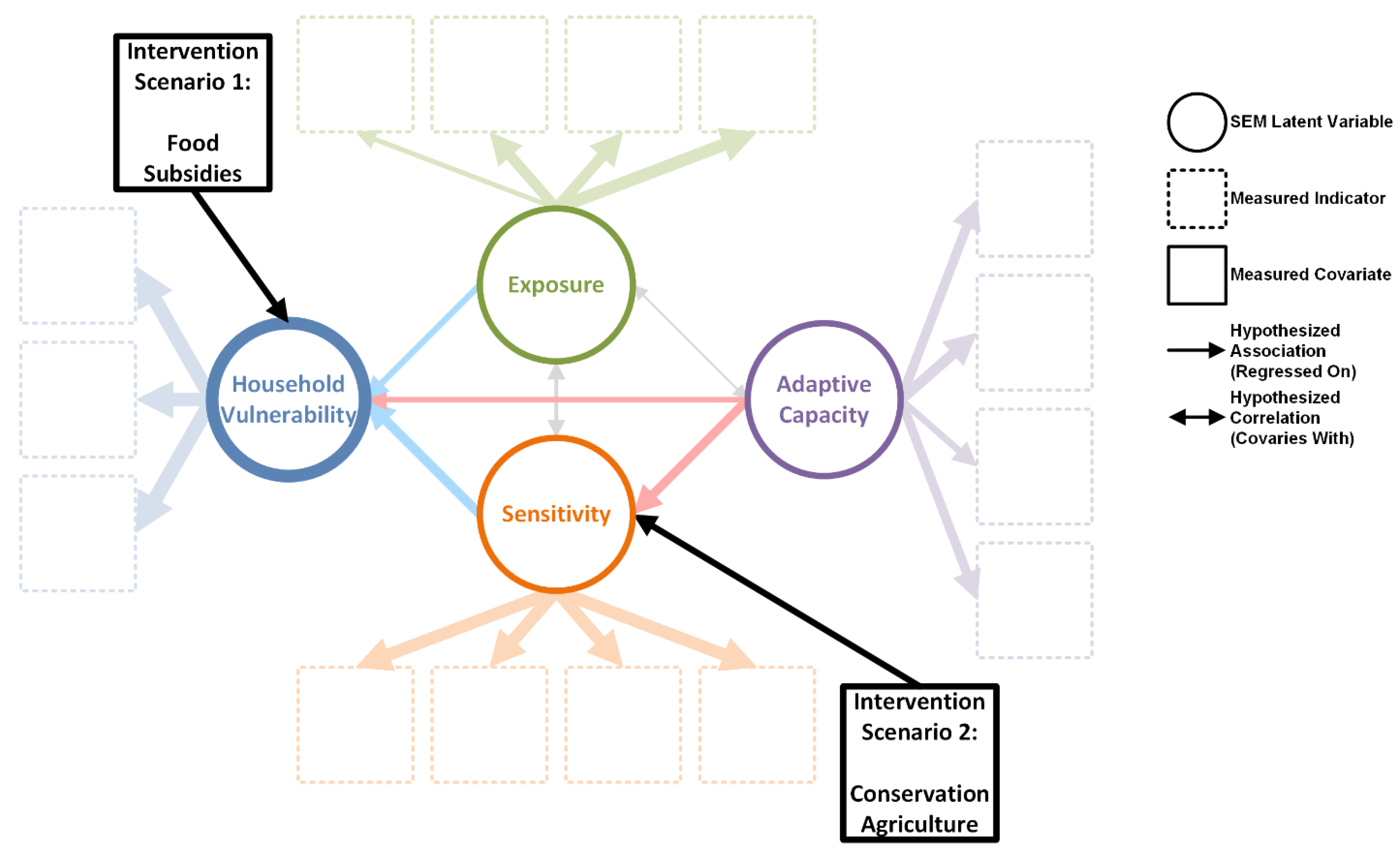
Additionally, the proposed approach provides a systematic way to test policy and management initiatives aimed at alleviating household vulnerability. The flexibility of the SEM approach provides a means of assessment in how policy interventions may impact system dynamics. Those impacts may be tested a priori to an intervention in order to identify best options for inserting leverage points without large social or financial risk. Alternatively, post-intervention impacts can be measured through the strength of observed relationships based on a follow-up assessment. For example, additional mediating variables that might impact either the unmeasured, latent characteristics or individual measured covariates (e.g., drought relief in the form of food subsidies, livelihood support in the form of agricultural techniques) can be included in the model. If an intervention was designed to target any one component of the system and applied to a subset of households, it could be included as another variable in the model to estimate its influence while holding constant the structural relationships between vulnerability components. Most importantly, values of unmeasured, latent variables can be estimated from a model fit to measure indicators and covariates. In similar ways to vulnerability indices, these estimates of latent features can be compared across households. Since the structural parts of the fitted model and its coefficients can be interpreted as one might a traditional linear model, the impacts of potential interventions aimed at changing a household’s sensitivity or adaptive capacity can be assessed. The effect of an intervention aiming to change a household’s state in any one latent characteristic (e.g., moving a household from poor to exceptional adaptive capacity), can be estimated by applying the coefficients through all connected pathways and then estimating the potential change in that household’s latent vulnerability score. Changes in these latent characteristics can then also be used to estimate changes in measured indicators.
Past interventions might also be added to the model to test effects of policies targeting specific indicators, or more broadly an entire latent characteristic. Using the KAZA-TFCA food security example, an intervention such as the provision of food subsidies to alleviate hunger directly (a direct impact to the latent characteristic of vulnerability) or the adoption of conservation agriculture as a means to alleviate sensitivity to exposure introduced by climate variation (Figure 5), we might gain quantitative insight into which interventions to prioritize. To accomplish this quantitatively, we can simulate the outcomes of a particular intervention on the estimated values of a latent variable, as translated through the predicted system of path effects.
Food subsidies (Scenario 1) highlights a short-term (i.e., more immediate) targeted effort towards an indicator of the latent construct vulnerability. Specifically, food rations are distributed to individual households in communities; the interventions are typically determined at the national level, so subsidies may reach some KAZA-TFCA communities but not others. We argue that the temporality of an intervention targeted at the latent construct of vulnerability provides only short-term relief to a household. While the intervention could be highly impactful towards initial hunger and mortality of a household, the long-term sustainability of that household, the resilience towards future situations of similar context, does not get addressed with this type of intervention. In contrast, conservation agriculture (Scenario 2), the intercropping of nitrogen-fixing crops between rows of typically farmed maize or sorghum crops, aimed towards the latent construct of sensitivity, has the potential to introduce a longer-term adaptive intervention.
Be estimating the effects of a hypothesized intervention, we assume that the intervention in question is going to target a structural component in the model. Such an intervention would therefore translate, according to the strength of the correlations with the measured, indicator variables, to outcomes in those variables. Thus, it is important to consider the temporal aspect of a given intervention on the correlative strengths that connect the measured and structured parts of the vulnerability model. Any intervention will influence the strength of association between measured indicators and their latent constructs, but the relationships will change based on which latent construct is targeted (e.g., vulnerability, sensitivity, or adaptive capacity) and the timeframe needed to observe a change in the overall vulnerability model. A vulnerable condition is not static but oftentimes we are forced to assess and measure that state as a snapshot in time [73]. These types of longitudinal impacts, or studies of vulnerability across time might be well served by the proposed conceptual framing. Recent studies emphasize the importance of new methodologies to generate insight into longitudinal studies of vulnerability and associated features of these systems have been proposed [74]. We believe that the considerations and advances in incorporating pre–post impact assessments, trend analyses, and longitudinal data in general can be incorporated into the SEM-based framework. In its most general case, however, we are most interested in the combined effect on vulnerability and its indicators that results from any single intervention that affects a household’s adaptive capacity or sensitivity. The impact of such an intervention on the latent and measured outcomes of household vulnerability may include not just the direct paths linking these structural components, but also the indirect paths, such as the two pathways between adaptive capacity and vulnerability (direct and the one through sensitivity) (Figure 4a,b).
A challenge with the proposed method is the need to correctly specify and evaluate candidate model structures that reflect potential underlying causal and correlative associations [40,75]. The model described in Figure 2 is just one such specification, and forms the basis of a strong understanding of the SES based on previous work in the region, the current literature, and a theoretical underpinning of how various livelihood capital components accentuate or mediate interactions with biophysical features in agricultural areas to create or mitigate household vulnerability.
Another overriding consideration in any social–ecological model is the scales of interest and the data being used. Though the indicators must be measured at the household level, some indicators, especially for exposure in the climate context, may only vary across coarser, regional extents [58,59]. If this is the case, then the scale of data collection must match the variability in the indicators used, and the type of vulnerability being specified must reflect those scalar considerations. Thus, depending on the scale of assessment (e.g., household, community, region), the multi-scale dynamics of measured indicators needs to be explicitly accounted for in model development. How researchers address these scalar issues may depend greatly on the range of relevant temporal and spatial scales, and how these relate to the latent or structural components of the model. Researchers must ask whether those structural components, if they were measurable, adequately predict those measured indicators at the scale of measurement. Additionally, we must address whether the correlations and covariance between measured components are the result of processes effecting pattern, or alternatively if they might be induced by such things as modifiable areal unit issues, or temporal periodicity. These types of issues are inherent to spatiotemporal analyses, and to the extent these data are included in vulnerability analyses, they must be addressed within the proposed framework as well.
Another noteworthy aspect to the SEM approach is the need for large sample sizes. In designing the SEM (Figure 4a), a minimum of 68 parameters is needed (covariance between indicators is not shown in Figure 3a for clarity), and undertaking a basic power analysis using the hypothesized correlation structure and strength of associations among components, simulated data indicate that these associations could be roughly estimated using between 250 and 600 individual household observations. While a proposed sample size of 1000 household surveys should be adequate, community-level differences or country-specific features that would involve partitioning data into sub-groups will require an increased sample size to ensure unbiased and accurate estimates of the conditional associations.
Lastly, it is also important to note that the model form presented is not the only potential configuration of the relationships between vulnerability, exposure, sensitivity and adaptive capacity, nor the only statistical model that might be applied. Other types of approaches have been explored in social–ecological systems [30,37,76,77]. For example, Pandey et al. operationalize vulnerability by a set of indices that assess both vulnerability and the ability to adapt to certain conditions. They measure a set of indicators for three dimensions of vulnerability (exposure, sensitivity, adaptive capacity) with specific indicators divided into various capitals (human, natural, physical, social, financial). To create indices, they aggregate indicators of respective vulnerability components with a balanced weighted average approach [77]. Their approach provides a level of specificity necessary to identify nuances in livelihood coping strategies and a quantifiable means for examining differences in household vulnerability. Metcalf et al. (2015) also employ a livelihoods framework coupled with a vulnerability framework but rely on secondary datasets and a representative set of surveys rather than direct household information for their analysis. Their assessment is focused at the community level and applies the codependency framework [30,76] which links separate vulnerability models for the ecosystem and socioeconomic components of a system.
5. Conclusions
We present a novel approach linking theory to empirical estimation to policy, coupling a conceptual framework of household vulnerability to a statistical model in a land systems context. Following the application of field-based observations from a given system, our approach allows for the prediction and assessment of the impact of, for example, policy decisions to allocate funds for food subsidies or implementing a longer-term ground strategy aimed at conservation agricultural initiatives (as in Figure 4a). Additionally, the model may be used as a predictive tool for the latent components of vulnerability, sensitivity, exposure and adaptive capacity in response to land system changes. The model is also useful to assess the impacts after an intervention and identify the strength of relationships post-intervention.
The power of an empirical model formulation based on correlation and covariance such as the one that structural equation modeling provides, is that the paths between components, as quantified in Figure 4a, can provide insight into how a policy or programmatic intervention may act as a system lever to directly affect indicators of household or community vulnerability. These pathways represent opportunities for policy and associated interventions at multiple levels to more appropriately target actions to affect positive outcomes. While the framework provides an interesting design for engaging public stakeholders in discussions about community vulnerability and adaptive response (in this particular case, to climate change), the relationships measured are as independent correlative associations with no direct means of intervention assessment. These cases demonstrate the importance of combining the theoretical frameworks of livelihoods and vulnerability in a quantifiable manner for examining SES dynamics at either a household or community level. We take that one step further by presenting a quantifiable approach that assesses all system components otherwise difficult to directly measure (i.e., vulnerability, adaptive capacity, sensitivity, exposure) by measuring potential underlying causal and correlative associations of different indicator variables. However, regardless of approach, the design of measuring vulnerability must be flexible enough to accommodate various SES structures [8].
We used examples from a dryland African SES where livelihoods are highly dependent on local natural resources to illustrate a coupled theoretical and applied vulnerability approach. This approach allows us to explain the variability in measured indicators across the different households surveyed and describe, at the household level, how independent households vary across the region. Further, we can also estimate the degree to which a latent characteristic of exposure, adaptive capacity or sensitivity relate to vulnerability at the household level. Importantly, the flexibility of the model allows adjustments to examine alternative hypotheses by adjusting the number or type of indicator informing any of the four latent constructs in the SEM. We provide a representative agrarian rural household model for purposes of explaining how the process of framework-to-empirical testing happens.
Supplementary Materials
The data in the paper were simulated and the code to generate those simulations is available online at https://susy.mdpi.com/user/manuscripts/displayFile/5b77a4e63f778a1d7d016873adaf4b86?v=7625481.
Author Contributions
A.E.G., F.R.S., N.G.P., J.H., L.C., and J.S. theoretically conceptualized and designed this study. The simulation model was built and tested by F.R.S. with input from other co-authors. Funding acquisition was done by A.E.G., F.R.S., N.G.P., J.H. and L.C. A.E.G. drafted the manuscript and all authors contributed to the final version.
Funding
This research is supported by the United States National Science Foundation (NSF) (#1560700) entitled, “Land Systems Dynamics, Vulnerability and Adaptation in a Transfrontier Conservation Area.” (https://www.nsf.gov/awardsearch/showAward?AWD_ID=1560700).
Acknowledgments
Thank you to the communities of Zambezi Region, Namibia and Chobe Enclave in Botswana. Without their willingness to engage in the research study, this type of work would not be possible. We also thank the KAZA-TFCA Secretariat, the University of Namibia, the Integrated Rural Development and Nature Conservation, the Department of National Parks and Wildlife in Zambia, and Dr. Patricia Mupeta-Muyamwa for their insight, collaboration and support of our work. We also thank the external reviewers for the thoughtful and useful critiques for improving the final version of this paper.
Conflicts of Interest
The authors declare no conflict of interest. The funders had no role in the design of the study; in the collection, analyses, or interpretation of data; in the writing of the manuscript, or in the decision to publish the results.
References
- Verburg, P.H.; Erb, K.H.; Mertz, O.; Espindola, G. Land system science: Between global challenges and local realities. Curr. Opin. Environ. Sustain. 2013, 5, 433–437. [Google Scholar] [CrossRef] [PubMed]
- Verburg, P.H.; Dearing, J.A.; Dyke, J.G.; Leeuw, S.; van der Seitzinger, S.; Steffen, W.; Syvitski, J. Methods and approaches to modelling the Anthropocene. Glob. Environ. Chang. 2016, 39, 328–340. [Google Scholar] [CrossRef] [Green Version]
- Seppelt, R.; Lautenbach, S.; Volk, M. Identifying trade-offs between ecosystem services, land use, and biodiversity: A plea for combining scenario analysis and optimization on different spatial scales. Curr. Opin. Environ. Sustain. 2013, 55, 458–463. [Google Scholar] [CrossRef]
- Nielsen, J.Ø.; de Bremond, A.; Roy Chowdhury, R.; Friis, C.; Metternicht, G.; Meyfroidt, P.; Munroe, D.; Pascual, U.; Thomson, A. Toward a normative land systems science. Curr. Opin. Environ. Sustain. 2019, 38, 1–6. [Google Scholar] [CrossRef]
- Luers, A.L.; Lobell, D.B.; Sklar, L.S.; Addams, C.L.; Matson, P.A. A method for quantifying vulnerability, applied to the agricultural system of the Yaqui Valley, Mexico. Glob. Environ. Chang. 2003, 13, 255–267. [Google Scholar] [CrossRef]
- Turner, B.L.; Matson, P.A.; McCarthy, J.J.; Corell, R.W.; Christensen, L.; Eckley, N.; Hovelsrud-Broda, G.K.; Kasperson, J.X.; Kasperson, R.E.; Luers, A.; et al. Illustrating the coupled human-environment system for vulnerability analysis: Three case studies. Proc. Natl. Acad. Sci. USA 2003, 100, 8080–8085. [Google Scholar] [CrossRef] [PubMed]
- O’Brien, K.; Leichenko, R.; Kelkar, U.; Venema, H.; Aandahl, G.; Tompkins, H.; Javed, A.; Bhadwal, S.; Barg, S.; Nygaard, L.; et al. Mapping vulnerability to multiple stressors: Climate change and globalization in India. Glob. Environ. Chang. 2004, 14, 303–313. [Google Scholar] [CrossRef]
- Adger, W.N. Vulnerability. Glob. Environ. Chang. 2006, 16, 268–281. [Google Scholar] [CrossRef]
- Eakin, H.; Luers, A.L. Assessing the vulnerability of social-environmental systems. Annu. Rev. Environ. Resour. 2006, 31, 365–394. [Google Scholar] [CrossRef]
- Hinkel, J. Indicators of vulnerability and adaptive capacity: Towards a clarification of the science-policy interface. Glob. Environ. Chang. 2011, 21, 198–208. [Google Scholar] [CrossRef]
- Birkmann, J.; Cardona, O.D.; Carreño, M.L.; Barbat, A.H.; Pelling, M.; Schneiderbauer, S.; Kienberger, S.; Keiler, M.; Alexander, D.; Zeil, P.; et al. Framing vulnerability, risk and societal responses: The MOVE framework. Nat. Hazards 2013, 67, 193–211. [Google Scholar] [CrossRef]
- Blaikie, P.; Terry, C.; Ian, D.; Ben, W. At Risk: Natural hazards, people’s vulnerability, and disasters. Hum. Ecol. 1996, 24, 141–145. [Google Scholar]
- Kasperson, R.E.; Kasperson, J.X. Climate Change, Vulnerability and Social Justice; Stockholm Environment Institute: Stockholm, Sweden, 2001; Volume 26, pp. 1–18. [Google Scholar]
- Turner, B.L.; Kasperson, R.E.; Matson, P.A.; McCarthy, J.J.; Corell, R.W.; Christensen, L.; Eckley, N.; Kasperson, J.X.; Luers, A.; Martello, M.L.; et al. A framework for vulnerability analysis in sustainability science. Proc. Natl. Acad. Sci. USA 2003, 100, 8074–8079. [Google Scholar] [CrossRef] [PubMed] [Green Version]
- Cutter, S.L.; Boruff, B.J.; Shirley, W.L. Social vulnerability to environmental hazards. Soc. Sci. Q. 2003, 84, 242–261. [Google Scholar] [CrossRef]
- Leichenko, R.; O’Brien, K. Environmental Change and Globalization; Oxford University Press: Oxford, UK, 2008; ISBN 9780195177329. [Google Scholar]
- Young, O.R.; Berkhout, F.; Gallopin, G.C.; Janssen, M.A.; Ostrom, E.; van der Leeuw, S. The globalization of socio-ecological systems: An agenda for scientific research. Glob. Environ. Chang. 2006, 16, 304–316. [Google Scholar] [CrossRef]
- Ostrom, E. A diagnostic approach for going beyond panaceas. Proc. Natl. Acad. Sci. USA 2007, 104, 15181–15187. [Google Scholar] [CrossRef] [PubMed] [Green Version]
- Costa, L.; Kropp, J.P. Linking components of vulnerability in theoretic frameworks and case studies. Sustain. Sci. 2013, 8, 1–9. [Google Scholar] [CrossRef]
- Wisner, B.; Luce, H.R. Disaster vulnerability: Scale, power and daily life. GeoJournal 1993, 30, 127–140. [Google Scholar] [CrossRef]
- Gunderson, L. Ecological and human community resilience in response to natural disasters. Ecol. Soc. 2010, 15, 29. [Google Scholar] [CrossRef]
- Sen, A. Concepts of Poverty. In Poverty and Famines: An Essay on Entitlement and Deprivation; Oxford University Press: Oxford, UK, 1981; ISBN 9780198284635. [Google Scholar]
- Scoones, I. Sustainable rural livelihoods: A framework for analysis. IDS Work. Pap. 1998, 72, 22. [Google Scholar]
- Peduzzi, P.; Dao, H.; Herold, C.; Mouton, F. Assessing global exposure and vulnerability towards natural hazards: The disaster risk index. Nat. Hazards Earth Syst. Sci. 2009, 9, 1149–1159. [Google Scholar] [CrossRef]
- Thomalla, F.; Downing, T.; Spanger-Siegfried, E.; Han, G.; Rockström, J. Reducing hazard vulnerability: Towards a common approach between disaster risk reduction and climate adaptation. Disasters 2006, 30, 39–48. [Google Scholar] [CrossRef] [PubMed]
- IPCC TAR IPCC. Third Assessment Report (TAR); IPCC: Geneva, Switzerland, 2001; p. 995. [Google Scholar]
- IPCC IPCC. Fourth Assessment Report (AR4); IPCC: Geneva, Switzerland, 2007; Volume 1, p. 976. [Google Scholar]
- IPCC IPCC. Fifth Assessment Report (AR5); IPCC: Geneva, Switzerland, 2013; pp. 10–12. [Google Scholar]
- Wisner, B.; Blaikie, P.; Cannon, T.; Davis, I. At Risk: Natural Hazards, People’ s Vulnerability and Disasters, 2nd ed.; Routledge: Abingdon, UK, 2003; p. 134. [Google Scholar]
- Metcalf, S.J.; van Putten, E.I.; Frusher, S.; Marshall, N.A.; Tull, M.; Caputi, N.; Haward, M.; Hobday, A.J.; Holbrook, N.J.; Jennings, S.M.; et al. Measuring the vulnerability of marine social-ecological systems: A prerequisite for the identification of climate change adaptations. Ecol. Soc. 2015, 20, 35. [Google Scholar] [CrossRef]
- Turner, B.L.; Janetos, A.C.; Verburg, P.H.; Murray, A.T. Land system architecture: Using land systems to adapt and mitigate global environmental change. Glob. Environ. Chang. 2013, 23, 395–397. [Google Scholar] [CrossRef]
- Fraser, E.D.G.; Dougill, A.J.; Hubacek, K.; Quinn, C.H.; Sendzimir, J.; Termansen, M. Assessing vulnerability to climate change in dryland livelihood systems: Conceptual challenges and interdisciplinary solutions. Ecol. Soc. 2011, 16, 1. [Google Scholar] [CrossRef]
- Walker, B.; Carpenter, S.; Anderies, J.; Abel, N.; Cumming, G.; Janssen, M.; Lebel, L.; Norberg, J.; Peterson, G.D.; Pritchard, R. Resilience management in social-ecological systems: A working hypothesis for a participatory approach. Ecol. Soc. 2002, 6, 14. [Google Scholar] [CrossRef]
- Tanner, T.; Lewis, D.; Wrathall, D.; Bronen, R.; Cradock-Henry, N.; Huq, S.; Lawless, C.; Nawrotzki, R.; Prasad, V.; Rahman, M.A.; et al. Livelihood resilience in the face of climate change. Nat. Clim. Chang. 2014, 5, 23–26. [Google Scholar] [CrossRef]
- Leichenko, R.M.; O’Brien, K.L. The dynamics of rural vulnerability to global change: The case of southern Africa. Mitig. Adapt. Strateg. Glob. Chang. 2002, 7, 1–18. [Google Scholar] [CrossRef]
- Hoyle, R.H. Handbook of Structural Equation Modeling; Guilford Press: New York, NY, USA, 2012. [Google Scholar]
- Gerlitz, J.Y.; Macchi, M.; Brooks, N.; Pandey, R.; Banerjee, S.; Jha, S.K. The multidimensional livelihood vulnerability index–an instrument to measure livelihood vulnerability to change in the Hindu Kush Himalayas. Clim. Dev. 2017, 9, 124–140. [Google Scholar] [CrossRef]
- Asah, S.T. Empirical social-ecological system analysis: From theoretical framework to latent variable structural equation model. Environ. Manag. 2008, 42, 1077–1090. [Google Scholar] [CrossRef]
- Schumacker, R.E.; Lomax, R.G. A Beginner’s Guide to Structural Equation Modeling, 4th ed.; Routledge: New York, NY, USA, 2015. [Google Scholar]
- Kline, R.B. Principles and Practice of Structural Equation Modeling, 3rd ed.; Guilford Press: New York, NY, USA, 2011; ISBN 978-1-60623-877-6 978-1-60623-876-9. [Google Scholar]
- Lei, P.W.; Wu, Q. An NCME instructional module on: Introduction to structural equation modeling: Issues and practical considerations. Educ. Meas. Issues Pract. 2007, 26, 33–43. [Google Scholar] [CrossRef]
- Roberts, D. The role of households in sustaining rural economies: A structural path analysis. Eur. Rev. Agric. Econ. 2005, 32, 393–420. [Google Scholar] [CrossRef]
- Zakour, M.J.; Gillespie, D.F. Community Disaster Vulnerability: Theory, Research, and Practice; Springer: Berlin, Germany, 2013; ISBN 978-1461457367. [Google Scholar]
- Dang, H.L.; Li, E.; Nuberg, I.; Bruwer, J. Understanding farmers’ adaptation intention to climate change: A structural equation modelling study in the Mekong Delta, Vietnam. Environ. Sci. Policy 2014, 41, 11–22. [Google Scholar] [CrossRef]
- Grootaert, C.; Kanbur, R.; Oh, G.T. The dynamics of welfare gains and losses: An African case study. J. Dev. Stud. 1997, 33, 635–657. [Google Scholar] [CrossRef]
- Brown, D.G.; Verburg, P.H.; Pontius, R.G.; Lange, M.D. Opportunities to improve impact, integration, and evaluation of land change models. Curr. Opin. Environ. Sustain. 2013, 5, 452–457. [Google Scholar] [CrossRef]
- Wirth, R.J.; Edwards, M.C. Item factor analysis: Current approaches and future directions. Psychol. Methods 2007, 12, 58. [Google Scholar] [CrossRef] [PubMed]
- Mîndrilă, D. Maximum likelihood (ML) and diagonally weighted least squares (DWLS) estimation procedures: A comparison of estimation bias with ordinal and multivariate non-normal data. Int. J. Digit. Soc. 2016, 1, 60–66. [Google Scholar] [CrossRef]
- Palomo, J.; Dunson, D.B.; Bollen, K. Bayesian structural equation modeling. In Handbook of Latent Variable and Related Models; Elsevier: Amsterdam, The Netherlands, 2007; ISBN 9780444520449. [Google Scholar]
- DiStefano, C. The impact of categorization with confirmatory factor analysis. Struct. Equ. Model. 2002, 9, 327–346. [Google Scholar] [CrossRef]
- Munafò, M.R.; Nosek, B.A.; Bishop, D.V.M.; Button, K.S.; Chambers, C.D.; Percie Du Sert, N.; Simonsohn, U.; Wagenmakers, E.J.; Ware, J.J.; Ioannidis, J.P.A. A manifesto for reproducible science. Nat. Hum. Behav. 2017, 1, 21. [Google Scholar] [CrossRef]
- Munthali, S.M.; Smart, N.; Siamudaala, V.; Mtsambiwa, M.; Harvie, E. Integration of ecological and socioeconomic factors in securing wildlife dispersal corridors in the Kavango-Zambezi transfrontier conservation area, Southern Africa. In Selected Studies in Biodiversity; Books on Demand: Norderstedt, Germany, 2018. [Google Scholar]
- WorldPop, Global High Resolution Population Denominators Project. Available online: https://www.worldpop.org/ (accessed on 2 July 2019).
- Gibbes, C.; Cassidy, L.; Hartter, J.; Southworth, J. The monitoring of land-cover change and management across gradient landscapes in Africa. In Human-Environment Interactions: Current and Future Directions; Springer: Dordrecht, The Netherlands, 2013; pp. 165–209. ISBN 9789400747807. [Google Scholar]
- Gaughan, A.E.; Waylen, P.R. Spatial and temporal precipitation variability in the Okavango-Kwando-Zambezi catchment, southern Africa. J. Arid Environ. 2012, 82, 19–30. [Google Scholar] [CrossRef]
- Pricope, N.G.; Binford, M.W. A spatio-temporal analysis of fire recurrence and extent for semi-arid savanna ecosystems in southern Africa using moderate-resolution satellite imagery. J. Environ. Manag. 2012, 100, 72–85. [Google Scholar] [CrossRef] [PubMed]
- Gaughan, A.E.; Stevens, F.R.; Gibbes, C.; Southworth, J.; Binford, M.W. Linking vegetation response to seasonal precipitation in the Okavango-Kwando-Zambezi catchment of southern Africa. Int. J. Remote Sens. 2012, 33, 6783–6804. [Google Scholar] [CrossRef]
- Archibald, S.; Scholes, R.J. Leaf green-up in a semi-arid African savanna—Separating tree and grass responses to environmental cues. J. Veg. Sci. 2007, 18, 583. [Google Scholar]
- Sankaran, M.; Hanan, N.P.; Scholes, R.J.; Ratnam, J.; Augustine, D.J.; Cade, B.S.; Gignoux, J.; Higgins, S.I.; Le Roux, X.; Ludwig, F.; et al. Determinants of woody cover in African savannas. Nature 2005, 438, 846. [Google Scholar] [CrossRef] [PubMed]
- Pricope, N.G.; Gaughan, A.E.; All, J.D.; Binford, M.W.; Rutina, L.P. Spatio-temporal analysis of vegetation dynamics in relation to shifting inundation and fire regimes: Disentangling environmental variability from land management decisions in a southern african transboundary watershed. Land 2015, 4, 627–655. [Google Scholar] [CrossRef]
- Cumming, D.H.M. Large Scale Conservation Planning and Priorities for the Kavango-Zambezi Transfrontier Conservation Area; Conservation International: Arlington, VA, USA, 2008. [Google Scholar]
- Carney, D.; Drinkwater, M.; Neefjes, K.; Rusinow, T.; Wanmali, S.; Singh, N. Livelihoods Approaches Compared; Department for International Development (DFID): London, UK, 1999; pp. 1–19. [Google Scholar]
- Carney, D. Sustainable livelihoods approaches: Progress and possibilities for change. Secretary 2003, 2008, 67. [Google Scholar]
- Adger, W.N.; Brooks, N.; Bentham, G.; Agnew, M. New indicators of vulnerability and adaptive capacity. Change 2004, 5, 128. [Google Scholar]
- Vincent, K. Uncertainty in adaptive capacity and the importance of scale. Glob. Environ. Chang. 2007, 17, 12–24. [Google Scholar] [CrossRef]
- Sallu, S.M.; Twyman, C.; Stringer, L.C. Resilient or vulnerable livelihoods? assessing livelihood dynamics and trajectories in rural Botswana. Ecol. Soc. 2010, 15, 3. [Google Scholar] [CrossRef]
- Goldstein, H.; McDonald, R.P. A general model for the analysis of multilevel data. Psychometrika 1988, 3, 455–467. [Google Scholar] [CrossRef]
- Muthén, B. Moments of the censored and truncated bivariate normal distribution. Br. J. Math. Stat. Psychol. 1990, 43, 131–143. [Google Scholar] [CrossRef]
- Wolf, E.J.; Harrington, K.M.; Clark, S.L.; Miller, M.W. Sample size requirements for structural equation models: An evaluation of power, bias, and solution propriety. Educ. Psychol. Meas. 2013, 73, 913–934. [Google Scholar] [CrossRef] [PubMed]
- Kanapaux, W.; Child, B. Livelihood activities in a Namibian wildlife conservancy: A case study of variation within a CBNRM programme. ORYX 2011, 45, 365–372. [Google Scholar] [CrossRef]
- Andersson, J.A.; de Garine-Wichatitsky, M.; Cumming, D.H.M.; Dzingirai, V.; Giller, K.E. Transfrontier Conservation Areas: People Living on the Edge; Taylor & Francis: Abingdon, UK, 2017; ISBN 9781351376747. [Google Scholar]
- Munthali, S.M. Transfrontier conservation areas: Integrating biodiversity and poverty alleviation in Southern Africa. Nat. Resour. Forum 2007, 31, 51–60. [Google Scholar] [CrossRef]
- Cutter, S.L.; Barnes, L.; Berry, M.; Burton, C.; Evans, E.; Tate, E.; Webb, J. A place-based model for understanding community resilience to natural disasters. Glob. Environ. Chang. 2008, 18, 598–606. [Google Scholar] [CrossRef]
- Fawcett, D.; Pearce, T.; Ford, J.D.; Archer, L. Operationalizing longitudinal approaches to climate change vulnerability assessment. Glob. Environ. Chang. 2017, 45, 79–88. [Google Scholar] [CrossRef]
- Grace, J.B.; Anderson, T.M.; Olff, H.; Scheiner, S.M. On the specification of structural equation models for ecological systems. Ecol. Monogr. 2010, 80, 67–87. [Google Scholar] [CrossRef] [Green Version]
- Marshall, N.A.; Tobin, R.C.; Marshall, P.A.; Gooch, M.; Hobday, A.J. Social vulnerability of marine resource users to extreme weather events. Ecosystems 2013, 16, 797–809. [Google Scholar] [CrossRef]
- Pandey, R.; Jha, S.K.; Alatalo, J.M.; Archie, K.M.; Gupta, A.K. Sustainable livelihood framework-based indicators for assessing climate change vulnerability and adaptation for Himalayan communities. Ecol. Indic. 2017, 79, 338–346. [Google Scholar] [CrossRef]
Figure 1.
Conceptualization of vulnerability in which a combination of exposure and sensitivity capture land functions, but changes in adaptive capacity will influence how the reliance on land functions impact variation in vulnerability (adapted and modified from the IPCC, 2007).
Figure 1.
Conceptualization of vulnerability in which a combination of exposure and sensitivity capture land functions, but changes in adaptive capacity will influence how the reliance on land functions impact variation in vulnerability (adapted and modified from the IPCC, 2007).

Figure 2.
This systems diagram is one representation of vulnerability where it is directly dependent on exposure, sensitivity and adaptive capacity (solid blue (positive) and red (negative) lines). However, adaptive capacity and exposure also influence vulnerability through sensitivity. The solid grey line represents potential correlational/covariance structures between Exposure and Adaptive Capacity. These three components are linked in the theoretical formulation of what constitutes household vulnerability; arrows and their thickness represent hypothetical, quantitative associations between unmeasured, latent characteristics.

Figure 3.
Study region of the Kavango–Zambezi transfrontier conservation area in Southern Africa.

Figure 4.
Based on the structural and exogenous components from our conceptual model (Section 2), (a) represents an illustration of a structural equation or path model of hypothetical associations using correlations or “regressed on” relationships between latent and measured components. Three exogenous environmental variables are also included which we assume will influence land use exposure, as indicated by arrows pointing towards its latent component. The color and width of arrows reflect the correlation structure imposed by our hypothesized indicators. (b) The total number of pathways, and the strength of the predictive associations between these latent and exogenous variables may be estimated quantitatively from the measured indicators. Positively associated relationships are illustrated in blue, and negative associations in orange, with arrows pointing in the direction of dependency or “regressed-on” relationships.


Figure 5.
Using an SEM approach to estimate the degrees to which latent components of household vulnerability relate, we may incorporate other covarying factors such as interventions or group-level effects. These may be estimates of previous or potential intervening scenarios at the household level designed to reduce vulnerability.


Table 1.
Proposed, hypothetical measures for simulating an SEM for a land system example of a food security-related vulnerability model.
Table 1.
Proposed, hypothetical measures for simulating an SEM for a land system example of a food security-related vulnerability model.
| Indicator For | Name | Data Source | Quantified As |
|---|---|---|---|
| Vulnerability | # Mo. Food Insecure Last Yr. | HH Survey | Numeric, continuous between 1–12 |
| Vulnerability | # Mo. Food Insecure In Average Yr. | HH Survey | Numeric, continuous between 1–12 |
| Vulnerability | Current Yr. Food Cat. | HH Survey | Ordered categorical, 1–10 |
| Sensitivity | Crop Yields | HH Survey | Numeric, continuous, bounded at 0 kg/ha, quantified across all crop types |
| Sensitivity | Grazer Yields | HH Survey | Numeric, continuous, bounded at 0 measured in offspring per unit livestock |
| Sensitivity | Total Resources Gathered | HH Survey | Numeric, continuous, bounded at 0 kg |
| Adapt. Cap. | Prop. Income From Welfare | HH Survey | Calculated as a proportion, assumed to be non-zero for nearly all of the population, and a distribution between 0–1 |
| Adapt. Cap. | # of Healthy HH Workers | HH Survey | Summarized as the number of HH members capable of working a majority of the week |
| Adapt. Cap. | Highest Education of Any HH Member | HH Survey | Ordered categorical, summarized by the level of education by country |
| Adapt. Cap. | Durable Assets Index | HH Survey | Numeric, continuous, scaled to 0–1, calculated as a composite index from a host of questions regarding ownership of durable assets |
| Adapt. Cap. | Social Connection Index | HH Survey | Numeric, continuous, scaled to 0–1, calculated as a composite index from a host of questions regarding participation in community and social groups/committees, etc. |
| Exposure | Hectares Cropped | HH Survey | Numeric, continuous, bounded at 0 |
| Exposure | # of Grazers | HH Survey | Numeric, continuous, bounded at 0 |
| Exposure | # of Resources Types Gathered | HH Survey | Numeric, continuous, bounded at 0 |
| Pred. of Exposure | Rainy Season Length | Remotely Sensed | Numeric, continuous, estimated from modeled, satellite supplemented pentadal rainfall estimates, and associated with a household by averaging to a HH buffer |
| Pred. of Exposure | Distance to Floodplain Edge | Remotely Sensed | Numeric, continuous, estimated from satellite-derived floodplain delineation, and associated with a household by averaging to a HH buffer |
| Pred. of Exposure | Median Dry Season NDVI | Remotely Sensed | Numeric, continuous, and constitutes and estimate of dry-season vegetation productivity, a proxy for agropastoral potential, associated with a household by averaging to a HH buffer. |
© 2019 by the authors. Licensee MDPI, Basel, Switzerland. This article is an open access article distributed under the terms and conditions of the Creative Commons Attribution (CC BY) license (http://creativecommons.org/licenses/by/4.0/).
Share and Cite
MDPI and ACS Style
Gaughan, A.E.; Stevens, F.R.; Pricope, N.G.; Hartter, J.; Cassidy, L.; Salerno, J. Operationalizing Vulnerability: Land System Dynamics in a Transfrontier Conservation Area. Land 2019, 8, 111. https://doi.org/10.3390/land8070111
AMA Style
Gaughan AE, Stevens FR, Pricope NG, Hartter J, Cassidy L, Salerno J. Operationalizing Vulnerability: Land System Dynamics in a Transfrontier Conservation Area. Land. 2019; 8(7):111. https://doi.org/10.3390/land8070111
Chicago/Turabian StyleGaughan, Andrea Elizabeth, Forrest Robert Stevens, Narcisa Gabriela Pricope, Joel Hartter, Lin Cassidy, and Jonathan Salerno. 2019. "Operationalizing Vulnerability: Land System Dynamics in a Transfrontier Conservation Area" Land 8, no. 7: 111. https://doi.org/10.3390/land8070111
Note that from the first issue of 2016, this journal uses article numbers instead of page numbers. See further details here.