Monitoring Effects of Land Cover Change on Biophysical Drivers in Rangelands Using Albedo


1
Department Geography and Environmental Studies, Stellenbosch University, Stellenbosch 7602, South Africa
2
School of Engineering, John Muir Building, The King’s Buildings, Edinburgh EH9 3JL, Scotland, UK
3
Agricultural Research Council-Animal Production, P.O. Box 101, Grahamstown 6140, South Africa
*
Author to whom correspondence should be addressed.
Land 2019, 8(2), 33; https://doi.org/10.3390/land8020033
Submission received: 9 January 2019
/
Revised: 30 January 2019
/
Accepted: 6 February 2019
/
Published: 9 February 2019
Abstract
:This paper explores the relationship between land cover change and albedo, recognized as a regulating ecosystems service. Trends and relationships between land cover change and surface albedo were quantified to characterise catchment water and carbon fluxes, through respectively evapotranspiration (ET) and net primary production (NPP). Moderate resolution imaging spectroradiometer (MODIS) and Landsat satellite data were used to describe trends at catchment and land cover change trajectory level. Peak season albedo was computed to reduce seasonal effects. Different trends were found depending on catchment land management practices, and satellite data used. Although not statistically significant, albedo, NPP, ET and normalised difference vegetation index (NDVI) were all correlated with rainfall. In both catchments, NPP, ET and NDVI showed a weak negative trend, while albedo showed a weak positive trend. Modelled land cover change was used to calculate future carbon storage and water use, with a decrease in catchment carbon storage and water use computed. Grassland, a dominant dormant land cover class, was targeted for land cover change by woody encroachment and afforestation, causing a decrease in albedo, while urbanisation and cultivation caused an increase in albedo. Land cover map error of fragmented transition classes and the mixed pixel effect, affected results, suggesting use of higher-resolution imagery for NPP and ET and albedo as a proxy for land cover.
1. Introduction
Changes in land use and land cover (LULC) cause bio-geophysical changes to the land surface that disturb the Earth’s surface energy balance [1], which have noticeable impacts on ecological and environmental systems. Biophysical characteristics associated with land cover types are not only responsible for carbon storage in the landscape, but also affect water use of vegetation driven by eco-hydrological processes [2], such as in grasslands in water scarce catchments in South Africa. Ecosystem changes can be detected and quantified using biophysical parameters derived from multi-temporal satellite observations of the land surface [3]. Primary drivers of change within the rural catchments in the Eastern Cape have been linked to woody encroachment, commercial afforestation, urbanization, increased dryland cultivation and rangeland degradation to the detriment of native grasslands [4]. Conversion of grassland to woody vegetation results in higher actual evapotranspiration (ET) due to increases in biophysical attributes, such as leaf area and rooting depth. Higher ET in turn has the effect of reduced water yield from the catchment [2,5]. Changes in proportions and composition of LULC across the catchment will affect the net ecosystem carbon exchange (NEE) [6] and influence the hydrologic functioning of a catchment affecting the climate system [7].
Surface albedo, the proportion of solar radiation reflected relative to the total incident radiation, can vary considerably depending on the character of the landscape and the vegetation present [8]. Land surface albedo has long been recognized as a radiative force from LULC change [7,9] and plays a key role in climate change [9,10], while climate-modelling studies have confirmed albedo as a climate regulating ecosystem service [8]. Afforestation reduces surface albedo by absorbing more solar radiation and increasing surface temperature [9,11], while deforestation may activate either radiative forcing, due to surface albedo change, or non-radiative forcing due to change in evapotranspiration efficiency and surface roughness [12]. In addition, invasion by woody alien species changes the landscape composition and affects soil properties, even after clearing [13]. Thus for each land cover transition, the shift in surface albedo should also be considered. Commercial afforestation, invasive alien plants (IAPs) (e.g., Acacia mearnsii (black wattle)) and native woody plant encroachment (e.g., Vachelia karroo) all result in an increase in the total aboveground woody standing biomass [14,15] with associated increase in leaf area index (LAI) and consequently a possible reduction in surface albedo. The higher level of green water in these land cover classes is a good absorber of heat, and this may result in further global heating [9,11], possibly discounting the positive consequences of carbon sequestration [8]. In contrast, urban communities, such as found in the rural Eastern Cape, South Africa, with widely spaced dwellings interspersed with bare soil, may result in higher albedo. Similarly, degraded rangeland, with lower fractional canopy cover, may also have higher albedo [16]. Betts [17] found surface albedo to be an accurate proxy for land cover change in a semi-arid region in Brazil, due to its sensitivity to seasonal phenological variation [17,18] and landscapes affected by land management practices [19]. Land cover change projections in the Eastern Cape of South Africa have highlighted the importance of focusing land and water resources management interventions on rehabilitation in catchments under dualistic1 farming systems [20]. Therefore, it is vital to consider surface albedo within a range of different land cover classes, and recommend policies that will change albedo to promote improvements offered by carbon offsets.
Remote sensing is a key tool for monitoring long-term environmental change from space. High spatial resolution Landsat [21] and high temporal resolution gridded moderate resolution imaging spectroradiometer (MODIS) vegetation indices (VI) have been used to characterize land cover dynamics for climate change assessment, mitigation and adaptation [22,23]. Furthermore, the recent launch of the Google Earth Engine (GEE) cloud-based platform facilitates systematic large-scale processing of geospatial data through ease of access to data archives [24] and shared algorithms [25].
Due consideration must be given to the scale at which analyses should be conducted since spatial resolution and the extent of analysis can have major effects on results, especially when categorical land cover maps are derived that provide information about patterns and processes in the landscape [26]. A common problem in spatial analysis of heterogeneous landscapes is the two-fold modifiable areal unit problem (MAUP; [27]). Not only can the shape and placement of non-overlapping units used to extract map values, such as land cover classes, influence analyses of those values, but also the dimensions of arbitrary aggregation units, such as pixels in remote-sensing imagery, do not match the characteristic shapes and scales of natural features in the heterogeneous landscape, affecting subsequent analyses [28]. Estes et al [26] suggested higher resolution imagery could address this problem. However, map error may be responsible for incorrect interpretations of land cover change [29]. Lack of adequate reference data or imperfect reporting of accuracy results, affect the explanations of the processes depicted in land cover change maps [26,30,31].
Various studies have been conducted to gain an understanding of rangeland dynamics in the mesic regions of the Eastern Cape, using a combination of remote-sensing and field data. For instance, [32] described the invasion of the rangelands by black wattle and the effect on soil properties [33]. Münch et al. [4] derived land cover change trajectories and associated error from land cover maps, while [5] determined the fraction of photosynthetically active radiation (fPAR) and LAI for several land cover classes. Modelled evapotranspiration (ET) was used to highlight the effect of land cover change on the catchment evaporative fraction [2]. Future land cover changes were modelled based on observed land cover change maps [20] and future change trajectories derived. However, the effect of land cover change, both observed and modelled, on surface albedo and consequently the surface energy balance, has not been explored in this region. Additionally, the link between modelled landscape change, surface albedo and changes in catchment water and carbon fluxes have not been investigated. Recently, surface albedo was extracted from satellite data per land cover class for calibration of land surface models (LSM) in climate modelling [34,35], while other authors have investigated the potential of albedo in land cover [36] and land cover change analyses [17].
The aim of this paper is to quantify trends and relationships between land cover change, surface albedo, NPP and ET to characterise catchment water and carbon fluxes and postulate consequences on ecosystem services provided by grasslands. Trends in surface albedo are described at catchment and trajectory level for observed land cover change. Links are established to quantify future carbon storage and water use—through respectively NPP and ET—in response to modelled land cover change. The benefits of using albedo as a proxy for land cover change are highlighted.
2. Materials and Methods
Located in the Eastern Cape Province, South Africa (Figure 1), the quaternary catchments S50E and T35B are dominated by grassland, interspersed with woody IAPs [37]. The Ncora Dam, supplied by the perennial Tsomo River, lies within the S50E catchment, while T35B, drained by the Pot and Little Pot Rivers, has no large dams. The mean annual rainfall for the area is ~800 mm [38], with the majority falling in summer particularly during January.
Mixed farming, with livestock grazing and crop cultivation practiced under dualistic land tenure [39] is practiced in S50E with its high grazing potential. Farming practices such as overgrazing, burning and wood felling in S50E have contributed to grassland transformation resulting in degraded vegetation diversity and richness. In contrast, T35B represents commercial/freehold land with several different land usages, including forestry, mixed livestock and crop production. Non-clustered rural and urban settlements are found in both catchments.
Invasion by woody plants, particularly black wattle (Acacia mearnsii), silver wattle (Acacia dealbata) and poplar (Populus spp.) has transformed the grasslands [13,15], affecting rangeland production. Coordinated efforts of clearing IAPs [40] that have higher water use relative to indigenous vegetation [41] are underway to increase the proportion of water available to maintain other ecosystem services provided by rangelands [42,43]. Figure 2 provides an overview of the processing steps described in this section to perform trend analysis and characterize carbon fluxes (NEE) and water use in the catchments.
2.1. Land Cover Change
Observed land cover maps for 2000 (T1) and 2014 (T2) [4] and modelled land cover for 2030 (T3) [20] at 30 m pixel resolution were selected for land cover change analysis. Land cover classes included grasslands (UG), shrublands, indigenous as well as invasive trees and bushes (FB), bare soils (BR), water bodies (WB), wetlands (WL), croplands (CL), forests (FP) and urban, built-up (UB). As described in Refs. [4,20], the existing South African National Land Cover map for 2000 [44] was adapted to these eight classes through aggregation to conceptually broader classes [45] and manual editing [4,33]. Supervised object-based image analysis using a rule-based decision tree classification of Landsat 8 imagery was implemented to generate the 2014 land cover maps [4,33]. The overall accuracy achieved for these maps was 84 ± 1% and 85 ± 1% for 2000 and 2014 respectively. Land cover changes between T1 and T2 were analysed along with explanatory variables to generate transition potential maps. Markov chain analysis was used to assign probabilities to potential changes to derive the future land cover map for 2030 [20], presented in Figure 1.
Post-classification change analysis was performed through overlay of (1) T1 and T2, and (2) T2 and T3 land cover maps and construction of a transition matrix for the intersection of each pair of land cover maps [4,20,33]. Observed historical land cover change of 21% and 18% in, respectively, S50E and T35B were reported for 2000–2014 [4]. Projected land cover change, modelled from the 2014 and 2030 land cover maps, amounted to 23% and 16% of the catchment for S50E and T35B respectively [20]. Nine land cover change trajectory labels were assigned to specific land cover transitions to relate land cover change to specific landscape processes [4]. Landscape changes in the study area were grouped into three land change categories [46,47]. Table 1 shows the land cover class transitions identified by trajectory labels with expected albedo change direction for each class transition, based on literature values [36,48,49] for similar land cover classes, provided in brackets: (↑) to signify increase, (↓) decrease or (-) no change. The land change category is also specified as abrupt (highlighted in light grey), seasonal (dark grey) or gradual ecological change (no background).
Gradual ecological change (superscripted with g) describes landscape changes associated with the woody intensification of grassland, abandonment of agriculture, degradation of grassland and agriculture, as well as reclamation of grassland from IAPs. When a lower-intensity use transitions to a higher-intensity use, such as bushland encroachment into grassland, or increase in agriculture, it is considered intensification in the landscape. Although an increase in agriculture is intensification of the landscape, it is categorised as an abrupt change (superscripted with a), along with afforestation, deforestation and urban intensification due to the time scale over which the change occurs. Deforestation, degradation and reclamation, resulting in expected albedo increase, as well as abandonment, with expected albedo decrease, describe transitions to grassland and bare areas. Seasonal change (superscripted with s) can account for natural dynamics of seasonal conversions not explained through anthropogenic change that may result in albedo fluctuations. As trajectory labels identified in the study area (Table 1) define transitions from multiple land covers to a single land cover, or to multiple land covers, there may be opposing albedo change directions within the same trajectory. These opposing vectors may have a confounding effect on the results and require further work to untangle the influence of each land cover transition.
The land cover trajectory labels (Table 1), subsequently called transition classes, were applied to the transitions between 2000–2014 and 2014–2030 [20]. In addition to these transitions, exceptionality, associated with potential map errors [4] was noted in the study area, but excluded from analysis (<1% of T35B, 2.8% of S50E). Persistent classes, defined as pixels that represent the same thematic land cover class in 2000 as in 2014, where no land cover change was measured, may represent a measure of seasonality, degradation or long-term background change not associated with class transition. Both transition and persistent classes were used for further analysis.
2.2. Satellite Data
2.2.1. Albedo
A strong agreement exists between Landsat surface reflectance (SR) and MODIS Nadir–Bidirectional reflectance distribution function (BRDF)–Adjusted Reflectance (NBAR) implying that the Landsat archive prior to the MODIS era can be used to obtain results of a similar quality to MODIS [18]. To maintain this integrity, the same methodology to estimate albedo was applied to both the Landsat and MODIS collections. Albedo for each time step was calculated from MODIS and Landsat using the formula suggested by [50,51] with constant values referred to in Equation (1) provided in Table 2.
where r1, r3, r4, r5, r7 are the surface reflectance derived from MODIS and Landsat bands 1, 3, 4, 5, and 7 respectively, while r2 is excluded for Landsat but represents MODIS band 2.
The MODIS 500 m BRDF/NBAR/albedo product (MCD43A) [52,53] standardizes MODIS directional reflectance to a nadir view at the illumination of local solar noon to eliminate the angular effect on biophysical related parameters. A 15-year time series of MODIS data were extracted using the National Aeronautics and Space Administration (NASA) Application for Extracting and Exploring Analysis Ready Samples (AppEEARS) interface (https://lpdaacsvc.cr.usgs.gov/appeears/). This time-series was made up of 690 8-day surface reflectance (MCD43A4 Nadir Reflectance Band 1-7, version 5) and albedo band quality (MCD43A2 BRDF Albedo Band Quality, version 5) data from 18 February 2000 (8-day composite beginning on ordinal day 49) to 10 February 2015 at 500-m resolution. To cover 15 years, each year-long period is defined as beginning on ordinal day 49 and ending on day 41 containing 46 data points [54].
Landsat imagery was selected from the Google Earth Engine Image Collections (USGS Earth Resources Observation and Science (EROS) Center, Sioux Falls, United States of America) [25] for the same period as the MODIS data. Sixty three Landsat 5 Thematic Mapper (LT5), 243 Landsat 7 Enhanced Thematic Mapper Plus (ETM+, LE7) and 49 Landsat 8 Operational Land Imager (LC8) images that had been (1) calibrated to a consistent radiometric scale; and (2) atmospherically corrected to represent surface reflectance were filtered for pixel quality and catchment geography (image path/row 169/082 for T35B and 170/082 for S50E). Equation (1) was applied to each image in the LT5 and LE7 image collections as the band specifications on Landsat TM and Landsat ETM+ are identical. For the LC8 collection, the parameters r1, r3, r4, r5, r7 in Equation (1) are the surface reflectance derived from equivalent LC8 bands 2, 4, 5, 6 and 7 respectively [55]. The respective LT5, LE7 and LC8 albedo collections, sorted by date, were merged into a new albedo image collection in GEE.
2.2.2. Normalised Difference Vegetation Index (NDVI) and Peak Season Albedo
As surface albedo is sensitive to vegetation cover change, especially during the growing season [56], peak season albedo (pSA) was extracted. PSA, defined as the albedo when the maximum normalized difference vegetation index (NDVI) value per year occurs, could limit seasonal vegetation fluctuation in the data thereby reflecting the relationship between inter-annual albedo variations with land cover change.
For MODIS, NDVI was calculated from MCD43A4 (NASA EOSDIS Land Processes DAAC, USGS Earth Resources Observation and Science (EROS) Center, Sioux Falls, United States of America) surface reflectance band 1 (red) and band 2 (near infrared) at 500 m spatial resolution for every pixel in each annual time-series and the relative position of the maximum NDVI was marked. The albedo value for the particular position, representing the PSA, was extracted from the MCD43A4 time series [56].
The same method to derive PSA was applied to the Landsat data in GEE. However, only growing season images between September and May were considered as the lower temporal resolution and images with cloud cover may confound albedo at an annual time step. Cloudy pixels were masked out using the Quality Assessment bands that identify pixels exhibiting adverse instrument, atmospheric, or surface conditions, supplied with Landsat Surface reflectance products. The relative position of maximum NDVI during the peak growing season for each year was used to extract the albedo from the merged Landsat albedo image collection. NDVI was calculated from red and near infrared surface reflectance bands—bands 3 and 4 respectively for LT5 and LE7 and bands 4 and 5, respectively, for LC8. Mean PSA values for persistent and transition classes in each study area were extracted from the MODIS and Landsat PSA using a zonal statistics function in R statistical software [57].
2.2.3. Moderate Resolution Imaging Spectroradiometer (MODIS) Net Primary Production (NPP) and Evapotranspiration (ET)
Net primary production (NPP) (MOD17A3, version 5, 1 km) [58] and evapotranspiration (ET) (MOD16A2, version 5, 1 km) [59,60] products, were extracted to represent carbon and water fluxes respectively. The MOD17A3 product provides information about annual (yearly) NPP at 1 km pixel resolution. Although the new 500 m, version 6 product [58] was considered, uncharacteristically high NPP values were observed for 2000 and 2001, and the coarser resolution 1 km product was, therefore, selected instead.
Not only does ET play an important role in the terrestrial water cycle through precipitation return, but as user of more than half of the total solar energy absorbed by land surfaces, ET is an important energy flux [61]. The MOD16 product uses a physical model based on the Penman–Monteith logic [62] to calculate ET [59,60,63]. Although uncertainties were noted in both measured [64] and remotely sensed data [60,65,66], MOD16A2 data was previously used in catchment S50E [2] to investigate the influence of land cover change on ET.
Annual NPP (MOD17A3) and ET (MOD16A2) were extracted for the period 2000 to 2014 to visualise the trend of these variables in the catchments. Non-parametric least squares regression was performed in localised subsets to fit a smooth “LOcal regression” (LOESS) curve [67]. Mean NPP and ET per pixel were calculated. Summary statistics were computed from the gridded datasets for each land cover transition class using zonal statistics.
2.3. Trend Analysis
Linear correlation analysis was performed on annual PSA time series for MODIS and Landsat using linear least square regression to identify significant linear trends (p < 0.05) at catchment, land cover trajectory and pixel level. The slope of the regression, which describes the direction of change, was also extracted. PSA percentage change (slope of linear correlation analysis multiplied by study period) was computed per pixel. Mean values for catchment and trajectory level analyses were extracted by applying zonal statistics.
Pixel-wise linear regression was performed between PSA, NPP, ET and NDVI to characterize the relationships between PSA and (1) NPP, (2) NDVI and (3) ET. The coefficient of determination (R2), correlation coefficient and the direction of the trend was extracted from the slope of the linear regression. Percentage change was applied to model future change as a function of land cover change using the linear regression equations developed for persistent classes applied to modelled land cover.
A season-trend model (STM) [3] based on a classical additive decomposition model as formulated in breaks for additive seasonal and trend (BFAST) software [68] was applied to the 8-day MODIS albedo time series with package greenbrown [69] in R statistical software [57]. The full temporal-resolution albedo time series was explained by a piecewise linear trend and a seasonal model in a regression relationship [3], to identify trends, inter-annual variation (IAV) and significant breakpoints at pixel-level. The method uses ordinary least squares (OLS) regression fitting linear and harmonic terms to the original time series to estimate time series segments based on significant trend slope. The significance of the trend in each segment is estimated from a t-test. A maximum of three breakpoints with significant structural changes (p ≤ 0.05), were selected. Time-series properties (mean, trend, inter-annual variability, seasonality and short-term variability) were estimated from the 8-day MODIS albedo product [3].
3. Results
3.1. Catchment Level Peak Season Albedo (pSA), NPP, ET and NDVI
Figure 3 shows the spatial and statistical distribution of the PSA trend, computed as the pixel level slope of PSA regression over the study period for T35B and S50E for both MODIS (Figure 3A,B,E,F) and Landsat (Figure 3C,D,G,H).
Although similar spatial patterns are observed, it is clear from Figure 3C,D, that there are some extreme changes that are not captured at coarser MODIS resolution. This is borne out by the larger range for Landsat displayed on the x-axes in Figure 3G,H. The slope for MODIS pixels varied between −0.003 (blue pixels) in both catchments with maximum increase of 0.005 for S50E and 0.0026 for T35B (red pixels). Measured from Landsat PSA, greater variation of values between −0.01 (blue pixels) and 0.011 (red pixels) was calculated. Locations where Landsat PSA trend is either higher than the maximum MODIS trend or lower than the minimum trend are indicated with circles in Figure 3C,D. At catchment scale the mean change (mpc) in PSA was less than one per cent ±10 standard deviations (sd) for MODIS and ±5 sd for Landsat.
Over the study period, mean MODIS PSA values of 0.145 ± 0.011 and 0.150 ± 0.014 were obtained for catchment T35B and S50E respectively, with mean Landsat PSA values significantly lower (p < 0.05) at 0.143 ± 0.022 for T35B and 0.140 ± 0.022 for S50E. The boxplots in Figure 4 illustrate mean annual PSA (Figure 4A,B), NPP (Figure 4D,E), ET (Figure 4F,G) and NDVI (Figure 4H,I) trends for the observed study period extracted from MODIS data. Mean annual rainfall (Agricultural Research Council weather station data, Tropical Rainfall Measuring Mission satellite data) is shown in the bar plot in Figure 4C. WS 30388 represents the rainfall in S50E at Cala, while WS 30149 represents the rainfall for T35B at Ugie. The linear trend is shown with a dotted line while the LOESS curve indicates the local trend.
While similar spatial patterns were observed for mean MODIS PSA at coarser resolution and mean Landsat PSA, linear correlation between Landsat pixels, scaled to MODIS resolution, only shows an R2 of 0.718 for T35B and 0.723 for S50E. In addition, the mean PSA in both S50E and T35B did not change significantly over the 15 year study period (p > 0.05). However by fitting a median based linear model [70,71,72], the S50E slope showed a slight increase (β1M = 0.00023; β1LS = 0.0003; p > 0.05), which would cause a net increase of 0.003 (0.004) in PSA. In contrast, mean PSA trend in T35B was negative with MODIS (β1M = −00009) but positive with Landsat (β1LS = 0.0004), translating to PSA change of −0.001 (+0.006). Non-significant trends at catchment scale were confirmed with a Mann-Kendall (MK) test (p > 0.05) for both catchments. Mean albedo values and trend were also calculated from the 8-day MODIS product (T35B-σ = 0.135 ± 0.017, β1M8 = 0.0001; S50E-σ = 0.146 ± 0.001, β1M8 = 0.00004).
PSA generally followed an increasing trend in response to drop in rainfall, and a decreasing trend in response to increased rainfall, when comparing Figure 4A,B with Figure 4C. The high rainfall in 2006, categorised as a flood [73], caused a drop in PSA reflected in 2006. Although a relationship between albedo and rainfall is suggested, neither the linear, nor non-linear trend (Theil-Sen slope, measured with MK-test) was significant (p > 0.5) at catchment scale. NPP, ET and NDVI in T35B (Figure 4) have higher mean values (0.892 kg.C.m−2; 542 mm.yr−1; 0.54) compared to S50E (0.802 kg.C.m−2; 508 mm.yr−1; 0.49) and are statistically different (p < 0.05), measured with the Wilcoxon signed rank test for non-parametric data. Although the trends appear strongly related to that of the rainfall pattern in Figure 4C, there is only a weak negative linear trend (p > 0.1). Lower NPP, ET and NDVI were noted for 2003 in both catchments confirming the inflection point in 2004 indicated by [2] associated with extreme low rainfall in 2003 (Figure 4C). Even though the LOESS curve (in red) indicates a local downward trend, the linear trend is not significant (p > 0.05) in any of the catchments.
The correlation between mean PSA, NPP, NDVI and ET is reported in Table 3. Complete cases, where a value existed for each of the four datasets for the pixel in question, were extracted for every pixel within the two catchment extents for comparison. A positive correlation indicates the extent to which one variable e.g., PSA increases or decreases in parallel with another variable, while a negative correlation indicates the extent to which one variable increases as the other decreases.
In both the catchments, the strongest correlation was found between NPP and ET with 0.64 in T35B (n = 2162) and slightly higher at 0.71 for S50E (n = 2407). Correlation between NDVI and ET was ~0.6 in both catchments while NDVI showed a stronger relationship with NPP in S50E. A weak negative correlation was found between PSA, NPP and ET. In T35B, PSA had a weak positive correlation with NPP, but none in S50E. Detail of the correlations computed per land cover class and transition trajectory are provided in Supplementary Material, Table S1. In contrast to the catchment results, at land cover class and transition level, the strongest correlation was between NDVI and ET (>0.79). Only persistent forest/plantation (n = 42; 0.55) and trajectory deforestation (n = 35; 0.75) in S50E showed a significant correlation between NPP and ET. Intensification of agriculture showed a similar response in both catchments, only the correlation between albedo and NDVI was stronger in T35B (n = 41; −0.54) as compared to S50E (n = 117; −0.45). Contrary to expectation, deforestation in T35B showed a positive correlation (n = 23; 0.7) between albedo and NPP. Afforestation in S50E (n = 6; −0.56) displayed a negative correlation between albedo and NPP, but a positive correlation in T35B (n = 60; 0.63). The aggregated catchment correlation masks some of the per class correlations, resulting in Simpson’s paradox where groups of data show one particular trend, which is reversed when groups are aggregated [74]. Common in spatial analysis of heterogeneous landscapes, this is an example of MAUP [28] where the sample size (n) is dictated by the arbitrary land cover aggregation units.
The spatial distribution of the correlation between PSA and each of the variables NPP, NDVI and ET are shown in Figure 5 for T35B (top) and S50E (bottom). Only significant correlations (p < 0.05) are symbolised, while p > 0.05 is shown in grey. “No data” values (white) are visible in Figure 5D,F where the NPP and ET algorithms did not calculate a value for the Ncora dam in S50E. Negative values (brown) show negative correlation where one variable increases as the other decreases. Positive values (green) show positive correlation where variables increase in parallel. Pixels where all three variables are significantly correlated with PSA, are highlighted with blue (+PSA+ET+NDVI+NPP or –PSA-ET-NDVI-NPP) and red (+PSA-ET-NDVI-NPP or -PSA+ET+NDVI+NPP) buffers to indicate the direction of the correlation.
Labels 1, 2 and 3 in Figure 5 indicate the spatial location of three points where pixel values were extracted to further illustrate the correlation between PSA, NPP, ET and NDVI at local scale, linked to specific land cover trajectories. Point 1 represents an area with high negative albedo trend (Figure 5A), in contrast to point 3 with a high positive albedo trend (Figure 5B). Point 2 was selected as the middle ground with almost no trend (Figure 5B). In the case of points 1 and 3, negative correlation was noted while for point 2 positive correlation was measured between PSA and NPP, ET and NDVI. It is important to note that each of the variables (NPP, ET and NDVI) can show either positive or negative correlation with PSA at different spatial locations.
3.2. Land Cover Trajectories
Published albedo values are compared to similar land covers as those found in the study area (Table 4).
No persistent bare soil was observed in T35B, while the extent of bare soils and water bodies was too small to extract mean MODIS PSA. Similarly, in S50E, mean MODIS PSA could not be evaluated for bare soils and wetlands. In this study, UG refers to herbaceous vegetation (grassland, savannas and degraded grassland), while in other databases found in literature, such as the CORINNE database [75], grassland may refer to greener pastures with a lower albedo value. Similarly, in the case of shrublands it is probable that the albedo measured by [48] are leafier thus having a higher LAI and lower albedo than in this study area. [75] observed that class names used in land cover classification systems are often descriptive without providing detail on the criteria used to define these classes. Water bodies and croplands fall within the literature ranges, while forest/plantation lies within 0.01 of published values for this land cover class, although lower than reported by [36].
The percentage area per catchment occupied by persistent land cover classes and transition trajectories and significant PSA change (trend slope p < 0.05), measured using both MODIS and Landsat, are summarised in Table 5. Significant PSA change is divided into decrease in albedo (negative change) and increase in albedo (positive change), given both in percentage of catchment area as well as PSA change. PSA change is calculated as the trend slope multiplied by the study period (15 years) to give the expected increase or decrease in PSA per land cover class or transition and is highlighted in light grey. Equally, the detail per land cover class is presented in Supplementary Material, Table S2 and Table S3.
As expected, with persistent classes comprising 82% of T35B, the mean change (MODIS, Landsat; −0.001, 0.004) for persistent classes only was similar to that of the entire catchment (−0.001, 0.003). Significant change (9%, 10%) was noted with similar trend directions. Negative trends amounted to a larger negative change to lower albedo values, however the positive change measured with Landsat covered a larger area. For S50E, persistent classes covered 75% of the landscape with a mean change in PSA over the study period of 0.004 measured by both MODIS and Landsat. Although the area mapped as persistent is almost the same among the data sources, the area of significant change (p < 0.05) is almost double using Landsat to map the change. Figure 6 illustrates the mean PSA for each persistent land cover class measured with MODIS and Landsat for T35B (A, C) and S50E (B, D) over the study period.
In S50E, persistent urban land cover displayed the highest PSA, measured with either sensor (Figure 6C,D). In contrast, MODIS PSA in urban land cover (Figure 6A), showed an anomalous result for T35B as a result of the fragmented nature of the urban class (n = 3; Table S1), representing only 0.1% (n = 3) of the catchment area (Tables S1 and S2). The urban sites in this catchment have a longer history of human occupation, and are considerably more woody than rural villages in S50E which are under communal tenure arrangements. Shrubland in T35B shows an unexplained trough between 2002–2006 and 2009–2011 in Figure 6B. This could be related to variation in rainfall, IAP clearing activities and regrowth.
Transition classes (Table 1) account for 18% in T35B and 21% in S50E [4] at Landsat resolution. These transition classes measured with MODIS and Landsat respectively showed smaller changes in T35B (−0.004, 0.001) compared to S50E (0.007, 0.009). Total area of transition in T35B is almost four per cent larger when measured with Landsat, while there is only two per cent difference in S50E, implying more local scale and fragmented transition in T35B. Between 2000 and 2014, gradual ecological change (woody encroachment, abandonment, degradation and reclamation) caused a positive significant increase in albedo for all Landsat-based classes (Supplementary Material, Table S2 and S3), however the affected area covers less than 2% of the two catchments. In contrast, when MODIS data was used, only woody encroachment and reclamation caused increases in albedo. Therefore, it is clear that the detail of change in the landscape is not effectively captured using only MODIS data. Figure 7 illustrates the relationship between the transition classes and PSA from MODIS and Landsat compared with the catchment average PSA (black line).
Degradation, urban intensification, increased cultivation and abandonment all have higher than catchment average PSA. These classes are all associated with increased bare surfaces with higher albedo. Increased cultivation also results in a higher albedo, due to clearing of existing vegetation to establish crops, the fraction of bare ground between standing rows or desiccation in fallow fields. In both catchments, the effect of degradation (De) is much larger when PSA is measured using Landsat, but the percentage is low (0.1% in both catchments). Deforestation (D) shows the expected increase in PSA in S50E, but not in T35B where it follows the afforestion (R) curve, possibly indicative of a classification error in the land cover products.
3.3. Season-Trend Model
The estimated trend and breakpoints from the deconstructed 8-day albedo time series using the STM method [3], extracted for Points 1, 2 and 3 (Figure 5) are depicted in Figure 8. Significant structural breakpoints (95% CI) are indicated by red squares and horizontal red lines. The trend line on 8-day time series, between significant breaks, is added in blue. The significance of the trend line segments are indicated by blue stars to show the p-value (*** p <= 0.001, ** p <= 0.01, * p <= 0.05). The slope and significance of the trend line on annual aggregate is added in blue text, with the p-value illustrated with green stars on the trend line.
Trend for Point 1, with persistent forest/plantation (FP) and trajectory afforestation (Ra), shows a significant overall decrease of albedo (p <= 0.001 green *) with three significant breakpoints, each with significant trend (blue *). The overall slope indicates a small but significant negative change. Point 3 indicates the opposite trajectory with Da (deforestation) resulting in an increase of albedo (p <= 0.001). Two breakpoints are indicated with three significant segments (p <= 0.01). Point 2 is an example of persistent grassland (UG) where overall trend shows a very small, insignificant increase. Structural changes occurred at all three points in 2007.
Estimated inter-annual variability (IAV) (i.e., annual anomalies) and seasonality (i.e., mean seasonal cycle) are shown in Figure 9 for all pixels in the catchments, not only those with significant change. In Figure 9, the IAV is shown in the left panel, while the seasonal range is shown in the right panel for T35B (top; A, C) and S50E (bottom; B, D).
Over the study period of 15 years, albedo in S50E fluctuated annually with a mean of 0.0041, very similar to the mean of 0.0045 in T35B. However, the IAV for the two catchments were found to be significantly different (p < 0.001; Wilcoxon rank sum test). The highest frequency of pixels varied with standard deviations (sd) between 0.003 and 0.005. Similarly, the mean seasonal cycle in the two catchments—based on 8-day MODIS albedo values—are significantly different (p < 0.001; Mann-Whitney U test for non-parametric data). The albedo can vary between 0.01 and 0.08. Distinct spatial patterns are noted in the maps in Figure 9.
3.4. Modelling ET and NPP
In Table 6, the area percentage for modelled persistent land cover classes in 2030 are compared with the size of these land cover classes in 2014. Table 6 also includes the net change, as well as the mean trend calculated from MODIS. Based on the mean MODIS PSA change and relationships with NPP and ET, three scenarios for future NEE and water use were calculated: (1) lower mean albedo indicating proliferation of woody vegetation; (2) mean albedo, the status quo persists; and (3) higher mean albedo, with conversion to agriculture and urban intensification dominating future transitions.
In the higher albedo scenario, the total modelled NEE in 2030 for persistent classes in T35B could reduce by 1% when compared with 2014. Should a low albedo scenario ensue, an increase of more than 80% could be obtained with a catchment mean of 3.2 × 10⁶ kg C based on the mean time series NPP. Similarly, water use could decrease by almost three per cent or increase by up to 19% for persistent classes. In T35B, the total change (gain and loss) in the landscape over all land cover classes was 15.5% for modelled period 2014 to 2030 [20], compared with 18.2% for the period between 2000 and 2014 [4]. Trajectory labels indicating gradual and abrupt changes are responsible for the difference between persistence and the total modelled NEE and water use in the catchment. Trajectories abandonment, reclamation and degradation increase grasslands, woody encroachment boosts shrublands, increased cultivation, afforestation and urban expansion respectively result in higher croplands, forest/plantation and urban. Afforestation was the strongest modelled trajectory in T35B showing a net gain of 1.5% and a strong negative albedo trend. These changes could produce an additional 0.5–1.1 × 10⁶ kg C and 0.3–0.4 Mm3 ET.
For S50E, the total change over all land cover classes was 23% for the same modelled period [20]. By comparison, the period between 2000 and 2014 exhibited 21% change [4], assuming a similar map accuracy for the modelled map. The modelled NEE for persistent classes varies between 2.1 and 4.6 × 10⁶ kg C, with modelled water use varying between 1.4 and 1.9 Mm3. In 2014, these values were 2.5 × 10⁶ kg C and 1.8 Mm3 respectively (Table 6). Changes to the landscape could account for NEE of 0.7–1.6 × 10⁶ kg C and water use of 0.5–0.7 Mm3. The expected scenario for S50E is increased PSA due to intensification of agriculture, lower NEE and water use depending on which land cover class is replaced.
4. Discussion
4.1. Land Cover Change and Trend Analysis
Land use and land cover change in the selected catchments have affected ecosystem services provided by land cover classes, particularly those provided by grasslands. Although land use patterns are characterised by relatively high persistence (Figure 1), it is clear that human activities are having an increasing impact on the size of the rangelands and consequently the productivity of the landscape. The availability of dense time series satellite images now enables degradation to be assessed not merely in terms of land cover change vectors but with more sophistication through identifying trends or catastrophic changes across the time series. As was shown in this study, land cover change analysis using only categorical land cover maps can neither identify a decline in the productivity of grasslands nor minor intrusions of shrubs and woody vegetation into the landscape. However transitions can be identified and from analyzing time series data in these transition classes, a more nuanced understanding of long-term changes can be gained. The results have shown that important transitions that have occurred from 2000 to 2014 [4] are likely to continue into the future [20] with alien invasion, afforestation, rehabilitation, and increased livestock production identified as factors that could affect water use and carbon storage either positively or negatively. Analysis of the characteristics of albedo trends, linked to catchments and land cover change trajectories, provide a deeper understanding of how these changes may influence NPP and ET, precursors to future carbon storage and water use potential in the carbon–water nexus.
Despite being actively targeted in many of the transitions in the catchment, grassland (UG) remains the dominant cover, and has the greatest effect on the catchment albedo, remaining constant over the study period (Figure 6). As LAI and fPAR measured for shrubland (Figure 6 and If in Figure 7) and croplands (Figure 6) in the catchments [5] are higher than that measured for grassland, conversion would result in a potential gain in carbon storage (NEE) but a higher water demand by vegetation. When considering mean Landsat and MODIS albedo values calculated for the catchment land covers (Table 4), conversion from shrubland presenting a lower mean albedo than grassland, should cause a gradual decrease in albedo of ~0.03 (Table 4). Contrary to expectation, the grassland to cropland transition shows an increase in albedo. This increase in albedo may be related to the land tenure system, with farming interspersed with rural housing giving rise to an increase in degraded surfaces, and/or dry bare soil for parts on the year post-harvest may be increasing the mean albedo for this class, resulting in higher inter-annual variation (Figure 7). Continuous grazing by livestock also contributes to rangeland degradation and increase of albedo due to reduction in the basal cover of herbaceous plants (mainly grasses) [76]. Urban expansion and intensification increased the albedo when natural woody areas were replaced by housing.
Similar spatial patterns of PSA were observed when comparing mean MODIS PSA with Landsat PSA (Figure 3), although the values differ significantly (p < 0.05). It was noted that the coarser MODIS resolution causes spatial smoothing that masks the detail captured at higher Landsat resolution, especially for small fragmented land cover classes, where coarse pixels with mixed land cover classes will be dominated by greener vegetation [77]. The spatial smoothing may then in turn result in misleading temporal patterns when analyzing the MODIS derived data. On the other hand, although Landsat has superior spatial resolution and despite the long record of the newly released Landsat data archives [24], MODIS offers a higher temporal resolution lending itself to a more dense time series and, as a result, a more detailed temporal analysis. As a consequence of lower temporal frequency, calculation of PSA using Landsat can become problematic when limited cloud-free images are available for the growing season. For example, a lower mean albedo may be calculated, from which could be concluded that more carbon can be sequestered than may happen in reality, and thus translating into higher expected water use. [3] demonstrated that the performance of trend estimation methods decreased with increasing inter-annual variability and [56] recommended reducing seasonal variation by using PSA. Seasonal effects on the time-series analysis are illustrated by high inter-annual variability (Figure 9) at, for example, the Ncora dam inflow, the perennial Nququ River in the west and the Tsomo River in the north of S50E and the confluence of Pot and Little Pot Rivers in T35B. The range of the seasonal cycle (Figure 9) was largest in areas of steep slope (>25%), usually classified as persistent grassland. Therefore the use of PSA rather than full time-series albedo would reduce overall time series variation and likely increase the performance of trend estimations.
The main land cover change trajectories recorded in the catchments are reflected in the measured NDVI, NPP and ET patterns. Changes in carbon storage and water use can be related to: (1) alien invasion and afforestation that decrease albedo but increase water use and carbon storage and (2) livestock production that increases water use but could result in grassland degradation with increased albedo, and rehabilitation (reclamation) that reduces water use and carbon storage. Given the reliance of NPP, ET and NDVI on water availability, as expected these MODIS calculated variables displayed a positive correlation with rainfall (as rainfall increased, each of these variables increased). Confirming this reliance on precipitation, lower NPP, ET and NDVI were measured in 2003 when lowest rainfall was recorded, similarly 2006 stands out as a year with high rainfall and high NPP and ET in both catchments, although NDVI did not increase significantly (Figure 4). However, a weak negative trend over the study period (i.e., less rainfall over time) was detected as less rainfall over time was recorded. S50E, the catchment under dualistic land tenure, was more affected by the low rainfall, with lower NPP, ET and NDVI (Figure 4).
4.2. Catchment Differences
Correlation analysis between PSA and the variables NPP, ET and NDVI at catchment scale (Table 3), showed similar trends with negative correlations between PSA and NDVI and PSA and ET. A positive correlation was determined between PSA and NPP in T35B, but no significance in S50E. However, significant positive correlations were recorded between ET and NDVI in all persistent land cover classes and transitions, i.e., greener vegetation associated with higher water use (Supplementary Material, Table S1). Intensification of wooded areas revealed different patterns in the two catchments: increase of woody biomass should increase NPP and ET while albedo decreases. Transition trajectories that describe conversions from multiple land cover classes, such as deforestation (removal of forest to be replaced by other land cover) or afforestation (gradual ecological change to plantations from either grassland or previously wooded areas) encapsulate opposing trajectories which may affect the correlation results especially in transition classes smaller than the MODIS footprint. The results of transition correlations may also be confounded by the difference in resolution of land cover data and biophysical parameters. This illustrates the effect of scale on spatial analysis, where the size, shape and placement of arbitrary aggregation units such as categorical land cover maps may lead to incorrect interpretation of results in heterogeneous landscapes [26,74].
In T35B, the commercial agriculture catchment, intensification of woody invaders in the upper reaches of the Pot River and Little Pot River is offset by reclamation to grassland (possibly degraded) in the lower reaches (Figure 1). The transition from shrubland to grassland is expected to increase albedo in this catchment based on mean MODIS and Landsat values extracted (Table 4). However, persistence of shrubland may be accompanied by densification of woody vegetation, which would not be noticed in the land cover change analysis as the land cover class remains constant. While afforestation (R in Figure 7) is the strongest trajectory in T35B, conversion to forest/plantation from all other classes will result in lowering of albedo. It is likely that the decrease in surface albedo could result in an increase in the absorption of energy, leading to higher temperatures [16]. Higher NPP was noted for T35B than in the dualistic catchment S50E, with declining patterns of NPP observed in both catchments (Figure 4). However, mean MODIS albedo trend decreased, with Landsat showing a positive increasing trend in PSA (Table 5). The net carbon storage for persistent classes in 2014, modelled from mean NPP values, was 3.2 × 10⁶ kg C, giving a higher carbon value than extracted directly from the MODIS product for 2014. This leads to the conclusion that using the time series mean for modelled values may overestimate the NEE (and ET) in 2030. Although land cover change modelling predicted an increase in commercial forestry, with associated increase in NPP, grassland is still the largest land cover class, contributing less to catchment carbon sequestration. In 2030, the expected carbon storage based on 2014 figures would, therefore, be no higher and could even decrease. However, using mean MODIS NPP values, an increase of 30% in NEE was modelled. Water use in the catchment is expected to vary between −3% and +19% with water use efficiency (WUE) remaining constant at approximately 1.5 kg.m−3.
For S50E a positive albedo change trend over the 2000–2014 study period was observed (Table 5), but when considering a scenario where mean albedo prevails and the positive trend does not continues, net carbon storage for persistent classes could increase by 15% to 2.88 × 10⁶ kg C by 2030 based on land cover change. However, a more likely scenario is an increase in albedo due to degradation and decrease of grasslands, intensification of agriculture and urbanization resulting in a decrease of 12% in modelled NEE, mirroring the decline in NPP over the study period (Figure 4E). In 2014, 1.8 Mm3 of water was used by persistent classes in S50E recorded as ET, resulting in WUE of 1.4 kg.m−3. Total catchment ET for persistent classes could decrease by 6% in 2030 based on mean time-series ET values, and may reduce to as low as 1.4 Mm3, a reduction of 21%. However, should albedo decrease, ET could increase by 9% in persistent land cover classes.
4.3. Implications
Land cover change brought about by woody encroachment of grassland and in particular the densification of existing patches [15,32] will typically alter carbon sequestration and cycling [13,78]. Although technically regarded as a degradation gradient in the landscape [4] due to the effect on biodiversity and ecosystem services, this land cover change (woody encroachment and densification) can potentially act as a carbon sink [13] due to increase in woody biomass [79]. Invasion of grassland by IAPs can also reduce productivity due to loss of rangeland productivity for livestock production. Acacia spp. are effective in utilising available resources more efficiently and may therefore outcompete native species by altering local conditions [80,81,82]. However, the value and use of IAPs as an ecosystem service is reducing in the study areas due to increased rural–urban migration and the increase in number of households supplied with electricity [83]. The cost of IAPs in the study areas will soon outweigh the benefits, resulting in a net negative trade-off. Gouws and Shackleton [15] suggested that IAP invasion would continue to increase in the Eastern Cape, unless deliberate land management intervention takes place. This has implications for national-scale invasion management strategies such as the Working for Water programme in South Africa [84]. Though grasslands are predicted to decrease in favour of woody invasive plant species and cultivated land, this study predicted a decrease of 12% and 6% respectively in net carbon storage and water use by vegetation. This is in contrast to expectation where previous studies [5] measuring LAI and fPAR indicated that woody encroachment would represent a gain in both catchment net ecosystem carbon exchange and evapotranspiration.
The novelty of this study lies in the application of dense time series analysis of 15 years of data on surface energy balance, water and carbon sequestration parameters for catchments under two different land management regimes. The study juxtaposes the results of previous land cover change and future scenario analyses in the two catchments, with the results of the seasonal trend model and combines these data to quantify carbon sequestration and water use for areas of the study area which were unaffected by change (persistent classes) against those which transitioned from one land cover to another. The release of satellite image archives and the possibility of online bulk processing through platforms such as Google Earth Engine are allowing more subtle yet refined analyses of landcover changes. Not only can the changes themselves be quantified in terms of categorical land cover maps, but persistence and transition between and within classes has become possible. Analysing remote-sensing data products such as albedo, NPP and ET can lead to better understanding in the functioning of catchments generally and rangelands specifically. Declining trends, as seen in albedo, NPP and ET (Figure 4) may be caused by regional climate trends. Information from multiple sources, both quality and type, can contribute to better understanding of degradation in rangeland productivity [85], relating degradation to the impact of climate versus land management by investigating dual catchments with similar climate regimes but clearly different management practices [85]. Quantifying the changes in these biophysical parametres can assist scientists and managers in addressing the global challenges of our times.
5. Conclusions
It was found that the spatial and temporal characteristics of the different sensors are useful for highlighting differing aspects of change in the study area with Landsat resolution well suited for highlighting spatial change but MODIS temporal resolution being ideal for a complete long-term dense time series. The presence of many small fragmented land cover classes in these catchments suggest that analysis of albedo, NPP and ET derived from satellite data with similar resolution would be ideal. Further research is recommended to explore the use of higher resolution satellite data to effectively model carbon storage and water use. The Google Earth Engine platform provides shared geoprocessing algorithms [25] and access to long-term data [24], that can be used to generate detail maps [3] to model future scenarios.
Furthermore, the advent of new sensors such as the European Space Agency’s Sentinel-2 satellites, with 5 day revisit time and up to 10 m spatial resolution may provide a better option (particularly with the addition of the red-edge bands which will allow determination of rangeland quality [86]) for these analyses in the future. However, since Sentinel-2B was only launched in March 2017, it will take time before this data can be used for long-term studies. In the meantime taking an ensemble approach with Landsat and MODIS can allow the benefits of each sensor to be exploited.
Based on trend analysis, the study revealed little change in catchment mean albedo at the time of peak vegetative growth. This implies little to no change in either carbon capture potential or WUE of each catchment at the peak of the growing season. However since inter-annual variation can affect the accurate calculation of trends [3], the PSA was used to minimise these effects in this study.
As expected, a strong positive correlation between ET and NDVI was found as greener vegetation is associated with higher water consumption; and a decrease in albedo is correlated with an increase in ET and NDVI. However, some transitions include opposing albedo change vectors, confounding correlation analysis between these variables. It is therefore recommended that separate transition classes be analysed for opposing vectors, depending on the objectives of the study.
Although the comparison of ET in grassland performed by [2] found lower values prior to 2003, this may be ascribed to the different method used to extract values from land cover maps with potential uncertainty, especially for grassland, a large dormant class. This confirms the importance of accurate land cover maps for further modelling [26] as the reliability of downstream analyses can be impacted with substantial risk of error magnification [79].
It is probable that a decrease in precipitation leads to desiccation of vegetation and soil, thus resulting in a higher albedo. The cause and effect of a positive correlation between PSA and rainfall (increased PSA with increased rainfall as seen in 2006–2007) is yet to be established and it may be that at local scale increased albedo is driving a decrease in rainfall as suggested by [54,87].
Finally, predicted land cover for the year 2030 was used to postulate consequences of the change on catchment water and carbon fluxes. The expected decrease in net carbon storage and water use by vegetation confirms recommendations for land and water resources management interventions in catchments under dualistic farming systems [20] such as S50E.
In order to successfully model scenarios for future land cover change that may affect ecosystem services in different ways, accurate land cover classes and change trajectories are required. Even though map errors in land cover maps affect understanding of socioeconomic and environmental patterns and processes in landscapes, such maps remain an essential resource in describing and quantifying such processes [26]. Higher quality input datasets would provide higher confidence levels in the overall observed change. A large dominant class, such as grasslands may be easier to classify and exhibit smaller errors than highly fragmented classes such as woody outcrops (FB) or wetlands (WL) due to spatial and temporal autocorrelation [29,88]. This research has demonstrated that albedo can be an effective parameter for the detection of environmental change. Albedo could be considered a proxy for land cover and land cover change in studies investigating ecosystems services, capturing changes in productivity.
Supplementary Materials
The following are available online at https://www.mdpi.com/2073-445X/8/2/33/s1, Table S1: Correlation coefficients per land cover class and transition, Table S2: Total and significant change in PSA per catchment T35B, reported in percentage area and PSA change (highlighted in light grey), Table S3: Total and significant change in PSA per catchment S50E, reported in percentage area and PSA change (highlighted in light grey).
Author Contributions
Conceptualization, A.P., L.G. and Z.M.; methodology, L.G and Z.M.; software, Z.M.; validation, L.G. and Z.M.; formal analysis, L.G. and Z.M.; investigation, Z.M.; resources, L.G. and Z.M.; data curation, Z.M.; writing—original draft preparation, Z.M.; writing—review and editing, A.P., L.G. and Z.M.; visualization, Z.M.; supervision, Z.M.; project administration, A.P.; funding acquisition, A.P.
Funding
This research was funded by Water Research Commission, project K5/2404/4 (South Africa).
Acknowledgments
P.I. Okoye and S.E. Muller, Centre of Geographical Analysis (CGA), Stellenbosch University for image processing; S.K. Mantel, Rhodes University for project administration and funding acquisition; A. van Niekerk, Stellenbosch University for review and editing.
Conflicts of Interest
The authors declare no conflict of interest. The funders had no role in the design of the study; in the collection, analyses, or interpretation of data; in the writing of the manuscript; or in the decision to publish the results.
References
- Betts, R.A. Biogeophysical impacts of land use on present-day climate: Near-surface temperature change and radiative forcing. Atmos. Sci. Lett. 2001, 2, 1–8. [Google Scholar] [CrossRef]
- Gwate, O.; Mantel, S.K.; Gibson, L.A.; Munch, Z.; Palmer, A.R. Exploring dynamics of evapotranspiration in selected land cover classes in a sub-humid grassland: A case study in quaternary catchment S50E, South Africa. J. Arid Environ. 2018, 157, 66–76. [Google Scholar] [CrossRef]
- Forkel, M.; Carvalhais, N.; Verbesselt, J.; Mahecha, M.D.; Neigh, C.S.R.; Reichstein, M. Trend Change detection in NDVI time series: Effects of inter-annual variability and methodology. Remote Sens. 2013, 5, 2113–2144. [Google Scholar] [CrossRef]
- Münch, Z.; Okoye, P.I.; Gibson, L.; Mantel, S.; Palmer, A. Characterizing Degradation Gradients through Land Cover Change Analysis in Rural Eastern Cape, South Africa. Geosciences 2017, 7, 7. [Google Scholar] [CrossRef]
- Palmer, A.R.; Finca, A.; Mantel, S.K.; Gwate, O.; Münch, Z.; Gibson, L.A. Determining fPAR and leaf area index of several land cover classes in the Pot River and Tsitsa River catchments of the Eastern Cape, South Africa. Afr. J. Range Forage Sci. 2017, 34, 33–37. [Google Scholar] [CrossRef]
- Lei, T.; Pang, Z.; Wang, X.; Li, L.; Fu, J.; Kan, G.; Zhang, X.; Ding, L.; Li, J.; Huang, S.; et al. Drought and Carbon Cycling of Grassland Ecosystems under Global Change: A Review. Water 2016, 8, 460. [Google Scholar] [CrossRef]
- Bright, R.M.; Cherubini, F.; Strømman, A.H. Climate impacts of bioenergy: Inclusion of carbon cycle and albedo dynamics in life cycle impact assessment. Environ. Impact Assess. Rev. 2012, 37, 2–11. [Google Scholar] [CrossRef]
- Lutz, D.A.; Howarth, R.B. Valuing albedo as an ecosystem service: Implications for forest management. Clim. Chang. 2014, 124, 53–63. [Google Scholar] [CrossRef]
- Bonan, G.B. Forests and climate change: forcings, feedbacks, and the climate benefits of forests. Science 2008, 320, 1444–1449. [Google Scholar] [CrossRef]
- Georgescu, M.; Lobell, D.B.; Field, C.B. Direct climate effects of perennial bioenergy crops in the United States. Proc. Natl. Acad. Sci. USA 2011, 108, 4307–4312. [Google Scholar] [CrossRef]
- Swann, A.L.S.; Fung, I.Y.; Chiang, J.C.H. Mid-latitude afforestation shifts general circulation and tropical precipitation. Proc. Natl. Acad. Sci. USA 2012, 109, 712–716. [Google Scholar] [CrossRef] [PubMed]
- Davin, E.L.; de Noblet-Ducoudré, N.; Davin, E.L.; Noblet-Ducoudré, N. de Climatic Impact of Global-Scale Deforestation: Radiative versus Nonradiative Processes. J. Clim. 2010, 23, 97–112. [Google Scholar] [CrossRef]
- Oelofse, M.; Birch-Thomsen, T.; Magid, J.; de Neergaard, A.; van Deventer, R.; Bruun, S.; Hill, T. The impact of black wattle encroachment of indigenous grasslands on soil carbon, Eastern Cape, South Africa. Biol. Invasions 2016, 18, 445–456. [Google Scholar] [CrossRef]
- O’Connor, T.G.; Puttick, J.R.; Hoffman, M.T. Bush encroachment in southern Africa: Changes and causes. Afr. J. Range Forage Sci. 2014, 31, 67–88. [Google Scholar] [CrossRef]
- Gouws, A.J.; Shackleton, C.M. Abundance and correlates of the Acacia dealbata invasion in the northern Eastern Cape, South Africa. For. Ecol. Manag. 2019, 432, 455–466. [Google Scholar] [CrossRef]
- Rotenberg, E.; Yakir, D. Contribution of Semi-Arid Forests to the Climate System. Science 2010, 327, 451–455. [Google Scholar] [CrossRef]
- Cunha, J.E.B.L.; Nóbrega, R.L.B.; Rufino, I.A.A.; Erasmi, S.; Galvão, C.; Valente, F. Surface albedo as a proxy for land-cover change in seasonal dry forests: Evidence from the Brazilian Caatinga biome. EarthArXiv. 2018. Available online: https://eartharxiv.org/zjd58/ (accessed on 30 January 2019). [CrossRef]
- Wang, Z.; Schaaf, C.B.; Sun, Q.; Kim, J.; Erb, A.M.; Gao, F.; Román, M.O.; Yang, Y.; Petroy, S.; Taylor, J.R.; et al. Monitoring land surface albedo and vegetation dynamics using high spatial and temporal resolution synthetic time series from Landsat and the MODIS BRDF/NBAR/albedo product. Int. J. Appl. Earth Obs. Geoinf. 2017, 59, 104–117. [Google Scholar] [CrossRef]
- Cai, H.; Wang, J.; Feng, Y.; Wang, M.; Qin, Z.; Dunn, J.B. Consideration of land use change-induced surface albedo effects in life-cycle analysis of biofuels. Energy Environ. Sci. 2016, 9, 2855–2867. [Google Scholar] [CrossRef]
- Gibson, L.; Münch, Z.; Palmer, A.; Mantel, S. Future land cover change scenarios in South African grasslands—Implications of altered biophysical drivers on land management. Heliyon 2018, 4. [Google Scholar] [CrossRef]
- Wulder, M.A.; Masek, J.G. Preface to Landsat Legacy Special Issue: Continuing the Landsat Legacy. Remote Sens. Environ. 2012, 122, 1. [Google Scholar] [CrossRef]
- Friedl, M.A.; Gray, J.M.; Melaas, E.K.; Richardson, A.D.; Hufkens, K.; Keenan, T.F.; Bailey, A.; O’Keefe, J. A tale of two springs: using recent climate anomalies to characterize the sensitivity of temperate forest phenology to climate change. Environ. Res. Lett. 2014, 9, 054006. [Google Scholar] [CrossRef]
- Ganguly, S.; Friedl, M.A.; Tan, B.; Zhang, X.; Verma, M. Land surface phenology from MODIS: Characterization of the Collection 5 global land cover dynamics product. Remote Sens. Environ. 2010, 114, 1805–1816. [Google Scholar] [CrossRef]
- Hansen, M.C.; Loveland, T.R. A review of large area monitoring of land cover change using Landsat data. Remote Sens. Environ. 2012, 122, 66–74. [Google Scholar] [CrossRef]
- Gorelick, N.; Hancher, M.; Dixon, M.; Ilyushchenko, S.; Thau, D.; Moore, R. Google Earth Engine: Planetary-scale geospatial analysis for everyone. Remote Sens. Environ. 2017, 202, 18–27. [Google Scholar] [CrossRef]
- Estes, L.; Chen, P.; Debats, S.; Evans, T.; Ferreira, S.; Kuemmerle, T.; Ragazzo, G.; Sheffield, J.; Wolf, A.; Wood, E.; et al. A large-area, spatially continuous assessment of land cover map error and its impact on downstream analyses. Glob. Chang. Biol. 2018, 24, 322–337. [Google Scholar] [CrossRef] [PubMed]
- Openshaw, S.; Taylor, P. A million or so correlation coefficients: three experiments on the modifiable areal unit problem. In Statistical Applications in the Spatial Sciences; Pion: London, UK, 1979; pp. 127–144. [Google Scholar]
- Dark, S.J.; Bram, D. The modifiable areal unit problem (MAUP) in physical geography. Prog. Phys. Geogr. 2007, 31, 471–479. [Google Scholar] [CrossRef]
- Pontius, R.G.; Lippitt, C.D. Can Error Explain Map Differences Over Time? Cartogr. Geogr. Inf. Sci. 2006, 33, 159–171. [Google Scholar] [CrossRef]
- Olofsson, P.; Foody, G.M.; Stehman, S.V.; Woodcock, C.E. Making better use of accuracy data in land change studies: Estimating accuracy and area and quantifying uncertainty using stratified estimation. Remote Sens. Environ. 2013, 129, 122–131. [Google Scholar] [CrossRef]
- Olofsson, P.; Foody, G.M.; Herold, M.; Stehman, S.V.; Woodcock, C.E.; Wulder, M.A. Good practices for estimating area and assessing accuracy of land change. Remote Sens. Environ. 2014, 148, 42–57. [Google Scholar] [CrossRef]
- Gwate, O.; Mantel, S.K.; Finca, A.; Gibson, L.A.; Munch, Z.; Palmer, A.R. Exploring the invasion of rangelands by Acacia mearnsii (black wattle): Biophysical characteristics and management implications. Afr. J. Range Forage Sci. 2016, 33, 265–273. [Google Scholar] [CrossRef]
- Okoye, P.I. Grassland Rehabilitation after Alien Invasive Tree Eradication: Landscape Degradation and Sustainability in Rural Eastern Cape. Ph.D. Thesis, Stellenbosch University, Stellenbosch, South Africa, 2016. [Google Scholar]
- Duveiller, G.; Hooker, J.; Cescatti, A. The mark of vegetation change on Earth’s surface energy balance. Nat. Commun. 2018, 9, 679. [Google Scholar] [CrossRef] [PubMed]
- Duveiller, G.; Forzieri, G.; Robertson, E.; Li, W.; Georgievski, G.; Lawrence, P.; Wiltshire, A.; Ciais, P.; Pongratz, J.; Sitch, S.; et al. Biophysics and vegetation cover change: A process-based evaluation framework for confronting land surface models with satellite observations. Earth Syst. Sci. Data 2018, 10, 1265–1279. [Google Scholar] [CrossRef]
- de Oliveira Faria, T.; Rangel Rodrigues, T.; Francisco Amorim Curado, L.; Carlos Gaio, D.; de Souza Nogueira, J. Surface albedo in different land-use and cover types in Amazon forest region. Ambient. Agua Interdiscip. J. Appl. Sci. 2018, 13, e2120. [Google Scholar] [CrossRef]
- Mucina, L.; Rutherford, M.C. The Vegetation Map of South Africa, Lesotho and Swaziland; South African National Botanical Institute: Pretoria, South Africa, 2006. [Google Scholar]
- Schulze, R.E. Rainfall: Background. In South African Atlas of Climatology and Agrohydrology, WRC Report 1489/1/06; Schulze, R.E., Ed.; Water Research Commission: Pretoria, South Africa, 2007. [Google Scholar]
- Kakembo, V. Trends in vegetation degradation in relation to land tenure, rainfall, and population changes in Peddie district, Eastern Cape, South Africa. Environ. Manag. 2001, 28, 39–46. [Google Scholar] [CrossRef] [PubMed]
- van Wilgen, B.W.; Wannenburgh, A. Co-facilitating invasive species control, water conservation and poverty relief: Achievements and challenges in South Africa’s Working for Water programme. Curr. Opin. Environ. Sustain. 2016, 19, 7–17. [Google Scholar] [CrossRef]
- Clulow, A.D.; Everson, C.S.; Gush, M.B. The Long-Term Impact of Acacia Mearnsii Trees on Evaporation, Stream Flow, and Ground Water Resources; Water Research Commission: Pretoria, South Africa, 2011. [Google Scholar]
- Meijninger, W.M.L.; Jarmain, C. Satellite-based annual evaporation estimates of invasive alien plant species and native vegetation in South Africa. Water SA 2014, 40, 95–107. [Google Scholar] [CrossRef]
- van Wilgen, B.W.; Reyers, B.; Le Maitre, D.C.; Richardson, D.M.; Schonegevel, L. A biome-scale assessment of the impact of invasive alien plants on ecosystem services in South Africa. J. Environ. Manag. 2008, 89, 336–349. [Google Scholar] [CrossRef]
- Van den Berg, E.C.; Plarre, C.; Van den Berg, H.M.; Thompson, M.W. The South African National Land Cover 2000, Report GW/A/2008/86; Agricultural Research Council (ARC) and Council for Scientific and Industrial Research (CSIR): Pretoria, South Africa, 2008. [Google Scholar]
- Lück, W.; Diemer, N. Land Cover Class Definition Report. Unpublished Report Prepared for Chief Directorate of Surveys and Mapping; CSIR Satellite Applications Centre: Pretoria, South Africa, 2008. [Google Scholar]
- Verbesselt, J.; Herold, M.; Hyndman, R.; Zeileis, A.; Culvenor, D. A robust approach for phenological change detection within satellite image time series. In Proceedings of the 2011 6th International Workshop on the Analysis of Multi-Temporal Remote Sensing Images (Multi-Temp), Trento, Italy, 12–14 July 2011; pp. 41–44. [Google Scholar] [CrossRef]
- Vogelmann, J.E.; Xian, G.; Homer, C.; Tolk, B. Monitoring gradual ecosystem change using Landsat time series analyses: Case studies in selected forest and rangeland ecosystems. Remote Sens. Environ. 2012, 122, 92–105. [Google Scholar] [CrossRef]
- Matthews, H.D.; Weaver, A.J.; Meissner, K.J.; Gillett, N.P.; Eby, M. Natural and anthropogenic climate change: Incorporating historical land cover change, vegetation dynamics and the global carbon cycle. Clim. Dyn. 2004, 22, 461–479. [Google Scholar] [CrossRef]
- Henderson-Sellers, A.; Wilson, M.F. Surface albedo data for climatic modeling. Rev. Geophys. 1983, 21, 1743. [Google Scholar] [CrossRef]
- Liang, S. Narrowband to broadband conversions of land surface albedo I Algorithms. Remote Sens. Environ. 2001, 76, 213–238. [Google Scholar] [CrossRef]
- Liang, S.; Shuey, C.J.; Russ, A.L.; Fang, H.; Chen, M.; Walthall, C.L.; Daughtry, C.S.T.; Hunt, R. Narrowband to broadband conversions of land surface albedo: II. Validation. Remote Sens. Environ. 2003, 84, 25–41. [Google Scholar] [CrossRef]
- Schaaf, C.B.; Gao, F.; Strahler, A.H.; Lucht, W.; Li, X.; Tsang, T.; Strugnell, N.C.; Zhang, X.; Jin, Y.; Muller, J.-P.; et al. First operational BRDF, albedo nadir reflectance products from MODIS. Remote Sens. Environ. 2002, 83, 135–148. [Google Scholar] [CrossRef]
- Wang, Z.; Schaaf, C.B.; Sun, Q.; Shuai, Y.; Román, M.O. Capturing rapid land surface dynamics with Collection V006 MODIS BRDF/NBAR/Albedo (MCD43) products. Remote Sens. Environ. 2018, 207, 50–64. [Google Scholar] [CrossRef]
- Loarie, S.R.; Lobell, D.B.; Asner, G.P.; Field, C.B. Land-Cover and surface water change drive large albedo increases in south america. Earth Interact. 2011, 15, 1–16. [Google Scholar] [CrossRef]
- Holden, C.E.; Woodcock, C.E. An analysis of Landsat 7 and Landsat 8 underflight data and the implications for time series investigations. Remote Sens. Environ. 2016, 185, 16–36. [Google Scholar] [CrossRef]
- Zhai, J.; Liu, R.; Liu, J.; Huang, L.; Qin, Y. Human-induced landcover changes drive a diminution of land surface albedo in the Loess Plateau (China). Remote Sens. 2015, 7, 2926–2941. [Google Scholar] [CrossRef]
- R Core Team R: A Language and Environment for Statistical Computing 2017. Available online: https://www.R-project.org/ (accessed on 8 February 2019).
- Running, S.; Mu, Q. MOD17A3H MODIS/Terra Gross Primary Productivity Yearly L4 Global 500m SIN Grid. Available online: https://doi.org/10.5067/MODIS/MOD17A3H.006 (accessed on 8 February 2019).
- Mu, Q.; Heinsch, F.A.; Zhao, M.; Running, S.W. Development of a global evapotranspiration algorithm based on MODIS and global meteorology data. Remote Sens. Environ. 2007, 111, 519–536. [Google Scholar] [CrossRef]
- Mu, Q.; Zhao, M.; Running, S.W. Improvements to a MODIS global terrestrial evapotranspiration algorithm. Remote Sens. Environ. 2011, 115, 1781–1800. [Google Scholar] [CrossRef]
- Trenberth, K.E.; Fasullo, J.T.; Kiehl, J.; Trenberth, K.E.; Fasullo, J.T.; Kiehl, J. Earth’s Global Energy Budget. Bull. Am. Meteorol. Soc. 2009, 90, 311–324. [Google Scholar] [CrossRef]
- Monteith, J.L. Evaporation and environment. Symp. Soc. Exp. Biol 1965, 19, 4. [Google Scholar]
- Cleugh, H.A.; Leuning, R.; Mu, Q.; Running, S.W. Regional evaporation estimates from flux tower and MODIS satellite data. Remote Sens. Environ. 2007, 106, 285–304. [Google Scholar] [CrossRef]
- Savage, M.; Everson, C.; Odhiambo, G.; Mengistu, M.; Jarmain, C. Theory and Practice of Evaporation Measurement, with Special Focus on Surface Layer Scintillometry as an Operational Tool for the Estimation of Spatially of Spatially Averaged Evaporation; Water Research Commission Report: Pretoria, South Africa, 2004. [Google Scholar]
- Zhao, M.; Heinsch, F.A.; Nemani, R.R.; Running, S.W. Improvements of the MODIS terrestrial gross and net primary production global data set. Remote Sens. Environ. 2005, 95, 164–176. [Google Scholar] [CrossRef]
- Ramoelo, A.; Majozi, N.; Mathieu, R.; Jovanovic, N.; Nickless, A.; Dzikiti, S.; Ramoelo, A.; Majozi, N.; Mathieu, R.; Jovanovic, N.; et al. Validation of Global Evapotranspiration Product (MOD16) using Flux Tower Data in the African Savanna, South Africa. Remote Sens. 2014, 6, 7406–7423. [Google Scholar] [CrossRef]
- Cleveland, W.S. Robust Locally Weighted Regression and Smoothing Scatterplots. J. Am. Stat. Assoc. 1979, 74, 829–836. [Google Scholar] [CrossRef]
- Verbesselt, J.; Hyndman, R.; Zeileis, A.; Culvenor, D. Phenological change detection while accounting for abrupt and gradual trends in satellite image time series. Remote Sens. Environ. 2010, 114, 2970–2980. [Google Scholar] [CrossRef]
- Forkel, M.; Wutzler, T. Greenbrown—Land Surface Phenology and Trend Analysis. A Package for the R Software. Version 2.2. 2015. Available online: http://greenbrown.r-forge.r-project.org/ (accessed on 7 February 2019).
- Theil, H. A rank invariant method for linear and polynomial regression analysis. Nederl. Akad. Wetensch. Proc. Ser. A 1950, 53, 386–392, 521–525, 1397–1412. [Google Scholar]
- Sen, P.K. Estimates of Regression Coefficient Based on Kendall’s tau. J. Am. Stat. Ass. 1968, 63, 1379–1389. [Google Scholar] [CrossRef]
- Siegel, A.F. Robust Regression Using Repeated Medians. Biometrika 1982, 69, 242–244. [Google Scholar] [CrossRef]
- NDMC. National Disaster Management Centre Inagural Annual Report 2006/2007; Department of Local and Provincial Government: Pretoria, South Africa, 2007; p. 172. ISBN 9780874216561.
- Comber, A.; Balzter, H.; Cole, B.; Fisher, P.; Johnson, S.; Ogutu, B. Methods to Quantify Regional Differences in Land Cover Change. Remote Sens. 2016, 8, 176. [Google Scholar] [CrossRef]
- Pérez-Hoyos, A.; García-Haro, F.J.; San-Miguel-Ayanz, J. Conventional and fuzzy comparisons of large scale land cover products: Application to CORINE, GLC2000, MODIS and GlobCover in Europe. ISPRS J. Photogramm. Remote Sens. 2012, 74, 185–201. [Google Scholar] [CrossRef]
- Bennett, J.E.; Palmer, A.R.; Blackett, M.A. Range degradation and land tenure change: Insights from a ‘released’ communal area of eastern Cape province, South Africa. L. Degrad. Dev. 2012, 23, 557–568. [Google Scholar] [CrossRef]
- Zhang, X.; Wang, J.; Gao, F.; Liu, Y.; Schaaf, C.; Friedl, M.; Yu, Y.; Jayavelu, S.; Gray, J.; Liu, L.; et al. Exploration of scaling effects on coarse resolution land surface phenology. Remote Sens. Environ. 2017, 190, 318–330. [Google Scholar] [CrossRef]
- Hughes, R.F.; Archer, S.R.; Asner, G.P.; Wessman, C.A.; McMurtry, C.; Nelson, J.; Ansley, R.J. Changes in aboveground primary production and carbon and nitrogen pools accompanying woody plant encroachment in a temperate savanna. Glob. Chang. Biol. 2006, 12, 1733–1747. [Google Scholar] [CrossRef]
- Scholes, R.J.; Archer, S.R. Tree-grass interactions in Savannas. Annu. Rev. Ecol. Syst. 1997, 28, 517–544. [Google Scholar] [CrossRef]
- Rodríguez-Echeverría, S.; Afonso, C.; Correia, M.; Lorenzo, P.; Roiloa, S.R. The effect of soil legacy on competition and invasion by Acacia dealbata Link. Plant Ecol. 2013, 214, 1139–1146. [Google Scholar] [CrossRef]
- Sholto-Douglas, C.; Shackleton, C.M.; Ruwanza, S.; Dold, T. The Effects of Expansive Shrubs on Plant Species Richness and Soils in Semi-arid Communal Lands, South Africa. Land Degrad. Dev. 2017, 28, 2191–2206. [Google Scholar] [CrossRef]
- Lorenzo, P.; Rodríguez, J.; González, L.; Rodríguez-Echeverría, S. Changes in microhabitat, but not allelopathy, affect plant establishment after Acacia dealbata invasion. J. Plant Ecol. 2016, 10, 610–617. [Google Scholar]
- Ngorima, A.; Shackleton, C.M. Livelihood benefits and costs from an invasive alien tree (Acacia dealbata) to rural communities in the Eastern Cape, South Africa. J. Environ. Manag. 2019, 229, 158–165. [Google Scholar] [CrossRef] [PubMed]
- van Wilgen, B.W.; Richardson, D.M. Challenges and trade-offs in the management of invasive alien trees. Biol. Invasions 2014, 16, 721–734. [Google Scholar] [CrossRef]
- Eddy, I.M.S.; Gergel, S.E.; Coops, N.C.; Henebry, G.M.; Levine, J.; Zerriffi, H.; Shibkov, E. Integrating remote sensing and local ecological knowledge to monitor rangeland dynamics. Ecol. Indic. 2017, 82, 106–116. [Google Scholar] [CrossRef]
- Ramoelo, A.; Cho, M.; Mathieu, R.; Skidmore, A.K. Potential of Sentinel-2 spectral configuration to assess rangeland quality. J. Appl. Remote Sens. 2015, 9, 1–12. [Google Scholar] [CrossRef]
- Doughty, C.E.; Loarie, S.R.; Field, C.B. Theoretical impact of changing albedo on precipitation at the southernmost boundary of the ITCZ in South America. Earth Interact. 2012, 16, 1–14. [Google Scholar] [CrossRef]
- Congalton, R.G. Accuracy assessment and validation of remotely sensed and other spatial information. Int. J. Wildl. Fire 2001, 10, 321. [Google Scholar] [CrossRef]
| 1 | To describe the complexity around the communal farming tenure arrangement in the Eastern Cape, the label “dualistic or bilateral landholding arrangement” was agreed upon by stakeholders, due to the interaction of the components of traditional leadership and the municipal system in land allocation. |
Figure 1.
Study area with land cover classification for 2000, 2014 and 2030.
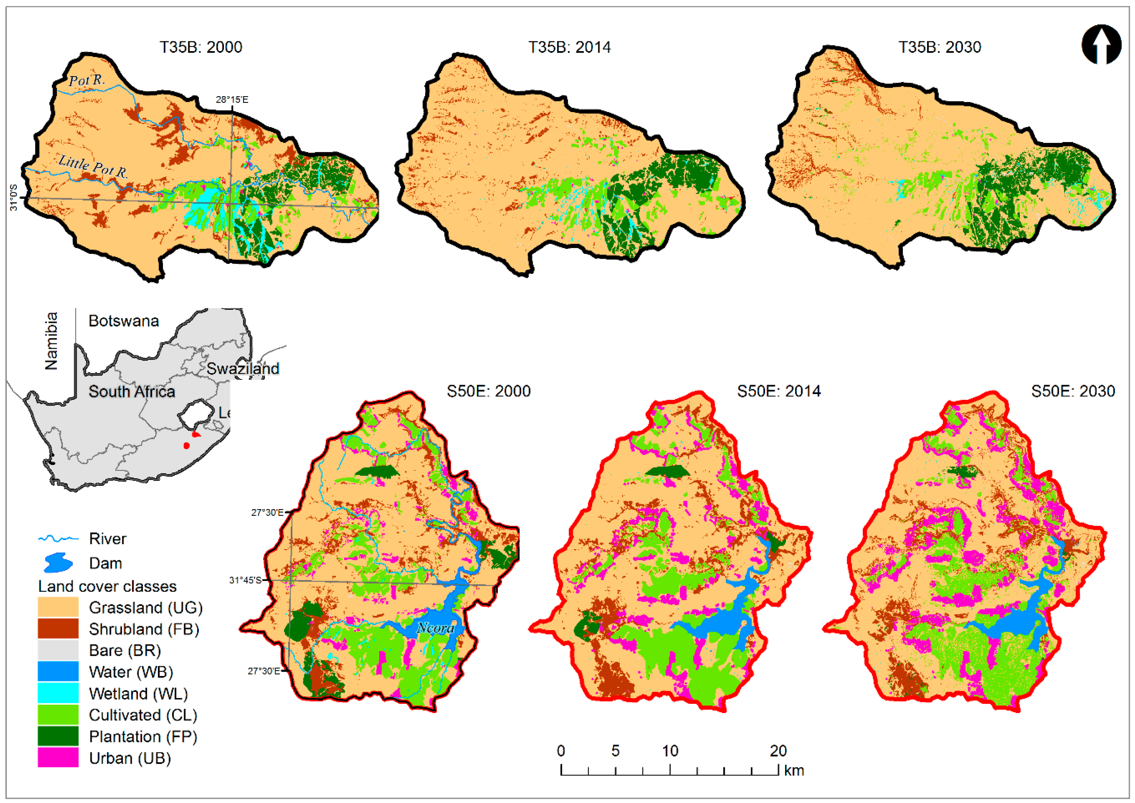
Figure 2.
Processing flow to model albedo relationship with land cover.

Figure 3.
Peak season albedo (pSA) trend (top) and histogram of trend (bottom) measured with MODIS and Landsat for T35B and S50E between 2000–2014.
Figure 3.
Peak season albedo (pSA) trend (top) and histogram of trend (bottom) measured with MODIS and Landsat for T35B and S50E between 2000–2014.
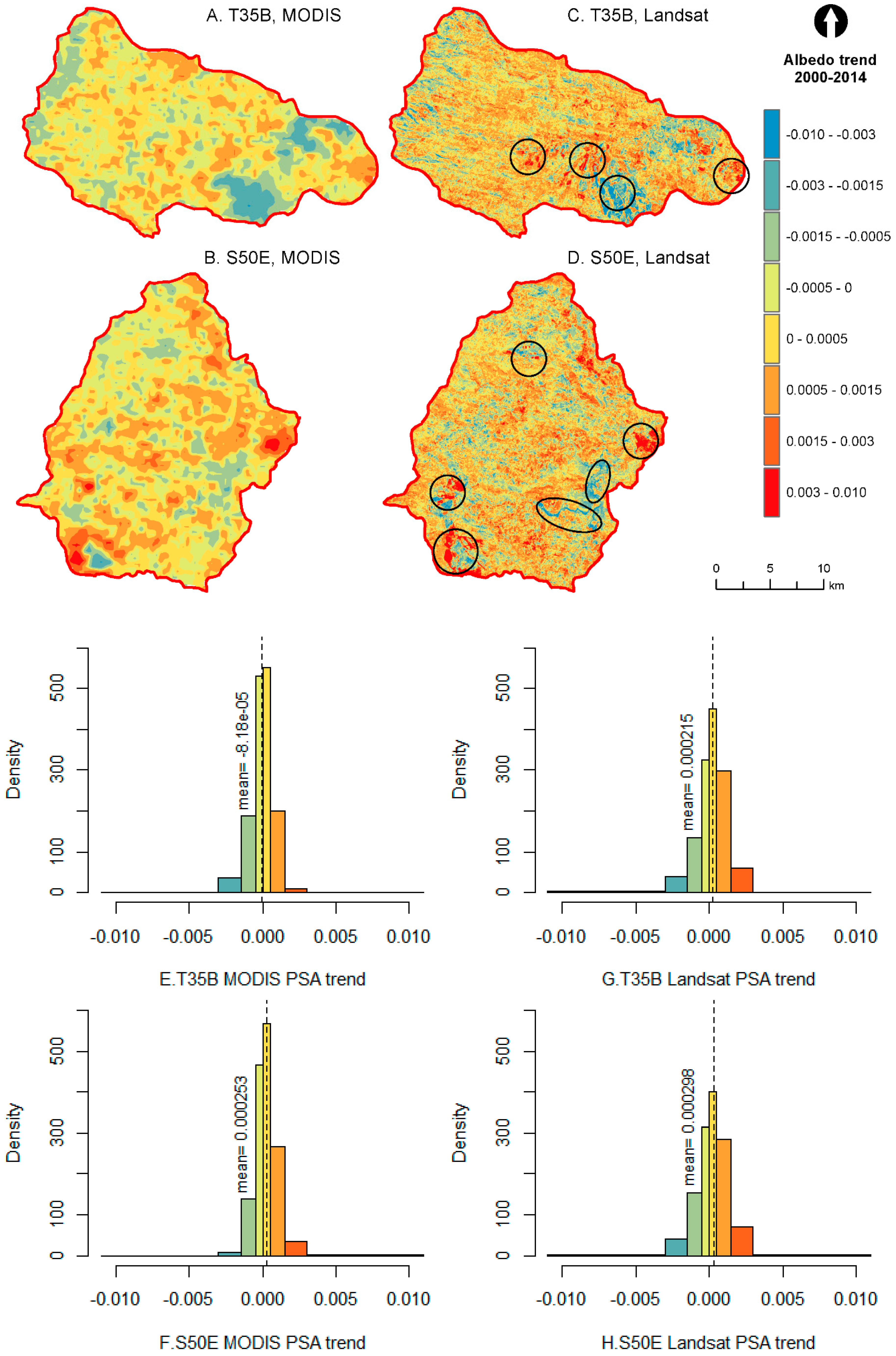
Figure 4.
Mean annual PSA (A,B), net primary production (NPP) (D,E), evapotranspiration (ET) (F, G) and normalised difference vegetation index (NDVI) (H,I) values respectively for T35B (left) and S50E (right), with bar plot of annual rainfall (C). LOcal regression (LOESS) curve in red, linear regression curve in dotted lines.
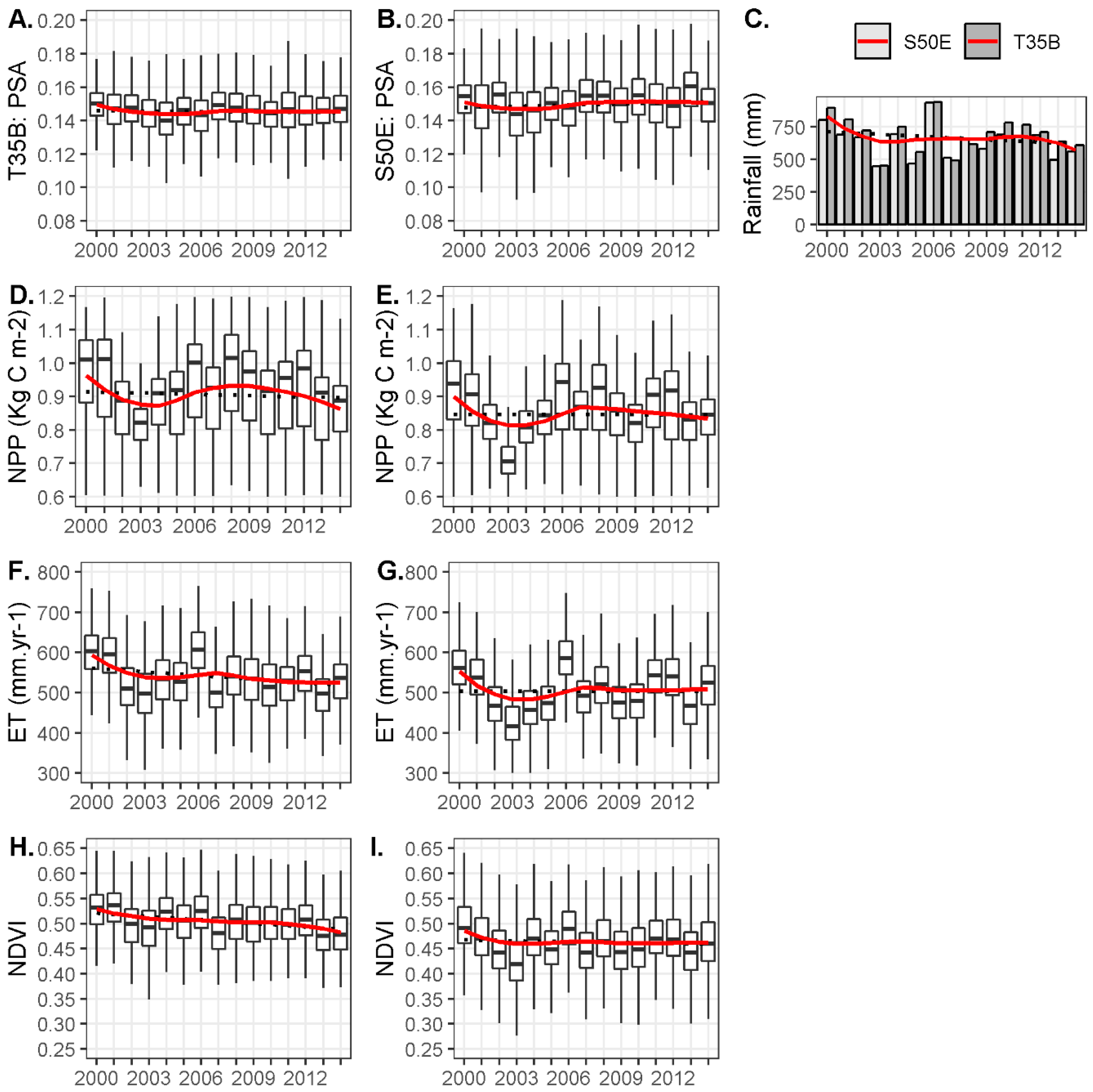
Figure 5.
Spatial distribution of albedo correlation with NPP, NDVI and ET.

Figure 6.
PSA in persistent land cover classes over the study period.
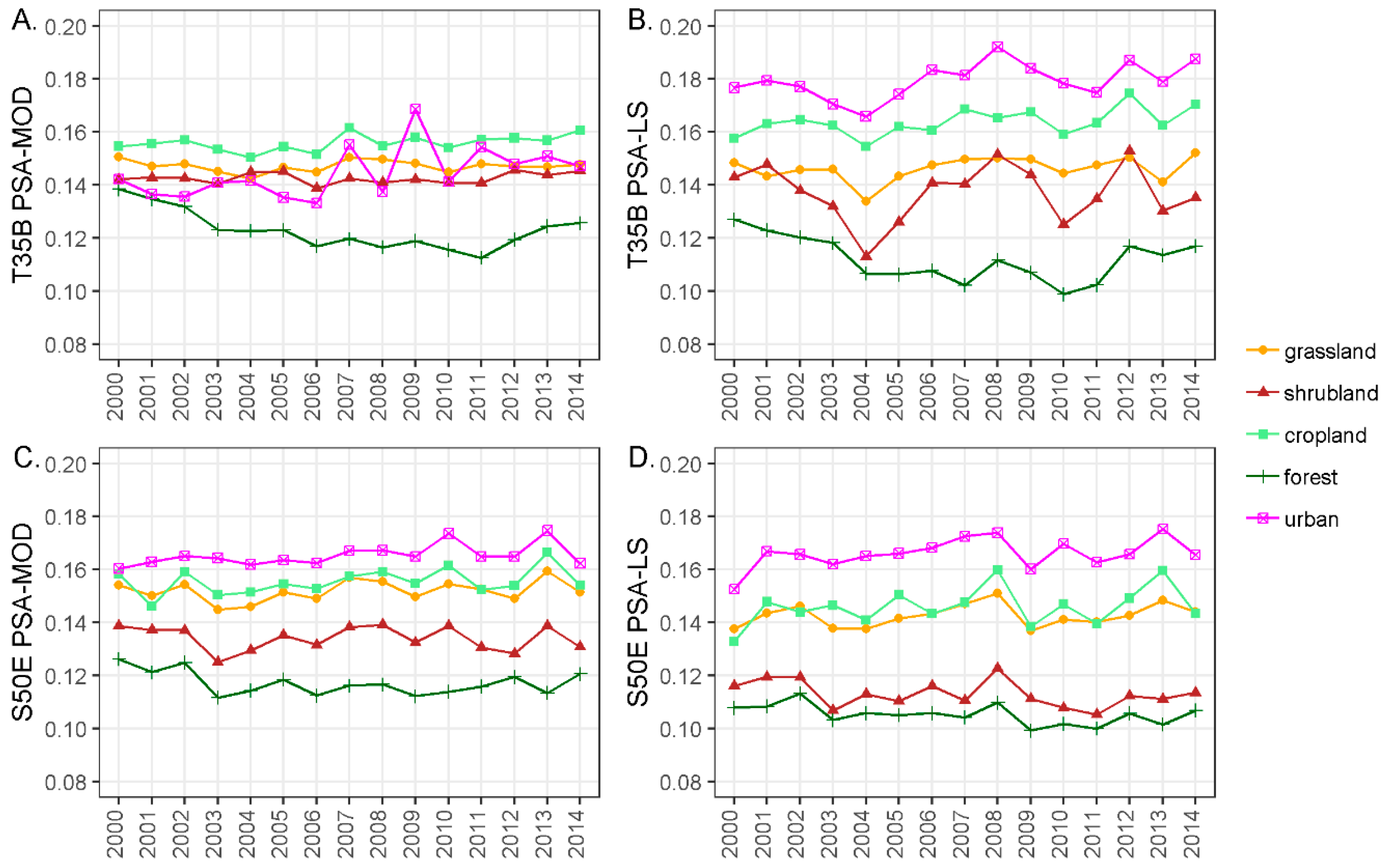
Figure 7.
PSA in transition classes over the study period (If-woody encroachment, Re- reclamation, R-afforestation, CAT-catchment average, Ia-increased cultivation, Iu-increased urban, D-deforestation, De-degradation, A-abandonment).
Figure 7.
PSA in transition classes over the study period (If-woody encroachment, Re- reclamation, R-afforestation, CAT-catchment average, Ia-increased cultivation, Iu-increased urban, D-deforestation, De-degradation, A-abandonment).
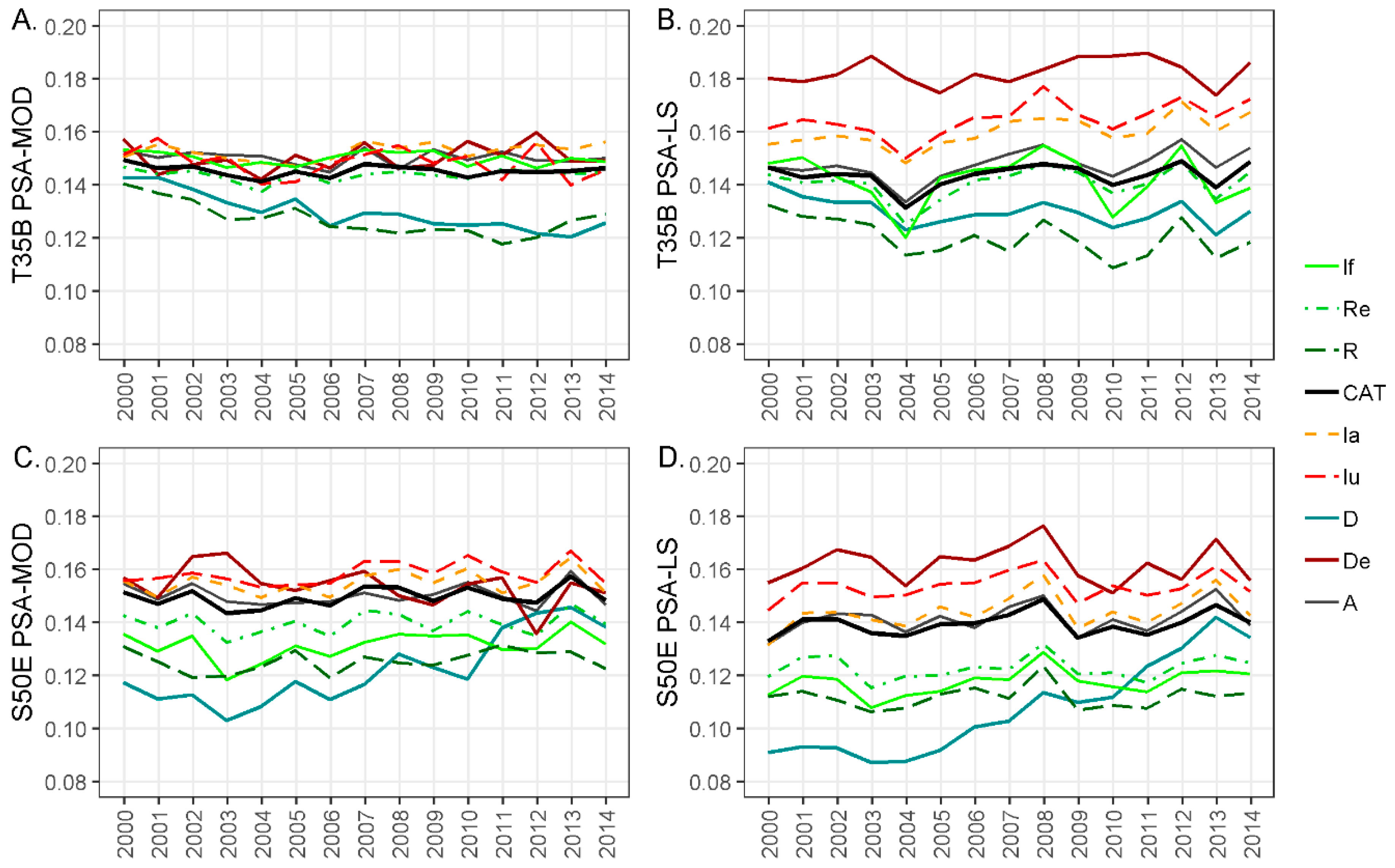
Figure 8.
Estimated trends on three selected points decomposed using season-trend model (STM) in package greenbrown in R. Red squares indicate structural breaks, while blue and green stars indicate significance of trend segments.
Figure 8.
Estimated trends on three selected points decomposed using season-trend model (STM) in package greenbrown in R. Red squares indicate structural breaks, while blue and green stars indicate significance of trend segments.
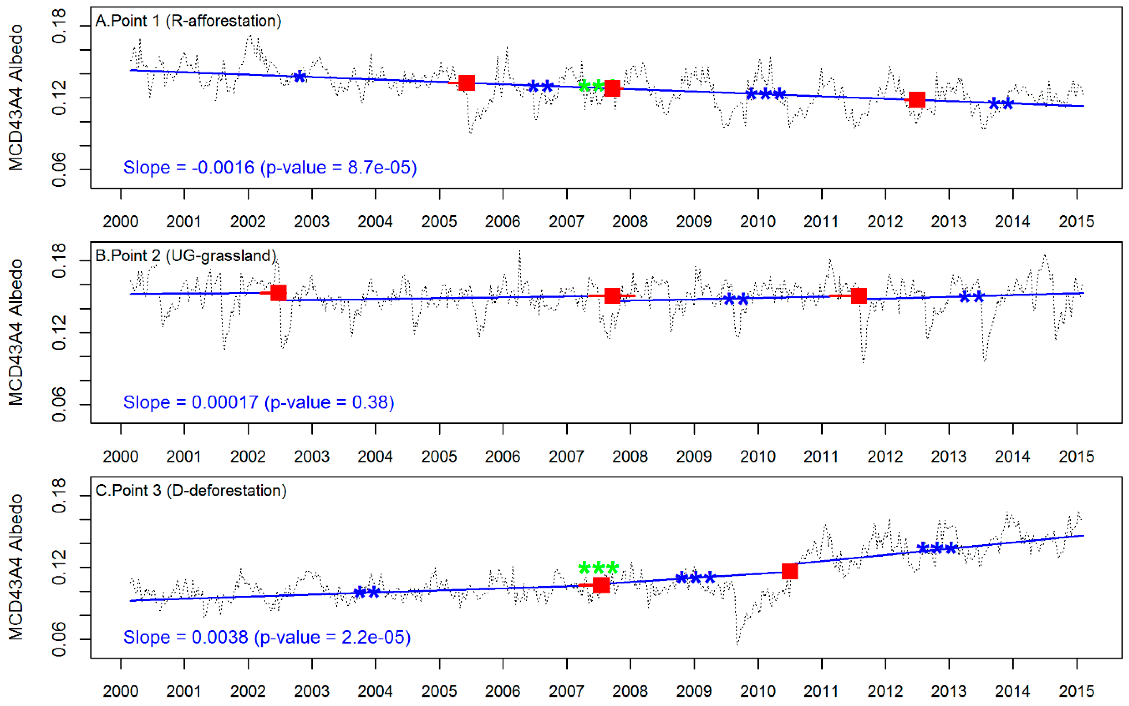
Figure 9.
Inter-annual variability (IAV) standard deviation (sd) (A-T35B, B-S50E) and seasonal range (C-T35B, D-S50E) measured on all pixels from the 8-day MODIS product.
Figure 9.
Inter-annual variability (IAV) standard deviation (sd) (A-T35B, B-S50E) and seasonal range (C-T35B, D-S50E) measured on all pixels from the 8-day MODIS product.
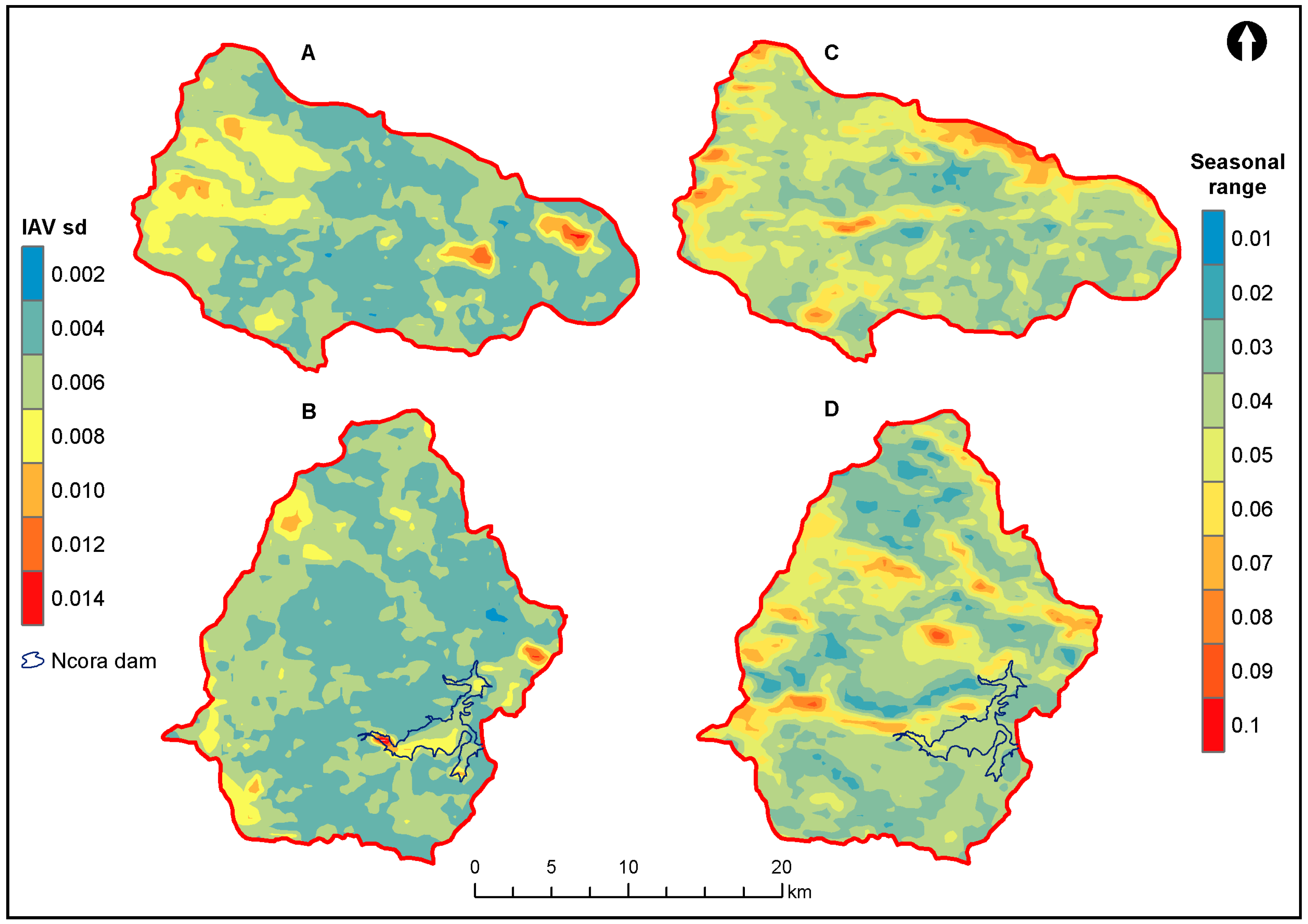

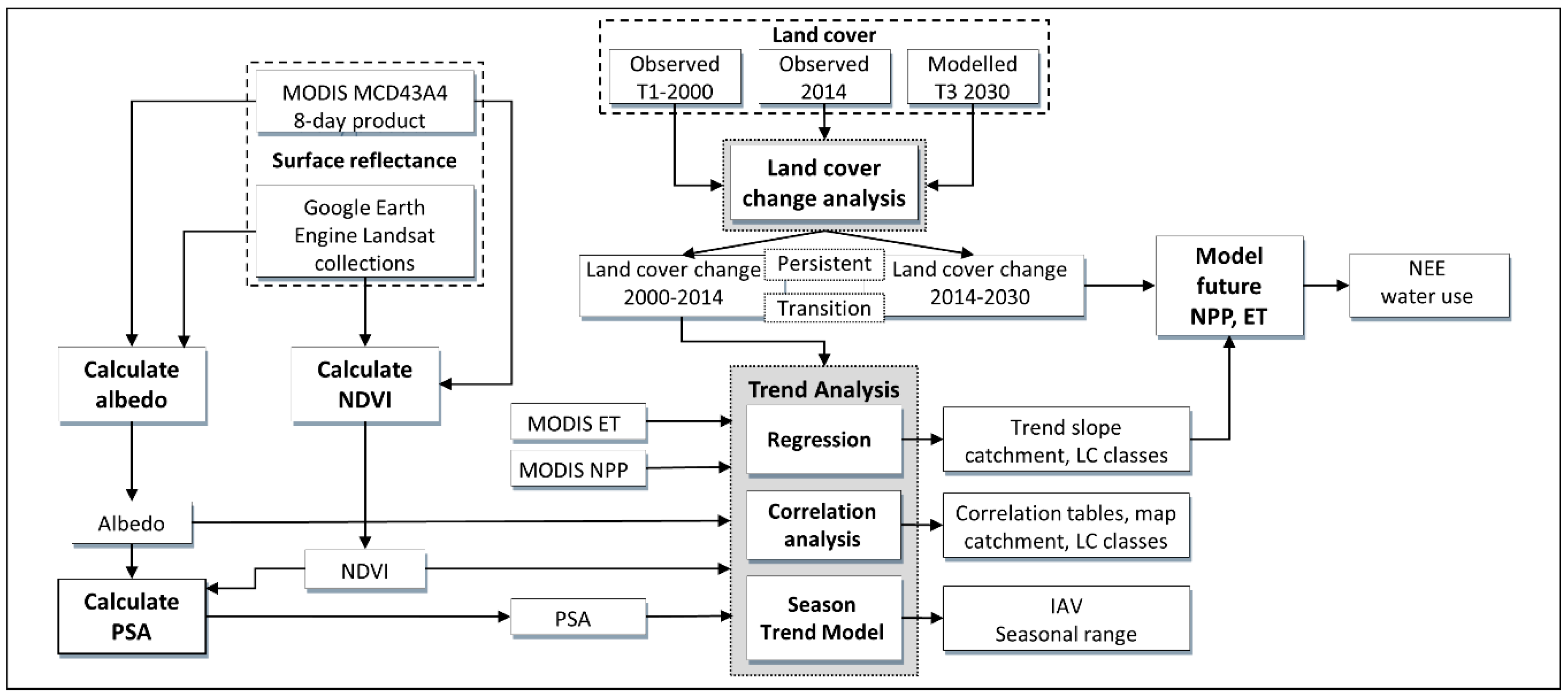
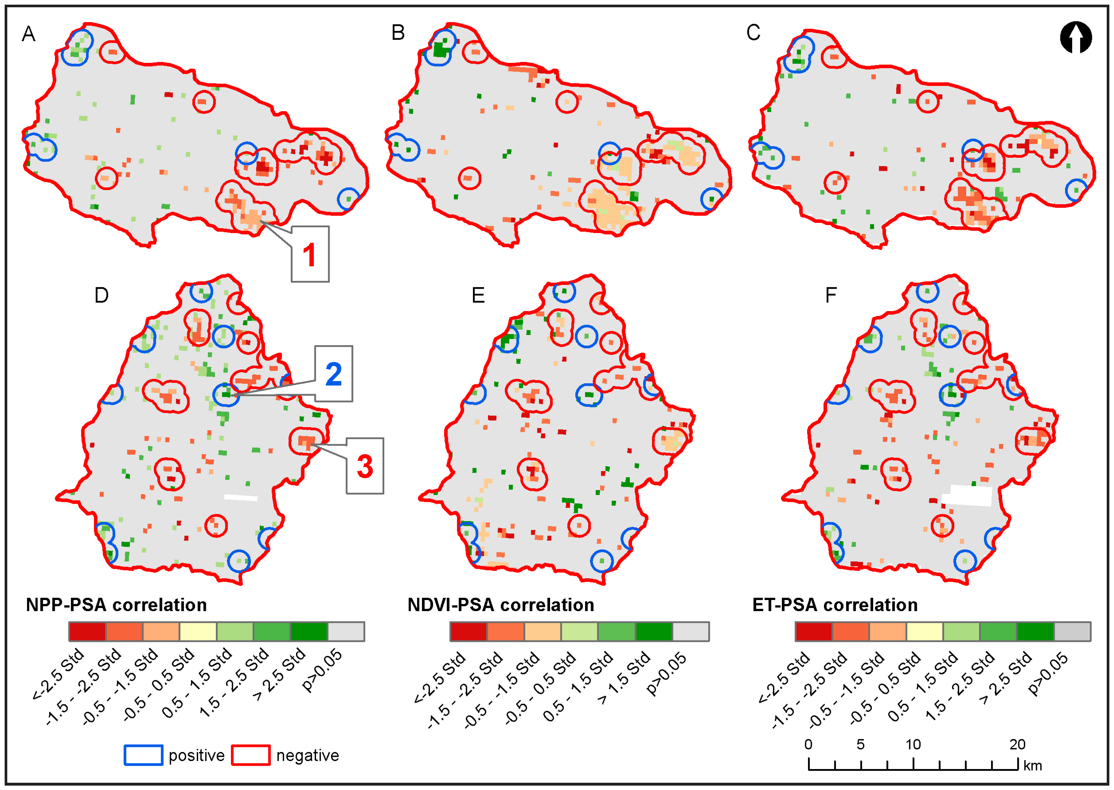
Table 1.
Land cover change trajectories.
| Land Cover Trajectory (Label) | Land Cover Transitions (Expected Albedo Change) | Land Change Category |
|---|---|---|
| Woody encroachment (Ifg) | UG->FB(↓); FP->FB(↑); CL->FB(↓) | Gradual ecological change |
| Abandonment (Ag) | CL->UG(↓); UB->UG(↓) | |
| Degradation (Deg) | UG->BR(↑) | |
| Reclamation (Reg) | FB->UG(↑) | |
| Increased cultivation (Iaa) | UG->CL(↑); FB->CL(↑); WB->CL(↑); WL->CL(↑); UB->CL(↓) | Abrupt change |
| Urban expansion (Iua) | UG->UB(↑); CL->UB(↑); FB->UB(↑) | |
| Afforestation (Ra) | UG->FP(↓); FB->FP(↓) | |
| Deforestation (Da) | FP->UG(↑); FP->BR(↑) | |
| Natural dynamic (Dns ) | UG->WB(↓); UG->WL(↓); WB->UG(↑); WL->UG(↑) | Seasonal change |
UG: grasslands, FB: shrublands, BR: bare, WB: water bodies, WL: wetlands, CL: croplands, FP: forest/plantation, UB: urban.
Table 2.
Constant values used in calculation of albedo from moderate resolution imaging spectroradiometer (MODIS) and Landsat.
Table 2.
Constant values used in calculation of albedo from moderate resolution imaging spectroradiometer (MODIS) and Landsat.
| c0 | c1 | c2 | c3 | c4 | c5 | c7 | |
|---|---|---|---|---|---|---|---|
| Modis | −0.0015 | 0.160 | 0.291 | 0.243 | 0.116 | 0.112 | 0.018 |
| Landsat | −0.0018 | 0.356 | 0 | 0.13 | 0.373 | 0.085 | 0.072 |
Table 3.
Catchment level correlation between PSA, NPP, NDVI and ET.
| T35B | 1 | 2 | 3 | 4 |
|---|---|---|---|---|
| 1. PSA | - | −0.01 | −0.35 | −0.22 |
| 2. NPP | 0.13 | - | 0.51 * | 0.71 * |
| 3. NDVI | −0.28 | 0.31 | - | 0.60 * |
| 4. ET | −0.08 | 0.64 * | 0.57 * | - |
Note. Correlations for S50E (n = 2407) are presented above the diagonal in italics, and correlations for T35B (n = 2162) are presented below the diagonal. * p < 0.05.
Table 4.
Study area albedo values compared to literature.
| S50E | T35B | |||||
|---|---|---|---|---|---|---|
| Land Cover | Landsat | Mean Modis | Landsat | Mean Modis | Literature Value | |
| UG | grasslands | 0.142 | 0.152 | 0.146 | 0.147 | 0.17 [48] |
| FB | shrublands, indigenous as well as invasive trees and bushes | 0.113 | 0.133 | 0.138 | 0.144 | 0.17 [48] |
| BR | bare | 0.163 | - | - | - | 0.20–0.33 [49] |
| WB | water bodies | 0.126 | 0.134 | 0.043 | - | 0.05–0.20 [49] |
| WL | wetlands | 0.120 | - | 0.126 | 0.147 | |
| CL | croplands | 0.146 | 0.155 | 0.163 | 0.154 | 0.163 [36] |
| FP | forest/plantation | 0.105 | 0.117 | 0.113 | 0.124 | 0.11 [48] |
| UB | urban, built-up | 0.166 | 0.163 | 0.177 | 0.157 | |
Table 5.
Total and significant change in land cover classes per catchment, reported in percentage of catchment and change in albedo (highlighted in light grey).
Table 5.
Total and significant change in land cover classes per catchment, reported in percentage of catchment and change in albedo (highlighted in light grey).
| Study | Total Catchment | Significant Change | Negative Sig. Change | Positive Sig. Change | ||||||||||||
|---|---|---|---|---|---|---|---|---|---|---|---|---|---|---|---|---|
| Area | % Area | PSA Change | % Area | PSA Change | % Area | PSA Change | % Area | PSA Change | ||||||||
| LC | MOD | LS | MOD | LS | MOD | LS | MOD | LS | MOD | LS | MOD | LS | MOD | LS | MOD | LS |
| T35B | −0.001 | 0.003 | 11.1 | 11.3 | −0.013 | 0.004 | 7.9 | 4.3 | −0.026 | −0.039 | 3.2 | 7.0 | 0.019 | 0.031 | ||
| P | 82.7 | 81.0 | −0.001 | 0.004 | 7.4 | 8.4 | −0.011 | 0.007 | 5.0 | 2.8 | −0.025 | −0.039 | 2.4 | 5.6 | 0.018 | 0.03 |
| T | 17.6 | 17.8 | −0.004 | 0.001 | 3.4 | 2.8 | −0.017 | −0.002 | 2.7 | 1.4 | −0.027 | −0.04 | 0.7 | 1.4 | 0.023 | 0.036 |
| S50E | 0.004 | 0.004 | 8.5 | 16.1 | 0.016 | 0.017 | 1.9 | 4.1 | −0.018 | −0.026 | 6.6 | 12.0 | 0.026 | 0.032 | ||
| P | 75.4 | 75.5 | 0.004 | 0.004 | 5.4 | 10.9 | 0.013 | 0.013 | 1.3 | 2.9 | −0.023 | −0.027 | 4.1 | 8.0 | 0.025 | 0.027 |
| T | 20.6 | 21.1 | 0.007 | 0.009 | 3.0 | 5.0 | 0.023 | 0.029 | 0.5 | 1.1 | −0.02 | −0.027 | 2.5 | 3.9 | 0.032 | 0.045 |
LC = land cover; MOD = MODIS; LS = Landsat; P = Persistent classes; T = Transition classes.
Table 6.
Modelled net ecosystem carbon exchange (NEE) and water use for persistent land cover classes in S50E (bold) and T35B (italics).
Table 6.
Modelled net ecosystem carbon exchange (NEE) and water use for persistent land cover classes in S50E (bold) and T35B (italics).
| Land Cover Class | UG (Grassland) | FB (Woodyencroachment) | CL (Croplands) | FP (Forest/Plantation) | UB (Urban) | ||||||
|---|---|---|---|---|---|---|---|---|---|---|---|
| Catchment | T35B | S50E | T35B | S50E | T35B | S50E | T35B | S50E | T35B | S50E | |
| % area 2014 | 79.9 | 56.9 | 4 | 10.5 | 6.2 | 18.2 | 8.3 | 1.8 | 0.2 | 9.5 | |
| % area 2030 | 79.7 | 52.1 | 3.1 | 9.9 | 6 | 20 | 9.8 | 0.7 | 0.2 | 14.4 | |
| Net %change | −0.2 | −4.8 | −0.9 | −0.6 | −0.2 | 1.7 | 1.5 | −1.1 | 0 | 4.9 | |
| PSA trend | † | † | * | * | † | †† | *** | ** | ** | †† | |
| %Persistence | 72.7 | 44.7 | 0.4 | 5.5 | 4.3 | 15 | 6.8 | 0.4 | 0.1 | 8.5 | |
| NEE (103 kg C) | 2014 | 2027 | 1633 | 53 | 213 | 138 | 408 | 206 | 71 | 2 | 129 |
| High | 2021 | 1323 | 12 | 181 | 124 | 392 | 238 | 17 | 2 | 236 | |
| Med | 2690 | 1739 | 17 | 237 | 169 | 521 | 292 | 21 | 2 | 316 | |
| Low | 4605 | 2832 | 28 | 383 | 291 | 843 | 358 | 23 | 4 | 518 | |
| ET (103 m3) | 2014 | 1437 | 1182 | 36 | 156 | 96 | 303 | 127 | 37 | 1 | 94 |
| High | 1403 | 855 | 8 | 122 | 85 | 263 | 144 | 10 | 1 | 152 | |
| Med | 1520 | 1007 | 9 | 140 | 93 | 316 | 170 | 12 | 1 | 185 | |
| Low | 1714 | 1163 | 10 | 160 | 105 | 378 | 190 | 14 | 1 | 219 | |
Negative trend *** <−0.0005, ** <−0.0002, * <−0.0000; Positive trend † >0.0000, †† >0.0002, ††† >0.0005.
© 2019 by the authors. Licensee MDPI, Basel, Switzerland. This article is an open access article distributed under the terms and conditions of the Creative Commons Attribution (CC BY) license (http://creativecommons.org/licenses/by/4.0/).
Share and Cite
MDPI and ACS Style
Münch, Z.; Gibson, L.; Palmer, A. Monitoring Effects of Land Cover Change on Biophysical Drivers in Rangelands Using Albedo. Land 2019, 8, 33. https://doi.org/10.3390/land8020033
AMA Style
Münch Z, Gibson L, Palmer A. Monitoring Effects of Land Cover Change on Biophysical Drivers in Rangelands Using Albedo. Land. 2019; 8(2):33. https://doi.org/10.3390/land8020033
Chicago/Turabian StyleMünch, Zahn, Lesley Gibson, and Anthony Palmer. 2019. "Monitoring Effects of Land Cover Change on Biophysical Drivers in Rangelands Using Albedo" Land 8, no. 2: 33. https://doi.org/10.3390/land8020033
Note that from the first issue of 2016, this journal uses article numbers instead of page numbers. See further details here.