Trend Analysis of Las Vegas Land Cover and Temperature Using Remote Sensing


Department of Civil and Environmental Engineering, University of Nevada Las Vegas, Las Vegas, NV 89154, USA
†
Current address: 4505 South Maryland Parkway, MS 4015, Las Vegas, NV 89154, USA.
Land 2018, 7(4), 135; https://doi.org/10.3390/land7040135
Submission received: 30 September 2018
/
Revised: 11 November 2018
/
Accepted: 12 November 2018
/
Published: 14 November 2018
Abstract
:The Las Vegas urban area expanded rapidly during the last two decades. In order to understand the impacts on the environment, it is imperative that the rate and type of urban expansion is determined. Remote sensing is an efficient and effective way to study spatial change in urban areas and Spectral Mixture Analysis (SMA) is a valuable technique to retrieve subpixel landcover information from remote sensing images. In this research, urban growth trends in Las Vegas are studied over the 1990 to 2010 period using images from Landsat 5 Thematic Mapper (TM) and National Agricultural Imagery Program (NAIP). The SMA model of TM pixels is calibrated using high resolution NAIP classified image. The trends of land cover change are related to the land surface temperature trends derived from TM thermal infrared images. The results show that the rate of change of various land covers followed a linear trend in Las Vegas. The largest increase occurred in residential buildings followed by roads and commercial buildings. Some increase in vegetation cover in the form of tree cover and open spaces (grass) is also seen and there is a gradual decrease in barren land and bladed ground. Trend analysis of temperature shows a reduction over the new development areas with increased vegetation cover especially, in the form of golf courses and parks. This research provides a useful insight about the role of vegetation in ameliorating temperature rise in arid urban areas.
1. Introduction
The Las Vegas urban area expanded rapidly during the last two decades [1]. The expansion slowed during 2007–2009 recession, but more recently, the development activities have regained momentum. Las Vegas development has mostly consisted of residential and commercial areas. Being a city in an arid environment with limited water resources [2] and geographically bounded by Federal lands [3], there is a limit to its sustainable urban growth. Thus, it is important to monitor and understand the expansion of the Las Vegas urban area.
Urban expansion is an outcome of the complex interplay of natural and anthropogenic processes linked through feedbacks. In order to understand and model these processes, it is imperative that the rate and type of urban expansion is determined [4]. Urban and social scientists can use this information about the rate and type of urban expansion to develop and calibrate urban sprawl models [5,6]. Moreover, this information can help better understand interaction between natural and urban phenomena and their impacts on issues such as urban temperature, air quality, and flooding [4,7,8]. Furthermore, maps of urban expansion can help urban managers and planners understand the efficacy of previous decisions.
Remote sensing continues to be an efficient and effective way to study spatial change in urban areas [9,10,11,12]. In particular Thematic Mapper (TM) data from Landsat missions has been used to understand urban growth and trends, manage and monitor resources and the environment, and plan future development [13,14,15,16,17]. The spatial resolution of TM data (30-m pixel) can be a limiting factor to capture the details of an urban surface. Therefore, spectral unmixing of surface response using Spectral Mixture Analysis (SMA) is a valuable technique to retrieve subpixel landcover information [15,17,18,19,20]. Nevertheless, the quality of spectral unmixing is highly dependent on the presence and abundance of pure pixels (called endmembers). This difficulty can be overcome by calibrating an SMA model with land cover from high spatial resolution images such as National Agricultural Imagery Program (NAIP) multispectral data (1-m pixel).
This paper presents geospatial aspects of urban growth in Las Vegas using remote sensing and relates the urban land cover change to surface temperature trends. The urban expansion of Las Vegas is studied over the 1990 to 2010 period using TM imagery. A linear spectral mixture model for TM pixel is calibrated using high resolution NAIP classified image to extract subpixel land cover. The trends of land cover classes over the two decades are studied and related to the land surface temperature trends derived from TM thermal infrared images.
This paper is organized as follows. The following subsection is a discussion of relevant literature review. A description of the study area and data used is provided in Section 2. Section 3 describes the remote sensing techniques used for data processing and key results are presented and discussed in Section 4. Section 5 provides a brief summary and description of conclusions.
Background
The spatial nature of urban growth makes it suitable for the application of remote sensing and GIS analysis. Urban areas have complex dynamics and it is imperative to monitor, understand, and predict their growth for sustainable development [21,22]. Due to urban complexity at various scales, remote sensing provides an efficient way to understand urban growth and sprawl [4]. GIS has been successfully applied to model urban sprawl [23,24], determine urban land use change [10], and predict long-term urban growth [25,26]. Donnay et al. [27] has provided a wide range of techniques for urban analysis using remote sensing data including segmentation, temporal prediction, and geostatistical analysis. Bhatta [12] has analyzed various statistical methods in GIS and remote sensing applications to study urban development and growth processes. Wilson et al. [28] has developed a geospatial model to quantify and map urban growth. Land cover change alters the surface energy balance due to anthropogenic materials and urban infrastructure thus, leading to change in surface temperature. Fall et al. [29] analyzed climate data over US and revealed warming trend that could be explained on the basis of land use/land cover change. Wichansky et al. [30] analyzed the New Jersey region and showed through simulation that daytime maximum temperatures over urban landscape are increased more than nighttime minimum temperatures due to enhanced daily temperature range.
Spaceborne remote sensing provides a synoptic view of urban areas and has been applied to many areas of urban studies. Remote sensing has been used to study urban surface runoff [31,32], road networks [33], and impact on surface temperature [2,7,34]. Remote sensing can be applied to characterize urban sprawl [11,35], monitor urban growth [9,13,36], measure land use change [10], and understand surface reflectance from urban areas [37]. Almeida et al. [38] have used Bayesian methods on GIS and remote sensing data to study land use change and generated forecasts of growth trends in Sao Paulo State, Brazil. Abed and Kaysi [39] have used fuzzy logic on GIS and remote sensing data to identify urban boundaries of Beirut area using strong dependency of surrounding areas on the core metropolitan region of Beirut. Bhatta [40] has also modeled urban boundary growth using geoinformatics and shown its benefits to control urban growth and sprawl in Kolkata, India.
Thematic Mapper datasets from multiple Landsat missions have proven very valuable for urban studies [13,15,16]. Landsat TM imagery has been used with spectral unmixing to assess land cover change at multiple scales for the decision making purposes [14]. Landsat TM data has also been used to study urban dynamics [13]. Spectral indices derived from TM imagery such as Normalized Difference Vegetation Index (NDVI) and Normalized Difference Buildup Index (NDBI) have also been useful to analyze urban change [41,42]. Zha et al. [42] have achieved high accuracy urban map of Nanjing city in China using NDBI and NDVI. In particular, NDBI is based on the difference between shortwave infrared and near infrared reflectances to identify buildings and transportation infrastructure. Huang et al. [43] have analyzed 77 cities of the world using TM data and used cluster analysis to understand the compactness of urban areas. As NDBI and NDVI from TM imagery only provide pixel-based distinction at 30-m resolution, further enhancement is required by using subpixel approaches. Several techniques based on spectral unmixing or SMA of TM surface reflectance have been developed to estimate subpixel land cover information [15,16,17,18,19,20,44,45,46]. Typically, SMA techniques use pure pixel spectral response of land cover classes to estimate fractional land cover in mixed pixels.
The classified high resolution imagery can provide land cover information needed to understand spectral responses of larger pixels. The high resolution data is acquired less frequently and thus poses a limitation in itself. Nevertheless, in combination with lower resolution data which has higher temporal resolution, a meaningful method to retrieve subpixel information can be developed.
2. Study Area and Remote Sensing Data
2.1. Las Vegas Urban Sprawl
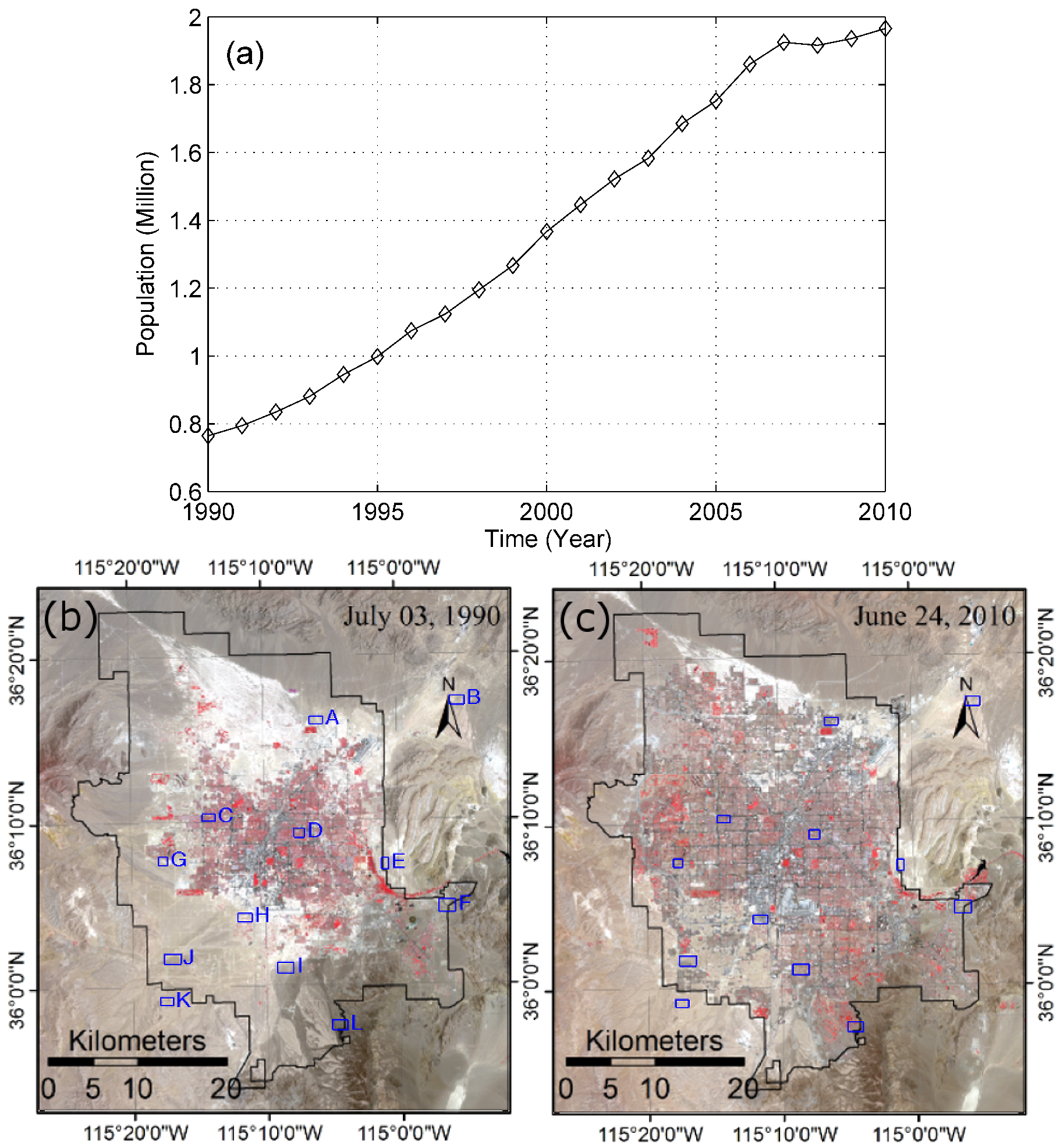
Las Vegas, since its establishment in 1905, has seen spurts of growth stimulated by events such as construction of Hoover dam and the legalization of gambling. In other times, it has continued to attract a population seeking a warm and dry climate, especially senior citizens [1,47,48]. More recently, it was among the fastest growing urban areas. Las Vegas’ population almost doubled during 1990–2010 period accompanied by a rapid urban expansion. Many new residential and commercial developments appeared along with many recreational areas such as golf courses and parks. Figure 1a shows the trend of population increase between 1990 and 2010 [49] and Figure 1b compares corresponding TM false color composite images (i.e., color assignment of red, green, and blue to Bands 4, 3, and 2, respectively), where red shade reflects the vegetation. The two decades considered in this article represent the period of rapid growth of Las Vegas that slowed down due to 2007–2009 recession. This study is a part of urban land cover analysis conducted for Nevada Division of Forestry to understand the role of urban forestry efforts in relation to urban climate during the rapid growth period. Clearly, the doubling of population has resulted in comparable urban expansion. The spatial patterns in TM images illustrate changes in several land cover types such as roads, high density buildings, and open spaces. Figure 1b also depicts 12 sites (A through K) chosen to understand the effect of NDVI on temperature. These sites represent various changed and unchanged land covers between 1990 and 2010 period.
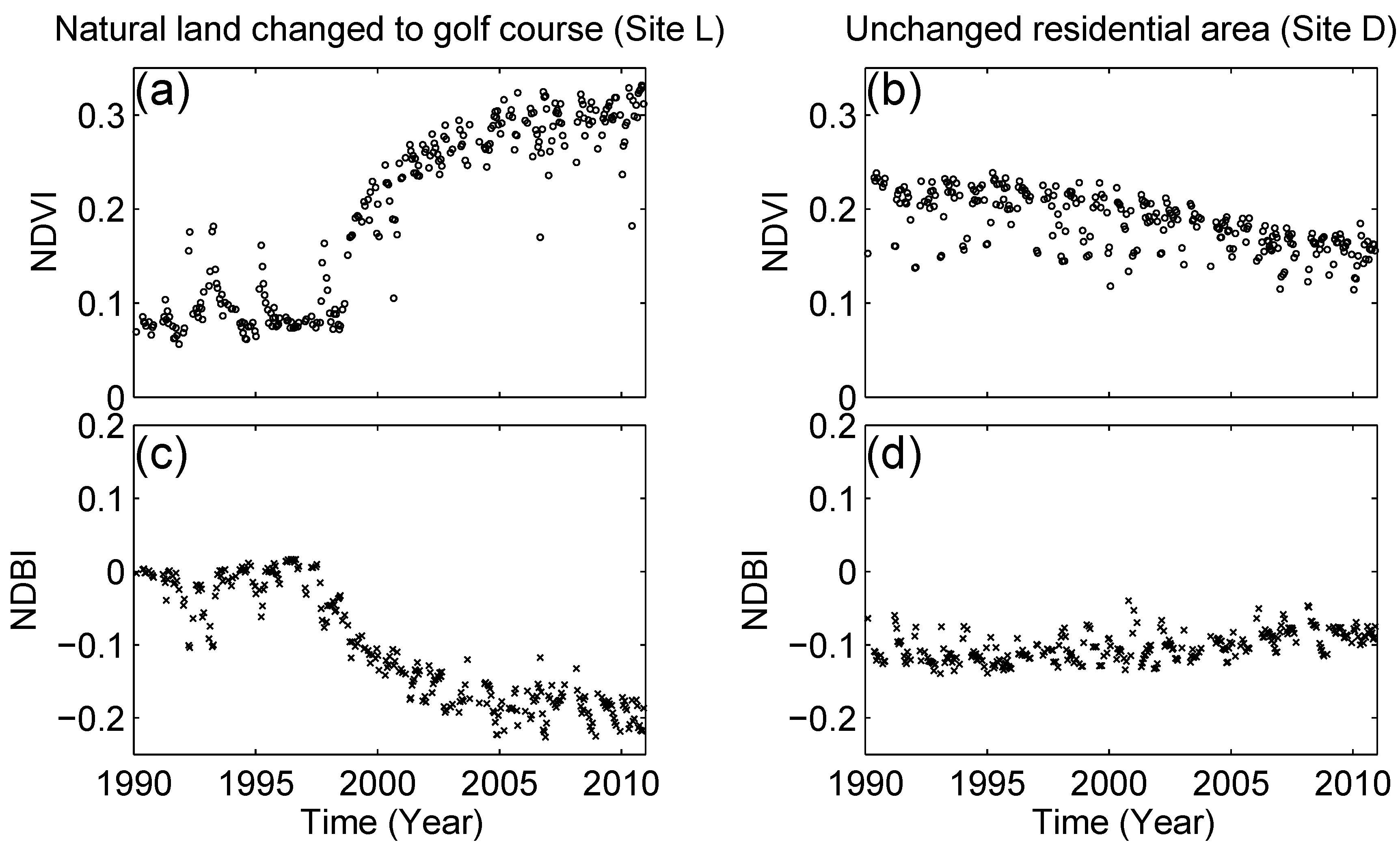
Generally, NDBI and NDVI are used to estimate land cover composition of buildup and vegetated areas. A comparison of NDVI and NDBI derived from TM data is shown in Figure 2 to depict urban development. The left graphs corresponds to a residential site L in Anthem area with a golf course whereas right graphs are over the site D that already existed before 1990. The older development shows very weak trend of NDVI and NDBI. On the other hand, the new development reveals that a gradual change took place during approximately, the 1997–2005 period. Since the water conservation initiatives in Las Vegas did not start until 2003, this new development shows significant rise in the vegetation signature. This visual outlook is not sufficient and a more quantitative understanding of changes in land cover incorporating subpixel information would be useful.
Despite the rapid spatial expansion of Las Vegas, it is approaching an upper limit. Under the Southern Nevada Public Land Management Act of 1998 (SNPLMA), the Bureau of Land Management (BLM) created a disposal boundary around the Las Vegas metropolitan area (solid line bounding urban area in Figure 1b). Any BLM lands within this boundary have been disposed to Clark County. Thus, the disposal boundary defines the limit to the available spatial expansion of the Las Vegas metropolitan area [3].
Land cover changes in Las Vegas due to urbanization impact hydro- and thermodynamics on the surface. Subsequently they impact human life for example in the form of urban flooding and urban heat island effect [50]. Previous work on urban temperature in Las Vegas has shown trends that are related to the urban development [2,34].
2.2. Remote Sensing Data
Landsat 5 Thematic Mapper Data: The Landsat has proven to be a successful mission of NASA and USGS collaboration. The Thematic Mapper onboard Landsat 5 provides a long time series of global multi-band surface reflectance which has found wide applications [51,52]. It is noted that Landsat 5 is the only platform that covers the study period of interest providing data from a single thematic mapper sensor at a resolution useful for urban decadal study. In this research, bands 1–5 and 7 are used for subpixel land cover extraction whereas band 6 is used for land surface temperature estimation. Data conversion procedure as described by Chander et al. [52] and Giannini et al. [53] was followed to estimate surface reflectance and surface temperature. The TM data is available for the whole study period at an average repeat cycle of 16 days and 30-m spatial resolution. In order to ensure meaningful results, the TM imagery was carefully screened and cloudy images were removed. Although Las Vegas has clear sky most of the year, atmospheric correction of images was performed using dark object subtraction method [54].
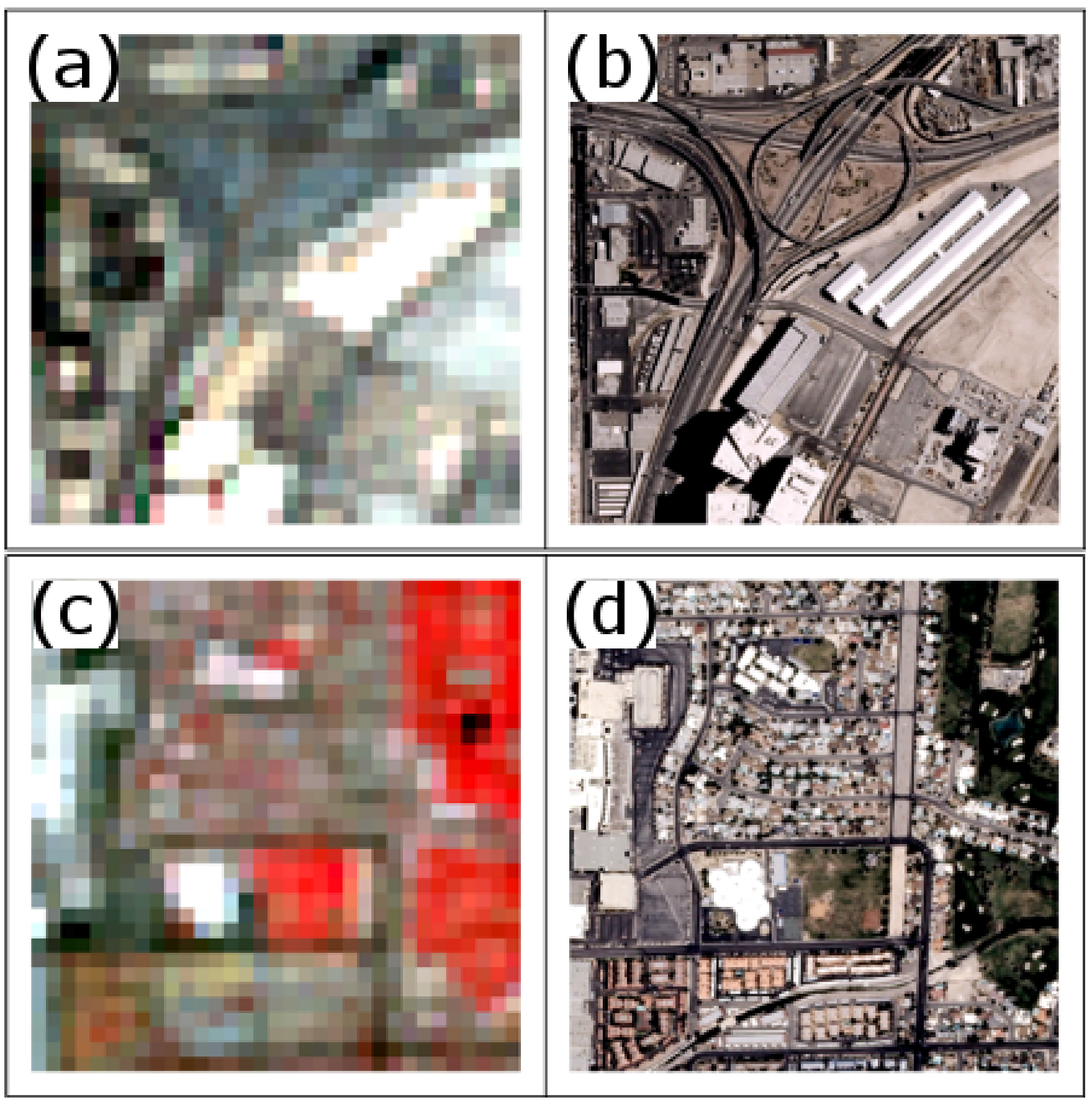
National Agricultural Imagery Program Data: The NAIP was initiated by US Department of Agriculture to map agricultural activities during the growing season. The NAIP imagery is only acquired once or twice a year at 1-m spatial resolution. In general, NAIP imagery is available in 3 bands including blue, green, and red but over some states, 4 band imagery has also been acquired [55]. In this research, the 3-band 2010 NAIP image of Las Vegas valley was used. It was classified into eight classes using supervised image classification. The classified NAIP data provides a detailed view of land surface whereas TM provides a coarse view. Figure 3 compares the NAIP coverage with corresponding 2010 TM image where a TM pixel is 900 m compared to a NAIP pixel of 1 m. Likewise, Table 1 lists and compares the bands of TM and NAIP imagery. The TM imagery closest to the NAIP acquisition time is used for comparison. Being 900 times larger, a TM pixel can be considered as an average response of all the 900 NAIP pixels with combined effect of various land cover classes. The comparative level of detail available in NAIP imagery is evident in Figure 3, where top images show major freeway intersection dominated with asphalt, concrete, and bare soil. The bottom images compare a residential and commercial area showing significant vegetation and roof tiles. When available, these two datasets can be used to decompose spectral response of a TM pixel into its constituent land cover classes.
2.3. Air Temperature Data for Validation
To validate land surface temperature (LST) derived from thermal infrared imagery, ground based dry bulb thermometric data was used that reflects air temperature. These thermometric observations at McCarran Airport (36438″ N 115948″ W) were retrieved from Climate Data Online of National Climatic Data Center of National Oceanic and Atmospheric Administration and used to validate remote sensing-based LST.
3. Method
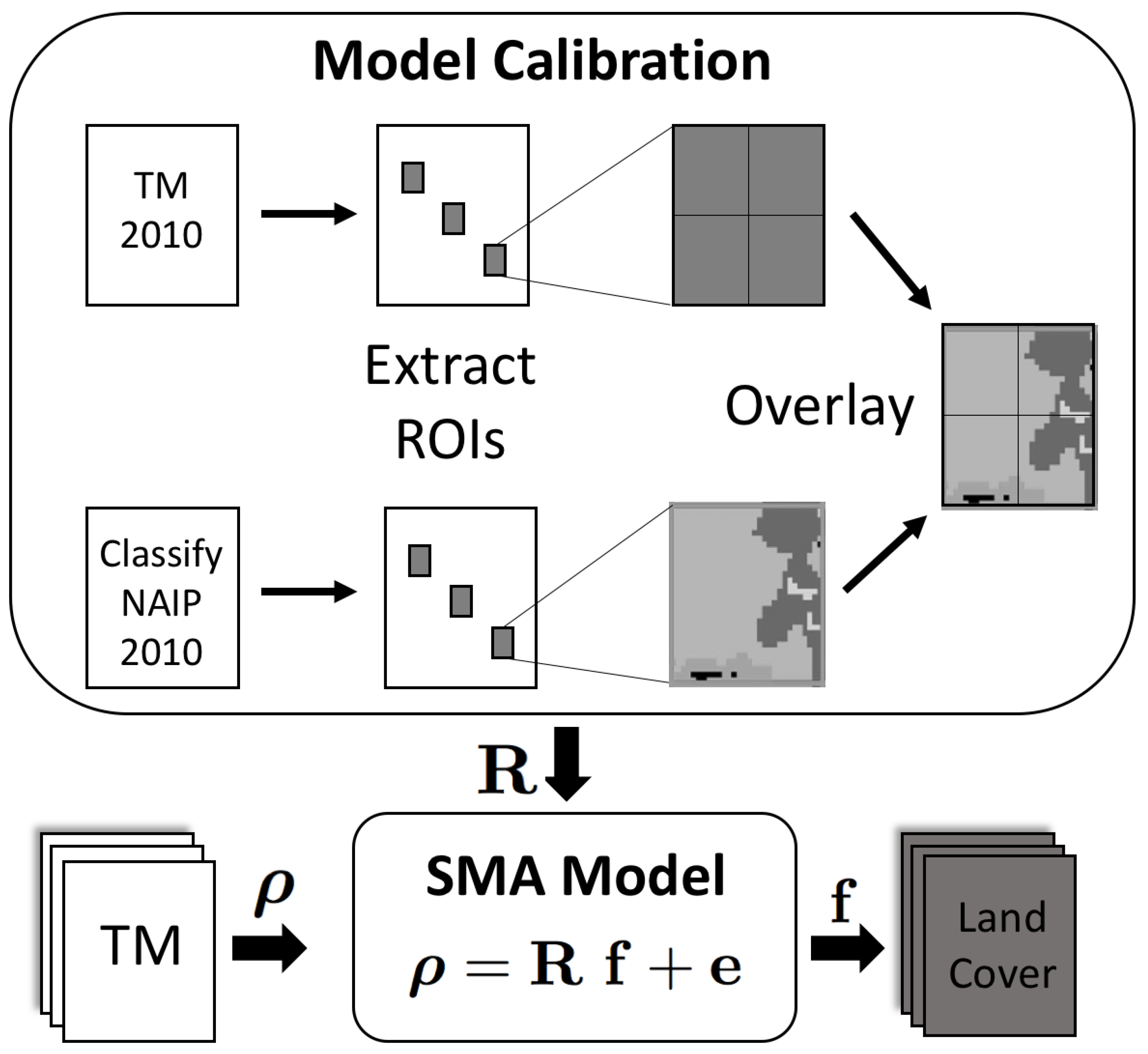
The main approach is to develop a SMA model of a TM pixel in terms of its land cover fractions and to calibrate this model using a NAIP classified image. Then the calibrated model is used to retrieve land cover information from 20 years of TM images. Figure 4 shows the overall workflow of this modeling approach, which is further explained below. Moreover, the corresponding land surface temperature maps are prepared from the TM thermal images.
3.1. NAIP Image Classification
The NAIP imagery is processed with supervised classification where training regions of interest for land cover classes are provided. The Las Vegas urban area is considered to be composed of eight land cover classes including residential buildings (houses), commercial buildings (commercial), asphalt, tree cover, open spaces, water, barren ground (barren land), and bladed ground. These classes represent the general composition of Las Vegas city. The asphalt land cover represents roads and parking lots whereas residential buildings are identified by tiled rooftops. The commercial buildings are differentiated from houses as their rooftops are generally concrete. Vegetation is identified as open spaces and tree cover as these two can be clearly distinguished in the NAIP images and moreover have different spectral responses. Open spaces are primarily parks with grass and residential yard turf. The tree cover is sparse in general with some areas with higher tree coverage including exogenous trees. The barren land represents the undisturbed surface with sparse vegetation (mostly brush) whereas bladed ground represents area that has been prepared for construction. The bladed ground is included to represent the progress of construction activities over time.
Since NAIP image resolution is 1 m, any feature of at least 2-by-2 pixels could be considered as minimum mapping unit. In case of Las Vegas, the minimum mapping units of the chosen classes are variable. Even though features of houses, commercial buildings, open spaces, barren land, and bladed ground were greater than 2-by-2 pixels, any tree cover, asphalt paths, and water ponds smaller than 1-m size could not be detected and classified. In general, it is difficult to achieve good accuracy of classification in high resolution images with fewer bands. In this particular case, lack of near infrared band posed a serious limitation. Nevertheless, a careful selection of training regions representing all eight classes and supervised classification with maximum likelihood classifier was applied achieving a reasonable overall accuracy of more than 80%.
3.2. Subpixel Land Cover Fraction Model
The SMA method is a common approach for retrieving subpixel land cover fractions. This section provides a brief overview of this method to show its connection with the calibration technique. There is a myriad of literature describing and applying SMA to TM data, which can be consulted for more details [15,16,17,18,19,20,44,45,46].
The basis of SMA modeling is that the spectral response of a pixel is a linear combination of the spectral responses of constituent pure land cover classes (endmembers) weighted by the fractional area in the footprint. Mathematically, it is given by
where is the observed surface reflectance of the pixel p in the jth TM band. The summation is performed over N endmembers of choice where is the fractional area of the ith class in the pth pixel. The is a calibration parameter, which represents the surface reflectance of the ith endmember in the jth band. The is the modeling error. Note that j runs from 1 to K where K is the number of bands used in the SMA model. The above equation is conveniently represented in a matrix form as
where is a matrix with elements , is a column vector of the spectral response, is a column vector of the subpixel endmember fractions, and is a column vector of the modeling errors. Each row of corresponds to the spectral response of an endmember. This approach depends on the provision of matrix that is often estimated from training samples of pure pixels representing the endmembers. An image may not have many pure pixels and thus, may not be readily available. Conversely, if the fractional area of the training pixels is available, the above model can be reformulated to estimate . As these fractional areas are available from a high resolution classified image, the model (1) can be rewritten as a system of equations where the are the unknowns. This is the step that is different from conventional SMA approaches. Instead of pure pixels, the model is calibrated using values obtained from a high resolution classified image. In matrix form, the reformulation of (1) is given by
where is a column vector containing P training pixels each having K-band observations, is a matrix, and is column vector. The is a vectorized version of the matrix . is a column vector of the errors. The matrix is created from the training samples of high resolution classified NAIP image whereas the column vector is the corresponding surface reflectance values from the TM bands 1–5 and 7. The classified image results in 900 pixels under each TM pixel as shown in Figure 5. Figure 5 left panel shows a magnified view of the selected NAIP classified pixels and right panel compares an example of training sample of classified image with the corresponding TM data. The land cover fractions under the TM pixels, as retrieved from underlying classified NAIP training samples are used to estimate using the least squares estimation method to get
where is the pseudo-inverse of . The estimated provides as the calibration term for (2). As typically done for SMA approaches, subpixel fractional areas of remaining data can be estimated by solving the following constrained optimization problem for each pixel, i.e., solve
After estimating using the NAIP classified image, Equation (5) is applied to all the cloud free TM images between 1990 and 2010 to prepare their fractional land cover images. These fractional images are used to understand spatial and temporal change of various land cover classes during the study period.
The accuracy of SMA output is highly dependent on the proper selection of the endmembers. The endmembers are land cover classes that are large enough to cover multiple pixels in the image. These are identified by using Pixel Purity Index or by reducing data dimensionality. In the case of dimensional reduction, Principal Component Analysis and Minimum Noise Fraction methods are often used, which limit the number of possible endmembers. In these methods, the number of endmembers cannot exceed the number of dimensions. Moreover, the heterogenous nature of urban surface makes it difficult to find pure pixels in TM imagery. These limitations can be overcome if corresponding high resolution imagery is also available that can be used to calibrate an SMA model.
3.3. Land Surface Temperature Estimation
The land surface temperature () is retrieved from the thermal infrared data (TM band 6). The digital numbers are converted to at-sensor brightness temperature using Chander et al. [52], Giannini et al. [53].
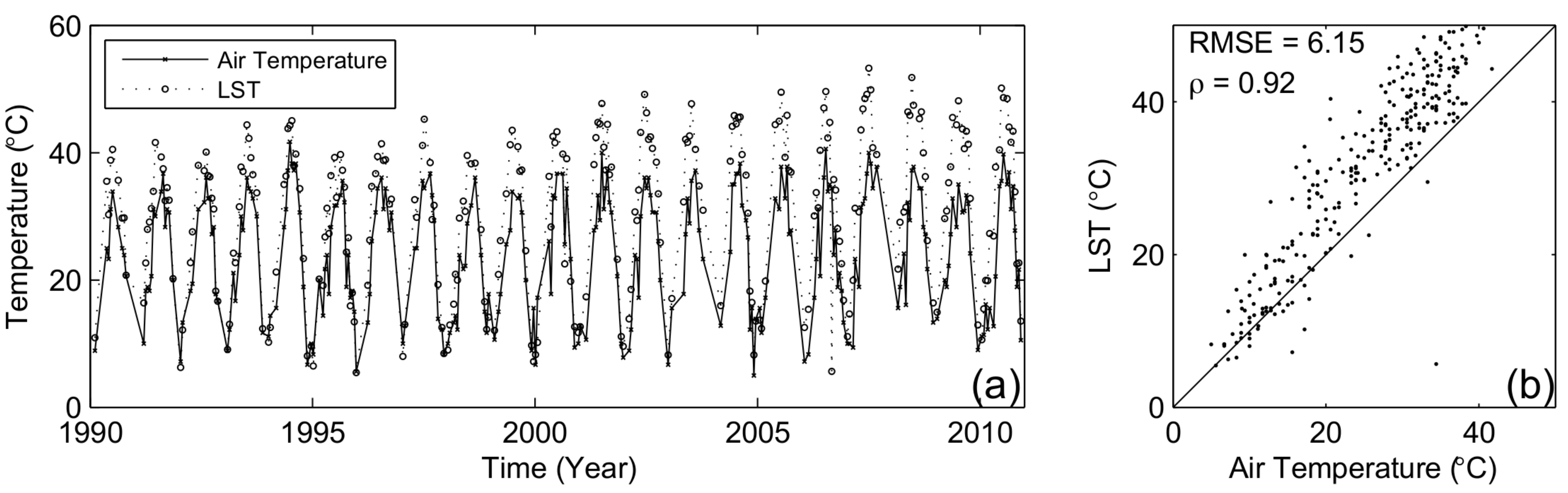
where is at-sensor brightness temperature computed from thermal band radiance () using constants and , is the central thermal band wavelength (11.45 m), is constant ( mK) from Planck’s constant, speed of light, and Boltzmann constant, and is the NDVI-based surface emissivity computed from TM bands 3 (red) and 4 (near infrared). The algorithm is described in detail in [53]. The derived LST is validated using ground-based air temperature data and shown in Figure 6. The time series comparison in this figure reveals that LST matches reasonably with air temperature until 1995 but later reveals higher summer time values. It is noted that the area around the observation point saw additional development of McCarran airport after 1995, a possible reason of change in local thermodynamics. Nevertheless, the winter values match better as also evident in the scatter plot. The overall correlation value between LST and air temperature is 0.92 with RMS error 6.15 C.
4. Results and Discussion
4.1. Subpixel Land Cover Fractions
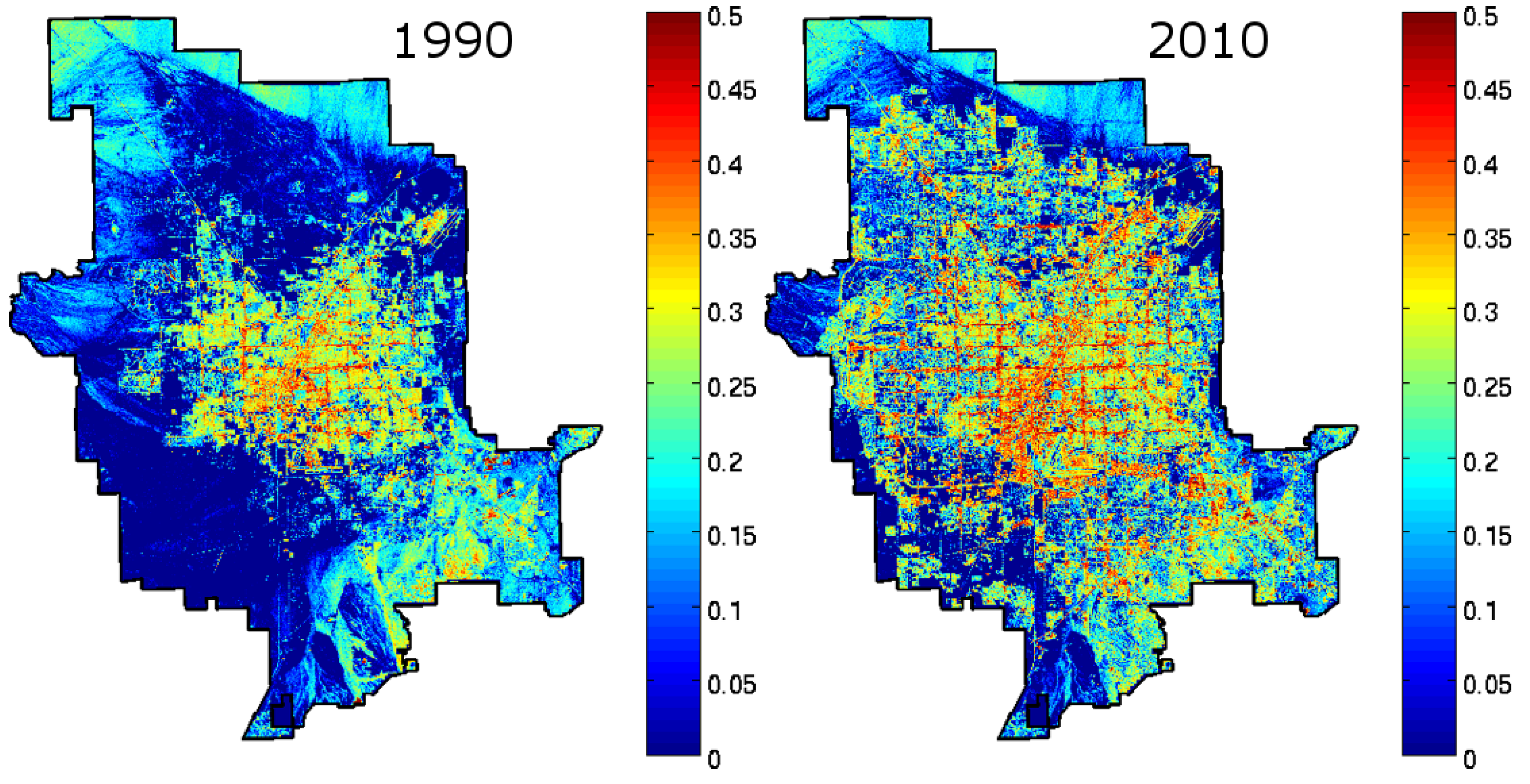
The spatial analysis of the land cover images depicts a consistent behavior about the urban expansion in Las Vegas. For example, Figure 7 compares the maps of land cover fraction of asphalt between 1990 and 2010. In these maps, the high values of asphalt fraction shown as red correspond to the roads and parking lots. The analysis showed that the area covered by asphalt increased from ≈150 km in 1990 to ≈250 km in 2010. As new road infrastructure appears on the landscape, it promotes further urban development and subsequently further extension and enrichment of road network. The extension implies lengthening of roads beyond the existing urban limit and enrichment implies increasing road linkages within the existing urban area. In Las Vegas valley, the road network expansion is a surrogate of the urban expansion and shows that it is reaching its limit of the BLM disposal boundary. In a similar comparison of the houses class, land cover area showed a much greater fractional increase than the asphalt whereas the commercial class showed a relatively lesser increase.
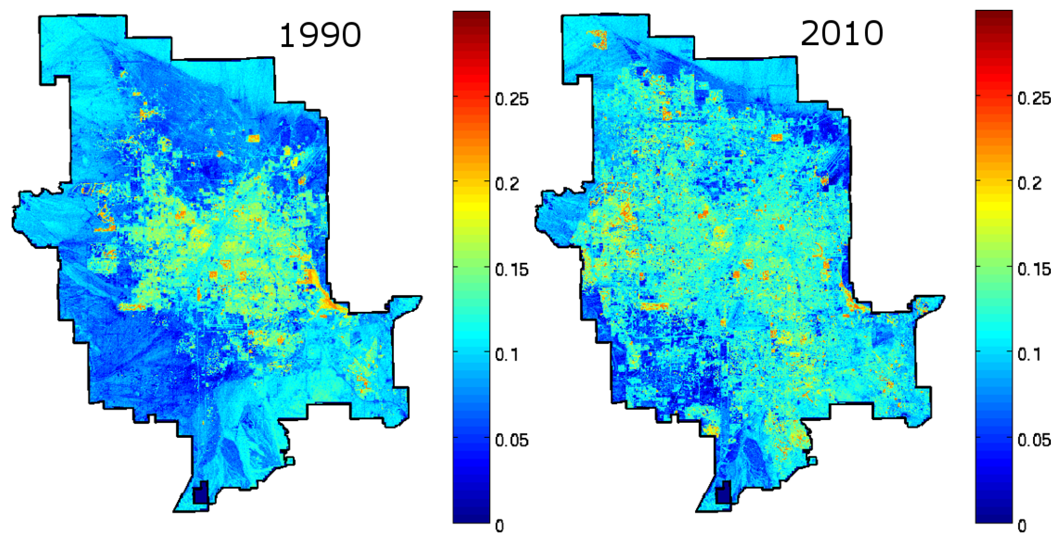
The land cover fraction of tree cover, open spaces, and water have negligible change over the study period. For example, Figure 8 compares the tree cover fraction change over the two decades. The total area of the tree canopy increased from ≈120 km in 1990 to ≈130 km in 2010 (depicted as shades of green and red). Although this increase is small but it is spatially distributed over the whole urban area. Similar to the road network, the tree canopy expansion in Las Vegas is a direct measure of the urban growth and reveals that the Las Vegas expansion is reaching its spatial limits. In Las Vegas, the expansion of the tree canopy class also reflects an increased water demand. Although the best practices of urban forestry guide that the indigenous desert plants are grown, there is some provision of water through a drip irrigation system. In 2003, Las Vegas also promoted xeriscaping practices to conserve outdoor water use. The analysis presented in this paper did not reveal any significant impact of xeriscaping. The impact is expected to reveal in the land cover fractional area of open spaces which showed negligible change.
The land cover fraction of the barren land and bladed ground showed reduction in the area. The barren area is expected to reduce as it is being converted into other urban land surfaces. The reduction in the bladed ground reflects that the construction activity reduced in the year 2010. In order to understand the trends during the 20-year period, a time series analysis of the land cover fractions is presented next.
4.2. Trend Analysis of Land Cover Fractions and Temperature
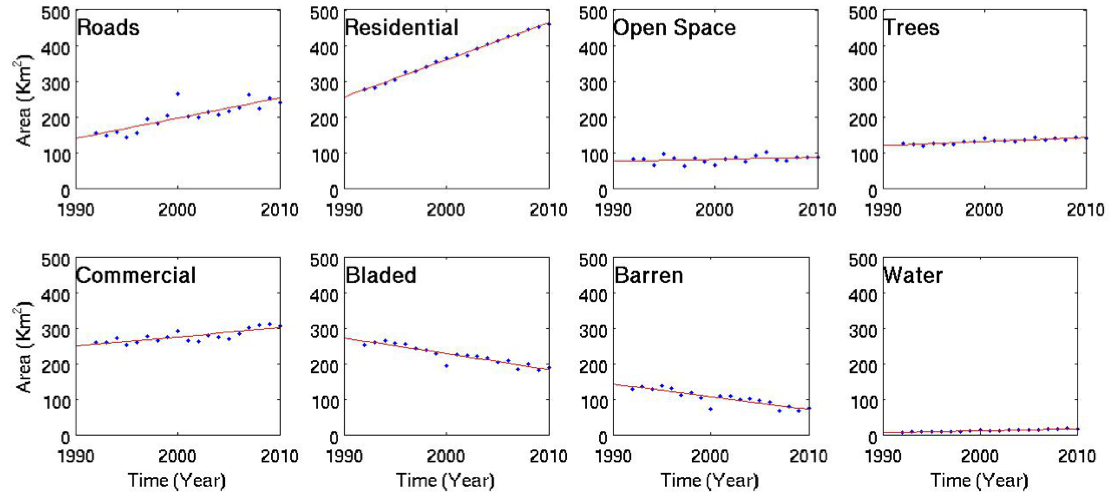
This section discusses temporal variation in the land cover fractions over the study period and explores its relation to the temperature change. Figure 9 shows the time series plots of the surface area (km) of each land cover and the regression line through the data points. The urban growth in Las Vegas followed an overall linear trend. The variability about the trend can be attributed to the inherent fluctuations in the remote sensing imagery due to the solar illumination angle and seasonal variations. Nevertheless, the behavior of trend lines of various land cover classes are consistent with each other. As found through the spatial analysis, temporal variations reveal a consistent result where the houses, asphalt, and commercial classes have gradually increased whereas the barren land and bladed ground have gradually decreased. The tree cover, open spaces, and water, show minute increasing trends.
The slope of the trend lines is the rate of change of the surface area of a given class per year. Table 2 lists the rate of change of each land cover and reveals that a maximum occurred for the houses (10.5 km/year). It is followed by the asphalt (5.7 km/year) and the commercial (2.6 km/year) classes. These three classes reflect the key compositions of an urban growth. The tree cover, open spaces (grass) and water show negligible increase. Note that the open spaces represent yards and public parks, whereas water class is primarily residential pools and ponds in public parks. The classes of barren land and bladed ground decreased at a rate of 3.6 and 4.5 km/year, respectively. The bladed ground area trend was expected to mimic the variation in construction activity in Las Vegas. It may be correlated to the barren land class due to their similar spectral signatures. Nevertheless, this result can be interpreted as an overall reduction in the natural landscape which is replaced by the urban land cover classes.
The land cover trends derived from remote sensing data reveal that the urban spatial expansion of Las Vegas has followed a linear trend. This is insightful as urban growth is often commonly thought to be exponential. Moreover, the Las Vegas urban area has experienced most expansion in the residential sector followed by the asphalt which reflects increased transportation infrastructure. Often urban development is believed to lead to the urban heat island effect as urban growth increases retention of heat in the high specific heat urban materials (asphalt and concrete). Previous studies have shown that the trends of temperature in arid regions behave contrary to this belief [34,56]. In arid regions, the temperature has been observed to reduce after construction of a new development. This is attributed to the change of a barren surface to vegetated surface with more water and consumptive use.
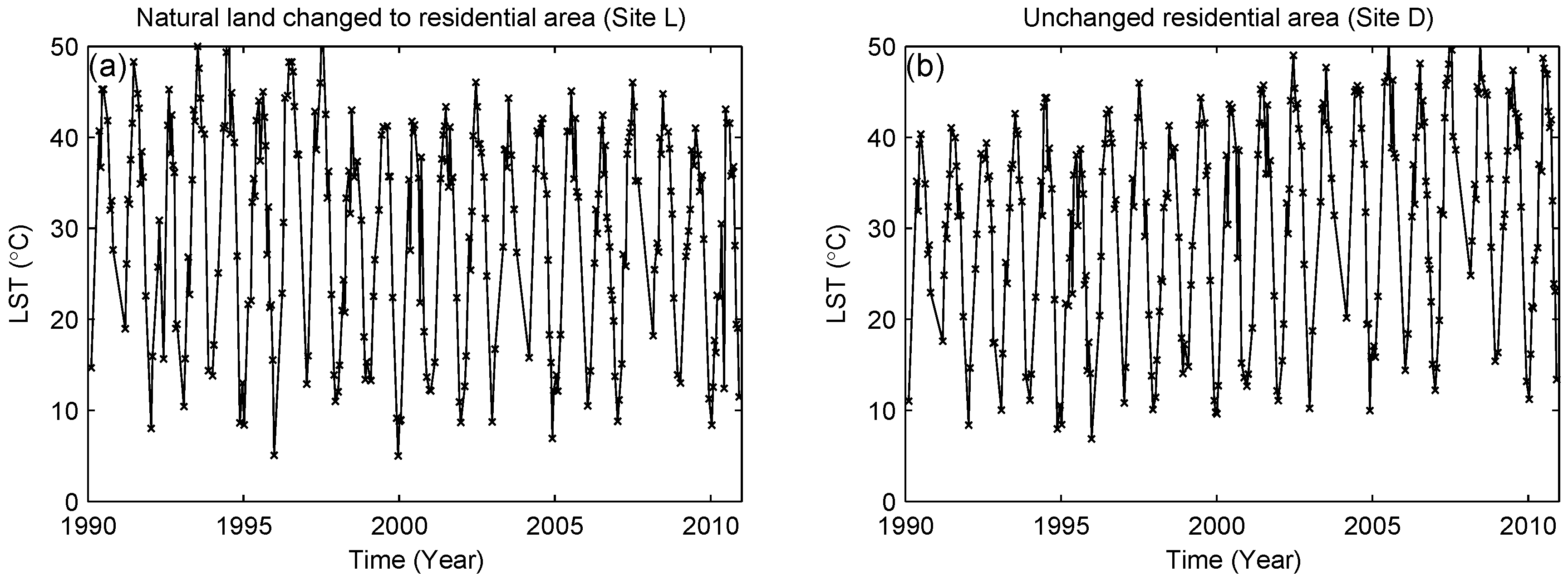
Figure 10 shows a time series plot of the land surface temperature at a sites L (a) and D (b). Comparing with the corresponding NDVI and NDBI plots of these sites (shown in Figure 2) reveals that site L temperature decreased after 1997 whereas NDVI increased. On the other hand, site D underwent a gradual increase in temperature matched by a gradual decrease in NDVI. Such trends are observed in various parts of Las Vegas showing opposing trends of LST and NDVI. An increase in the vegetation at these points is also revealed by ancillary observations from Google Earth high resolution imagery when available. Such inverse relationships between LST and NDVI are also observed by Yue et al. [57] over various land covers in Shanghai, China. In Las Vegas, this relation is consistent with the increasing trends of tree cover, open spaces, and water revealed in Figure 9. Even though the increase in vegetation is small, it shows impact in reducing the temperature. The contributing factors could include shadow on surface and role of vegetation in redirecting heat through transpiration.
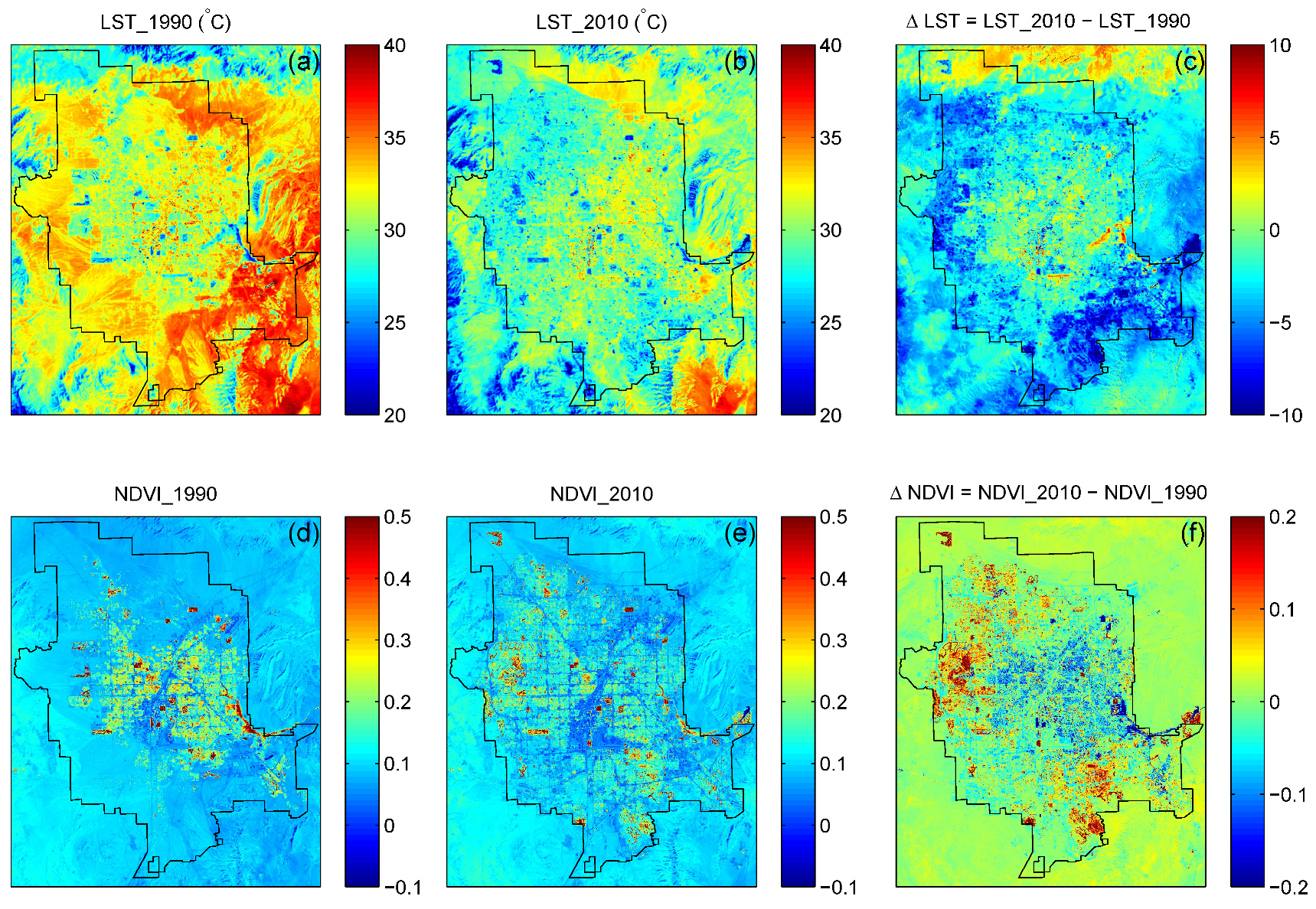
To further confirm, this behavior, Figure 11 illustrates change in LST and NDVI between 1990 and 2010. These images are computed using annual averages of LST and NDVI during 1990 and 2010, respectively. The two-decadal change is shown as the difference image. A comparison of LST images shows relatively lower temperature in 2010, especially in the areas that were developed after 1990. These areas can be verified in the NDVI images showing urban expansion. The highest rise in NDVI is observed in the new developments with golf courses and parks. Similar to the previous observation, pixels showing increased NDVI correspond to pixels with decreased LST.
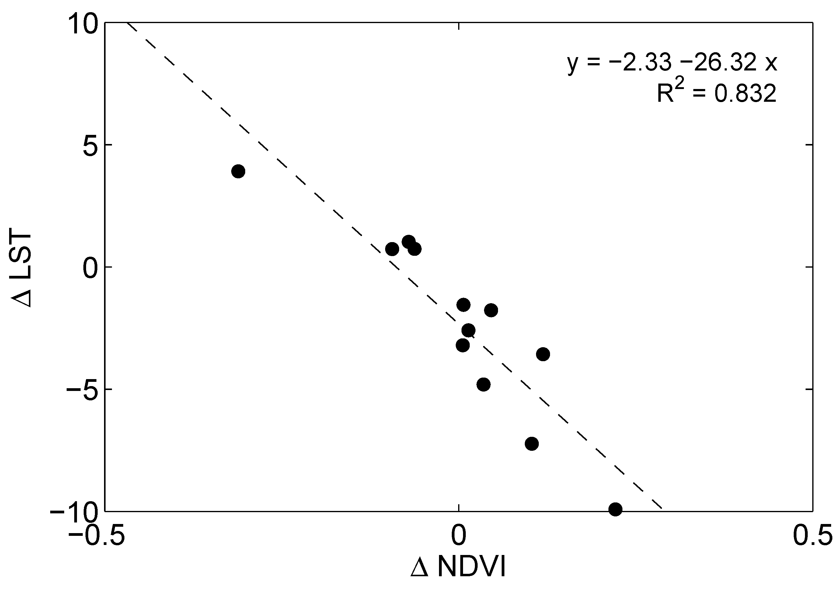
To quantify this effect, the averages of LST and NDVI over the sites A through L are computed for 1990 and 2010 and listed in Table 3. The differences are listed in columns titled LST and NDVI. Additionally, the land cover for the two years is provided to analyze the effect of land cover change. Five sites represent areas with no land cover change (A, B, C, D, and K) whereas six sites represent areas where rural land cover was changed to some form of urban land cover (F, G, H, I, J, and L) such as residential, commercial, and open space (golf course and park). One site (E) also is chosen where land cover changed from a park to residential land cover. The differences reveal that sites where rural land cover was changed to residential, park, and golf course land cover, LST is negative (decreased) and NDVI is positive (increased). Overall, LST and NDVI have opposite signs. This is further elaborated in Figure 12 as a scatter plot between LST and NDVI. A regression line is fitted with and establishes a strong relation between LST and NDVI over the selected sites. Similar phenomena have been observed in many arid cities around the world and often referred as urban cool island effect [58,59,60].
The analysis of the land cover change and the corresponding relation between LST and NDVI shows that the Las Vegas growth has lowered LST in areas where NDVI increased. The expansion in residential areas has brought about significant increase in roads but also increased vegetated cover in some area as trees, golf courses, and parks. This has resulted in an interesting behavior of the temperature trend which reveals that the vegetated cover has counteracted the impact of temperature rise due to the urbanization.
5. Summary
The urban expansion of Las Vegas was studied using remote sensing data. Las Vegas grew rapidly during 1990–2010 period due to accelerated building of residential neighborhoods to accommodate people moving for better wages and warmer climate. Remote sensing is a useful way to study the response of landscape and environment to such rapid urbanization. In particular, the response of land surface temperature can be analyzed that is directly related to urban geophysical processes including hydrology and aerodynamics impacting the quality of urban living.
This research used remote sensing techniques to quantify land cover change in Las Vegas and analyzed its surface temperature change. Spectral mixture analysis is used to retrieve subpixel land cover fraction of eight classes. Generally, SMA models are applied using endmember spectral information. This research demonstrates a calibration technique for SMA modeling that takes advantage of high resolution classified NAIP image. It is shown that when pure pixels are difficult to identify or insufficient, a high resolution classified image can be used to calibrate the SMA model. This approach provides the spectral response of pure land cover classes through the known fractional areas derived from a high resolution image.
The results from inversion of SMA model reveal that the rate of change of various land cover classes followed a linear trend in Las Vegas. The largest increase occurred for the houses class followed by roads and commercial areas. The largest expansion has been due to houses and providing roadway access to them. Being a city in an arid region, this expansion has been accompanied with increase in vegetation cover in the form of tree cover and open spaces (golf courses and parks). Since, the pre-development surface was primarily desert landscape with brush, various post-development localities with more vegetation have increased shading, water consumption, and evapotranspiration. Among other land cover classes, the increase in water class is also observed most likely due to residential pools and ponds in public parks. The results reveal a gradual decrease in the barren land and bladed ground class, which is consistent with the relevant increase in the other land covers.
The trend analysis of the LST revealed an inverse relation with NDVI, especially in the new developments of Las Vegas. This result is consistent with the previously reported findings of temperature change in arid regions [34,56,59,61]. Moreover, despite an increase in the heat absorbing asphalt and concrete, even an increase in vegetation cover can play a key role in counteracting the impact of temperature rise. The overall cooling response is observed in vegetated new developments due to shading from vegetation as well as increased water use. It is noted that there are many other inter-related factors related to surface geometry and materials that must be considered for a complete thermodynamic analysis of urban surface. Nevertheless, this research provides a simple relation between LST and NDVI with useful insight about the role of vegetation in ameliorating temperature rise in an arid urban areas.
Funding
The funding for this work was provided by Nevada Division of Forestry through a subaward of grant from US Forest Service, US Department of Agriculture (Award # 09-DG-11046000-607). The author is thankful to Adam Black for helping in the temperature trend analysis.
Conflicts of Interest
The author declares no conflicts of interest.
References
- Acevedo, W.; Gaydos, L.; Tilley, J.; Mladinich, C.; Buchanan, J.; Blauer, S.; Kruger, K.; Schubert, J. Urban Land Use Change in the Las Vegas Valley. 2013. Available online: http://geochange.er.usgs.gov/sw/changes/anthropogenic/population/las_vegas/ (accessed on 15 April 2016).
- Stephen, H.; Black, A.; Ahmad, S. Relating Temperature Trends to Urban Change and NDVI in Las Vegas. In World Environmental and Water Resources Congress 2014@ Water Without Borders; ASCE: Reston, VA, USA, 2014; pp. 866–875. [Google Scholar]
- Bureau of Land Management. Las Vegas Valley Disposal Boundary: Environmental Impact State et; Technical Report; US Department of Interior: Washington, DC, USA, 2004.
- Bhatta, B. Analysis of Urban Growth and Sprawl From Remote Sensing Data; Springer: Berlin, Germany, 2010. [Google Scholar]
- Poelmans, L.; Rompaey, A.V. Detecting and modelling spatial patterns of urban sprawl in highly fragmented areas: A case study in the Flanders—Brussels region. Landsc. Urban Plan. 2009, 93, 10–19. [Google Scholar] [CrossRef]
- Brown, D.G.; Robinson, D.T. Effects of Heterogeneity in Residential Preferences on an Agent-Based Model of Urban Sprawl. Ecol. Soc. 2006, 11, 46. [Google Scholar] [CrossRef]
- Weng, Q. A remote sensing? GIS evaluation of urban expansion and its impact on surface temperature in the Zhujiang Delta, China. Int. J. Remote Sens. 2001, 22, 1999–2014. [Google Scholar]
- Frumkin, H. Urban sprawl and public health. Public Health Rep. 2002, 117, 201–217. [Google Scholar] [CrossRef]
- Chen, S.; Zeng, S.; Xie, C. Remote sensing and GIS for urban growth analysis in China. Photogramm. Eng. Remote Sens. 2000, 66, 593–598. [Google Scholar]
- Weng, Q. Land use change analysis in the Zhujiang Delta of China using satellite remote sensing, GIS and stochastic modelling. J. Environ. Manag. 2002, 64, 273–284. [Google Scholar] [CrossRef] [Green Version]
- Ji, W.; Ma, J.; Twibell, R.W.; Underhill, K. Characterizing urban sprawl using multi-stage remote sensing images and landscape metrics. Comput. Environ. Urban Syst. 2006, 30, 861–879. [Google Scholar] [CrossRef]
- Bhatta, B. Analysis of urban growth pattern using remote sensing and GIS: A case study of Kolkata, India. Int. J. Remote Sens. 2009, 30, 4733–4746. [Google Scholar] [CrossRef]
- Masek, J.; Lindsay, F.; Goward, S. Dynamics of urban growth in the Washington DC metropolitan area, 1973–1996, from Landsat observations. Int. J. Remote Sens. 2000, 21, 3473–3486. [Google Scholar] [CrossRef]
- Alberti, M.; Weeks, R.; Coe, S. Urban land-cover change analysis in central Puget Sound. Photogramm. Eng. Remote Sens. 2004, 70, 1043–1052. [Google Scholar] [CrossRef]
- Lu, D.; Weng, Q. Spectral mixture analysis of the urban landscape in Indianapolis with Landsat ETM+ imagery. Photogramm. Eng. Remote Sens. 2004, 70, 1053–1062. [Google Scholar] [CrossRef]
- Wu, C. Normalized spectral mixture analysis for monitoring urban composition using ETM+ imagery. Remote Sens. Environ. 2004, 93, 480–492. [Google Scholar] [CrossRef]
- Deng, C.; Wu, C. A spatially adaptive spectral mixture analysis for mapping subpixel urban impervious surface distribution. Remote Sens. Environ. 2013, 133, 62–70. [Google Scholar] [CrossRef]
- Rashed, T.; Weeks, J.R.; Stow, D.; Fugate, D. Measuring temporal compositions of urban morphology through spectral mixture analysis: Toward a soft approach to change analysis in crowded cities. Int. J. Remote Sens. 2005, 26, 699–718. [Google Scholar] [CrossRef]
- Powell, R.L.; Roberts, D.A.; Dennison, P.E.; Hess, L.L. Sub-pixel mapping of urban land cover using multiple endmember spectral mixture analysis: Manaus, Brazil. Remote Sens. Environ. 2007, 106, 253–267. [Google Scholar] [CrossRef]
- Pu, R.; Gong, P.; Michishita, R.; Sasagawa, T. Spectral mixture analysis for mapping abundance of urban surface components from the Terra/ASTER data. Remote Sens. Environ. 2008, 112, 939–954. [Google Scholar] [CrossRef]
- Bell, C.; Acevedo, W.; Buchanan, J. Dynamic mapping of urban regions: Growth of the San Francisco Sacramento region. In Proceedings of the Annual Urban and Regional Information Systems Association Conference, San Antonio, TX, USA, 16–20 July 1996; Volume 1, pp. 723–734. [Google Scholar]
- Clark, S.C.; Starr, J.; Foresman, T.; Prince, W.; Acevedo, W. Development of the temporal transportation database for the analysis of urban development in the Baltimore—Washington Region. In Proceedings of the ASPRS/ACSM Annual Convention and Exhibition, Baltimore, MD, USA, 22–24 April 1996; Volume 3, pp. 77–87. [Google Scholar]
- Sudhira, H.; Ramachandra, T.; Jagadish, K. Urban sprawl: Metrics, dynamics and modelling using GIS. Int. J. Appl. Earth Obs. Geoinf. 2004, 5, 29–39. [Google Scholar] [CrossRef]
- Jat, M.K.; Garg, P.K.; Khare, D. Monitoring and modelling of urban sprawl using remote sensing and GIS techniques. Int. J. Appl. Earth Obs. Geoinf. 2008, 10, 26–43. [Google Scholar] [CrossRef]
- Clarke, K.C.; Gaydos, L.J. Loose-coupling a cellular automaton model and GIS: Long-term urban growth prediction for San Francisco and Washington/Baltimore. Int. J. Geogr. Inf. Sci. 1998, 12, 699–714. [Google Scholar] [CrossRef] [PubMed]
- Allen, J.; Lu, K. Modeling and prediction of future urban growth in the Charleston region of South Carolina: A GIS-based integrated approach. Ecol. Soc. 2003, 8, 2. [Google Scholar] [CrossRef]
- Donnay, J.P.; Barnsley, M.J.; Longley, P.A. Remote Sensing and Urban Analysis: GISDATA 9; CRC Press: Boca Raton, FL, USA, 2003. [Google Scholar]
- Wilson, E.H.; Hurd, J.D.; Civco, D.L.; Prisloe, M.P.; Arnold, C. Development of a geospatial model to quantify, describe and map urban growth. Remote Sens. Environ. 2003, 86, 275–285. [Google Scholar] [CrossRef]
- Fall, S.; Niyogi, D.; Gluhovsky, A.; Pielke, R.A., Sr.; Kalnay, E.; Rochon, G. Impacts of land use land cover on temperature trends over the continental United States: Assessment using the North American Regional Reanalysis. Int. J. Climatol. 2009, 30, 1980–1993. [Google Scholar] [CrossRef]
- Wichansky, P.S.; Steyaert, L.T.; Walko, R.L.; Weaver, C.P. Evaluating the effects of historical land cover change on summertime weather and climate in New Jersey: Part I: Land cover and surface energy budget changes. J. Geophys. Res. 2008, 113. [Google Scholar] [CrossRef]
- Weng, Q. Modeling urban growth effects on surface runoff with the integration of remote sensing and GIS. Environ. Manag. 2001, 28, 737–748. [Google Scholar] [CrossRef]
- Xian, G.; Crane, M. Assessments of urban growth in the Tampa Bay watershed using remote sensing data. Remote Sens. Environ. 2005, 97, 203–215. [Google Scholar] [CrossRef]
- Yeh, A.G.O.; Xia, L. Measurement and monitoring of urban sprawl in a rapidly growing region using entropy. Photogramm. Eng. Remote Sens. 2001, 67, 83–90. [Google Scholar]
- Black, A.; Stephen, H. Relating temperature trends to the normalized difference vegetation index in Las Vegas. Gisci. Remote Sens. 2014, 51, 468–482. [Google Scholar] [CrossRef]
- Ridd, M.K. Exploring a VIS (vegetation-impervious surface-soil) model for urban ecosystem analysis through remote sensing: Comparative anatomy for cities. Int. J. Remote Sens. 1995, 16, 2165–2185. [Google Scholar] [CrossRef]
- Yang, X. Satellite monitoring of urban spatial growth in the Atlanta metropolitan area. Photogramm. Eng. Remote Sens. 2002, 68, 725–734. [Google Scholar]
- Small, C. A global analysis of urban reflectance. Int. J. Remote Sens. 2005, 26, 661–681. [Google Scholar] [CrossRef]
- Almeida, C.M.D.; Monteiro, A.M.V.; Camara, G.; Soares-Filho, B.S.; Cerqueira, G.C.; Pennachin, C.L.; Batty, M. GIS and remote sensing as tools for the simulation of urban land-use change. Int. J. Remote Sens. 2005, 26, 759–774. [Google Scholar] [CrossRef]
- Abed, J.; Kaysi, I. Identifying urban boundaries: Application of remote sensing and geographic information system technologies. Can. J. Civ. Eng. 2003, 30, 992–999. [Google Scholar] [CrossRef]
- Bhatta, B. Modelling of urban growth boundary using geoinformatics. Int. J. Digit. Earth 2009, 2, 359–381. [Google Scholar] [CrossRef]
- Townshend, J.; Justice, C. Spatial variability of images and the monitoring of changes in the normalized difference vegetation index. Int. J. Remote Sens. 1995, 16, 2187–2195. [Google Scholar] [CrossRef]
- Zha, Y.; Gao, J.; Ni, S. Use of normalized difference built-up index in automatically mapping urban areas from TM imagery. Int. J. Remote Sens. 2003, 24, 583–594. [Google Scholar] [CrossRef]
- Huang, J.; Lu, X.X.; Sellers, J.M. A global comparative analysis of urban form: Applying spatial metrics and remote sensing. Landsc. Urban Plan. 2007, 82, 184–197. [Google Scholar] [CrossRef]
- Phinn, S.; Stanford, M.; Scarth, P.; Murray, A.; Shyy, P. Monitoring the composition of urban environments based on the vegetation-impervious surface-soil (VIS) model by subpixel analysis techniques. Int. J. Remote Sens. 2002, 23, 4131–4153. [Google Scholar] [CrossRef]
- Wu, C.; Murray, A.T. Estimating impervious surface distribution by spectral mixture analysis. Remote Sens. Environ. 2003, 84, 493–505. [Google Scholar] [CrossRef]
- Rashed, T.; Weeks, J.R.; Roberts, D.; Rogan, J.; Powell, R. Measuring the physical composition of urban morphology using multiple endmember spectral mixture models. Photogramm. Eng. Remote Sens. 2003, 69, 1011–1020. [Google Scholar] [CrossRef]
- Alhaddad, B. The Importance of Remote Sensing to Monitor Urban Growth. 2014. Available online: http://www.star2earth.com/?p=1164#sthash.Jcktjyne.dpuf (accessed on 15 April 2016).
- Auch, R.; Taylor, J.; Acevedo, W. Urban Growth in American Cities: Glimpses of U.S. Urbanization. 2004. Available online: http://pubs.usgs.gov/circ/2004/circ1252/ (accessed on 15 April 2016).
- Clark County. Clark County Department of Comprehensive Planning, SNRPC Consensus Population Estimate. 2006. Available online: http://www.clarkcountynv.gov/comprehensive-planning/demographics/Documents/HistoricalPop_GrowthRates.xls (accessed on 29 March 2016).
- Morris, R.L.; Devitt, D.A.; Crites, A.M.; Borden, G.; Allen, L.N. Urbanization and water conservation in Las Vegas valley, Nevada. J. Water Resour. Plan. Manag. 1997, 123, 189–195. [Google Scholar] [CrossRef]
- Chander, G.; Markham, B.L.; Barsi, J.A. Revised Landsat-5 thematic mapper radiometric calibration. IEEE Geosci. Remote Sens. Lett. 2007, 4, 490–494. [Google Scholar] [CrossRef]
- Chander, G.; Markham, B.L.; Helder, D.L. Summary of current radiometric calibration coefficients for Landsat MSS, TM, ETM+, and EO-1 ALI sensors. Remote Sens. Environ. 2009, 113, 893–903. [Google Scholar] [CrossRef] [Green Version]
- Giannini, M.B.; Belfiore, O.R.; Santamaria, R. Land Surface Temperature from Landsat 5 TM images: Comparison of different methods using airborne thermal data. J. Eng. Sci. Technol. Rev. 2015, 8, 83–90. [Google Scholar] [CrossRef]
- Chavez, P.S., Jr. An improved dark-object subtraction technique for atmospheric scattering correction of multispectral data. Remote Sens. Environ. 1988, 24, 459–479. [Google Scholar] [CrossRef]
- Farm Service Agency USDA. NAIP Imagery. 2004. Available online: https://www.fsa.usda.gov/programs-and-services/aerial-photography/imagery-programs/naip-imagery/ (accessed on 15 April 2016).
- Xian, G.; Crane, M. An analysis of urban thermal characteristics and associated land cover in Tampa Bay and Las Vegas using Landsat satellite data. Remote Sens. Environ. 2006, 104, 147–156. [Google Scholar] [CrossRef]
- Yue, W.; Xu, J.; Tan, W.; Xu, L. The relationship between land surface temperature and NDVI with remote sensing: Application to Shanghai Landsat 7 ETM+ data. Int. J. Remote Sens. 2007, 28, 3205–3226. [Google Scholar] [CrossRef]
- Yang, X.; Li, Y.; Luo, Z.; Chan, P.W. The urban cool island phenomenon in a high-rise high-density city and its mechanisms. Int. J. Climatol. 2017, 37, 890–904. [Google Scholar] [CrossRef]
- Rasul, A.; Balzter, H.; Smith, C.; Remedios, J.; Adamu, B.; Sobrino, J.A.; Srivanit, M.; Weng, Q. A Review on Remote Sensing of Urban Heat and Cool Islands. Land 2017, 6, 38. [Google Scholar] [CrossRef]
- Kumar, R.; Mishra, V.; Buzan, J.; Kumar, R.; Shindell, D.; Huber, M. Dominant control of agriculture and irrigation on urban heat island in India. Sci. Rep. 2017, 7, 14054. [Google Scholar] [CrossRef] [PubMed] [Green Version]
- Rasul, A.; Balzter, H.; Smith, C. Diurnal and Seasonal Variation of Surface Urban Cool and Heat Islands in the Semi-Arid City of Erbil, Iraq. Climate 2016, 4, 42. [Google Scholar] [CrossRef]
Figure 1.
(a) Plot showing Clark County population growth trend and (b,c) corresponding expansion in Las Vegas urban footprint revealed by Landsat TM images. Overlaid regions of interest are used to analyze land cover change and its impact on temperature.
Figure 1.
(a) Plot showing Clark County population growth trend and (b,c) corresponding expansion in Las Vegas urban footprint revealed by Landsat TM images. Overlaid regions of interest are used to analyze land cover change and its impact on temperature.

Figure 2.
Trends of NDVI (a,b) and NDBI (c,d) at a new development site L (a,c) and older development site D (b,d).
Figure 2.
Trends of NDVI (a,b) and NDBI (c,d) at a new development site L (a,c) and older development site D (b,d).

Figure 3.
Comparison of (a,c) Landsat and (b,d) NAIP pixels at two sites including (a,b) a road network and (c,d) residential area.
Figure 3.
Comparison of (a,c) Landsat and (b,d) NAIP pixels at two sites including (a,b) a road network and (c,d) residential area.

Figure 4.
SMA modeling workflow showing the the step of computing calibration parameter and estimating subpixel land cover fractions from surface reflectance .
Figure 4.
SMA modeling workflow showing the the step of computing calibration parameter and estimating subpixel land cover fractions from surface reflectance .

Figure 5.
Comparison of classified NAIP image and TM image at two sites of Figure 3. A magnification of a 4 × 4 TM pixels with underlying NAIP pixels is shown on the left.
Figure 5.
Comparison of classified NAIP image and TM image at two sites of Figure 3. A magnification of a 4 × 4 TM pixels with underlying NAIP pixels is shown on the left.

Figure 6.
Validation of LST estimation by comparing with ground-based thermometric temperature.

Figure 7.
Change in the asphalt land cover fraction between 1990 and 2010 in Las Vegas.

Figure 8.
Change in the tree cover fraction between 1990 and 2010 in Las Vegas.

Figure 9.
Time series plots of surface area of eight land cover classes in Las Vegas urban area.

Figure 10.
Time series of temperature at selected sites L and D.

Figure 11.
Comparison of annual averages of LST (a,b) and NDVI (d,e) during 1990 and 2010. The differences are shown in (c) for LST and (f) for NDVI.
Figure 11.
Comparison of annual averages of LST (a,b) and NDVI (d,e) during 1990 and 2010. The differences are shown in (c) for LST and (f) for NDVI.

Figure 12.
Scatterplot between NDVI and LST showing a regression line fit.


Table 1.
Comparison of bands of Landsat TM and NAIP images.
| TM Band No.—Name | TM Wavelength (m) | NAIP Band No.—Name | NAIP Wavelength (m) |
|---|---|---|---|
| 1—Blue | 0.45–0.52 | 1—Blue | 0.4–0.58 |
| 2—Green | 0.52–0.60 | 2—Green | 0.5–0.65 |
| 3—Red | 0.63–0.69 | 3—Red | 0.59–0.675 |
| 4—Near Infrared | 0.76–0.90 | ||
| 5—Shortwave Infrared 1 | 1.55–1.75 | ||
| 6—Thermal Infrared | 10.40–12.50 | ||
| 7—Shortwave Infrared 2 | 2.08–2.35 |
Table 2.
Rate of change of land cover classes from 1990 to 2010.
| No | Land Cover | Rate of Change (km/year) |
|---|---|---|
| 1 | Houses | 10.5 |
| 2 | Asphalt | 5.7 |
| 3 | Commercial buildings | 2.6 |
| 4 | Tree cover | 1.1 |
| 5 | Open spaces | 0.5 |
| 6 | Water | 0.5 |
| 7 | Barren land | −3.6 |
| 8 | Bladed ground | −4.5 |
Table 3.
List of selected sites showing change in land cover, LST, and NDVI between 1990 and 2010.
| Site | 1990 | 2010 | LST (C) | NDVI | ||||
|---|---|---|---|---|---|---|---|---|
| Landcover | LST (C) | NDVI | Landcover | LST (C) | NDVI | |||
| A | Golf Course | 26.22 | 0.41 | Golf Course | 24.44 | 0.46 | −1.77 | 0.05 |
| B | Rural | 32.87 | 0.09 | Rural | 29.67 | 0.10 | −3.20 | 0.01 |
| C | Residential | 29.99 | 0.23 | Residential | 30.72 | 0.13 | 0.73 | −0.09 |
| D | Residential | 30.09 | 0.22 | Residential | 31.12 | 0.15 | 1.03 | −0.07 |
| E | Park | 25.30 | 0.42 | Residential | 29.21 | 0.10 | 3.91 | −0.31 |
| F | Rural | 35.38 | 0.08 | Golf Course | 28.15 | 0.18 | −7.23 | 0.10 |
| G | Rural | 32.28 | 0.10 | Park | 28.71 | 0.21 | −3.57 | 0.12 |
| H | Rural | 31.03 | 0.10 | Commercial | 31.77 | 0.04 | 0.74 | −0.06 |
| I | Rural | 33.76 | 0.09 | Residential | 28.95 | 0.12 | −4.81 | 0.03 |
| J | Rural | 32.57 | 0.10 | Residential | 29.98 | 0.11 | −2.59 | 0.01 |
| K | Rural | 32.41 | 0.11 | Rural | 30.86 | 0.12 | −1.55 | 0.01 |
| L | Rural | 35.23 | 0.08 | Golf Course | 25.32 | 0.30 | −9.91 | 0.22 |
© 2018 by the author. Licensee MDPI, Basel, Switzerland. This article is an open access article distributed under the terms and conditions of the Creative Commons Attribution (CC BY) license (http://creativecommons.org/licenses/by/4.0/).
Share and Cite
MDPI and ACS Style
Stephen, H. Trend Analysis of Las Vegas Land Cover and Temperature Using Remote Sensing. Land 2018, 7, 135. https://doi.org/10.3390/land7040135
AMA Style
Stephen H. Trend Analysis of Las Vegas Land Cover and Temperature Using Remote Sensing. Land. 2018; 7(4):135. https://doi.org/10.3390/land7040135
Chicago/Turabian StyleStephen, Haroon. 2018. "Trend Analysis of Las Vegas Land Cover and Temperature Using Remote Sensing" Land 7, no. 4: 135. https://doi.org/10.3390/land7040135
Note that from the first issue of 2016, this journal uses article numbers instead of page numbers. See further details here.