Crowdsourced Street-Level Imagery as a Potential Source of In-Situ Data for Crop Monitoring
by
 , , and
Raphaël D'Andrimont
1,* ,
,
Momchil Yordanov
1,
Guido Lemoine
1,
Janine Yoong
2,
Kamil Nikel
2 and
Marijn Van der Velde
1 1
European Commission, Joint Research Centre (JRC)—Food Security Unit, 21027 Ispra, Italy
2
Mapillary AB, 211 30 Malmö, Sweden
*
Author to whom correspondence should be addressed.
Land 2018, 7(4), 127; https://doi.org/10.3390/land7040127
Submission received: 28 September 2018
/
Revised: 17 October 2018
/
Accepted: 18 October 2018
/
Published: 22 October 2018
(This article belongs to the Special Issue Citizen Science and Crowdsourcing for Land Use, Land Cover and Change Detection)
Abstract
:New approaches to collect in-situ data are needed to complement the high spatial (10 m) and temporal (5 d) resolution of Copernicus Sentinel satellite observations. Making sense of Sentinel observations requires high quality and timely in-situ data for training and validation. Classical ground truth collection is expensive, lacks scale, fails to exploit opportunities for automation, and is prone to sampling error. Here we evaluate the potential contribution of opportunistically exploiting crowdsourced street-level imagery to collect massive high-quality in-situ data in the context of crop monitoring. This study assesses this potential by answering two questions: (1) what is the spatial availability of these images across the European Union (EU), and (2) can these images be transformed to useful data? To answer the first question, we evaluated the EU availability of street-level images on Mapillary—the largest open-access platform for such images—against the Land Use and land Cover Area frame Survey (LUCAS) 2018, a systematic surveyed sampling of 337,031 points. For 37.78% of the LUCAS points a crowdsourced image is available within a 2 km buffer, with a mean distance of 816.11 m. We estimate that 9.44% of the EU territory has a crowdsourced image within 300 m from a LUCAS point, illustrating the huge potential of crowdsourcing as a complementary sampling tool. After artificial and built up (63.14%), and inland water (43.67%) land cover classes, arable land has the highest availability at 40.78%. To answer the second question, we focus on identifying crops at parcel level using all 13.6 million Mapillary images collected in the Netherlands. Only 1.9% of the contributors generated 75.15% of the images. A procedure was developed to select and harvest the pictures potentially best suited to identify crops using the geometries of 785,710 Dutch parcels and the pictures’ meta-data such as camera orientation and focal length. Availability of crowdsourced imagery looking at parcels was assessed for eight different crop groups with the 2017 parcel level declarations. Parcel revisits during the growing season allowed to track crop growth. Examples illustrate the capacity to recognize crops and their phenological development on crowdsourced street-level imagery. Consecutive images taken during the same capture track allow selecting the image with the best unobstructed view. In the future, dedicated crop capture tasks can improve image quality and expand coverage in rural areas.

1. Introduction
Accurate, timely, direct, and massive in-situ observations across large areas are needed to complement the increasing spatial and temporal resolution of remotely sensed data. Classical field surveys to collect such in-situ data are costly and cannot guarantee a continuous flux of ground-truth data. Such continuity is needed to consistently calibrate and improve relevant crop information, but also to verify maps and support monitoring activities in near-real time. Crowdsourced imagery may provide such an in-situ data source. This is however conditional on a set of criteria including image quality, which, for example, relates to the potential to recognize features of interest, the spatial coverage and distribution of images, as well as the temporal frequency and location revisits of images. Besides image quality, density, and frequency related aspects, factors such as relative landscape heterogeneity at smaller (e.g., typical parcel size) and larger (e.g., patchiness of land cover types) scales will determine the potential of crowdsourced imagery as a source of valuable in-situ information. In addition, requirements will largely depend on application needs.
The need for low cost, suitable in-situ observations from crowdsourced imagery is especially urgent to complement the large data streams that are produced, on a regular and continuous basis by the European Union’s (EU) Sentinel sensors as part of the Copernicus space program. The Sentinel data sets, and those derived from the Copernicus services, are accessible under a full, free and open license. Their integration in country-wide agricultural monitoring applications is currently a key topic in scientific and application development domains. Matching the Sentinel data stream with in-situ data derived from massive amounts of crowdsourced pictures may provide an essential new avenue, especially since the number of cameras on Earth will increase from 14 billion in 2017, to 44 billion by 2022 [1].
1.1. In-Situ Data
Traditional in-situ ground truth collection is prone to sampling errors [2] and lacks the scale and possibility for automated integration using big data analytics. Moreover, classical field surveys require a considerable organizational effort, which makes it difficult to achieve periodic re-sampling to assess changes in dynamic agricultural phenomena. Increasingly, parcel-level crop-type data based on farmers’ declarations are becoming available in the public domain (e.g., in the Netherlands [3]; Austria [4]; Denmark [5]). Combined use of such parcel-level data and Sentinel observations has already led to detailed monitoring of land management over large areas (see e.g., [6]). However, in a strict sense, such parcel data may a priori not be considered as ground truth as they are based on farmers’ declarations in the context of the EU’s Common Agricultural Policy (CAP). A further complication is timeliness, as declared parcel data may not be available until late in the growing season.
In the EU, the Land Use and land Cover Area frame Survey (LUCAS) [7,8] provides such in-situ data. LUCAS is a three-yearly harmonised in-situ land cover and land use data collection exercise that extends over the whole of the EU’s territory. The in-situ aspect of the survey implies that data are gathered through direct observations made by surveyors on the ground. LUCAS is based on a standardised systematic methodology in terms of a sampling plan, classifications, class specific data collection protocols, and statistical estimators that are used to obtain harmonised and unbiased estimates of land use and land cover.
1.2. Crowdsourcing
The potential of citizen science observatories and active or opportunistic crowdsourcing to collect massive and high-quality in-situ data has been demonstrated by several recent studies. Citizens without professional expertise in remote sensing can become actively involved in the creation and analysis of large data sets. Kosmala et al. [9] used citizen science in combination with remote sensing to link ground-based phenology observations with satellite sensor data for scaling and validation purposes. Data collection is done with mobile applications where people are guided to particular fields to take pictures and observations such as in FotoQuest [10] or with ad-hoc crop management applications. In the United States of America (USA), planting and harvesting dates of maize could be tracked by analyzing Google search data [11]. Indeed, the advent of geospatial user-created content such as Geo-Wiki [12] has been of great benefit to the collection of large quantities of reference data for land cover classification. Minet et al. [13] provide a detailed review of crowdsourcing activities in agriculture.
1.3. Street-Level Imagery
Most citizen-science driven or crowdsourcing applications have specific objectives clearly defined at the onset of the activity. Yet, taking and sharing images for our own pleasure has become so ubiquitous, that new chances to opportunistically exploit the information contained in these images arise every day. Here we specifically focus on crowdsourced geo-tagged and time-stamped street-view imagery. The enormous potential of these images is illustrated by recent applications in the domains of e.g., political preferences [14], income bracket prediction [15], crime rate prediction [16], electric network maintenance [17], transport [18], urban risk assessment [19], and urban greenery and urban trees [20,21,22]. Different platforms and business models coexist to host the growing archives of street level imagery.
A well-known repository is Google Street View (GSV). Street-level pictures are collected by image-acquiring devices mounted on-board dedicated cars, bikes, and other transportation means. GSV coverage is extensive, and in many cases each location has been captured multiple times over the years. Other repositories are Open Street Cam, Tencent, Baidu, Here, Bing Streetside, and Apple, each with their own characteristics. In this study, we explore the images on Mapillary [23], a European platform. Mapillary is the first to provide open access and free-of-charge detailed street-view photos based on crowdsourcing [24]. Despite the higher completeness of GSV compared to Mapillary [24], limitations in term of access, contribution, and date filtering availability through the Application Program Interface (API), make it difficult to use the vast dataset for dynamic crop monitoring. In addition, it is possible to filter the data with queries through the site’s API, allowing the harvesting of images for a defined time window and geographical area.
The use of geo-tagged street-level imagery for collection of agricultural statistics is not new. Wu and Li [25] developed their own device combining a GPS, a video camera and a GIS to collect crop type information in China. The same approach was also used by [26] to validate paddy rice mapping products. The Global Croplands project used GSV along with remote sensing with their Street View Application [27], which permits to collect information on crops. The approach was also used to train and validate a 30 m Africa cropland map [28]. Street-level imagery was also successfully used to validate crop monitoring information derived from remotely sensed observations by Sentinels 1 and 2 [6]. However, no scientific study has properly assessed to potential of using such crowdsourced street-level images for crop monitoring.
1.4. Objectives
The overall aim of this manuscript is a first evaluation of the potential of opportunistically exploiting crowdsourced street-level imagery to collect massive high-quality in-situ data relevant for crop monitoring. In particular, we investigate two aspects: the geographic availability and the potential usefulness of such imagery for crop monitoring (Figure 1).
In order to do so, we have defined the following objectives:
- (1)
- What is the spatial availability of Mapillary street-level imagery across the European Union based on the stratified and systematic LUCAS 2018 sample?
- (2)
- What is the detailed spatio-temporal availability of these images in relation to crops, crop phenology, and agricultural parcels in the Netherlands?
- (3)
- Which are the parcels potentially best observed by Mapillary crowdsourced images using geo-spatial analysis in combination with the pictures’ metadata?
- (4)
- And finally, what is the potential usefulness of crowdsourced imagery for different crop monitoring use cases?
In the Discussion we:
- (1)
- Identify promising next steps to further constrain full sets of crowdsourced street level imagery to those with the potential for in-situ crop monitoring at parcel level;
- (2)
- Discuss issues related to capturing and collecting crowdsourced imagery along with parcel revisit rates relevant for future computer vision related activities.
2. Materials
After introducing the goals of this research, this section presents the three main datasets used in this study: the Mapillary data (Section 2.1), the LUCAS survey (Section 2.2) and the Dutch agricultural parcel registry (Section 2.3).
2.1. Mapillary
Mapillary’s collaborative platform enables anyone with a Global Positioning System (GPS) enabled camera or smartphone to contribute street-view photos. In contrast with other approaches to street-view, this key enabler has accelerated imagery collection at a global scale by engaging different types of contributors. Since it was set-up and the first photo was taken in 2013 [29], the service has attracted an ever increasing user base, reaching 100 million photos in 2016 [30], 200 million in 2017 [31], to more than 370 million images (as of September 2018). Early adopters of the platform were OpenStreetMap (OSM) contributors using smartphones and action cameras; however, recent commercial activities have expanded the contributor base to Mapillary customers, including government agencies, surveyors, and mobile mappers. While Mapillary continues to incentivize crowdsourcing activities through community events and online contests; offering new commercial products based on advances in computer vision (e.g., feature extraction, change detection, improved 3D reconstruction through Structure from Motion) has driven customers to contribute more imagery with systematic collection methods and professional equipment. This approach has resulted in continued growth of the platform with a shift over time to higher quality images. Mapillary is in partnerships with other location intelligence (HERE [32]) and is still contributing to open-source entities such as OSM [33]. Know-how on computer vision has led to contracts with the automotive industry in the context of self-driving vehicles (BMW i Ventures [34]). Mapillary’s main technical goal is similar to the one articulated by Google Street View (GSV), yet has certain qualities that make it more adequate in the current context. First of all, images on Mapillary are available under the Creative Commons Attribution-ShareAlike 4.0 International License (CC BY-SA 4.0 [35]). Additionally, their rapidly growing archive and sensor-agnostic approach—any camera or smart phone can be used—provides an ideal dataset for scientific studies. The latest version of the Mapillary API (v3) [36] includes the ability to harvest images, to sequence images, and even perform image segmentation based on search options such as unique key identifier, camera model, camera angle, and anonymized user names. Furthermore, selection criteria can be based on a given radius, bounding box, proximity to points, or whether an image point is looking at certain coordinates, which can be used together or separately to perform powerful and structured queries. The possibility to query on dates is key to characterize dynamic vegetation phenology and essential for crop monitoring.
2.2. LUCAS
LUCAS sampling is a two-phase sampling carried out in three steps summarized below (see [37] for details):
- (i)
- The base grid is obtained by using a 1 km grid with a systematic spatial sampling design which includes around 4,400,000 points.
- (ii)
- The master grid is a subset of the base grid, comprising around N = 1,100,000 points (corresponding to a 2 km grid covering the EU-28 territory, also systematically selected). Each of these points is classified into eight land cover categories (the strata) on the basis of photo interpretation of aerial photos or satellite images.
- (iii)
- The field sample is a sub-selection of the master grid. A sample of n points, out of N, is selected by strata and by the second level of the Nomenclature of Territorial Units for Statistics (NUTS2) and the n points are visited in order to determine the land cover and land use at a more detailed level.
In 2018, 337,031 points were selected from the base grid. Among these points, 238,558 (70.78%) are in-situ points, i.e., surveyed on the field, while the remaining 98,473 (29.22%) are labelled by photo interpretation without field surveying.
2.3. The Dutch Agricultural Parcel Registry
The Netherlands were chosen to test the usefulness of the Mapillary street-level imagery for crop monitoring. The reasons for this are the following: in the European context, the Netherlands is one of the most data-rich countries—the data set required to carry out the study, the Dutch agricultural parcel registry, is provided free of charge and is open access; this also holds true for other extensive national datasets. The openness of Dutch data makes it a perfect fit for our proof of concept. Additionally, as will be demonstrated in this study, the Netherlands is the country with the largest street-level availability in the EU after Malta. The Dutch agricultural parcel registry, i.e., Basisregistratie Gewasparcelen (BRP) [3], is derived from the Land Parcel Information System (LPIS) [38]. The LPIS itself is maintained and updated on the basis of the digital topographic map at scale 1:10,000 and actual aerial orthophotos. The BRP contains over 785,710 parcels, comprising a total area of 1.5 million hectares; the attribute information contains a unique parcel identifier, along with some metrics for each field, as well as the type of crop cultivated there. The version used in this study (2017) differentiates between 300 different crop types. The parcel boundaries get updated annually (post-May) and a data archive starting from 2009 exists. In terms of data quality, the BRP has excellent spatial coverage of field boundaries, making it perfect for targeted sampling efforts such as the one presented here. In terms of attribute information, such as the crop grown on the respective parcel, deviations from reality, albeit very limited, can be expected as this information is derived from farmers’ declarations. As such it cannot be taken as clear cut ground truth. For this study, the main crops were aggregated to 8 crop groups: grasslands, maize, potatoes, winter wheat, sugar beet, onions, summer barley, and flowers. Table A1 (Appendix A) summarizes the aggregation and their specific classes. In 2017, 680,792 parcels (86.6% of the total) are part of these 8 groups, while 104,918 (13.4%) are not.
3. Methods
3.1. Availability Assessment Methodology—European Union
To determine the availability of Mapillary street-level images across the EU, a sampling methodology was used. This was necessary as it is not possible to have direct access to the whole European Mapillary data base. To this end, we make use of the systematic and stratified sampling frame of LUCAS 2018 described in Section 2.2. This section first describes how the crowdsourced street-level imagery data is collected and finally addresses the methodology for the spatial pattern analysis. For each LUCAS 2018 point, the location of the closest crowdsourced image was collected with a maximum distance of 2 km. A 2-km distance was selected as the master grid is a systematic spatial sampling where each point is at a 2-km distance. Therefore, 337,031 requests are sent to the Mapillary API. The results are then collected as a GeoJSON [39] file which is then converted to a database. In order to measure the data availability with point pattern analysis, we first apply methods based on density and then on distance. The local density () is measured with the quadrat density method in order to assess the underlying process of local intensity. As we are considering a sample of the crowdsourced data, the local density has to be normalized by the sampling grid used. The local density () (Equation (1)) is thus defined as the ratio of the local density of sampling points on the local density of crowdsourced data where corresponds to the area of the grid cell.
The global density () (Equation (2)) is the ratio between the number of points available in the crowdsourcing platform and the point sampling.
In order to better characterize the sample collected, the distance between the LUCAS sample point and the crowdsourced point is calculated. The shortest distance between the two points is calculated according to the haversine method [40] assuming a spherical Earth, and thus ignoring ellipsoidal effects.
3.2. Usability Assessment Methodology—The Netherlands
While for the first part a sampling approach was selected to assess the availability in the EU, the methodology for the second part was applied on the full Mapillary dataset of the Netherlands, making use of the information in the Dutch agricultural parcel registry described in Section 2.3 and summarized in Figure 2. After the first step of data collection, The Mapillary Dutch database we analyze here contains 13,601,610 pictures. Out of these, 25,093 images have been taken before September 2013 (when Mapillary was launched) and according to the metadata analysis are deemed unusable (Section 4.2.2).
To investigate the usefulness of street-level imagery to generate relevant in-situ data, and to identify those pictures that potentially should have the best view on agricultural parcels, we developed the following multi-step methodology. After the first step of data collection, we then subset the immense Mapillary archive to a more manageable set by excluding all images that are not within a certain buffer distance of an agricultural parcel (Step 2, Figure 2). We specify a time window corresponding to the growing season of the respective crop located in the parcel of interest (Table 1). Third, we generate Instantaneous Fields Of View (IFOV) for the subset of images—either triangular for normal cameras with a fixed horizontal field of view, or circular for panoramic fields of view. The IFOVs represent what is visible from the camera’s position and these are intersected with the parcel boundaries while keeping the native geometry and attributes in order to know which parcels are visible on the image. In the final step, the information is stored in a table where each row is the unique image-parcel combination. This table is used to generate summary statistics and results (Section 4).
The data collection effort is carried out in a completely automated way with the idea for the method to be easily transferable and applicable. The used tools were PostgreSQL (9.5.14) with PostGIS extension (2.1.8), ran in a client (PGAdmin III), and the R scripting language, ran in the R IDE (RStudio version 3.4.4). The full Dutch Mapillary dataset used here contains more than 13.6 million images. Directly working on the entire Mapillary archive for the Netherlands allows using geospatial analysis to filter and select the image data for our purposes. For instance, determining the total number of cultivated parcels that have at least one image associated with them taking account of the crop and its growing season. Other valuable information includes the total number of images per crop type, the average number of images per parcel, the temporal and spatial distribution of images, etc.
Additional attribute information was also supplied along with the images (see Table A2 in Appendix B for description of the variables). Among these there is a corrected camera angle, which subverts some of the obvious penalties the analysis incurs as a result of a wrongly stated or recorded camera angle. Others include camera specifications such as camera orientation, focal length, acquisition mode, camera mode and make, GPS accuracy, compass accuracy, width and height of the image, and Mapillary application version with which the images were captured and uploaded. Such information can help to obtain rough benchmarks for important aspects related to image quality prior to any visual inspection.
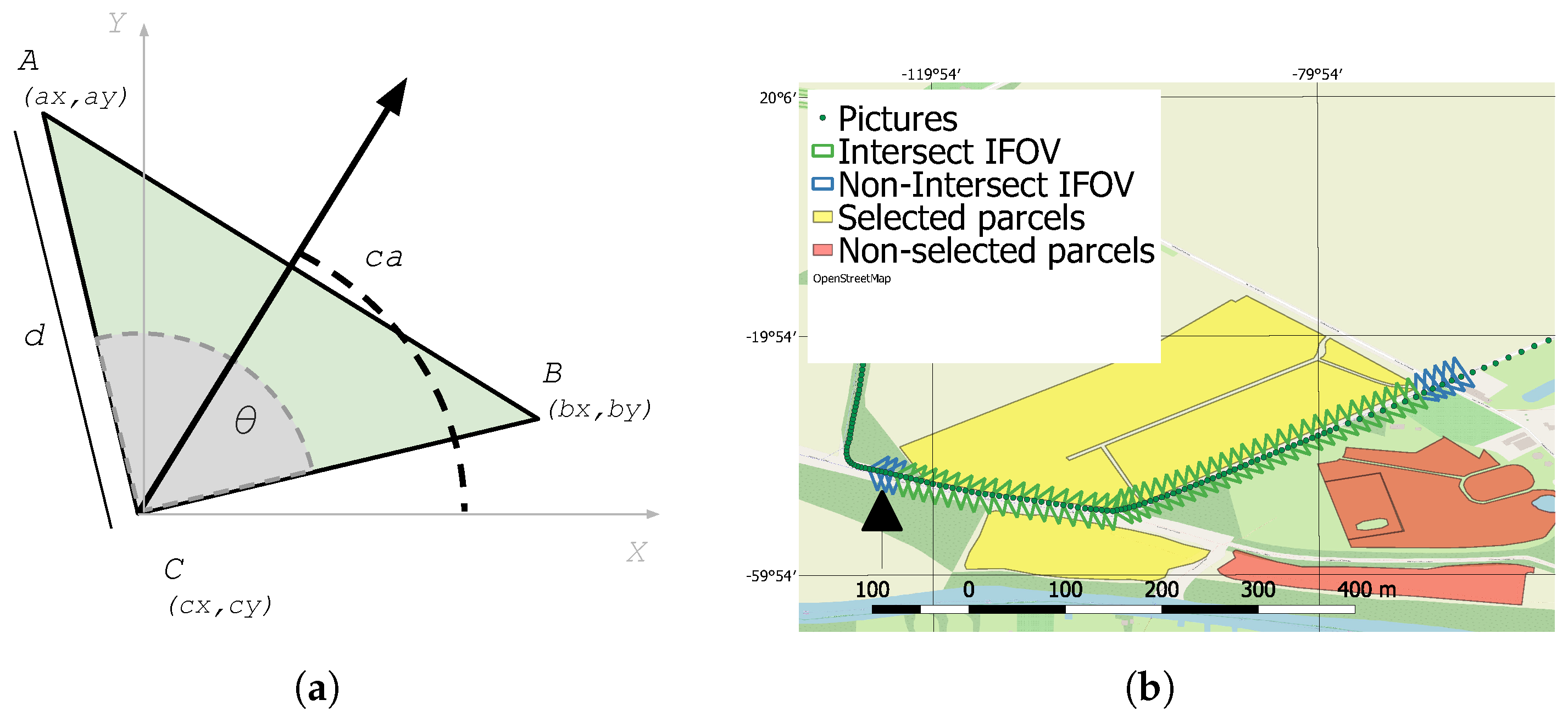
The images were obtained between 2013–2018 and most of them are located in cities; as such only a fraction of these will be useful for our analysis. In order to arrive at meaningful information we create a table, which holds only the images within a 50 m buffer of an agricultural parcel and that have been taken between 2017-01-01 and 2018-01-01. To identify those parcels that are potentially observed by crowdsourced images further selection steps are needed. To do this we developed an automated approach to calculate triangular or circular IFOVs for each image. It is important to remark on the need of projecting all spatial data before calculating the IFOVs, as the distortion that occurs as a result of having the data in the Mapillary-native WGS84 causes the triangular polygons to be of different sizes and shapes. In our case we chose to work in Amersfoort/RD New projection (EPSG:28992). The horizontal angle of view () (in grey in Figure 3a) is obtained via Equation (3) where fixed camera width and height, computed focal length (stored as a ratio of image size and focal distance () (Equation (4))), denotes the maximum value of the two arguments (width and height) and then take the coordinates of the point itself as the central vertex of the triangular IFOV. The (Equation (5)) is the nominal focal length stored in the Exchangeable Image File (EXIF) metadata, recorded in millimeters as the equivalent focal length for a camera with 35 mm film and a width of 36 mm. The x and y coordinates of the other two vertexes A and B are calculated with Equations (6) and (7) respectively where X and Y coordinates for vertex A and B, X and Y coordinate for central vertex, the leg of the triangle in terms of distance between central vertex and other vertexes, camera angle in terms of direction of movement (the black arrow in Figure 3a) and is the camera’s horizontal angle of view.
For the panoramic 360 cameras, we assume the IFOV to be most adequately represented by a circular buffer with a radius of 50 m. Attribute information of each image is appended to each respective corresponding triangular or circular polygon. The last step is to perform a simple intersection between the IFOVs (green and blue triangles in Figure 3b) and the parcels in order to only keep those images whose IFOVs intersect with a parcel. By means of this method, the parcels selected are displayed in yellow, while the ones that are not—are in red (Figure 3b). In this way we ensure to keep only those images, that, to the best of our assumptions, will have the parcel displayed on them. Metadata is stored in a table of polygon features which can easily be queried or exported to a desired format.
4. Results
4.1. Availability Assessment
The spatial availability was assessed over Europe (EU-28). For each LUCAS point, a request was sent to the Mapillary server and the reply was saved. For 37.78% of the LUCAS points, an image was available within their 2 km neighborhood (Table 2) while for 62.16% of the points no image was available in a 2 km buffer. For 0.06% of the points, there was an error in the retrieval: 115 points had a error 504 (Gateway Time-out) and 78 points had an error 502 (Bad Gateway).
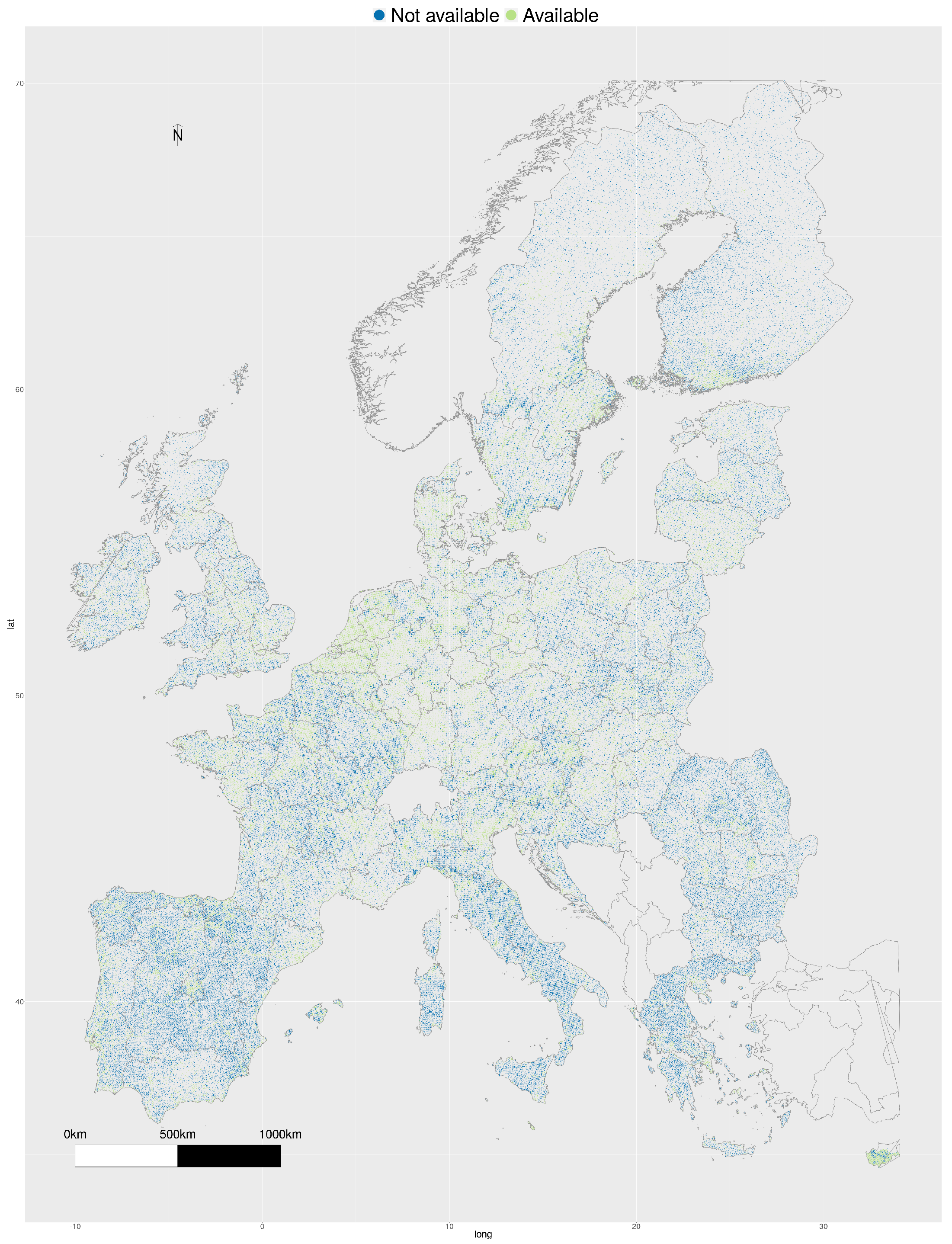
The detailed spatial distribution of the LUCAS points that have at least one crowdsourced image within a distance of 2 km available is mapped in green in Figure 4. LUCAS 2018 points without Mapillary crowdsourced images within a distance of 2 km are shown in blue.
4.1.1. Density Assessment
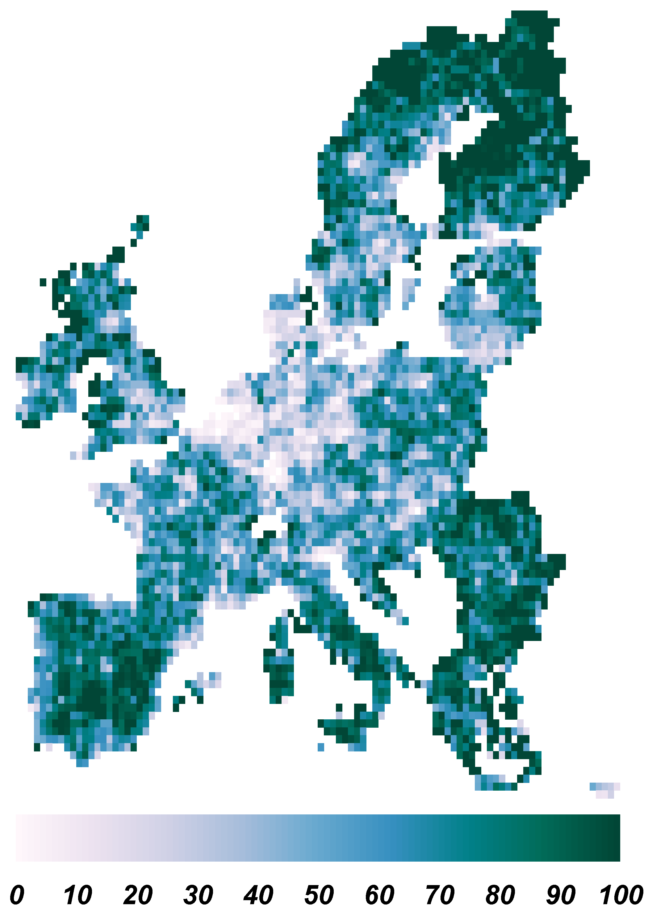
First, the local density is measured using the quadrat density (Figure 5) and demonstrates the heterogeneity of the coverage.
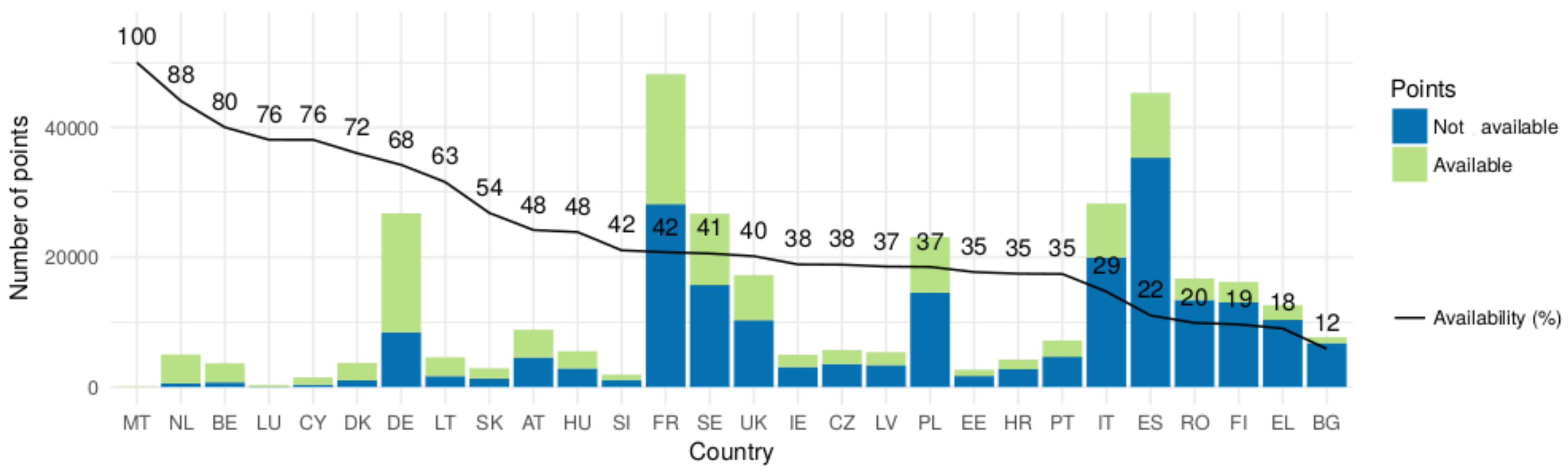
Second, the global density is calculated for each country. Figure 6 provides the detailed availability (%) sorted by country and also provides the number of points for which crowdsourced images are available (green) and not available (blue). The availability ranges from 100% for Malta (MT) to 12% for Bulgaria (BG). However, Malta contains only 79 LUCAS points. The Netherlands has the second highest availability (88%) for a total of 5011 LUCAS points.
Third, the global density was assessed for 8 main land cover classes: Arable land, Permanent crops, Grass, Wooded areas, Shrubs, Bare surface, Artificial areas and Inland water (Table 3), following the LUCAS stratification. Shrubs have the lowest availability (26.94%), while the Artificial areas land cover class has the highest availability of crowdsourced images (63.14%). Arable land has an availability of 40.87%.
4.1.2. Distance Assessment
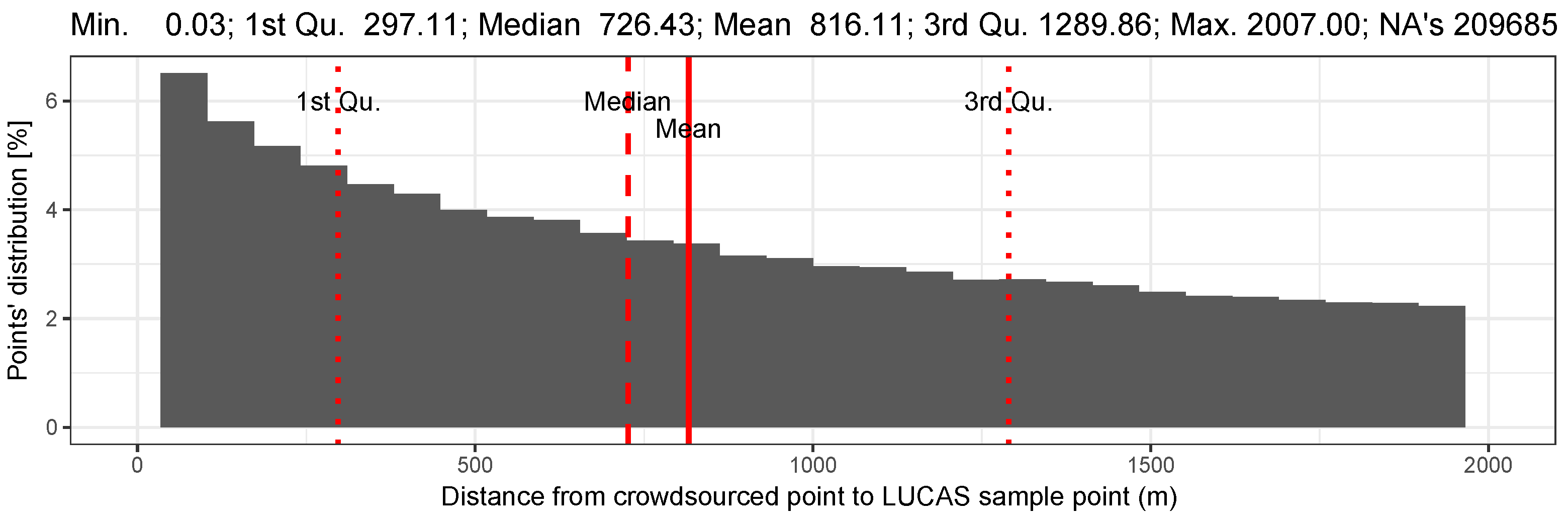
For those LUCAS points for which a crowdsourced image was available (N = 127,346), the distance from the location of the image to the point is of significant interest for this study. The distribution of these distances (Figure 7) indicates that 25% of the images are located within 300 m of the LUCAS point (1st Quartile: 297.11 m), the average distance is 816.11 m.
4.2. Usability Assessment
When assessing usability, we wish to assess the potential of the images to provide a valuable inference for in-situ data. Therefore, we investigated the contributions of Mapillary users, specific attributes from the metadata that we found to be possible benchmarks for image quality, the spatial and temporal distribution of Mapillary data, and finally the parcel revisit rates.
4.2.1. Contributors
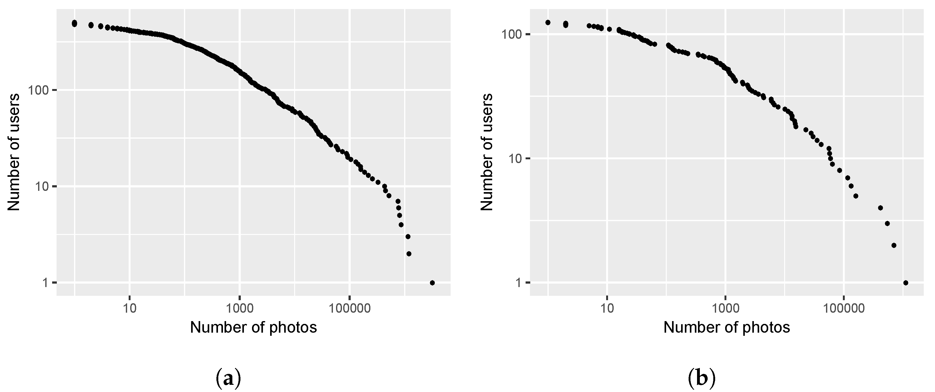
Figure 8 shows the number of images generated as a function of the number of contributors on a logarithmic scale. It is clearly visible that the vast majority of images are generated by a very small community of contributors. In the whole of the Netherlands, 75.15% of all the images are generated by only 1.9% of the contributors (Figure 8a). Indeed most contributors have less than 10 images associated with their user-key, and 68.3% of the contributors have been active on the platform for a total of only one month. For the selected crowdsourced images located at a distance of 50 m to a parcel, a slightly higher percentage of users (4.3%) contributed a similar share of images (73.55%) (Figure 8b). In this subset, skewed to images located in the countryside, the difference between the top contributor and subsequently ranked ones is also smaller compared to the nation-wide dataset.
4.2.2. Metadata Analysis
The meta-data available permits to characterize several quality related aspects of the collected crowdsourced imagery. As a first filter it was necessary to remove images that are suspected of having an inadequate time-stamp. Some 25,093 of the images had a date of creation before the date Mapillary was officially in business. Out of these, 803 are reportedly taken in the 1970s. Suspecting a misrepresentation either due to user oversight when setting the camera clock or issues of translation between date formats, the decision was taken to exclude these. Among the remaining pictures, 16.6% are with a 360 camera. The metadata also contains information [41]. Most of the pictures are looking forward (88.80%) and backward (11.13%), of the remaining pictures, 6370 look right (i.e., 0.05 %) and 3146 look left (i.e., 0.02%).
In terms of camera model, 92 different types of devices have been used to record the images, produced by 33 different vendors. This means that images would undoubtedly vary significantly in terms of usability for potential subsequent analysis. The GPS accuracy is the offset between the target’s recorded and its actual position. This is usually measured in meters, where an acceptable GPS accuracy is between 3.5–5.0 m. The mean offset was found to be around 5.02 m, sufficient for the purposes of the current study focusing on agricultural parcels. That being said, extreme offsets of 1400 m were also recorded and the metric was missing for 50.2% of the images. The compass accuracy represents the compass error measured in yaw angles and can be used to determine moving direction; mean error for the dataset was found to be around 10.3 degrees. This metric was missing for 68.9% of images. The HFOV was obtained as described in the methodology to accurately calculate the IFOV for each image. This is done to get as close as possible to a true representation of what is visible from the sensor when the picture is taken. Bearing in mind that most on-board cameras are placed in a forward looking direction, a large HFOV would be beneficial for monitoring of objects in the near-and-far-peripheral vision range. Logically, this will be where in most cases crops will be located. In our case the HFOV for the images was around 179.9 degrees.
4.2.3. Spatial Availability
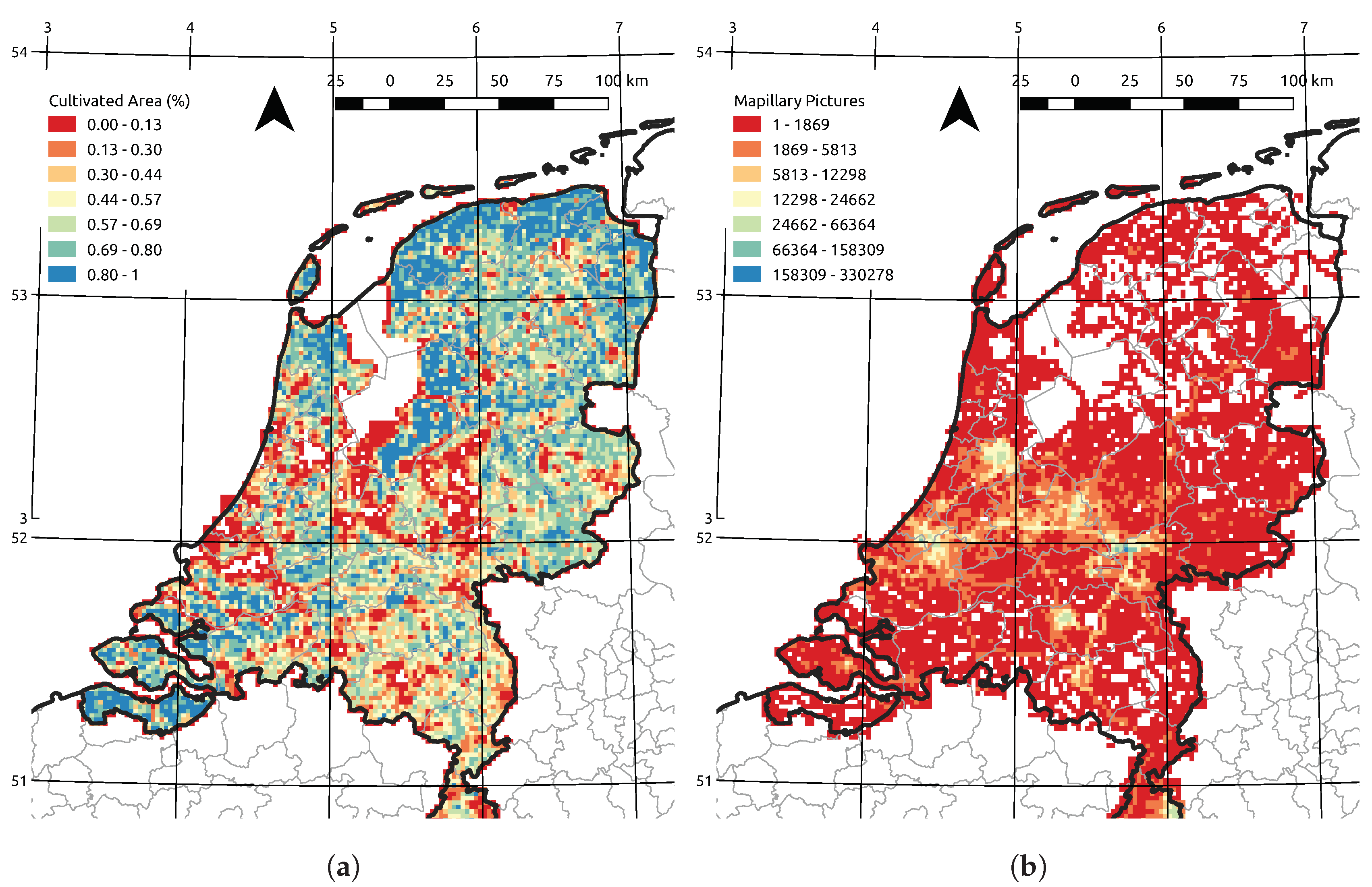
The agricultural land use in the Netherlands, comprising both arable crops and grassland, is aggregated on a 2 km grid as percentage relative to each km grid cell area (Figure 9a): a value of 1 (blue) means that the km grid cell is fully in agricultural land use whereas a value of 0 (red) means that the grid cell is fully covered by something other than agricultural land use. The pattern outlines the major arable production areas, typically on the alluvial soils near the coast, together with large grassland areas on sandy soils and peat areas. These are interspersed with large cities, especially in the western and central parts, and some contiguous nature areas.
For the same km grid, the density of Mapillary pictures was calculated, with high densities in blue and low densities in red (Figure 9b). Grid cells for which no Mapillary pictures are available are left in white. The density scale spans several orders of magnitude, with some of the major urban centres having grid cells with more than 100,000 Mapillary pictures. The correlation coefficient between Mapillary point density and agricultural land use per km grid is −0.172. Furthermore, in major agricultural areas (e.g., in the North and South), most Mapillary pictures are registered along the major road network, leaving significant gaps in the coverage where agricultural land use is most dense.
4.2.4. Temporal Availability
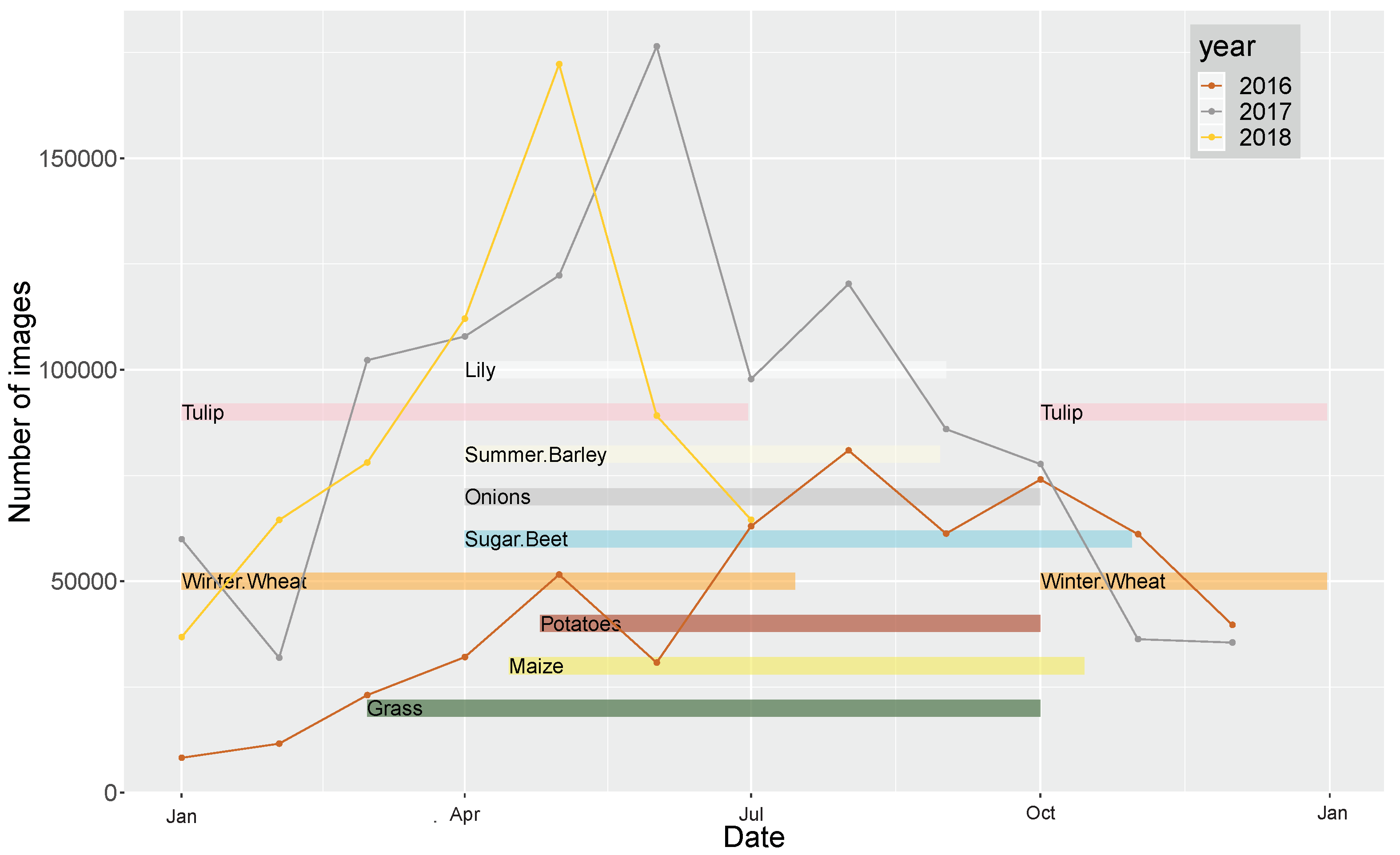
Crop monitoring requires the availability of images throughout the growing season. Multiple re-visits of the same parcel would possibly allow to track crop growth development in that location. Multiple revisits to multiple parcels would allow monitoring crop phenology across climatological gradients. Figure 10 shows the number of images per month for the years 2016, 2017, and 2018, and how these are spread throughout the growing seasons of each crop.
4.2.5. Temporal Availability Targeted to Parcels
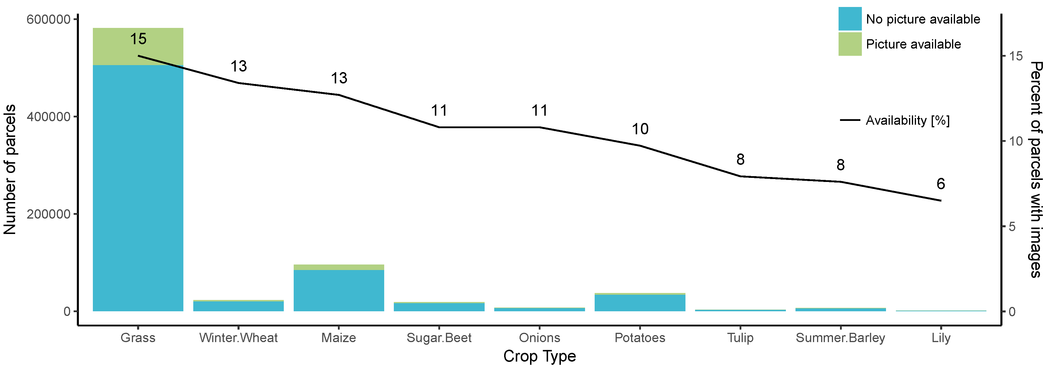
The previous section addresses the general temporal availability of pictures throughout crop specific growing seasons. This section focuses on the parcels of 2017 to analyze parcel specific revisits. First, the parcels that have at least one image associated with them in 2017 are obtained and compared with the total number of parcels in each crop group in 2017 (Figure 11). In 2017, 75,973 grassland parcels have at least 1 observation on a total of 506,183 parcels which corresponds to 15.01%. This availability per crop group range between 15.01% for grasslands to 6.49% for parcels with lilies (availability in black in Figure 11).
Regular repetitive observations of the parcel are a prerequisite to track crop phenological development. The number of unique months for which a given parcel was observed at least once is calculated and then aggregated per crop group resulting in the number of parcels per crop group shown in Table 4. For example, there were 50,249 grassland parcels observed at least once in 2017 representing 9.93% of the parcels while, 12,747 parcels were observed in two different months representing 2.52%. For grassland, 328 parcels were observed each month (representing 0.06%).
One of the eight winter wheat parcels with an observation for each of the 12 months was selected to illustrate the numbers in Table 4. Figure 12 maps all locations of these revisits (Figure 12a), resulting in a high and well-distributed temporal revisit frequency (Figure 12b). Street-level pictures were obtained throughout the seasons (Figure 12c–h). In 2017, the parcel was observed 222 times on 46 unique days, which allows to observe crop development. Pictures taken from nearly the same location were selected to facilitate the comparison. On the right side of the street-level imagery, we can observe the winter wheat growth stages. In January (Figure 12c), the tillering stage could be observed, afterwards the plant is growing and greening (jointing and heading phase, respectively Figure 12d,e). The maturity stage, corresponding to when the plant reaches its maximum height and weight, and starts to become yellow, occurs in summer (Figure 12f,g. In December, the field has been ploughed again (Figure 12h).
5. Discussion
5.1. Availability Assessment
The crowdsourced pictures availability assessment reveals that 37.78% of the EU territory has pictures within 2 km of a LUCAS point (Table 2). The density assessment highlights the heterogeneity of the spatial coverage in the EU. This is confirmed when looking at the global density per country (Figure 6). The availability is above 60% for several countries mainly located in the central north part of the EU (the Netherlands, Belgium, Luxembourg, Denmark and Germany), but also other small countries reach these levels of availability (Malta, Cyprus and Lithuania). In Italy, Spain, Romania, Finland, Greece and Bulgaria, the availability is below 30%. Across all LUCAS land cover classes (Table 3), the artificial area class is ranking highest (63.14%) in global density. Population density is obviously highest in urban areas and people there are proportionally contributing more to the Mapillary platform. Interestingly, for the scope of this paper, the agricultural areas have a rather high global availability over the EU: arable land (40.87%) and permanent crops (36.83%). The LUCAS grid provides statistically reliable figures with a systematic coverage over the EU and a stratified sampling of about 337,031 points. The use of a 2 km buffer to harvest the closest crowdsourced point could be considered a limitation in the study. Obviously, a 2 km distance is often too large to have an actual view on the LUCAS point. However, it was selected as it is the distance between two adjacent LUCAS points. The intention was not to reproduce the LUCAS survey but rather to quantify the spatial distribution and completeness in terms of coverage. In the EU distance assessment (Figure 7), the results show that one quarter of the available crowdsourced points are located less than 300 m from their nearest LUCAS counterpart. Extrapolating this figure with the availability assessment would thus mean that 9.44% (i.e., 25% of 37.78%) of the EU territory has an image within 300 m from a LUCAS point. This assumption illustrates the significant potential of crowdsourcing as a useful and complementary land use and land cover sampling tool.
5.2. Usability Assessment
In the second part of the results, the Dutch Mapillary database was analysed. First, when looking at contributors (Figure 8), more than 75% of the pictures are provided by less than 2% of the users in the Netherlands. Similar results were already demonstrated for Mapillary by [24], and is close to what was demonstrated by [42] where for both Panoramio and Flickr only 1% of the users are responsible for around 70% of the photos taken. This characteristic of the contributing community highlights two contrasting aspects. On the one hand a significant part of the archive (growth) depends on the, voluntary, contributions of relatively few enthusiasts. At the same time, however, creating incentives for these top contributors for specific goals such as using top-end camera equipment, targeted crop monitoring and capture tasking, could lead to significant better quality or more suitable image collection. Understanding the motivation and the purpose of the contributors is therefore key to sustaining this kind of crowdsourced model. For Mapillary, a part of the most active users probably contributes as they believe in open data and user-generated models like Open Street Map. Another potential to increase high-quality thematic contributors could be targeting farmers who commit images with cameras mounted on farm machinery. In this perspective, the EU Code of Conduct on agricultural data sharing [43] provides interesting insights of how this could be organized while respecting at the same time the General Data Protection Regulation (GDPR) [44].
Second, the meta-data analysis demonstrates the heterogeneity of the sensors (92 types of devices from 33 brands). There is still an important potential to exploit the meta-data, including selecting images which orientation meta-data would make them specifically suited for crop monitoring. Indeed, left or right looking images, along with panorama pictures (16.6% of the total) are more suited to retrieve information about crops. The debate on camera position is ongoing in the active Mapillary community [45]. A set of unofficial rules have been articulated to state that users would mostly shoot in a forward looking direction, unless the road has already been mapped this way; or the road is a highway with little change; or when the forward view is obstructed for some reason. Should this type of thinking be adopted more generally throughout the user base, this would mean that when roads get traversed, for example, by active contributors, and mapped in a forward view, subsequent sequences of images on the same road would have the camera positioned to the side. This would generate higher quality images for the purpose of agricultural monitoring.
Third, the detailed spatial availability analysis over the Netherlands (Section 4.2.3) also reveals a heterogeneity in coverage with picture availability negatively correlated to cropland density. Not surprisingly, rural areas have a lower coverage than cities. Furthermore, in rural areas, a larger share of the imagery is collected along the major roads, i.e., at higher average speeds and further away from field boundaries than for imagery collected on local and rural roads and, thus, with reduced quality for crop recognition.
Fourth, considering temporal availability (Section 4.2.4), full representation is lacking as data for 2018 stops in July—the time when the Dutch Mapillary dataset was received. It is still, however, clearly visible that the number of images have significantly increased (by a factor of three) between 2016 and 2017. The incomplete 2018 archive prevents us from confirming this trend for 2018, yet it is encouraging to think that if it does, crowdsourced street-level imagery can become more and more available for crop monitoring or indeed as a source of in-situ information for land use and land cover, and other environmental applications.
Finally, considering parcel specific temporal revisits for 2017 (Section 4.2.5), and specifically the number of parcel observed at least once in 2017 (Figure 11), even if the percentage of parcels observed ranges 6–15%, it still represent a large amount of parcels being observed every year. This is true especially for grasslands, winter wheat, maize and potatoes that cover larger areas. When investigating the number of months for which parcels have observations (Table 4), we observe that, in 2017, the revisit distribution is highly skewed—the vast majority of parcels for all crops have only a single observation. These parcels are thus potentially suited for crop type detection only. The least performing crop in this sense is tulips, with 94% of the parcels visited only once. Parcels with high revisit rates, i.e., at least monthly in the growing season, would be most suited for monitoring of crop phenology. This requirement is often not met, except for the main crops (grassland, maize, potatoes and winter wheat), for which, respectively, 1456, 206, 40 and 24 parcels are observed for five months (Table 4). Furthermore, smart sampling could be designed to take account and make use of inter-field variability to create time-series of regional crop phenology.
5.3. Data Harvesting and Picture Interpretation
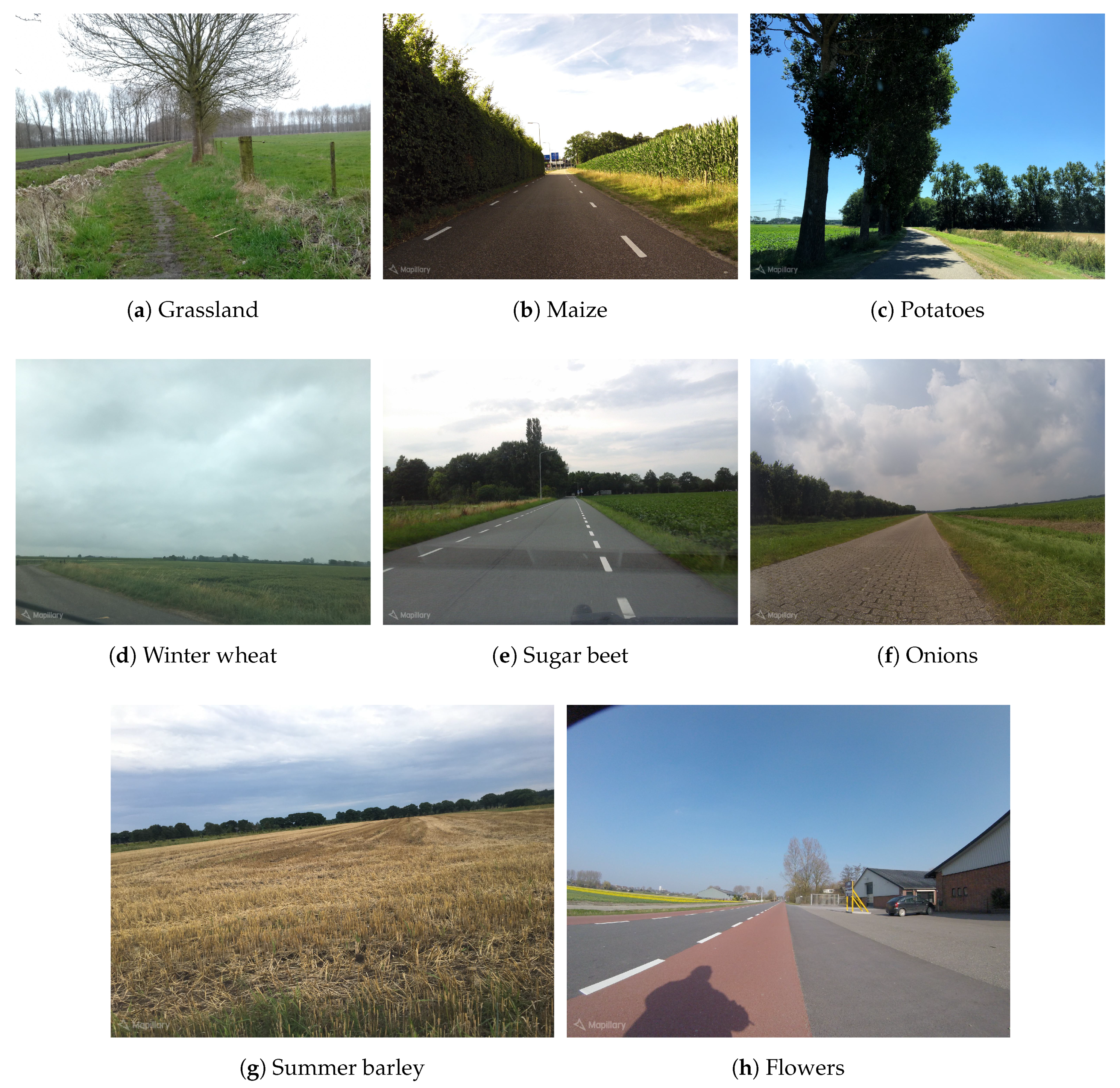
The crop type identification by visual photo-interpretation enables transforming the street-level pictures into information. Figure 13 presents an example of the pictures selected following the geo-spatial analysis to target the best suited pictures. However, many factors including the training of the interpreter, the image quality, the field of view and the parcel size influence the possibility to identify the crop. In [6] we showed that a 90% consistency could be reached among three crop type interpreters, using forward looking street view imagery, though for a limited selection of crop types (grass, maize, cereals) and late in the growing season. Pre-selecting the best quality imagery for visual and later automated interpretation tasks can be further enhanced with sub-image analysis such as perspective segmentation and Mapillary AI tagging of vegetation (and in the future, crops).
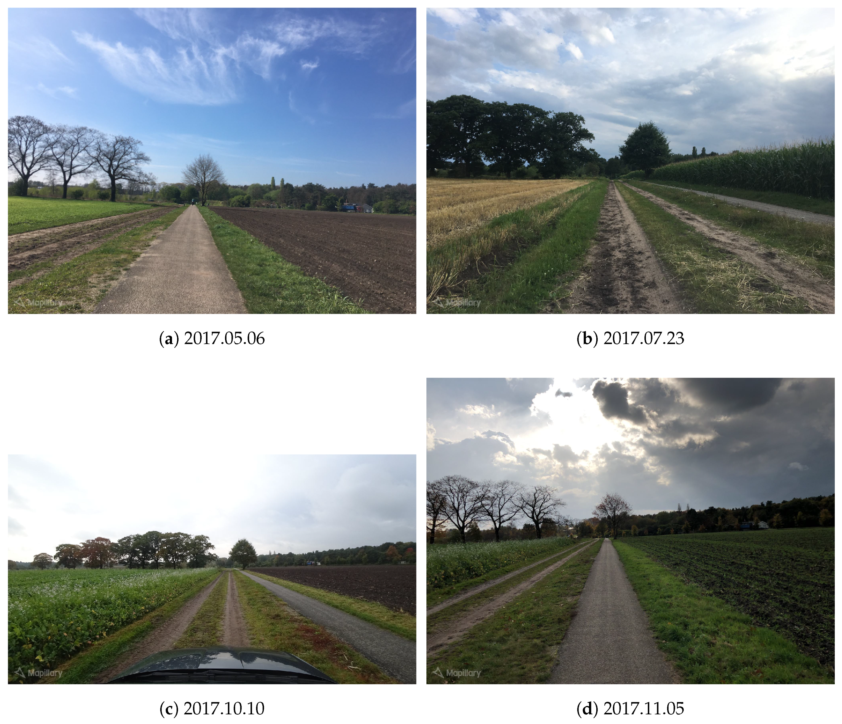
For repetitive image collections, additional logical reasoning may be used, i.e., to pre-condition automatic recognition with the expected sequence of crop phenological states (e.g., flowering in wheat cannot occur before elongation). Even contextual landscape information may be derived directly from the imagery. This is illustrated in Figure 14 which shows a seasonal sequence for two fields. On the left parcel, grass grew (2017.05.06), was harvested (2017.07.23), after which a cover crop was planted (2017.10.10 and 2017.11.05). On the right parcel, the field was recently sown (2017.05.06), maize grew to an advanced stage (2017.07.23), was harvested and the field was ploughed again with some stubble remaining (2017.10.10), and finally the emergence of a winter cereal can be recognized (2017.11.05). The leaf on/leaf off condition of the trees in the background provide some useful indication on the (relative) progress of the season.
Future development of the approach presented here can benefit from existing pheno-cam research [46,47]. Hufkens et al. [47] used cameras to collect near-surface remote sensing data to validate satellite-derived land surface phenology products. Recent developments in Deep Learning should help to automatically extract crop-relevant information from street-level images. Indeed, a few recent studies have used street level imagery for land cover and land use mapping [48,49]. While some challenges still need to be addressed, the proposed approach opens avenues for other applications besides crop type identification such as phenology, flowering, impacts of extreme weather impacts, landscape features, linear elements, hedgerows and monitoring of agricultural activities, e.g., grassland mowing.
5.4. Capture Tasks and Image Quality
Image quality relates to different aspects of the capturing process and the image itself. This determines whether the parcel is going to be visible on the image. Cameras may be out of focus, or placed improperly resulting in visual distortions that hamper image usability. Environmental factors such as sun glint or rain conditions also impact image quality. Concerning improperly placed cameras, the Mapillary tech-team have expressed their eagerness to correct for this by automatic object detection and soft cropping of, for example, dashboards or other car parts that obstruct camera view [50]. Reflections off wind shields, caused by sun glint are among the most commonly reported issues by Mapillary users [51]. Possible proposed solutions to prevent this effect include the use of a Circular Polarized Filter (CPF), for which both industrial and do-it-yourself solutions exist (e.g., use of a lens from 3D glasses). Alternatively, to mitigate already caused damage to the image, recent advances in computer vision allow the exploitation of ghosting cues for layer separation in order to remove the unwanted reflection [52]. Improved cameras (e.g., two stereoscopic cameras, LiDAR, additional spectral bands) could bring new opportunities for vegetation monitoring. For example, Filippa et al. [53] showed that sensors with a Near InfraRed (NIR) spectral channel permit to derive Normalized Difference Vegetation Index (NDVI) to validate satellite phenology products. In the future, dedicated crop capture tasks and use of constantly improving techniques to augment image reliability can improve image quality and expand coverage in rural areas.
The view of the parcel may also be obstructed. For instance, roads are often surrounded by lines of trees or hedges, making it necessary to carry out visual inspection or alternatively add an extra step to the analysis to account for this. Consecutive images taken during the same capture track can help in selecting the image with the best unobstructed view. Additionally, there may be infrastructural visual obstructions, such as embankments or dike ring walls. A possible integration of a high resolution Digital Elevation Model (DEM), such as the Dutch Actueel Hoogtebestand Nederland (AHN) 2017/2018 [54], or Light Detection And Ranging (LiDAR) data could make for an automated mechanism to filter out those images. Automatically selecting images a priori best suited to view a parcel will benefit from further methodological developments (e.g., distance to roads, exclusion of highway pictures, using metadata such as speed to target only observations from bicycles and pedestrians).
6. Conclusions
This study demonstrated the potential of crowdsourced street level imagery as a source of in-situ data for agricultural monitoring. Statistical methods on density and distance were used to measure the availability of crowdsourced images throughout Europe with respect to the LUCAS 2018 sampling grid in terms of both country-wide scale and land cover. A specific case study was done in the Netherlands to evaluate the potential of extracting crop-relevant in-situ data from these images. A detailed methodology to harvest the images potentially best suited to observe a parcel was developed taking advantage of the parcel geometries and crop declarations in the Dutch LPIS. The availability of Mapillary crowdsourced street level imagery throughout the EU and the Netherlands is heterogeneous and challenges to extract useful information from images remain. Nevertheless, potential benefits of extracting in-situ data relevant for crop identification, crop rotation, and crop phenology are presented. Realizing this potential would complement and further valorize frequent and high resolution observations with the Copernicus Sentinels. Harnessing this novel data source provides a unique opportunity to address pressing information needs in the context of food security, commodity markets, environmental monitoring, and support to sustainable agricultural policy design and implementation.
Author Contributions
R.d., M.Y., G.L. and M.v.d.V. conceived, designed, realized the study and wrote the manuscript. J.Y. and K.N. provided the Mapillary data and technical assistance to handle the data.
Funding
This manuscript has received funding from the European Union’s Horizon 2020 research and innovation program under Grant Agreement No. 689812 (LandSense, https://landsense.eu/).
Acknowledgments
The authors would like to thank the three anonymous reviewers for their constructive comments.
Conflicts of Interest
The authors declare no conflict of interest.
Appendix A. Aggregation of the Crops

Table A1.
Aggregation of the crops in 8 main categories.
| Label | Dutch Name (gws_gewas) | Gewas Code | |
|---|---|---|---|
| 0 | grassland (gra) | Grasland, blijvend Grasland, tijdelijk Grasland, natuurlijk. Hoofdfunctie landbouw. Grasland, natuurlijk. Areaal met een natuurbeheertype... Graszaad | 265 266 331 336 383 |
| 1 | maize (mai) | Maïs, snij- Maïs, korrel- Maïs, corncob mix | 259 316 317 |
| 2 | potatoes (pot) | Aardappelen, consumptie Aardappelen, poot- (NAK) Aardappelen, poot- (ABM) Aardappelen, zetmeel | 2014 2015 2016 2017 |
| 3 | winter wheat (wwh) | Tarwe, winter- | 233 |
| 4 | sugar beet (sbt) | Bieten, suiker- | 256 |
| 5 | onions (oni) | Uien, zaai- Uien, poot- en plant- (incl. sjalotten) | 262 1931 |
| 6 | summer barley (sba) | Gerst, zomer- | 236 |
| 7 | flower (flo) | Tulp, bloembollen en -knollen Lelie, bloembollen en -knollen | 1004 1002 |
Appendix B. Mapillary Metadata Description
Table A2.
Description of the available variables on the Mapillary platform.
| Variable | Full Name | Description |
|---|---|---|
| cca | corrected camera angle | corrections to the ca (camera angle) field, introduced either by the users themselves, other users, or Mapillary staff. |
| altitude | GPS altitude | The height above sea level, as recorded by the onboard GPS system. |
| orientation | camera orientation | Seeing as how the vast majority of values for this variable is 1, we assume the following: 1 == landscape orientation, 3 == portrait orientation |
| cfocal | camera focal length | The optical distance from the point where light rays converge |
| camera_mode | camera acquisition mode | The mode of acquiring the images. |
| calt | camera altitude | Camera altitude in terms of how high the camera is positioned from the ground in meters. |
| captured_at | -#- | When the image was captured |
| created_at | -#- | When the image was created |
| user_key | -#- | The unique key identifier for the image/sequence contributor |
| compass_accuracy | digital compass accuracy | Compass error measured in yaw angles. |
| sequence | sequence key | The unique key identifier for the sequence of images |
| gps_accuracy | horizontal GPS accuracy | The offset between the target’s recorded and its actual position. Usually measured in meters (standard GPS accuracy is 3.5–5.0 m.) |
| width | fixed camera width | The x dimension of the image—how many pixels it is wide. |
| fmm35 | focal length 35 mm | Cameras with a focal length of 35 mm. |
| model | camera model | -#- |
| make | made from | The company, producing the cameras |
| ca | camera angle | The looking direction (0–360 degrees) |
| key | -#- | The unique key identifier for the image |
| height | fixed camera height | The y dimension of the image—how many pixels it is tall. |
| cl | ? | Some lat/lon coordinates that are really close to the image coordinates. |
| l | ? | Some lat/lon coordinates that are really close to the image coordinates. |
| file_size | -#- | Size of the file |
| captured_with | application version | The version of the application the images/sequence was captured with |
| gpano | panorama mode | Whether the image was captured in panorama mode or not, along with some specifications about this |
References
- LDV Capital. 5 Year Visual Tech Market Analysis. 2017. Available online: https://cdn.filestackcontent.com/ZXNI76xKSKqqU7JJuahl (accessed on 30 August 2018).
- Dickinson, J.L.; Zuckerberg, B.; Bonter, D.N. Citizen science as an ecological research tool: Challenges and benefits. Annu. Rev. Ecol. Evol. Syst. 2010, 41, 149–172. [Google Scholar] [CrossRef]
- Nationaal Georegister. Basisregistratie Gewaspercelen (BRP). 2017. Available online: http://www.nationaalgeoregister.nl/geonetwork/srv/dut/catalog.search#/metadata/%7B25943e6e-bb27-4b7a-b240-150ffeaa582e%7D (accessed on 24 November 2017).
- Invekos Schläge. Available online: http://gis.bmlfuw.gv.at/wmsgw-ds/?alias=e722906e-e559-4& request=GetDataFeed&id=ae690988-644c-4c25-bdee-bc7d1f4762ee (accessed on 29 November 2017).
- Jordbrugs Analyser: Geoserver Download. 2017. Available online: http://jordbrugsanalyser.dk/downloadside/index.html (accessed on 29 November 2017).
- D’Andrimont, R.; Lemoine, G.; van der Velde, M. Targeted Grassland Monitoring at Parcel Level Using Sentinels, Street-Level Images and Field Observations. Remote Sens. 2018, 10, 1300. [Google Scholar] [CrossRef]
- Gallego, J.; Delincé, J. The European land use and cover area-frame statistical survey. Agric. Surv. Methods 2010, 149–168. [Google Scholar] [CrossRef]
- Eurostat. LUCAS Web Site. 2018. Available online: https://ec.europa.eu/eurostat/web/lucas (accessed on 30 August 2018).
- Kosmala, M.; Crall, A.; Cheng, R.; Hufkens, K.; Henderson, S.; Richardson, A.D. Season spotter: Using Citizen Science to validate and scale plant phenology from near-surface remote sensing. Remote Sens. 2016, 8, 726. [Google Scholar] [CrossRef]
- FotoQuest Go. Available online: http://fotoquest-go.org/ (accessed on 24 November 2017).
- Van der Velde, M.; See, L.; Fritz, S.; Verheijen, F.G.; Khabarov, N.; Obersteiner, M. Generating crop calendars with Web search data. Environ. Res. Lett. 2012, 7, 024022. [Google Scholar] [CrossRef] [Green Version]
- Fritz, S.; See, L.; McCallum, I.; You, L.; Bun, A.; Moltchanova, E.; Duerauer, M.; Albrecht, F.; Schill, C.; Perger, C.; et al. Mapping global cropland and field size. Glob. Chang. Biol. 2015, 21, 1980–1992. [Google Scholar] [CrossRef] [PubMed] [Green Version]
- Minet, J.; Curnel, Y.; Gobin, A.; Goffart, J.P.; Mélard, F.; Tychon, B.; Wellens, J.; Defourny, P. Crowdsourcing for agricultural applications: A review of uses and opportunities for a farmsourcing approach. Comput. Electron. Agric. 2017, 142, 126–138. [Google Scholar] [CrossRef] [Green Version]
- Gebru, T.; Krause, J.; Wang, Y.; Chen, D.; Deng, J.; Aiden, E.L.; Li, F.-F. Using deep learning and google street view to estimate the demographic makeup of the us. arXiv, 2017; arXiv:1702.06683. [Google Scholar]
- Acharya, A.; Fang, H.; Raghvendra, S. Neighborhood Watch: Using CNNs to Predict Income Brackets from Google Street View Images. Available online: http://cs231n.stanford.edu/reports/2017/pdfs/556.pdf (accessed on 18 October 2018).
- Andersson, V.O.; Birck, M.A.; Araujo, R.M. Investigating Crime Rate Prediction Using Street-Level Images and Siamese Convolutional Neural Networks. In Latin American Workshop on Computational Neuroscience; Springer: Berlin, Germany, 2017; pp. 81–93. [Google Scholar]
- Krylov, V.A.; Kenny, E.; Dahyot, R. Automatic Discovery and Geotagging of Objects from Street View Imagery. Remote Sens. 2017, 10, 661. [Google Scholar] [CrossRef]
- Goel, R.; Garcia, L.M.; Goodman, A.; Johnson, R.; Aldred, R.; Murugesan, M.; Brage, S.; Bhalla, K.; Woodcock, J. Estimating city-level travel patterns using street imagery: A case study of using Google Street View in Britain. PLoS ONE 2018, 13, e0196521. [Google Scholar] [CrossRef] [PubMed]
- Iannelli, G.C.; Dell’Acqua, F. Extensive Exposure Mapping in Urban Areas through Deep Analysis of Street-Level Pictures for Floor Count Determination. Urban Sci. 2017, 1, 16. [Google Scholar] [CrossRef]
- Seiferling, I.; Naik, N.; Ratti, C.; Proulx, R. Green streets-Quantifying and mapping urban trees with street-level imagery and computer vision. Landsc. Urban Plan. 2017, 165, 93–101. [Google Scholar] [CrossRef]
- Li, X.; Zhang, C.; Li, W.; Ricard, R.; Meng, Q.; Zhang, W. Assessing street-level urban greenery using Google Street View and a modified green view index. Urban For. Urban Green. 2015, 14, 675–685. [Google Scholar] [CrossRef]
- Long, Y.; Liu, L. How green are the streets? An analysis for central areas of Chinese cities using Tencent Street View. PLoS ONE 2017, 12, e0171110. [Google Scholar] [CrossRef] [PubMed]
- Mapillary. Available online: https://www.mapillary.com/ (accessed on 24 November 2017).
- Juhász, L.; Hochmair, H.H. User contribution patterns and completeness evaluation of Mapillary, a crowdsourced street level photo service. Trans. GIS 2016, 20, 925–947. [Google Scholar] [CrossRef]
- Wu, B.; Li, Q. Crop planting and type proportion method for crop acreage estimation of complex agricultural landscapes. Int. J. Appl. Earth Obs. Geoinf. 2012, 16, 101–112. [Google Scholar] [CrossRef]
- Singha, M.; Wu, B.; Zhang, M. Object-based paddy rice mapping using HJ-1A/B data and temporal features extracted from time series MODIS NDVI data. Sensors 2016, 17, 10. [Google Scholar] [CrossRef] [PubMed]
- USGS. Global Croplands Street View Application. Available online: https://www.croplands.org/app/data/street (accessed on 27 March 2018).
- Xiong, J.; Thenkabail, P.S.; Gumma, M.K.; Teluguntla, P.; Poehnelt, J.; Congalton, R.G.; Yadav, K.; Thau, D. Automated cropland mapping of continental Africa using Google Earth Engine cloud computing. ISPRS J. Photogramm. Remote Sens. 2017, 126, 225–244. [Google Scholar] [CrossRef]
- Mapillary. First Photo Day—A Look at Two Years of Mapillary—The Mapillary Blog. 2015. Available online: https://blog.mapillary.com/update/2015/10/08/twoyears.html (accessed on 30 August 2018).
- Mapillary. 100 Million Photos—Geotagged, Connected, and Available for All—The Mapillary Blog. 2016. Available online: https://blog.mapillary.com/update/2016/11/15/100-million-photos-geotagged-connected-and-available-for-all.html (accessed on 30 August 2018).
- Mapillary. Celebrating 200 Million Images—The Mapillary Blog. 2017. Available online: https://blog.mapillary.com/update/2017/10/05/200-million-images.html (accessed on 30 August 2018).
- HERE and Mapillary: Linking Two Global Communities—The Mapillary Blog. 2018. Available online: https://blog.mapillary.com/update/2018/05/10/here-mapillary-global-partnership.html (accessed on 30 August 2018).
- Juhász, L.; Hochmair, H.H. Cross-linkage between Mapillary street level photos and OSM edits. In Geospatial Data in a Changing World; Springer: Berlin, Germany, 2016; pp. 141–156. [Google Scholar]
- Reuters, T. Sweden’s Mapillary Raises $15 Million in Funding Round led by BMW i Ventures. 2018. Available online: https://www.reuters.com/article/mapillary-fundraising/swedens-mapillary-raises-15-million-in-funding-round-led-by-bmw-i-ventures-idUSL8N1RN4YL (accessed on 30 August 2018).
- Creative Commons. Creative Commons—Attribution-ShareAlike 4.0 International—CC BY-SA 4.0. Available online: https://creativecommons.org/licenses/by-sa/4.0/ (accessed on 30 August 2018).
- Mapillary. Mapillary API Documentation—Version 3. 2018. Available online: https://www.mapillary.com/developer/api-documentation/ (accessed on 30 August 2018).
- ESTAT (E4.LUCAS). LUCAS2018: Technical Reference Document S1 Stratification Guidelines. 2018. Available online: http://ec.europa.eu/eurostat/documents/205002/7329820/LUCAS2018_S1-StratificationGuidelines_20160523.pdf (accessed on 8 January 2018).
- JRC. Wikicap—European Commission. Available online: https://marswiki.jrc.ec.europa.eu/wikicap/index.php/Main_Page (accessed on 24 November 2017).
- Gillies, S.; Butler, H.; Daly, M.; Doyle, A.; Schaub, T. The GeoJSON Format. Coordinates 2016, 102. [Google Scholar] [CrossRef]
- Sinnott, R.W. Virtues of the Haversine. Sky Telesc. 1984, 68, 159. [Google Scholar]
- Jpegcrop. Exif Orientation Tag. 2002. Available online: http://sylvana.net/jpegcrop/exif_orientation.html (accessed on 13 September 2018).
- Alivand, M.; Hochmair, H.H. Spatiotemporal analysis of photo contribution patterns to Panoramio and Flickr. Cartogr. Geogr. Inf. Sci. 2017, 44, 170–184. [Google Scholar] [CrossRef]
- COPA-COGECA. EU Code of Conduct on Agricultural Data Sharing by Contractual Arrangement. 2018. Available online: http://cema-agri.org/sites/default/files/publications/EU_Code_2018_web_version.pdf (accessed on 21 September 2018).
- European Union. Regulation (EU) 2016/679 of the European Parliament and of the Council of 27 April 2016 on the protection of natural persons with regard to the processing of personal data and on the free movement of such data, and repealing Directive 95/46/EC (General Data Protection Regulation). Off. J. Eur. Union 2016, L119, 1–88. [Google Scholar]
- Mapillary Forum. Regarding ‘Capturing’ Sideways Instead of Roads. 2016. Available online: https://forum.mapillary.com/t/regarding-capturing-sideways-instead-of-roads/1444/2 (accessed on 26 September 2018).
- Vrieling, A.; Meroni, M.; Darvishzadeh, R.; Skidmore, A.K.; Wang, T.; Zurita-Milla, R.; Oosterbeek, K.; O’Connor, B.; Paganini, M. Vegetation phenology from Sentinel-2 and field cameras for a Dutch barrier island. Remote Sens. Environ. 2018, 215, 517–529. [Google Scholar] [CrossRef]
- Hufkens, K.; Friedl, M.; Sonnentag, O.; Braswell, B.H.; Milliman, T.; Richardson, A.D. Linking near-surface and satellite remote sensing measurements of deciduous broadleaf forest phenology. Remote Sens. Environ. 2012, 117, 307–321. [Google Scholar] [CrossRef]
- Kang, J.; Körner, M.; Wang, Y.; Taubenböck, H.; Zhu, X.X. Building instance classification using street view images. ISPRS J. Photogramm. Remote Sens. 2018, 145, 44–59. [Google Scholar] [CrossRef]
- Zhu, Y.; Deng, X.; Newsam, S.D. Fine-Grained Land Use Classification at the City Scale Using Ground-Level Images. arXiv, 2018; arXiv:1802.02668. [Google Scholar]
- Mapillary Forum. Suggestions for Computer Vision Features. 2015. Available online: https://forum.mapillary.com/t/suggestions-for-computer-vision-features/58 (accessed on 28 September 2018).
- Mapillary Forum. Reducing Dashboard Reflections with a CPL (Circular Polarizer Filter). 2015. Available online: https://forum.mapillary.com/t/reducing-dashboard-reflections-with-a-cpl-circular-polarizer-filter/174 (accessed on 28 September 2018).
- Shih, Y.; Krishnan, D.; Durand, F.; Freeman, W.T. Reflection removal using ghosting cues. In Proceedings of the IEEE Conference on Computer Vision and Pattern Recognition, Boston, MA, USA, 7–12 June 2015; pp. 3193–3201. [Google Scholar]
- Filippa, G.; Cremonese, E.; Migliavacca, M.; Galvagno, M.; Sonnentag, O.; Humphreys, E.; Hufkens, K.; Ryu, Y.; Verfaillie, J.; di Cella, U.M.; et al. NDVI derived from near-infrared-enabled digital cameras: Applicability across different plant functional types. Agric. For. Meteorol. 2018, 249, 275–285. [Google Scholar] [CrossRef]
- AHN. AHN Netherlands 0.5m DEM, Non-Interpolated. Available online: http://www.ahn.nl/common-nlm/open-data.html (accessed on 20 September 2018).
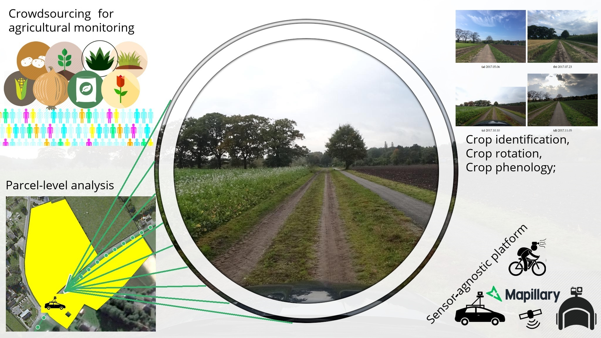
Figure 1.
The first objective of the paper is to assess the spatial availability of crowdsourced street-level imagery data across the European Union (EU-28) based on the Land Use and land Cover Area frame Survey (LUCAS). The second, third, and fourth, objectives are to assess the potential usability of such images to generate in-situ data relevant for crop monitoring in the Netherlands (NL) using to the Dutch agricultural parcel registry, i.e., Basisregistratie Gewasparcelen (BRP).

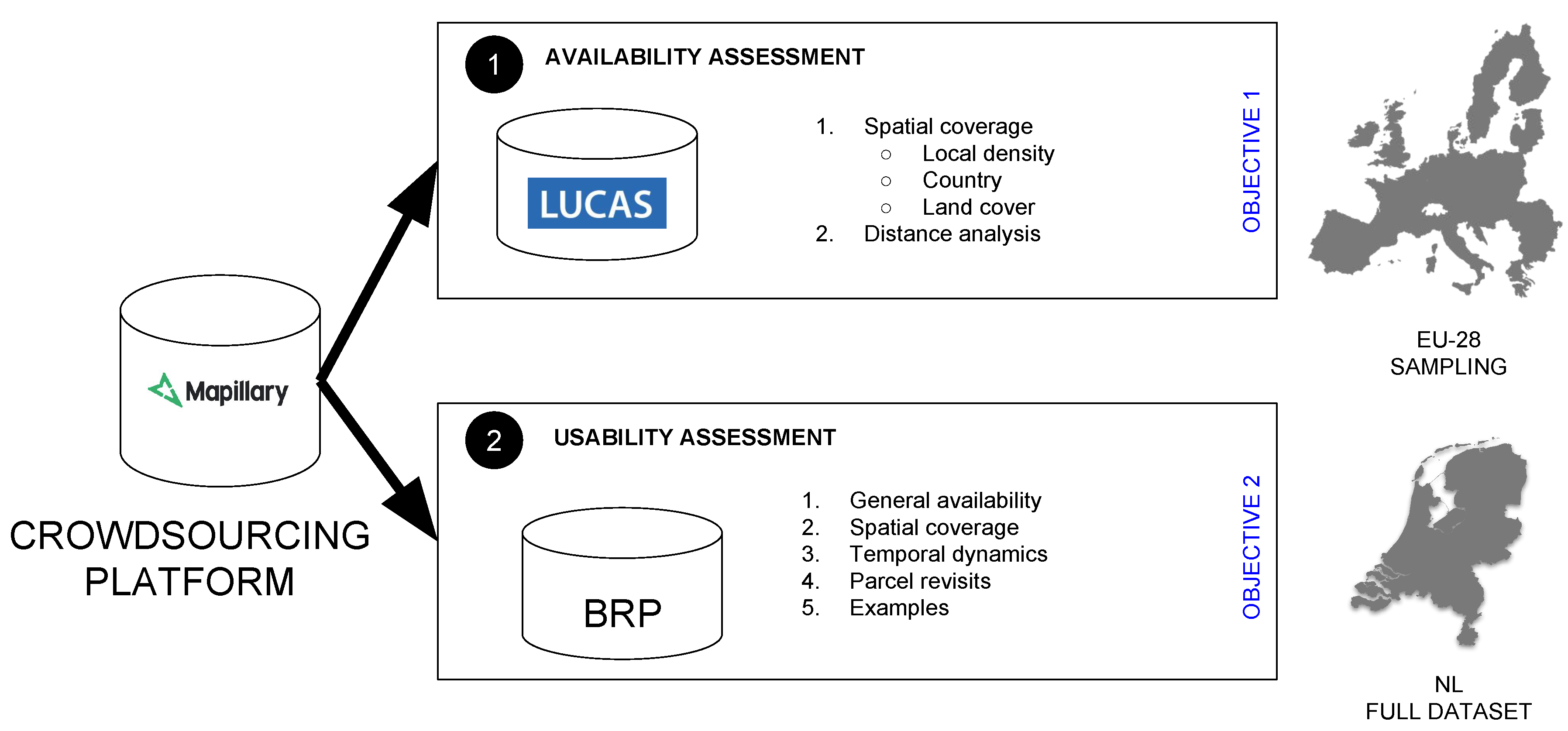
Figure 2.
Methodological flowchart of the availability and usability assessment for Mapillary images in the Netherlands.
Figure 2.
Methodological flowchart of the availability and usability assessment for Mapillary images in the Netherlands.

Figure 3.
The Instantaneous Field Of View (IFOV, green triangle Figure 3a from the point where the picture was taken (C) is obtained by calculating the triangle coordinates based on the picture’s metadata. The camera angle (CA) is the moving direction of the sensor. The horizontal angle of view () represented in grey is the azimuth field of view of the camera and thus varies according to the sensor. Figure 3b shows the process of intersecting the generated (in this case triangular) IFOVs with the parcel boundaries, leading to parcel selection (yellow) or not (red).

Figure 4.
Map displaying the LUCAS 2018 survey points. To assess the availability of Mapillary crowdsourced steet-level imagery, the location with a crowdsourced image closest to each of the 337,031 LUCAS points was harvested through the Mapillary API. The LUCAS points for which an image was available within a 2 km distance are represented in green (N = 127,346 representing 37.78% of the total) while the points without a crowdsourced image within a 2 km buffer are represented in blue (N = 209,492 representing 62.16%).

Figure 5.
Local density of available street-level imagery within a 2 km radius of LUCAS 2018 points based on a systematic spatial sampling of 337,031 points averaged by grid cell (%).
Figure 5.
Local density of available street-level imagery within a 2 km radius of LUCAS 2018 points based on a systematic spatial sampling of 337,031 points averaged by grid cell (%).

Figure 6.
Density by country sorted from the largest availability to the lowest. The bar plot shows the number of LUCAS points for which crowdsourced data are available (green) and not available (blue) summarized by country. The availability (%) is represented by the black line.
Figure 6.
Density by country sorted from the largest availability to the lowest. The bar plot shows the number of LUCAS points for which crowdsourced data are available (green) and not available (blue) summarized by country. The availability (%) is represented by the black line.

Figure 7.
Distribution of the distances between LUCAS points and the locations of the closest crowdsourced image.
Figure 7.
Distribution of the distances between LUCAS points and the locations of the closest crowdsourced image.

Figure 8.
Distribution of user-generated images for (a) the entire Dutch Mapillary dataset and (b) for the photos within a 50-m buffer of an agricultural parcel.
Figure 8.
Distribution of user-generated images for (a) the entire Dutch Mapillary dataset and (b) for the photos within a 50-m buffer of an agricultural parcel.

Figure 9.
The proportion of agricultural land use in a 2 km grid over the Netherlands (a) shows the areas where data are needed for crop monitoring. The Mapillary data availability for agricultural parcels is aggregated for the same 2 km grid and shows a heterogeneous pattern (b).
Figure 9.
The proportion of agricultural land use in a 2 km grid over the Netherlands (a) shows the areas where data are needed for crop monitoring. The Mapillary data availability for agricultural parcels is aggregated for the same 2 km grid and shows a heterogeneous pattern (b).

Figure 10.
Monthly availability of images throughout the year for 2016–2018 along with growing season of the main crops.
Figure 10.
Monthly availability of images throughout the year for 2016–2018 along with growing season of the main crops.

Figure 11.
Number of parcels observed and not observed at least once in 2017 per crop group. The crop groups are ordered by the proportion of parcels having at least one picture in 2017 to the total number of parcels (availability).
Figure 11.
Number of parcels observed and not observed at least once in 2017 per crop group. The crop groups are ordered by the proportion of parcels having at least one picture in 2017 to the total number of parcels (availability).

Figure 12.
In 2017, this parcel (latitude = 51.9567 N, longitude = 5.6345 E) was observed 222 times on 46 unique days. The average revisit rate is 4.8 days. Having frequent pictures permits to observe several winter wheat growth stages.
Figure 12.
In 2017, this parcel (latitude = 51.9567 N, longitude = 5.6345 E) was observed 222 times on 46 unique days. The average revisit rate is 4.8 days. Having frequent pictures permits to observe several winter wheat growth stages.

Figure 13.
Street-level imagery permit to identify crop label by visual interpretation.

Figure 14.
On the left parcel grass was followed by a cover crop, on the right parcel, maize was followed by a winter cereal. Also note the leaf on/leaf off condition of the trees in the background, which provides seasonal context. (latitude = 51.9922 N,longitude = 5.7421 E).
Figure 14.
On the left parcel grass was followed by a cover crop, on the right parcel, maize was followed by a winter cereal. Also note the leaf on/leaf off condition of the trees in the background, which provides seasonal context. (latitude = 51.9922 N,longitude = 5.7421 E).

Table 1.
Aggregated crop classes and their respective growing season.
| Aggregated Crop Class | Growing Season | Percentage of Total Area |
|---|---|---|
| Grassland | March—October | 64.42% |
| Maize | mid April—mid October | 10.83% |
| Potatoes | late April—October | 4.34% |
| Winter Wheat | Autumn—mid July * | 2.60% |
| Sugar Beet | early April—late October | 2.18% |
| Onions | April—October | 0.85% |
| Summer Barley | April—late August | 0.80% |
| Flowers—Tulip | October—late June | 0.58% |
| Flowers—Lilly | Spring—September |
* if soft wheat.
Table 2.
Global density of LUCAS points with and without Mapillary crowdsourced images within a 2 km distance. The retrieval errors are mainly network errors due to server failures (502, 504).
Table 2.
Global density of LUCAS points with and without Mapillary crowdsourced images within a 2 km distance. The retrieval errors are mainly network errors due to server failures (502, 504).
| Number | Percent (%) | |
|---|---|---|
| LUCAS 2018 points with a crowdsourced image within a 2 km radius | 127,346 | 37.78 |
| LUCAS 2018 points without a crowdsourced in a 2 km radius | 209,492 | 62.16 |
| Retrieval errors | 193 | 0.06 |
| Total | 337,031 | 100 |
Table 3.
Availability of crowdsourced imagery based on the LUCAS sampling for 8 main land cover strata.
Table 3.
Availability of crowdsourced imagery based on the LUCAS sampling for 8 main land cover strata.
| Strata Description | Corresponding Classes | Available | Unavailable | Total | Global Availability Per Stratum (%) |
|---|---|---|---|---|---|
| Arable land | Cereals, root crops, non-permanent industrial crops, dried pulses, vegetables and flowers, fodder crops | 45,740 | 66,172 | 111,912 | 40.87 |
| Permanent crops | Fruit trees and fruit bushes, other permanent crops (vineyards, olive trees) | 1384 | 2374 | 3758 | 36.83 |
| Grass | Grassland, with or without sparse tree/shrub cover | 19,970 | 32,848 | 52,818 | 37.81 |
| Wooded areas | Areas where at least 10% is covered by tree | 40,416 | 83,104 | 123,520 | 32.72 |
| Shrubs | Shrub land with or without sparse tree cover | 5495 | 14,903 | 20,398 | 26.94 |
| Bare surface, rare or low vegetation | Bare land: areas with no vegetation (rocks, sand, and lichens) or areas covered less than 10% by dominant species of vegetation. | 948 | 1847 | 2795 | 33.92 |
| Artificial, construction and sealed areas | Built-up and artificial non built-up areas | 12,517 | 7307 | 19,824 | 63.14 |
| Inland water | Surfaces covered by water or ice, either permanently or for most of year | 876 | 1130 | 2006 | 43.67 |
Table 4.
Number of parcels and their monthly revisit frequency for each crop group.
| Number of Month | 1 | 2 | 3 | 4 | 5 | 6 | 7 | 8 | 9 | 10 | 11 | 12 |
|---|---|---|---|---|---|---|---|---|---|---|---|---|
| Grass | 50,249 (9.93%) | 12,747 (2.52%) | 4917 (0.97%) | 2411 (0.48%) | 1456 (0.29%) | 1006 (0.2%) | 673 (0.13%) | 455 (0.09%) | 758 (0.15%) | 571 (0.11%) | 402 (0.08%) | 328 (0.06%) |
| Maize | 6989 (8.21%) | 1731 (2.03%) | 588 (0.69%) | 340 (0.4%) | 206 (0.24%) | 204 (0.24%) | 128 (0.15%) | 109 (0.13%) | 211 (0.25%) | 112 (0.13%) | 96 (0.11%) | 78 (0.09%) |
| Potatoes | 2467 (7.23%) | 471 (1.38%) | 159 (0.47%) | 72 (0.21%) | 40 (0.12%) | 39 (0.11%) | 4 (0.01%) | 16 (0.05%) | 15 (0.04%) | 14 (0.04%) | 9 (0.03%) | 7 (0.02%) |
| Winter Wheat | 2001 (9.76%) | 406 (1.98%) | 124 (0.6%) | 59 (0.29%) | 24 (0.12%) | 43 (0.21%) | 15 (0.07%) | 33 (0.16%) | 20 (0.1%) | 12 (0.06%) | 5 (0.02%) | 8 (0.04%) |
| Sugar Beet | 1318 (7.66%) | 300 (1.74%) | 76 (0.44%) | 34 (0.2%) | 28 (0.16%) | 28 (0.16%) | 13 (0.08%) | 22 (0.13%) | 15 (0.09%) | 8 (0.05%) | 8 (0.05%) | 4 (0.02%) |
| Onions | 558 (8.28%) | 105 (1.56%) | 29 (0.43%) | 17 (0.25%) | 4 (0.06%) | 8 (0.12%) | 1 (0.01%) | 1 (0.01%) | 1 (0.01%) | 2 (0.03%) | 1 (0.01%) | 2 (0.03%) |
| Summer Barley | 327 (5.16%) | 75 (1.18%) | 32 (0.5%) | 9 (0.14%) | 8 (0.13%) | 6 (0.09%) | 4 (0.06%) | 11 (0.17%) | 3 (0.05%) | 1 (0.02%) | - | 6 (0.09%) |
| Flowers | 265 (5.75%) | 41 (0.89%) | 15 (0.33%) | 11 (0.24%) | 8 4 (0.09%) | 5 (0.11%) | - | - | 1 (0.02%) | - | 1 (0.02%) | - |
© 2018 by the authors. Licensee MDPI, Basel, Switzerland. This article is an open access article distributed under the terms and conditions of the Creative Commons Attribution (CC BY) license (http://creativecommons.org/licenses/by/4.0/).
Share and Cite
MDPI and ACS Style
D'Andrimont, R.; Yordanov, M.; Lemoine, G.; Yoong, J.; Nikel, K.; Van der Velde, M. Crowdsourced Street-Level Imagery as a Potential Source of In-Situ Data for Crop Monitoring. Land 2018, 7, 127. https://doi.org/10.3390/land7040127
AMA Style
D'Andrimont R, Yordanov M, Lemoine G, Yoong J, Nikel K, Van der Velde M. Crowdsourced Street-Level Imagery as a Potential Source of In-Situ Data for Crop Monitoring. Land. 2018; 7(4):127. https://doi.org/10.3390/land7040127
Chicago/Turabian StyleD'Andrimont, Raphaël, Momchil Yordanov, Guido Lemoine, Janine Yoong, Kamil Nikel, and Marijn Van der Velde. 2018. "Crowdsourced Street-Level Imagery as a Potential Source of In-Situ Data for Crop Monitoring" Land 7, no. 4: 127. https://doi.org/10.3390/land7040127
Note that from the first issue of 2016, this journal uses article numbers instead of page numbers. See further details here.