Modelling Land Sharing and Land Sparing Relationship with Rural Population in the Cerrado


Earth System Science Centre/National Institute for Space Research (CCST/INPE), Avenida dos Astronautas, São José dos Campos 12227-600, Brazil
*
Author to whom correspondence should be addressed.
Land 2018, 7(3), 88; https://doi.org/10.3390/land7030088
Submission received: 19 June 2018
/
Revised: 16 July 2018
/
Accepted: 19 July 2018
/
Published: 21 July 2018
(This article belongs to the Special Issue Land Use and Food Systems Interactions in South America)
Abstract
:Agricultural expansion and intensification enabled growth of food production but resulted in serious environmental changes. In light of that, debates concerning sustainability in agriculture arises on scientific literature. Land sharing and land sparing are two opposite models for framing agricultural sustainability. The first aims to integrate agricultural activities with biodiversity conservation by means of enhancing the quality of the agricultural matrix in the landscape towards a wildlife friendly matrix. The other model aims to spare natural habitats from agriculture for conservation. This work aimed to explore spatial evidences of land sharing/sparing and its relationship with rural population in the Brazilian Cerrado. A Land Sharing/Sparing Index based on TerraClass Cerrado map was proposed. Spatial analysis based on Global and Local Moran statistics and Geographically Weighted Regression were made in order to explore the influence of local rural population on the probability of spatial land sharing/sparing clusters occurrence. Spatial patterns of land sharing were found in the Cerrado and a positive association with rural population was found in some regions, such as in its northern portion. Land use policies should consider regional infrastructural and participative governance potentialities. The results suggests possible areas where joint agricultural activities and human presence may be favourable for biodiversity conservation.
1. Introduction
By the year 2000, more than 55% of the Earth’s ice-free land was occupied by human activities, such as settlements, croplands and pasturelands [1], where about half, one-tenth and one-fifth of those areas are respectively under medium, intense or extensive human management [2]. Altogether, agriculture covers approximately 40% of terrestrial surface, the largest land use on the planet [3]. Expansion of agriculture areas during the last three centuries, combined with increasing yields, enabled substantial growth of food production, but resulted in serious environmental changes [4]. Habitat loss and fragmentation lead to high rates of species extinction [5] and a quarter of anthropogenic Greenhouse Gases (GHG) emissions are related to agricultural activities [6]. In addition, the rising use of pesticides threats both human and non-human populations [7,8,9].
The rapid increase in energy consumption lead to biofuels crops as a renewable and alternative source to fossil fuels, being about 2% of the current global cropland meant for biofuels [10]. Although [11] argues that net expansion of biofuel production is not associated with decline in available area for food production, indirect land use changes caused by biofuel expansion can both negate its GHG savings and lead to the conversion of more forests and savannah to agriculture [12].
In light of the impacts of agriculture to the Earth System, some proposals are made in the scientific literature in order to achieve sustainability in agriculture and reduce its impacts. Two major models under development to frame this issue are the “sustainable intensification of agriculture” model and the “high quality matrix” model or “wildlife-friendly farming”. The former is based on the idea that increasing agricultural yields on already existing farmlands with no additional pressure for clearing new lands will reduce adverse environmental impacts [13,14,15]. This model is also called “land sparing” because large patches of unmanaged environments are separated from high-yield agricultural areas, aiming its protection and biological conservation [16]. The other model, also known as “land sharing”, implies in integrating agricultural activities with areas of high biodiversity, forming complex landscapes with a variety of land uses, which may be suitable for both food production and wildlife habitat [17,18,19,20].
Support information for both land sparing and land sharing models can be widely found in conservation biology, land use and agronomic literature [21,22,23,24,25,26,27,28,29] being the suitability of each model dependent on the landscape’s inherent biophysical properties and its historical, social, cultural and economic context [30,31,32].
Scale also matters in the sharing/sparing debate [31,33]. According to [34] there is a conceptual range of scales at which conservation of biodiversity and agriculture can be integrated, where land sparing and land sharing are the endpoints of this range. In the land sharing strategy, spatial patterns of land cover diversity are detected at finer scales, while in the land sparing model the patches of both agriculture and unmanaged environments are larger and so, the scales of the processes are coarser. Despite these models are spatially antagonistic at the landscape scale, their concomitant analysis provide insights about the intensity and impact of regional human-environmental interactions in a certain landscape, under specific land use trajectories and, current and future, provision of ecosystem services.
In general, studies favouring the sparing strategy are focused on biodiversity [35]. For example, reference [36] argued that the increase rate of big cats populations in China were due to the adoption of land sparing. Also, reference [37] argues that the abundance and species richness of birds, dung beetles and ants in Borneo are higher under land sparing logging. Conversely, references [23,38] claim that wildlife-friendly farming support both high yields and biodiversity. All of these studies used species and yield data from plots or statistical agencies to draw their experiments on the benefits of one or another strategy. The approach presented here, instead, is focused on the actual land use of an entire region with multiple landscape management possibilities.
However, little or no attention is given to local rural populations in most of the studies concerning land sharing and land sparing, as their focus are primarily on agriculture yields, biodiversity conservation and ecosystem services maintenance. Some authors claim that the separation of people from natural areas with little or no human interventions may be one cause of biodiversity loss, therefore local people should be considered as important actors for biodiversity conservation [39,40]. In contrast, reference [41] argues that biological conservation is achieved by rural to urban migration, which leads to farm abandonment and vegetation recovery, as observed in some regions in Central America, and it also represents less potential for expanding agriculture activities over unmanaged natural areas. According to this idea, the reduction of rural population will make more land available for vegetation recovery and conservation, at the same time mechanization over large areas of single crops replaces human working force more efficiently [22,41,42,43]. Despite increased land availability, working force replacement might cause land concentration and speculation, causing further deforestation, as well as off-farm migration into marginal urban areas usually with higher food insecurity [44,45].
On the other hand, wildlife-friendly landscapes with agriculture may be favoured by the presence of smallholders agroecosystems [46,47,48], forming a complex social-ecological system [49] where ecological relationships between unmanaged ecosystems and agriculture is highly relevant [17,50,51,52]. Thus, land sharing offers possibilities and challenges for rural populations of small and family farmers to act towards biological conservation and food production at the same time [53].
In this sense, we followed the hypothesis that at a given agricultural landscape where the rural population density is low, that landscape shall probably have a land use pattern more oriented to the land sparing model [41,43]. Conversely, the higher the rural population density the higher shall be the amount of land sharing observed. For testing this assumption, we developed a spatial explicit Land Sharing/Sparing Index for agricultural landscapes, based on land use and land cover of a region.
Hence, the aim of this study was to develop a Land Sharing/Sparing index at landscape scale and modelling the spatial evidences of land sharing/sparing with rural population density in the Brazilian Cerrado. Land use and land cover in agricultural landscapes in the Cerrado and census tract data were integrated by means of Geographic Information System (GIS) and spatial modelling tools. This study region was chosen because of its high relevance for biodiversity, agriculture, provision of ecosystem services and relative population concentration, which are key aspects related to food production and water scarcity, in Brazil and other regions in South America [54]. The novelty of this approach is to assess possibilities of both land sharing and sparing strategies at broad scales by means of existing land use/cover maps and ancillary data of a given region.
2. Materials and Methods
2.1. Study Area
The study area encompassed the whole phytogeographic domain of the Brazilian savannah, the Cerrado, which covers more than 2 million km, or 24% of the country’s territory (Figure 1). The vegetation ranges from savannah grasslands, grassy-woody savannah, woodland savannah to dense and alluvial forests. This variety of habitat makes Cerrado the most biodiverse savannah in the world and due to its high number of endemic species threatened by rapid habitat loss, it is considered one of the 25 hotspots for biological conservation [55]. Natural areas corresponds to 51% of the region, nevertheless pasturelands, temporary and permanent crops occupies 41% of the area, as shown in Table 1 [56]. Only 8.3% of natural vegetation in the region is protected at conservation units, and less than a half of it is under units of integral protection [57].
2.2. Land Sharing Index
Based on the idea presented by [34], in which land sparing and land sharing models are the opposite endpoints of a continuum of separation between agriculture and biodiversity, a spatial explicit Land Sharing/Sparing Index (LSS) was proposed. While there is a strong contrast between land for agriculture and land for biodiversity in the land sparing model, agriculture and biodiversity co-occur in the same area in the land sharing model [34]. Thus, the main idea of the index is that, in a certain fixed scale, an agricultural landscape showing a land sharing pattern would present higher amounts of natural patches and some agriculture patches, while in the land sparing the landscape is mainly occupied by agriculture. In this sense, if the proportion of natural vegetation approaches its maximum in an agricultural landscape, then it could be considered as the land sharing endpoint, while if the proportion of land occupied by natural vegetation is closer to zero, then there is the opposite land sparing endpoint.
The spatial explicit calculation of the index was implemented using a landmark land use and land cover map for Cerrado provided by TerraClass Cerrado Project [56], which is based on 2013 Landsat-8/OLI images with 30 m of spatial resolution, covering the entire region. Further details of land use and land cover classification can be found in the TerraClass Project’s website (http://www.dpi.inpe.br/tccerrado/).
In a GIS environment, this map was integrated in a grid of cells with 10 × 10 km of resolution (100 km on the ground), where each cell was filled with the proportion of each land use and land cover class in the map. The index was calculated as shown in Equation (1) for every cell containing any agricultural activities, thus representing agricultural landscapes in the Cerrado region. The classes in the cells were reclassified into “Natural” (Nat) and “Agricultural” (Agr) types. In the Nat, “natural savannah” and “natural non-vegetated” classes were merged; in Agr, “temporary crops”, “permanent crops”, “pasturelands” and “silviculture” classes were merged (as in Table 1). Proportions of original classes were summed for obtaining these two new classes. The gridded index allows to assess spatial variations in the patterns of a more land sharing/sparing-oriented agricultural landscape.
where, p is the proportion of the aggregated Natural (Nat) and Agricultural (Agr) classes. The index ranges theoretically from −1, when the landscape is totally occupied by agriculture, to +1, when natural class fills virtually the entire cell, except some tiny patches of agriculture. In other words, negative values means a land sparing trend and positive values is the land sharing pattern, at that scale of analysis.
2.3. Gridded Population Data
The Brazilian National Institute of Geography and Statistics (IBGE) performs a decadal national census since 1940. Population data of 2010 Census was used because it is the most recent national population survey in the country. In this survey, data is collected at the household level, but are available for public use aggregated at the census tract levels (ftp://ftp.ibge.gov.br/Censos/Censo_Demografico_2010/Resultados_do_Universo/Agregados_por_Setores_Censitarios/). Census tracts are not regular shapes, as they are determined rather by number of households in areas classified either as urban or rural areas, not necessarily coinciding to political or geographical units, which precludes integration with other datasets [58]. One possible solution for rearranging population on space is using regular grids. Among a myriad of techniques for disaggregating population inside each grid cell, it is notable the use of dasymetric method with the aid of ancillary data [59]. Recent improvements in census technologies and availability of household locations allowed bottom-up approaches by using aggregated locations to regular grids [60].
According to [58], bottom-up approaches to estimate spatial distribution of population density yields higher accuracy than statistical methods (e.g., dasymetric), so this approach was adopted in this research using rural household’s GPS coordinates. Household locations are available for 2010 comprising more than 300,000 census tracts, and are provided by IBGE via the National Register of Addresses for Statistical Purposes (CNEFE) (ftp://ftp.ibge.gov.br/Censos/Censo_Demografico_2010/Cadastro_Nacional_de_Enderecos_Fins_Estatisticos), allowing the aggregation in grid cells. In such data the coordinates are provided for rural locations, while only addresses are informed for urban households.
The average number of persons living in each household was retrieved from 17,585 census tracts in 1386 municipalities which extents are totally or partially in the Cerrado. Locations of 879,124 rural households inside Cerrado were used to aggregate population from census tracts to grid cells. First, each cell received the average number of persons living in the households, corresponding to the value of that tract occupying the larger proportion in the cell. Then, this value was multiplied by the number of households in each cell, in order to calculate the aggregated size of the population in the cell. Figure 2 summaries the spatial disaggregation steps.
Cells without CNEFE information were excluded from the analysis because reported of data missing about location [58], which could lead to underestimation errors when in fact it is the data and not the population that is absent.
2.4. Spatial Analysis
In order to investigate the relationship between land sharing and land sparing with local information of rural population, a simple regression model (OLS) was first applied to the data, where the LSS was the dependent variable and the population density in each cell the independent variable. The R and Adjusted R were 0.041497 and 0.041451, respectively, showing a model with poor explanation of the variables. The residual sum of squares was 5870.44, and the Akaike Information Criterion (AIC) value was 32,761.6. The Breusch-Pagan test for heteroscedasticity of residues rejected the homoscedasticity null hypothesiswas with p = 0.02. After analysing the distribution of the residuals with Kolmogorov-Sminorv test, no normality was found (D = 0.18), indicating the spatial dependency of the variables.
As the distribution of land use is not regular in the cells, the spatial dependence of the data was expected. Then, Global and Local Moran’s test were made to check spatial autocorrelation of LSS. The Global Moran’s I is useful for detecting trends of spatial autocorrelation on the entire study site and it is measured as shown in Equation (2) [61]. As I assumes values closer to −1, it indicates negative or inverse spatial autocorrelation between LSS and rural population. If I assumes values closer to +1, there is positive or direct spatial autocorrelation. If I is 0, it means a global spatial randomness pattern of distribution of the LSS values.
where, n is the number of attributes; is the attribute value in region i; is the attribute value in region j; is the mean value of the attribute in the study site; and are weights according to the neighbourhood of the attributes. The Moore neighbourhood strategy was adopted for the test.
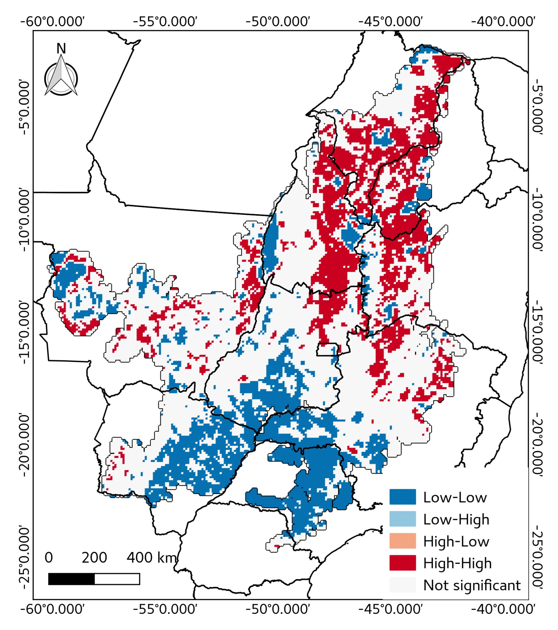
Local indicator of spatial autocorrelation (LISA) of LSS was explored by means of Local Moran’s (Equation (3) [61]). The LISA map is useful to understand the spatial patters of autocorrelation of the values of LSS, once it indicate clusters of low values with neighbours of low values (LL), high values with neighbours of high values (HH) and local high or low values with neighbours of low and high values (HL and LH, respectively), meaning a transition zones between LL and HH [62]. In the case of the LSS, the LISA map shows significant regions of land sharing (HH) or sparing (LL) patterns, which allows users to identify these patterns beyond the single cell to broader scales, as well as their spatial variation.
where, n is the number of attributes; is the attribute value in region i; is the attribute value in region j; is the mean value of the attribute in the study site; and are weights according to the neighbourhood of the attributes.
In general, there are global and local regression models. Whereas global models seek to investigate the average strenght and significance of statistical relationships between independent and dependent variables with just one equation for all data [63], local models detect spatial variation of relationships and produce maps for exploring and interpreting spatial non-stationarity [64]. So, the local model called Geographically Weighted Regression (GWR) was used for modelling the spatial relationship between LSS and rural population because it permits to explore the local relationships between the variables, providing a useful tool for finding relevant spots at the landscape scale. GWR is often used as descriptive and exploratory tool [65] and inferences cannot be done because the non-linear term cannot be added in the model [64,65].
The GWR model calculates an unique set of parametres for each observation, defined by geographic coordinates and considers neighbouring values due to spatial dependence, as shown in Equation (4) [66]. GWR estimates the parameters and errors for the cells according to their locations based on a distance matrix and a bandwidth, adaptively calculated in this study. This approach enables to detect the spatial variation of the regression parameters.
where, is dependent variable LSS; is the independent variable (population); is the Gaussian error in location i; (, ) is the x, y coordinate in the location; is the local intercept coefficient; and is the local angular coefficient.
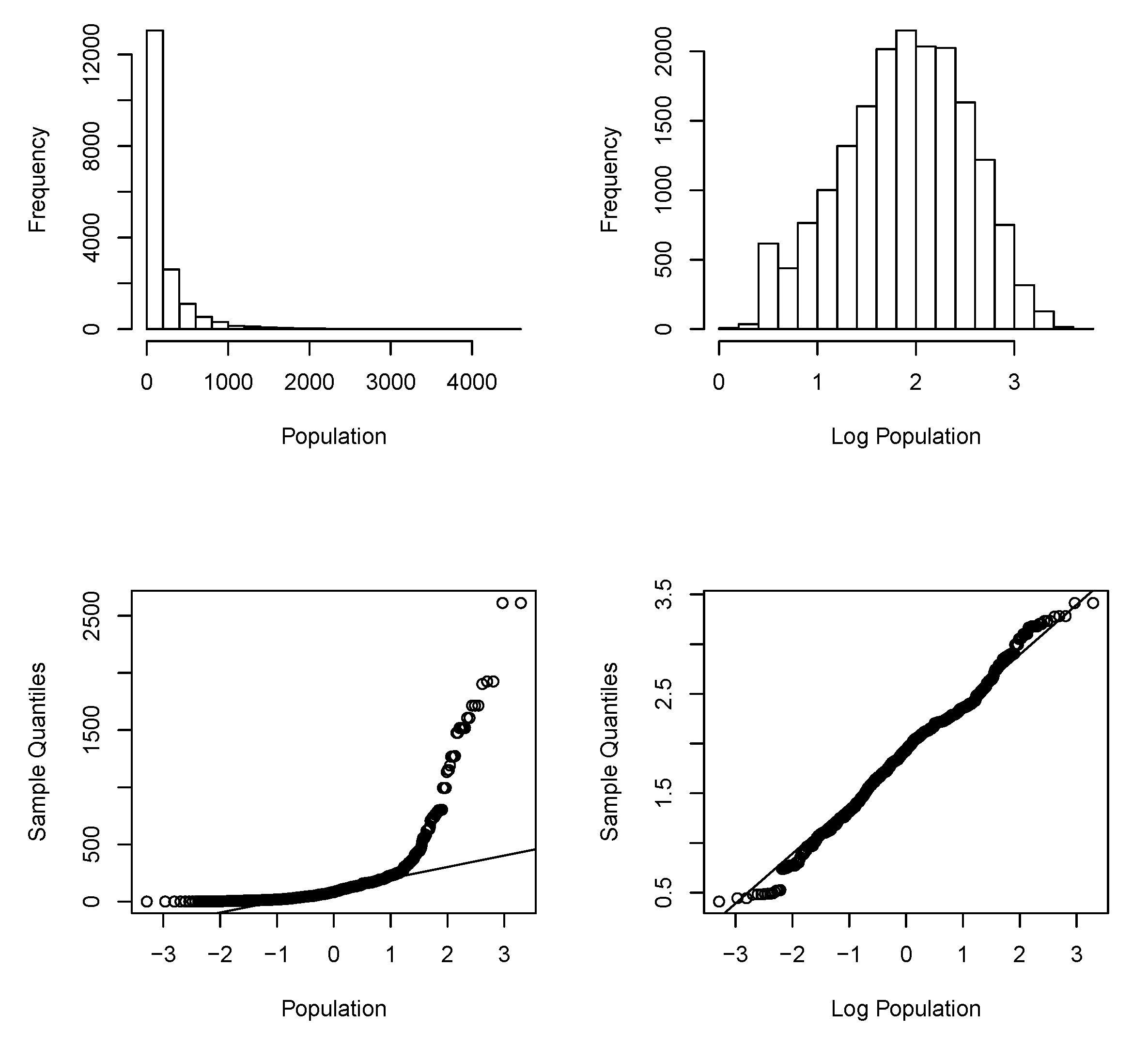
Before running GWR, the independent variable was evaluated for normality, both in its original and logarithmic form, a common transformation of the dependent variable to deal with possible non-normality [67]. Normality was evaluated by means of histogram and quantile-quantile (Q-Q) plot, following [68], where the logarithmic form was reasonably well represented by a normal distribution, as shown Figure 3.
All the methodological steps were conducted using open source software (R and QGIS) and open databases (IBGE and TerraClass), thus the steps are reproducible and easy to apply to other contexts.
3. Results
3.1. Land Sharing/Sparing Index
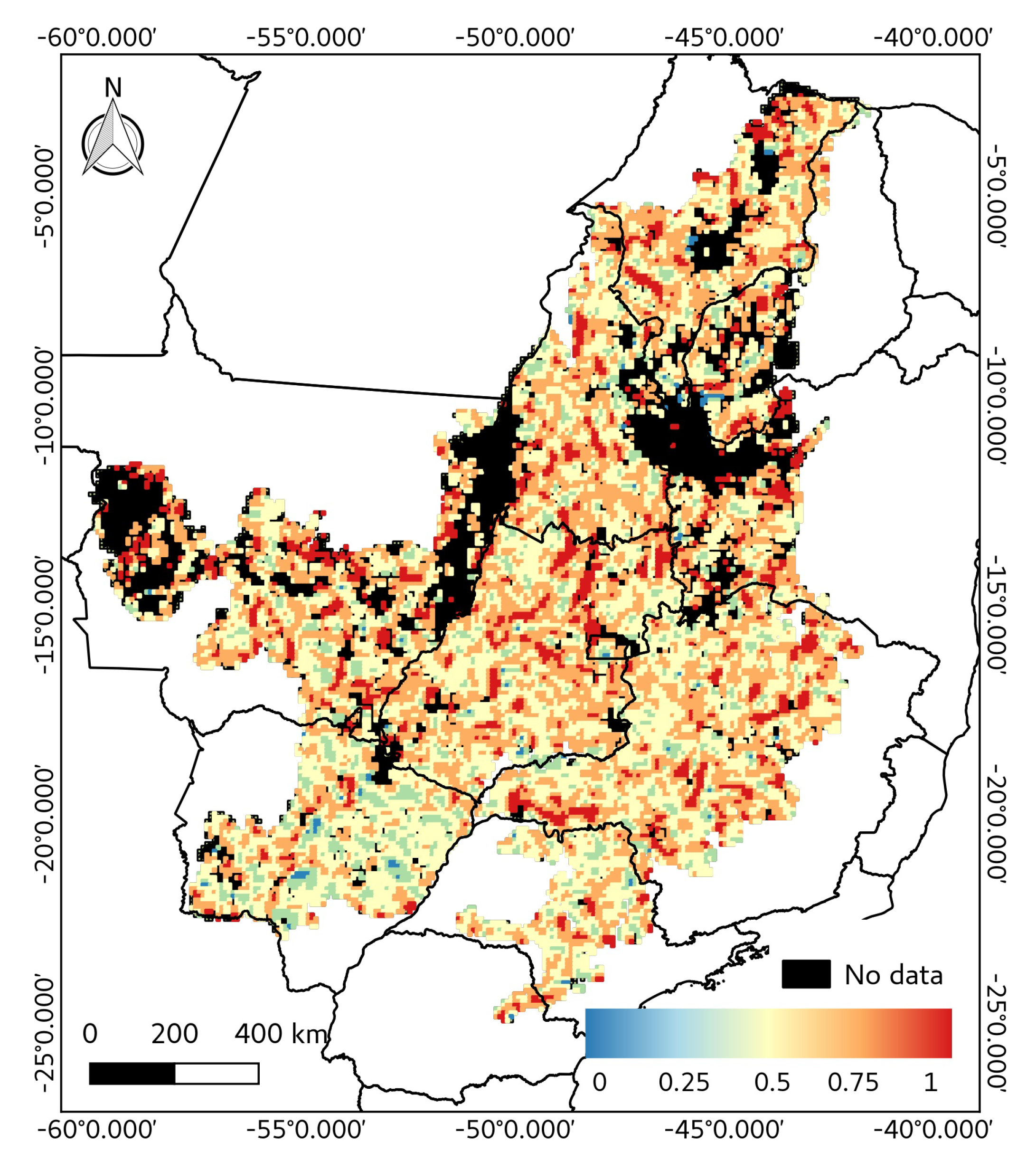
The gridded Land Sharing/Sparing Index (LSS) is shown in Figure 4. The global Moran’s I for LSS was 0.751, indicating positive global spatial autocorrelation of LSS values in the Cerrado.
Cells filled solely with natural land cover classes actually occupies only 6.4% of the Cerrado area. These areas are mainly protected by integral Conservation Units and Indigenous Lands and are the only remaining places suitable for sparing natural vegetation on contiguous patches larger or equal to 100 km. Cells whose proportion of natural areas accounts for less than 0.5 (50%) covers almost half of the Cerrado (48%), mainly located in the southern portion, where the anthropogenic occupation date back from the beginning of the 20th century [69].
There is a clear pattern of land sharing-dominated agricultural landscapes in the northern portion of Cerrado, while the opposite is found in the southern portion. This pattern is confirmed by the LISA map (Figure 5), where High-High clusters of LSS values (24% of the cells) predominate mainly in the north, while Low-Low clusters (28% of the cells) prevail in the south. No significant spatial autocorrelation of LSS (47% of the cells) was found mainly in the centre of the Cerrado. High-Low and Low-High transition clusters accounts for less than 1% of the region, which is in accordance to the rationale of the index’s endpoints, indicating the separation of the land sharing/sparing patterns in the region.
3.2. Rural Population Disaggregation
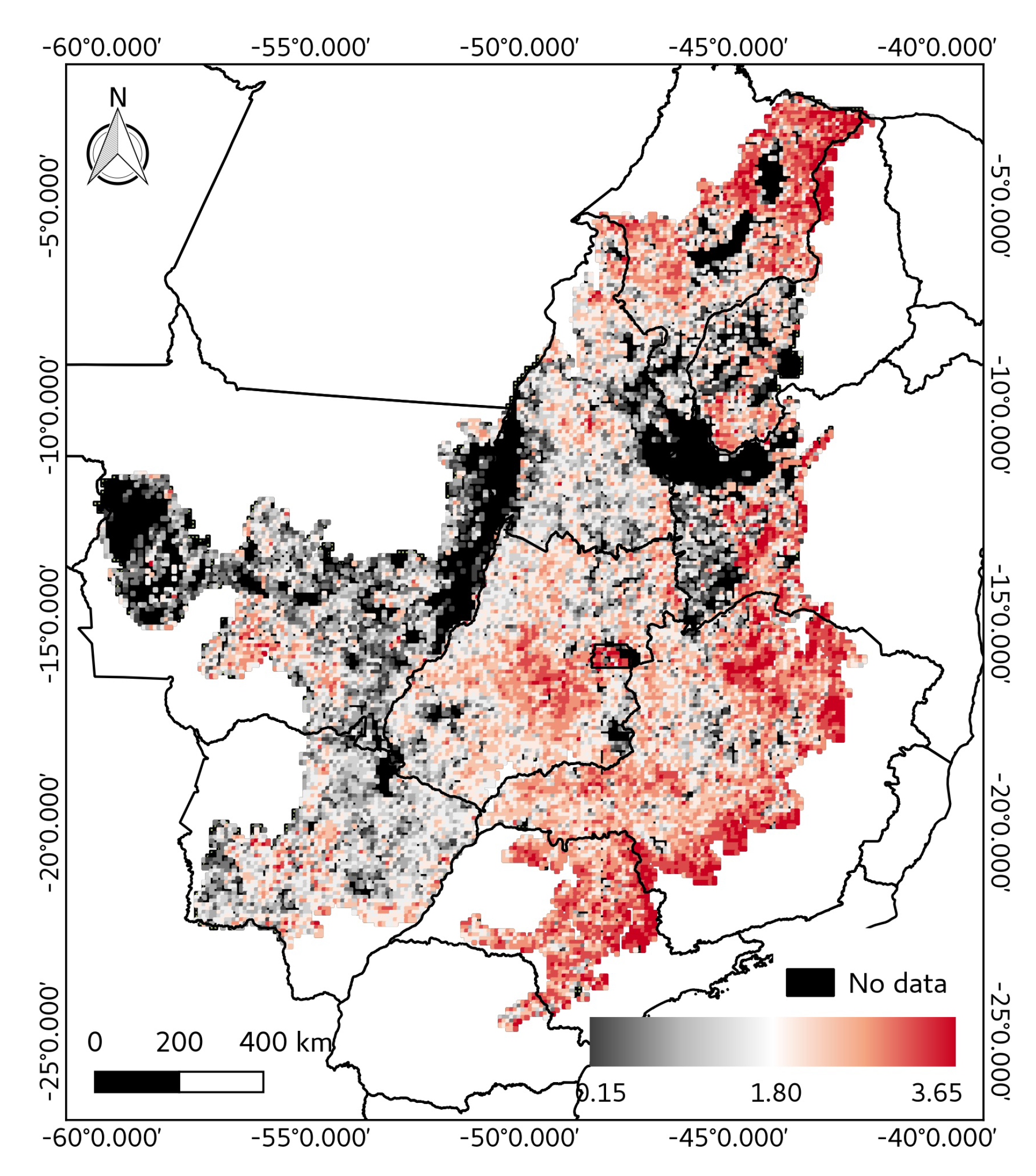
Rural population in the Cerrado is mainly clustered in the northern (Maranhão and Piauí states), southeaster (Bahia, Minas Gerais, São Paulo and Paraná states) and in central portions (Goiás’s capital Goiânia region and in the Federal District), as shown in logarithmic form in Figure 6 to facilitate visualization of population distribution.
The total estimated rural population accounted for 3,439,621 inhabitants.Even though, we would expect this result to be underestimated because of loss of household’s location data, it is still in agreement to previous analysis of the Cerrado’s population dynamics [70]. It evidences the method for integrating CNEFE’s households locations and data at the census tracts into grid cells is appropriated for the spatial disaggregation of the rural population in the Cerrado.
Cells with less than 100 people accounts for 55% of total cells, meaning a population density of less than one person per km. Alternatively, the most densely populated cells range from 10 to 44 inhabitants per km, which are only 2.5% of the cells. The mean population density is 1.9 inhabitants per km and standard deviation of 2.9 inh/km.
3.3. LSS and Rural Population
Globally, rural population density explained 87% (Quasi-global R 0.87) of Land Sharing/Sparing Index variation with the decreased AIC corrected (AICc) of 4291.177 and residual sum of squares = 658.3349. Moreover, the ANOVA comparison results also showed the GWR local model was significantly more appropriate than the OLS global model (F = 11.451, p < 0.001). It means that GWR was more suitable than the OLS.
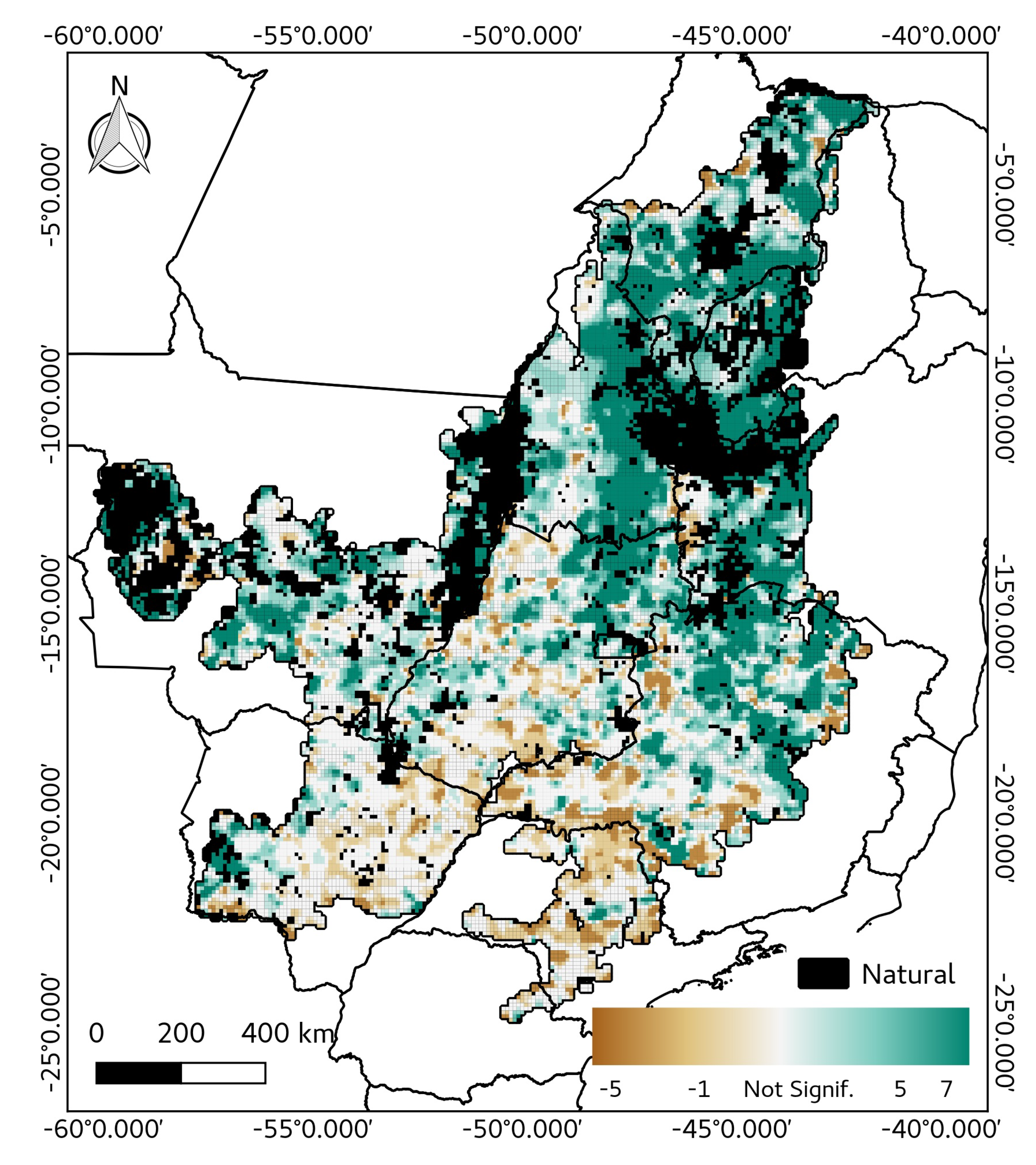
Figure 7 shows the slopes of the local regressions (angular coefficients ) of the Geographically Weighted Regression model. This parameter describes the magnitude and nature of the relationship between LSS and rural population density, meaning the rate of change in the LSS with an unit of change in the independent variable.
The map shows clusters of positive and negative relationship between rural population and LSS. The spatial variation of values evidences that the intensity of this relationship varies among different landscapes, where positive values are those regions that the hypothesis of the study is confirmed. Most of the coefficients are positive (68%), suggesting that in the Cerrado region, the higher the rural population density the higher is the LSS index. In these areas of positive association, the land sharing strategy is more suitable for managing the landscape, considering the social features of agriculture coupled with environmental conservation.
Negative significant values account for approximately 9% of Cerrado region, where an inverse relationship between LSS and rural population is found, i.e.,: the higher the population density the larger portions showing land sparing patterns in the landscape. A round quarter of Cerrado region did not present statistical significant association between rural population density and the LSS index proposed here.
Positive statistically significant relationships indicated by GWR are mainly concentrated in the northern portion of Minas Gerais and Goiás states, as well as in the centre-west of Mato Grosso and in the so-called MATOPIBA region (acronym for Maranhão, Tocantins, Piauí and Bahia states). This area with, specific strategic governance actions to support large scale agriculture, occupyies 32% of the Cerrado region into its northern part where land sharing patches are still high according to LISA map results. On the other hand, negative association between the variables are found in the southern portion Cerrado, where rural areas are relatively dense, but the predominant land sparing pattern is observed across the landscapes.
The local coefficients of determination (local R) of GWR spatially evidences the degree which the response variable was able to explain the local variations in the dependent variable, and the result is shown in Figure 8. The local R gives a measure of significance of the model. Overall, higher significance was found in the centre of the Cerrado region, but in general the model was well fitted, despite some minor areas with lower R in the north and in Mato Grosso do Sul, Minas Gerais and São Paulo states.
Finally, Figure 9 shows the standard error of the estimate (se(y)), which is a measure of the spread of the estimates around the fitted value and is helpful for investigating the precision of the spatial variation of the estimate [71]. As can be seen in the map, most of the local regressions have relative low se(y), indicating that the model is less precise in the borders of Minas Gerais state and in the centre of Goiás state.
4. Discussion
4.1. Spatial Analysis
The current approach makes two main important contributions to the land sharing/sparing debate. First, a high resolution spatial explicit indicator of patterns of land sharing/sparing was developed. The positive spatial autocorrelation of LSS index was expected in some regions, due to the fact that agricultural land use classes tend to be closer to higher accessible areas and routes of production flows. Thus, a learning point was the land sharing-dominated patterns in northern areas where large scale agriculture has expanded significantly in the last decade and it is expected to keep expanding in the near future [72,73,74]. In this sense, the shift towards a land sparing pattern in this specific region may have consequences on both human population and ecosystem services dynamics.
As a second contribution, the hypothesis of a positive relationship between rural population density and land sharing at landscape scales was corroborated by means of spatial analysis tools. The adopted method for integrating rural households locations and population data at the census tracts into grid cells showed meaningful results correlated to LSS indexes, and therefore was considered a successful method to spatially disaggregate rural from urban population in the Cerrado.
4.2. Land Sharing/Sparing in the Cerrado
According to [31], it is not clear whether land sparing or land sharing are conceptually tied to a particular landscape, therefore it is often ill-defined when sharing becomes sparing and a landscape may be considered as an example of land sparing for some and land sharing for others. In this study, the assumptions made considered that gridded landscapes of 100 km were suitable for studying spatial patterns of land sharing in a region with more than 2 million km, by means of an index based on a single year land use and land cover map. Recent spatio-temporal and multiscale spatial analysis tools currently under development and implementation, such as the Geographical and Temporal Weighted Regression (GTWR) [75] and the Multiscale Geographically Weighted Regression (MGWR) [76], offers future possibilities for addressing the temporal and multiscale issue of rural population densities and the land sharing and land sparing patterns of agriculture in Cerrado region.
The positive angular coefficients, resulted from spatial analysis, indicate the landscapes that are more likely to shape the land sharing pattern of integrating land use for agriculture and wildlife-friendly habitats, taking into account the social aspects for the conservation of natural environments. However, the higher values are located in the main agricultural expansion frontier for grains in Brazil, the MATOPIBA region [77]. In this sense, a spatio-temporal analysis of this territory is needed to monitor and to develop local policies for land use, as well as to access the impact of current land sharing on the biodiversity status of preservation.
In the land sharing scope, the agriculture is seen as an essential part of the biodiversity conservation agenda [43], so studies in other scales could enhance the understanding about the possible benefits and trade-offs of land sharing in the Brazilian Cerrado. The results are also meaningful because they highlighted that only about 6% of the Cerrado may still be unmanaged, considering vast areas of contiguous natural vegetation larger than 100 km, therefore, those are the only available lands for sparing. Even though this sparing strategy may have contributed to the maintenance of natural land cover in the past, the conservation benefits land sparing in the future is a matter of debate [78]. The central means to promote land sparing is by intensifying agriculture, however higher yields do not necessarily result in lower demand for new agricultural lands [79]. In this sense, there is no evidence of agricultural expansion slowdown in the Cerrado [80], especially in the MATOPIBA, where agricultural expansion is observed along with any yield improvements in the last decades [81], which reduces the amount of both natural areas and land suitable for sharing.
In such context, geopolitical strategies to promote land use systems based on the LSS model shall not focus only on increasing yields in land sparing dominated patterns, but also on regional decisions capable of keeping existing high indexes of land sharing associated to concentrated rural population. Regarding production aspects, the enhancement of multimodal accessibility and infrastructure networks capable to attend future domestic and international trading demands, represent a key factor that might jeopardize land sharing dominated landscapes [82]. Considering Brazilian historical autocorrelation between forest depletion and increased accessibility [83,84,85], smart policies based on land sparing vs. land sharing models must take into account the local potentialities of existing roads, railways or fluvial transportation. Thus regional conservation and agricultural production benefits can be obtained by policies that tackle both modernization of infrastructure (especially regarding terrestrial road routes of grain commodities from the south of Cerrado into south-eastern Brazil), and less impacting networks as railroads and especially fluvial transportation (meat and agricultural exports from northeast Cerrado into north and northeast Brazil). Last, but not least infrastructural planning must include participative governance of rural population, especially traditional communities and indigenous people, whose role in land sharing conservation patterns has been largely recognized [86].
Although it is not clear how large should natural habitats be spared for wildlife conservation and ecosystem self-maintenance [87], according to our scale of analysis, there are more suitable areas for a high quality matrix land sharing model of agriculture in the Cerrado than for sparing natural lands from agriculture (24% against 6%). Policies on land sharing strategies can reduce the threats on natural fragments, preserving important ecosystem services, and work positively on a sustainable landscape in Cerrado region, harmonizing the increase of agriculture yield and minimizing the impact of conservation areas.
5. Conclusions
In this research, the spatial relationships between local rural population and land sharing/sparing patterns were explored by means of GIS and spatial modelling. It was found that, in the scale of analysis, spatial clusters of land sharing are more likely to occur in northern portions of the Cerrado. Although there is a clustering trend within the rural population in eastern Cerrado, a positive association between land sharing and rural population were identified in some areas in the centre-north of the region.
The spatial index proposed in this study derived from land use maps is easy to apply to other contexts and environments and, associated with population data, indicates the potential areas for agriculture intensification and/or for supporting food production in biodiversity-friendly landscapes managed by local rural populations. So, this approach can be widely used by stakeholders to evaluate the status of agricultural landscapes.
In practice, the approach revealed that the amount of large natural environments available in the landscape for sparing nature from agriculture in the Cerrado is about only 6% of its total area, which means that agriculture expansion may be limited. Also, it suggests that in the centre-northern portion of the Cerrado there are possible areas where joint agricultural activities and social arrangements could be of high relevance for biodiversity conservation.
Thus, policymakers should support land sharing in these areas as an opportunity for the development of local initiatives for sustainable wildlife-friendly agriculture and maintenance of important ecosystem services in this region. Notwithstanding, closing yeld gaps in areas of intensive farming is needed to avoid expanssion, optimizing both strategies of land sharing and land sparing.
Finally, the major limitations of this research are on the common unavailability of high resolution and updated data of tropical landscapes, such as high resolution land use maps and population census, as well as the exploratory feature of GWR, which constrains its use as an inferential tool.
Author Contributions
João Pompeu conceived, analysed and wrote the paper; Luciana Soler wrote and reviewed the paper; Jean Ometto. supervised the project, wrote and reviewed the paper.
Funding
Fundação de Amparo à Pesquisa do Estado de São Paulo: 16/02773-5, Fundação de Amparo à Pesquisa do Estado de São Paulo: 2014/50627-2, PROEX/CAPES
Acknowledgments
We are grateful to Silvana Amaral and Miguel Monteiro for their useful contribution to this work. We also thank the Coordenação de Aperfeiçoamento de Pessoal de Nível Superior (CAPES) for the doctorate scholarship granted to the first author and to the Fundação de Amparo à Pesquisa do Estado de São Paulo (FAPESP), for the post-doctorate scholarship granted to the second author (process 16/02773-5) and for funding the “Delivering Food Security on Limited Land—DEVIL” project, in the scope of the Belmont Forum FACCE-JPI 2013 (process 2014/50627-2), which this research is part of. We also acknowledge the DEVIL project team, especially Pete Smith for his encouraging comments, as well as the anonymous reviewers that made valuable suggestions for improving this paper.
Conflicts of Interest
The authors declare no conflict of interest.
References
- Ellis, E.C.; Klein Goldewijk, K.; Siebert, S.; Lightman, D.; Ramankutty, N. Anthropogenic transformation of the biomes, 1700 to 2000. Glob. Ecol. Biogeogr. 2010, 19, 589–606. [Google Scholar] [CrossRef]
- Erb, K.H.; Luyssaert, S.; Meyfroidt, P.; Pongratz, J.; Don, A.; Kloster, S.; Kuemmerle, T.; Fetzel, T.; Fuchs, R.; Herold, M.; et al. Land management: Data availability and process understanding for global change studies. Glob. Chang. Biol. 2017, 23, 512–533. [Google Scholar] [CrossRef] [PubMed]
- Food and Agriculture Organization (FAO). State of the World’s Forests 2016. Forests and Agriculture: Land-Use Challenges and Opportunities; Food and Agriculture Organization: Rome, Italy, 2016. [Google Scholar]
- Ramankutty, N.; Mehrabi, Z.; Waha, K.; Jarvis, L.; Kremen, C.; Herrero, M.; Rieseberg, L.H. Trends in global agricultural land use: implications for environmental health and food security. Ann. Rev. Plant Biol. 2018, 69, 789–815. [Google Scholar] [CrossRef] [PubMed]
- Ceballos, G.; Ehrlich, P.R.; Barnosky, A.D.; García, A.; Pringle, R.M.; Palmer, T.M. Accelerated modern human–induced species losses: Entering the sixth mass extinction. Sci. Adv. 2015, 1, e1400253. [Google Scholar] [CrossRef] [PubMed] [Green Version]
- Smith, P.; Bustamante, M.; Ahammad, H.; Clark, H.; Dong, H.; Elsiddig, E.A.; Haberl, H.; Harper, R.; House, J.; Jafari, M.; et al. Agriculture, Forestry and Other Land Use (AFOLU). In Climate Change 2014: Mitigation of Climate Change. Contribution of Working Group Iii to the Fifth Assessment Report of the Intergovernmental Panel on Climate Change; Cambridge University Press: Cambridge, UK, 2014. [Google Scholar]
- Stehle, S.; Schulz, R. Agricultural insecticides threaten surface waters at the global scale. Proc. Natl. Acad. Sci. USA 2015, 112, 5750–5755. [Google Scholar] [CrossRef] [PubMed] [Green Version]
- Walker, L.; Wu, S. Pollinators and pesticides. In International Farm Animal, Wildlife and Food Safety Law; Springer: Berlin, Germany, 2017; pp. 495–513. [Google Scholar]
- Bombardi, L.M. Geography of the Use of Agrochemicals in Brazil and Connections with the European Union; FFLCH–USP: São Paulo, Brazil, 2017. [Google Scholar]
- Popp, J.; Kot, S.; Lakner, Z.; Oláh, J. Biofuel use: Peculiarities and Implications. J. Secur. Sustain. Issues 2018, 7, 3. [Google Scholar] [CrossRef]
- Langeveld, J.W.; Dixon, J.; van Keulen, H.; Quist-Wessel, P.F. Analyzing the effect of biofuel expansion on land use in major producing countries: evidence of increased multiple cropping. Biofuels Bioprod. Biorefining 2014, 8, 49–58. [Google Scholar] [CrossRef]
- Popp, J.; Lakner, Z.; Harangi-Rakos, M.; Fari, M. The effect of bioenergy expansion: Food, energy, and environment. Renew. Sustain. Energy Rev. 2014, 32, 559–578. [Google Scholar] [CrossRef]
- Garnett, T.; Appleby, M.; Balmford, A.; Bateman, I.; Benton, T.; Bloomer, P.; Burlingame, B.; Dawkins, M.; Dolan, L.; Fraser, D.; et al. Sustainable intensification in agriculture: Premises and policies. Science 2013, 341, 33–34. [Google Scholar] [CrossRef] [PubMed] [Green Version]
- Smith, P. Delivering food security without increasing pressure on land. Glob. Food Secur. 2013, 2, 18–23. [Google Scholar] [CrossRef]
- Kremen, C. Reframing the land-sparing/land-sharing debate for biodiversity conservation. Ann. N. Y. Acad. Sci. 2015, 1355, 52–76. [Google Scholar] [CrossRef] [PubMed] [Green Version]
- Phalan, B.; Balmford, A.; Green, R.E.; Scharlemann, J.P. Minimising the harm to biodiversity of producing more food globally. Food Policy 2011, 36, S62–S71. [Google Scholar] [CrossRef]
- Altieri, M.A. The ecological role of biodiversity in agroecosystems. Agric. Ecosyst. Environ. 1999, 74, 19–31. [Google Scholar] [CrossRef] [Green Version]
- Vandermeer, J.; Perfecto, I. The agricultural matrix and a future paradigm for conservation. Conserv. Biol. 2007, 21, 274–277. [Google Scholar] [CrossRef] [PubMed]
- Geiger, F.; Bengtsson, J.; Berendse, F.; Weisser, W.W.; Emmerson, M.; Morales, M.B.; Ceryngier, P.; Liira, J.; Tscharntke, T.; Winqvist, C.; et al. Persistent negative effects of pesticides on biodiversity and biological control potential on European farmland. Basic Appl. Ecol. 2010, 11, 97–105. [Google Scholar] [CrossRef]
- Winqvist, C.; Ahnström, J.; Bengtsson, J. Effects of organic farming on biodiversity and ecosystem services: Taking landscape complexity into account. Ann. N. Y. Acad. Sci. 2012, 1249, 191–203. [Google Scholar] [CrossRef] [PubMed]
- Balmford, A.; Green, R.; Scharlemann, J.P. Sparing land for nature: Exploring the potential impact of changes in agricultural yield on the area needed for crop production. Glob. Chang. Biol. 2005, 11, 1594–1605. [Google Scholar] [CrossRef]
- Green, R.E.; Cornell, S.J.; Scharlemann, J.P.; Balmford, A. Farming and the fate of wild nature. Science 2005, 307, 550–555. [Google Scholar] [CrossRef] [PubMed]
- Clough, Y.; Barkmann, J.; Juhrbandt, J.; Kessler, M.; Wanger, T.C.; Anshary, A.; Buchori, D.; Cicuzza, D.; Darras, K.; Putra, D.D.; et al. Combining high biodiversity with high yields in tropical agroforests. Proc. Natl. Acad. Sci. USA 2011, 108, 8311–8316. [Google Scholar] [CrossRef] [PubMed] [Green Version]
- Phalan, B.; Onial, M.; Balmford, A.; Green, R.E. Reconciling food production and biodiversity conservation: Land sharing and land sparing compared. Science 2011, 333, 1289–1291. [Google Scholar] [CrossRef] [PubMed]
- Fischer, J.; Batáry, P.; Bawa, K.S.; Brussaard, L.; Chappell, M.J.; Clough, Y.; Daily, G.C.; Dorrough, J.; Hartel, T.; Jackson, L.E.; et al. Conservation: Limits of land sparing. Science 2011, 334, 593. [Google Scholar] [CrossRef] [PubMed]
- Tscharntke, T.; Clough, Y.; Wanger, T.C.; Jackson, L.; Motzke, I.; Perfecto, I.; Vandermeer, J.; Whitbread, A. Global food security, biodiversity conservation and the future of agricultural intensification. Biol. Conserv. 2012, 151, 53–59. [Google Scholar] [CrossRef]
- Chandler, R.B.; King, D.I.; Raudales, R.; Trubey, R.; Chandler, C.; Arce Chávez, V.J. A Small-Scale Land-Sparing Approach to Conserving Biological Diversity in Tropical Agricultural Landscapes. Conserv. Biol. 2013, 27, 785–795. [Google Scholar] [CrossRef] [PubMed]
- Gabriel, D.; Sait, S.M.; Kunin, W.E.; Benton, T.G. Food production vs. biodiversity: Comparing organic and conventional agriculture. J. Appl. Ecol. 2013, 50, 355–364. [Google Scholar] [CrossRef]
- Mendenhall, C.D.; Archer, H.M.; Brenes, F.O.; Sekercioglu, C.H.; Sehgal, R.N. Balancing biodiversity with agriculture: Land sharing mitigates avian malaria prevalence. Conserv. Lett. 2013, 6, 125–131. [Google Scholar] [CrossRef] [Green Version]
- Von Wehrden, H.; Abson, D.J.; Beckmann, M.; Cord, A.F.; Klotz, S.; Seppelt, R. Realigning the land-sharing/land-sparing debate to match conservation needs: Considering diversity scales and land-use history. Landsc. Ecol. 2014, 29, 941–948. [Google Scholar] [CrossRef]
- Fischer, J.; Abson, D.J.; Butsic, V.; Chappell, M.J.; Ekroos, J.; Hanspach, J.; Kuemmerle, T.; Smith, H.G.; Wehrden, H. Land sparing versus land sharing: Moving forward. Conserv. Lett. 2014, 7, 149–157. [Google Scholar] [CrossRef]
- Gonthier, D.J.; Ennis, K.K.; Farinas, S.; Hsieh, H.Y.; Iverson, A.L.; Batáry, P.; Rudolphi, J.; Tscharntke, T.; Cardinale, B.J.; Perfecto, I. Biodiversity conservation in agriculture requires a multi-scale approach. Proc. R. Soc. Lond. B Biol. Sci. 2014, 281, 20141358. [Google Scholar] [CrossRef] [PubMed]
- Hodgson, J.A.; Kunin, W.E.; Thomas, C.D.; Benton, T.G.; Gabriel, D. Comparing organic farming and land sparing: Optimizing yield and butterfly populations at a landscape scale. Ecol. Lett. 2010, 13, 1358–1367. [Google Scholar] [CrossRef] [PubMed]
- Fischer, J.; Brosi, B.; Daily, G.C.; Ehrlich, P.R.; Goldman, R.; Goldstein, J.; Lindenmayer, D.B.; Manning, A.D.; Mooney, H.A.; Pejchar, L.; et al. Should agricultural policies encourage land sparing or wildlife-friendly farming? Front. Ecol. Environ. 2008, 6, 380–385. [Google Scholar] [CrossRef]
- Luskin, M.S.; Lee, J.S.; Edwards, D.P.; Gibson, L.; Potts, M.D. Study context shapes recommendations of land-sparing and sharing; A quantitative review. Glob. Food Secur. 2017, 16, 29–35. [Google Scholar] [CrossRef]
- Jiang, G.; Wang, G.; Holyoak, M.; Yu, Q.; Jia, X.; Guan, Y.; Bao, H.; Hua, Y.; Zhang, M.; Ma, J. Land sharing and land sparing reveal social and ecological synergy in big cat conservation. Biol. Conserv. 2017, 211, 142–149. [Google Scholar] [CrossRef]
- Edwards, D.P.; Gilroy, J.J.; Woodcock, P.; Edwards, F.A.; Larsen, T.H.; Andrews, D.J.; Derhé, M.A.; Docherty, T.D.; Hsu, W.W.; Mitchell, S.L.; et al. Land-sharing versus land-sparing logging: Reconciling timber extraction with biodiversity conservation. Glob. Chang. Biol. 2014, 20, 183–191. [Google Scholar] [CrossRef] [PubMed]
- Pywell, R.F.; Heard, M.S.; Woodcock, B.A.; Hinsley, S.; Ridding, L.; Nowakowski, M.; Bullock, J.M. Wildlife-friendly farming increases crop yield: Evidence for ecological intensification. Proc. R. Soc. B 2015, 282, 20151740. [Google Scholar] [CrossRef] [PubMed]
- Miller, J.R. Biodiversity conservation and the extinction of experience. Trends Ecol. Evol. 2005, 20, 430–434. [Google Scholar] [CrossRef] [PubMed]
- Folke, C.; Jansson, Å.; Rockström, J.; Olsson, P.; Carpenter, S.R.; Chapin, F.S., III; Crépin, A.S.; Daily, G.; Danell, K.; Ebbesson, J.; et al. Reconnecting to the biosphere. Ambio 2011, 40, 719–738. [Google Scholar] [CrossRef] [PubMed]
- Aide, T.M.; Grau, H.R. Globalization, migration, and Latin American ecosystems. Science 2004, 305, 1915–1916. [Google Scholar] [CrossRef] [PubMed]
- Wright, S.J.; Muller-Landau, H.C. The future of tropical forest species1. Biotropica 2006, 38, 287–301. [Google Scholar] [CrossRef]
- Perfecto, I.; Vandermeer, J. The agroecological matrix as alternative to the land-sparing/agriculture intensification model. Proc. Natl. Acad. Sci. USA 2010, 107, 5786–5791. [Google Scholar] [CrossRef] [PubMed] [Green Version]
- Figueiredo, A.A. Food production and the food industry in Brazil: Their impact on nutritional status. Food Rev. Int. 1989, 5, 237–250. [Google Scholar] [CrossRef]
- Ruel, M.T.; Garrett, J.; Yosef, S.; Olivier, M. Urbanization, food security and nutrition. In Nutrition and Health in a Developing World; Springer: Berlin. Germany, 2017; pp. 705–735. [Google Scholar]
- Vandermeer, J.; van Noordwijk, M.; Anderson, J.; Ong, C.; Perfecto, I. Global change and multi-species agroecosystems: Concepts and issues. Agric. Ecosyst. Environ. 1998, 67, 1–22. [Google Scholar] [CrossRef]
- Altieri, M.A.; Funes-Monzote, F.R.; Petersen, P. Agroecologically efficient agricultural systems for smallholder farmers: Contributions to food sovereignty. Agron. Sustain. Dev. 2012, 32, 1–13. [Google Scholar] [CrossRef]
- Garibaldi, L.A.; Gemmill-Herren, B.; D?Annolfo, R.; Graeub, B.E.; Cunningham, S.A.; Breeze, T.D. Farming approaches for greater biodiversity, livelihoods, and food security. Trends Ecol. Evol. 2017, 32, 68–80. [Google Scholar] [CrossRef] [PubMed]
- Berkes, F. Rethinking community-based conservation. Conserv. Biol. 2004, 18, 621–630. [Google Scholar] [CrossRef]
- Tscharntke, T.; Klein, A.M.; Kruess, A.; Steffan-Dewenter, I.; Thies, C. Landscape perspectives on agricultural intensification and biodiversity–ecosystem service management. Ecol. Lett. 2005, 8, 857–874. [Google Scholar] [CrossRef]
- Lin, B.B. Resilience in agriculture through crop diversification: adaptive management for environmental change. BioScience 2011, 61, 183–193. [Google Scholar] [CrossRef]
- Larsen, A.E.; Gaines, S.D.; Deschênes, O. Spatiotemporal variation in the relationship between landscape simplification and insecticide use. Ecol. Appl. 2015, 25, 1976–1983. [Google Scholar] [CrossRef] [PubMed]
- Chappell, M.J.; LaValle, L.A. Food security and biodiversity: Can we have both? An agroecological analysis. Agric. Human Values 2011, 28, 3–26. [Google Scholar] [CrossRef]
- Lahsen, M.; Bustamante, M.M.; Dalla-Nora, E.L. Undervaluing and overexploiting the Brazilian Cerrado at our peril. Environ. Sci. Policy Sustain. Dev. 2016, 58, 4–15. [Google Scholar] [CrossRef]
- Myers, N.; Mittermeier, R.A.; Mittermeier, C.G.; Da Fonseca, G.A.; Kent, J. Biodiversity hotspots for conservation priorities. Nature 2000, 403, 853–858. [Google Scholar] [CrossRef] [PubMed]
- Ministério do Meio Ambiente. Mapeamento do Uso e Cobertura do Cerrado: Projeto Terra Class Cerrado; Ministério do Meio Ambiente: Brasília, Brazil, 2015. [Google Scholar]
- Ganem, R.S.; Drummond, J.A.; Franco, J.L.d.A. Conservation polices and control of habitat fragmentation in the Brazilian Cerrado biome. Ambient. Soc. 2013, 16, 99–118. [Google Scholar] [CrossRef]
- De Oliveira D’Antona, Á.; Bueno, M.d.C.D.; de Sampaio Dagnino, R. Estimativa da população em unidades de conservação na Amazônia Legal brasileira–uma aplicação de grades regulares a partir da Contagem 2007. Rev. Bras. Estud. Pop. 2013, 30, 401–428. [Google Scholar]
- Amaral, S.; Gavlak, A.A.; Escada, M.I.S.; Monteiro, A.M.V. Using remote sensing and census tract data to improve representation of population spatial distribution: Case studies in the Brazilian Amazon. Popul. Environ. 2012, 34, 142–170. [Google Scholar] [CrossRef]
- Tammisto, R. Merging national population grids (bottom-up approach) into a European dataset. In GIS for Statistics; Anais: Luxembourg, 2007. [Google Scholar]
- Smith, M.J.; Goodchild, M.F.; Longley, P. Geospatial Analysis: A Comprehensive Guide to Principles, Techniques and Software Tools; Troubador Publishing Ltd.: Leicester, UK, 2007. [Google Scholar]
- Anselin, L. Local indicators of spatial association—LISA. Geogr. Anal. 1995, 27, 93–115. [Google Scholar] [CrossRef]
- Gilbert, A.; Chakraborty, J. Using geographically weighted regression for environmental justice analysis: Cumulative cancer risks from air toxics in Florida. Soc. Sci. Res. 2011, 40, 273–286. [Google Scholar] [CrossRef]
- Fotheringham, A.S.; Brunsdon, C.; Charlton, M. Geographically Weighted Regression; John Wiley & Sons Ltd.: West Atrium, Canada, 2003. [Google Scholar]
- Finley, A.O. Comparing spatially-varying coefficients models for analysis of ecological data with non-stationary and anisotropic residual dependence. Methods Ecol. Evol. 2011, 2, 143–154. [Google Scholar] [CrossRef]
- Brunsdon, C.; Fotheringham, A.; Charlton, M. Geographically weighted summary statistics: A framework for localised exploratory data analysis. Comput. Environ. Urban Syst. 2002, 26, 501–524. [Google Scholar] [CrossRef]
- Faraway, J.J. Practical Regression and ANOVA Using R. 2002. Available online: http://cran.r-project.org/doc/contrib/Faraway-PRA.pdf (accessed on 20 July 2018).
- Benitez, F.L.; Anderson, L.O.; Formaggio, A.R. Evaluation of geostatistical techniques to estimate the spatial distribution of aboveground biomass in the Amazon rainforest using high-resolution remote sensing data. Acta Amazon. 2016, 46, 151–160. [Google Scholar] [CrossRef] [Green Version]
- Klink, C.A.; Moreira, A.G. Past and current human occupation, and land use. Cerrados Braz. Ecol. Natl. Hist. Neot. Savanna 2002, 5, 69–90. [Google Scholar]
- Ojima, R.; Martine, G. Resgates sobre População e Ambiente: Breve análise da Dinâmica Demográfica e a Urbanização nos Biomas Brasileiros. Idéias 2012, 3, 5. [Google Scholar] [CrossRef]
- Brunsdon, C.; Fotheringham, S.; Charlton, M. Geographically weighted regression. J. R. Stat. Soc. Ser. D 1998, 47, 431–443. [Google Scholar] [CrossRef]
- Spera, S.A.; Galford, G.L.; Coe, M.T.; Macedo, M.N.; Mustard, J.F. Land-use change affects water recycling in Brazil’s last agricultural frontier. Glob. Chang. Biol. 2016, 22, 3405–3413. [Google Scholar] [CrossRef] [PubMed]
- Aguiar, A.S. Modelagem da DinÂmica do Desmatamento Na RegiÃo do MATOPIBA Até 2050. Master’s Dissertation, Universidade de Brasilia (UNB), Brasilia, Brazil, 2016. [Google Scholar]
- Silva, R.F.B.d.; Batistella, M.; Dou, Y.; Moran, E.; Torres, S.M.; Liu, J. The Sino-Brazilian telecoupled soybean system and cascading effects for the exporting country. Land 2017, 6, 53. [Google Scholar] [CrossRef]
- Fotheringham, A.S.; Crespo, R.; Yao, J. Geographical and temporal weighted regression (GTWR). Geogr. Anal. 2015, 47, 431–452. [Google Scholar] [CrossRef]
- Fotheringham, A.S.; Yang, W.; Kang, W. Multiscale Geographically Weighted Regression (MGWR). Ann. Am. Assoc. Geogr. 2017, 107, 1247–1265. [Google Scholar] [CrossRef]
- Silva, A.J.; do Socorro Lira Monteiro, M.; Barbosa, E.L. New productive dynamics and old territorial issues in the northern cerrados from Brazil. Espacios 2015, 36, 14–22. [Google Scholar]
- Ewers, R.M.; Scharlemann, J.P.; Balmford, A.; Green, R.E. Do increases in agricultural yield spare land for nature? Glob. Chang. Biol. 2009, 15, 1716–1726. [Google Scholar] [CrossRef] [Green Version]
- Rudel, T.K.; Schneider, L.; Uriarte, M.; Turner, B.L.; DeFries, R.; Lawrence, D.; Geoghegan, J.; Hecht, S.; Ickowitz, A.; Lambin, E.F.; et al. Agricultural intensification and changes in cultivated areas, 1970–2005. Proc. Natl. Acad. Sci. USA 2009, 106, 20675–20680. [Google Scholar] [CrossRef] [PubMed]
- Lapola, D.M.; Martinelli, L.A.; Peres, C.A.; Ometto, J.P.; Ferreira, M.E.; Nobre, C.A.; Aguiar, A.P.D.; Bustamante, M.M.; Cardoso, M.F.; Costa, M.H.; et al. Pervasive transition of the Brazilian land-use system. Nat. Clim. Chang. 2014, 4, 27–35. [Google Scholar] [CrossRef]
- Dias, L.C.; Pimenta, F.M.; Santos, A.B.; Costa, M.H.; Ladle, R.J. Patterns of land use, extensification, and intensification of Brazilian agriculture. Glob. Chang. Biol. 2016, 22, 2887–2903. [Google Scholar] [CrossRef] [PubMed]
- Strassburg, B.B.; Brooks, T.; Feltran-Barbieri, R.; Iribarrem, A.; Crouzeilles, R.; Loyola, R.; Latawiec, A.E.; Oliveira Filho, F.J.; Scaramuzza, C.A.d.M.; Scarano, F.R.; et al. Moment of truth for the Cerrado hotspot. Nat. Ecol. Evol. 2017, 1, 0099. [Google Scholar] [CrossRef] [PubMed]
- Soares-Filho, B.; Alencar, A.; Nepstad, D.; Cerqueira, G.; Diaz, V.; del Carmen, M.; Rivero, S.; Solorzano, L.; Voll, E. Simulating the response of land-cover changes to road paving and governance along a major Amazon highway: the Santarém–Cuiabá corridor. Glob. Chang. Biol. 2004, 10, 745–764. [Google Scholar] [CrossRef]
- Alves, D.S. Space-time dynamics of deforestation in Brazilian Amazonia. Int. J. Remote Sens. 2002, 23, 2903–2908. [Google Scholar] [CrossRef]
- Jusys, T. Fundamental causes and spatial heterogeneity of deforestation in Legal Amazon. Appl. Geogr. 2016, 75, 188–199. [Google Scholar] [CrossRef]
- Brondizio, E.S.; Le Tourneau, F.M. Environmental governance for all. Science 2016, 352, 1272–1273. [Google Scholar] [CrossRef] [PubMed]
- Stephens, P.A. Land sparing, land sharing, and the fate of Africa?s lions. Proc. Natl. Acad. Sci. USA 2015, 112, 14753–14754. [Google Scholar] [CrossRef] [PubMed] [Green Version]
Figure 1.
Relative location and 2013 land use and land cover map of the Cerrado [56]. Acronyms for Brazilian states stand for: Bahia (BA), Distrito Federal (DF), Goiás (GO) Maranhão (MA), Minas Gerais (MG), Mato Grosso do Sul (MS), Mato Grosso (MT), Paraná (PR), São Paulo (SP) and Tocantins (TO).
Figure 1.
Relative location and 2013 land use and land cover map of the Cerrado [56]. Acronyms for Brazilian states stand for: Bahia (BA), Distrito Federal (DF), Goiás (GO) Maranhão (MA), Minas Gerais (MG), Mato Grosso do Sul (MS), Mato Grosso (MT), Paraná (PR), São Paulo (SP) and Tocantins (TO).

Figure 2.
Flowchart illustrating the steps for spatial disaggregation of rural population in the Cerrado, based on Census tracts and household location. Data: 2010 Population Census and CNEFE.
Figure 2.
Flowchart illustrating the steps for spatial disaggregation of rural population in the Cerrado, based on Census tracts and household location. Data: 2010 Population Census and CNEFE.

Figure 3.
Histograms are shown in the top and Q-Q plots with normality line in the bottom. In the left the original data is presented and in the right the logarithmic form is presented.
Figure 3.
Histograms are shown in the top and Q-Q plots with normality line in the bottom. In the left the original data is presented and in the right the logarithmic form is presented.

Figure 4.
Gridded Land Sharing/Sparing Index for the Cerrado. Negative values (red) indicates more land sparing-oriented landscape and positive values (green) indicates more land sharing-oriented landscapes.
Figure 4.
Gridded Land Sharing/Sparing Index for the Cerrado. Negative values (red) indicates more land sparing-oriented landscape and positive values (green) indicates more land sharing-oriented landscapes.
Figure 5.
LISA map for LSS. Red patches indicates the predominance of agricultural landscapes more oriented to a land sharing pattern, while blue patches indicates land sparing pattern predominance in the landscape.
Figure 5.
LISA map for LSS. Red patches indicates the predominance of agricultural landscapes more oriented to a land sharing pattern, while blue patches indicates land sparing pattern predominance in the landscape.

Figure 6.
Logarithmic map of rural population density in the Cerrado based on CENEFE and Census tracts.
Figure 6.
Logarithmic map of rural population density in the Cerrado based on CENEFE and Census tracts.

Figure 7.
Local angular coefficients () of GWR model for rural population density.

Figure 8.
Local coefficients of determination (local R).

Figure 9.
Standard error of the logarithmic form of rural population.

Table 1.
Area of each land use and land cover classes in the Cerrado [56].
Table 1.
Area of each land use and land cover classes in the Cerrado [56].
| Class | Area (km) | % | |
|---|---|---|---|
| Anthropogenic land use | Permanent crops * | 174,006 | 8.53 |
| Temporary crops * | 64,512 | 3.16 | |
| Mining | 247 | 0.01 | |
| Occupation mosaic | 2326 | 0.11 | |
| Pasture * | 600,832 | 29.46 | |
| Silviculture * | 30,525 | 1.50 | |
| Bare soil | 3621 | 0.18 | |
| Urban area | 8797 | 0.43 | |
| Other | 73 | 0.00 | |
| Total anthropogenic | 884,939 | 43.38 | |
| Natural | Forest | 418,789 | 20.54 |
| Non-forest | 692,301 | 33.95 | |
| Non-vegetated | 2609 | 0.13 | |
| Total natural | 1,113,699 | 54.62 | |
| Water bodies | 15,056 | 0.74 | |
| Not observed | 25,549 | 1.25 | |
| Total | 2,039,243 | 100 |
* Anthropogenic classes merged for LSS.
© 2018 by the authors. Licensee MDPI, Basel, Switzerland. This article is an open access article distributed under the terms and conditions of the Creative Commons Attribution (CC BY) license (http://creativecommons.org/licenses/by/4.0/).
Share and Cite
MDPI and ACS Style
Pompeu, J.; Soler, L.; Ometto, J. Modelling Land Sharing and Land Sparing Relationship with Rural Population in the Cerrado. Land 2018, 7, 88. https://doi.org/10.3390/land7030088
AMA Style
Pompeu J, Soler L, Ometto J. Modelling Land Sharing and Land Sparing Relationship with Rural Population in the Cerrado. Land. 2018; 7(3):88. https://doi.org/10.3390/land7030088
Chicago/Turabian StylePompeu, João, Luciana Soler, and Jean Ometto. 2018. "Modelling Land Sharing and Land Sparing Relationship with Rural Population in the Cerrado" Land 7, no. 3: 88. https://doi.org/10.3390/land7030088
Note that from the first issue of 2016, this journal uses article numbers instead of page numbers. See further details here.