Article

Modelling Farm Growth and Its Impact on Agricultural Land Use: A Country Scale Application of an Agent-Based Model

by
Veronique Beckers
1,2,*,
Jeroen Beckers
3,
Matthias Vanmaercke
4,
Etienne Van Hecke
2,
Anton Van Rompaey
2 and
Nicolas Dendoncker
1
1
Department of Geography, UNamur, rue de Bruxelles 61, 5000 Namur, Belgium
2
Geography and Tourism Research Group, Department Earth and Environmental Science, KU Leuven, Celestijnenlaan 200E, 3001 Heverlee, Belgium
3
NVISO, Sinter-Goedelevoorplein 5 Parvis Sainte-Gudule, 1000 Brussels, Belgium
4
Département de Géography, Université de Liège, Quartier Village 4, Clos Mercator 3—B11, 4000 Liège, Belgium
*
Author to whom correspondence should be addressed.
Land 2018, 7(3), 109; https://doi.org/10.3390/land7030109
Submission received: 23 August 2018 / Revised: 9 September 2018 / Accepted: 13 September 2018 / Published: 15 September 2018

Abstract

:
The ongoing economic pressure on farmers has resulted in lower gross margins, lower income, and a continuous decrease in the number of farmers in large parts of the world. Most remaining farmers upscale their activities by taking over the land of their former competitors, resulting in a decrease in agricultural employment and an increase in average farm size, accompanied by specialisation and new management techniques. Understanding these significant trends and their impact on the land use and environment requires a deeper knowledge of the mechanisms involved and the impacts of different policy measures. These processes are ideally represented through agent-based modelling. Currently, agent-based models are rarely for larger regions. This paper presents ADAM (Agricultural Dynamics through Agent-based Modelling), using it for the case study of Belgium. ADAM was created to obtain insights in past and current agricultural trends and to explore possible effects of policy measures. ADAM simulates the evolution of a farmer population and their farms at a fine scale on the country level. It produces yearly outputs on the number of farms, their size, and the type of farming activity on every parcel. Results show that ADAM is capable of adequately modelling a farmer population according to past trends and that it can be used to explore the results of a business-as-usual scenario, therefore showing the possibility of creating agent-based models for larger scale real-world applications.

1. Introduction

The ongoing industrialisation of agriculture together with the recent globalisation of agricultural markets puts pressure on the profitability of farming activities in countries with an above-average population density [1]. The increasing competition among farmers has resulted in a decrease in the number of farmers. Often, small and uncompetitive farmers are either forced to end their activities or do not find a successor after retirement [2]. This may allow the remaining farmers to upscale their activities by taking over the land of their former competitors. This process is often accompanied by specialisation and a change in agricultural management [2,3], allowing investments in specialised equipment and farming technology. The introduction of these more intensified farming practices increases the productivity and allows the production of more food on less land [4,5]. In the global North, the continuous decrease in agricultural employment [6], and the increase in average farm size [7,8] has been going on for decades.
The agricultural transition has both socioeconomic and environmental impacts. Since approximately one fourth of the food produced for human consumption is traded internationally [9], prices of food commodities are influenced by events on the global stock market.
In developed countries, a highly efficient cereal farmer sometimes earns the equivalent of the salary of an unskilled worker [2], meaning many farmers and farmer families live in (hidden) poverty [10,11,12]. These poor farmers are no longer able to invest in the farm, resulting in a gradual decline in competitiveness. Furthermore, when they cease their farming activities and find no successor, their farms might be taken over by neighbouring expanding farms. Through this process, most farms have disappeared, with only a minority progressing and reaching today’s high demands of capital and productivity [13]. These transitions lead to a disappearance of a large part of the agricultural population. The continuing growth of farms also has a significant impact on the landscape, e.g., through the removal of trees, ditches, and hedges, and as such, decreases its ecological value [14,15,16,17].
This push-out of noncompetitive farmers is also noticed at regional scales. Farming systems in flat regions with good environmental conditions that allow for low-cost mechanized farming, have created large surpluses that can be exported to regions with less favourable environmental conditions, leading to farm and farmland abandonment in these nonprofitable regions [2].
These evolutions tend to make agriculture a nonattractive sector, which leads to a limited influx of new farmers and a relatively old farmer population with almost a third aged 65 or over and only 6% younger than 35 in the EU in 2013 [18].
Agriculture has been high on the agenda of regional, national and supra-national policy-makers in order to intervene, support farmers, and steer evolutions in specific directions. Examples are the Common Agricultural Policy (CAP) of the European Union and its various reforms [19], the New Deal (1933), the Food and Agriculture Act (1965), and the Federal Agriculture Improvement and Reform Act (1996) in the United States [20], all of which have been widely studied.
Existing studies can be categorised in (1) detection studies, exploring the major trends and their related spatial patterns and how they can be monitored [18,21,22,23,24]; (2) analysis studies, looking at the controlling factors of transitions and the impact of policy [2,23,25,26]; and (3) modelling and scenario studies: exploring what future transitions can be foreseen, and to what extent transitions can be steered [27,28,29,30,31]
The latter domain led to the development of a whole range of agricultural simulation models at various spatial scales (Supplementary Materials: Table S1). These models help in obtaining a macroscale understanding of how and why certain trends occur and how they may evolve in the future under different scenarios. However, these models provide only limited insight into the decision mechanisms of individual farmers and households that lay at the basis of macroscale trends. An understanding of the decision mechanisms is important for the development of tailored policies that aim to steer the agricultural sector and its corresponding landscapes in a certain direction.
Recently, agent-based modelling (ABM) has become increasingly popular as an approach for modelling different spatially explicit processes. Agent-based models consist of autonomous decision-making objects, called agents, that act with and react to the environment based on a set of rules [32]. These models allow the representation of the decision-making strategy of individual agents related to e.g., agricultural land use change by incorporating the complexity, emergence, and cross-scale dynamics of the topic [33,34,35].
The ongoing trend of upscaling of farming practices and specialisation driven by the nonsuccession of nonprofitable farms is an interesting case to describe with agent-based models because existing statistical models cannot capture the complexity of these processes in a spatially explicit way, not allowing us to see the impact on the landscape. However, the simulation of farmers’ behaviour and the evolution of farms is lacking in present-day agent-based agricultural models. Attempts to work with ABM and incorporate the explicit modelling of farmers’ population are often synthetic applications [36,37,38] or are restricted to relatively small study areas [39]. As such, a weakness of ABM currently is the lack of convincing real-world applications on a national or subcontinental scale.
The main objective of this paper is therefore to introduce an agent-based model, capable of working in a real-world situation, allowing us to obtain insights in the farmer population and its impact on the agricultural land at the national scale level on the basis of national statistics and cadastral maps in order to use it in scenario analyses.
This paper presents ‘ADAM’ (Agricultural Dynamics through Agent-based Modelling), a model that simulates the evolution of a farmers’ population, their farms, and the corresponding land use on the national scale. The paper starts by describing the proposed model framework in a generic way. Thereafter, the model will be set up for the case study area, the country of Belgium. The case study area is discussed, after which we describe how the model is initialised, calibrated, and validated for Belgium, then run until 2030 under a business-as-usual scenario. In part 5, the model and the results of the model simulations are further analysed and discussed. The final section provides some concluding remarks and a scope for further research.

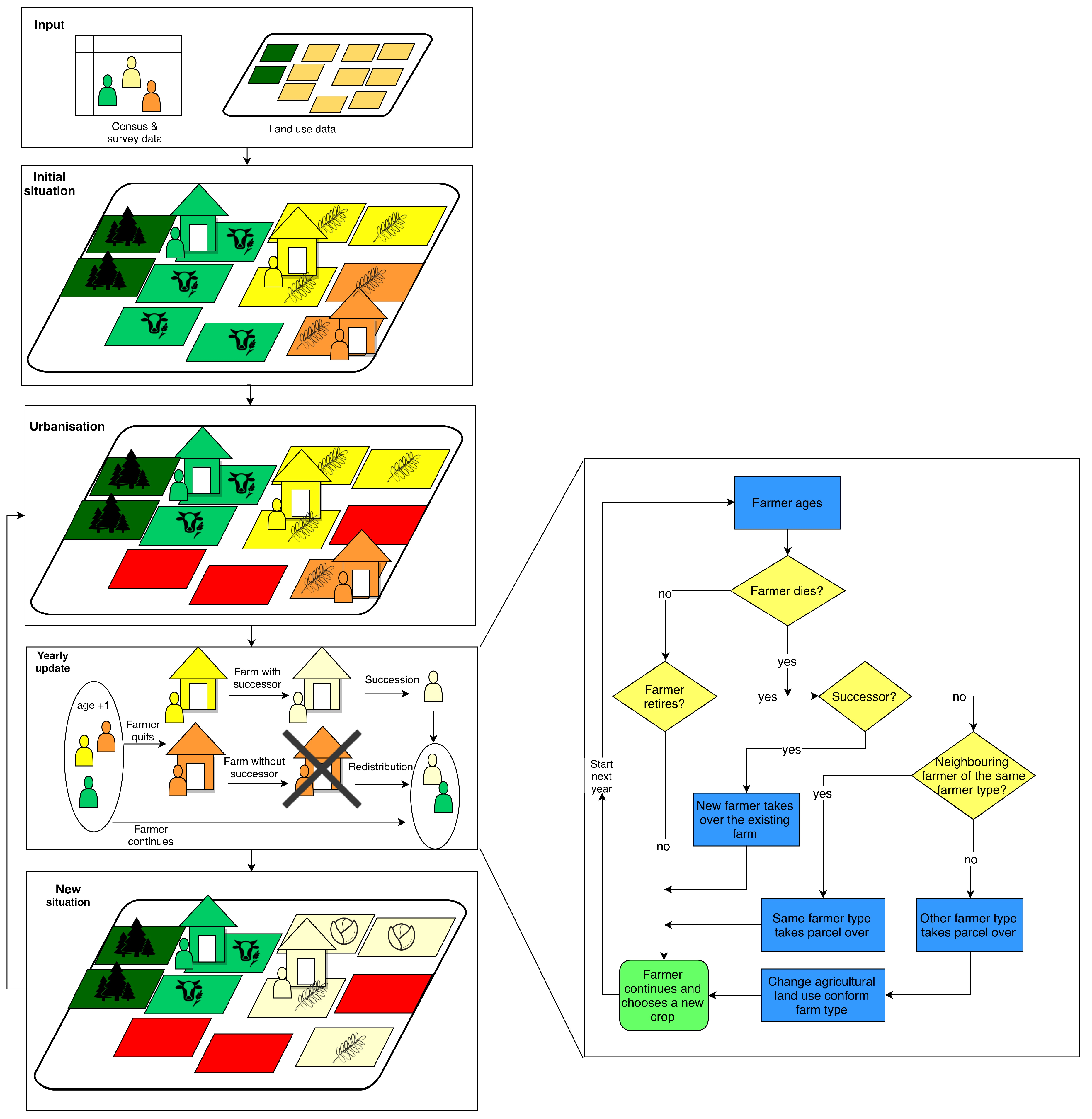
2. Description of the ADAM Model Framework

For the description of ABM’s, often the ODD-protocol (Overview—Design concepts—Details) developed by Grimm et al. [40,41] is used as a means to standardise descriptions of ABMs. It has previously been used by many authors to describe ABMs ever since it was published [39,42,43]. In this paper however, the model is presented in a descriptive manner, in order to explain the different steps in the model in a more consecutive order. For completeness, a summarized version following the ODD protocol is added in the Supplementary Materials as Table S2.
The ADAM model (Figure 1) is developed to represent the main processes driving agricultural land use change. It simulates the number of farmers, the size of farms, and the corresponding land use at the parcel level, trying to capture the main current processes of farms’ abandonment or growth. The model starts from a set of different types of farmers that are combined with agricultural parcels to create farms. The farmers and their farms have different characteristics, listed in Table 1: a farm is of a certain type and is managed by a farmer of a certain age. The farm consists of a number of parcels that, combined, form the entire farm and determine its size. The parcels are the agricultural parcels according to the datasets collected yearly as required by the EU in order to distinguish, identify, and measure the main crop production areas in Europe and check the validity of farmers’ applications for EU subsidies. A combination of internal (farm size, farm type) and external (market, policies, and physical environment) properties give the profitability of a farm. For model simplification purposes, farms only have one main farming type, and mixed farms were ignored.
The model is driven by the yearly decisions made by individual farmers. The decisions are based on a combination of the characteristics of the farm and define whether a new farm will be created, whether a farmer continues, stops its activities, or takes over an individual parcel or an entire farm. These decisions are steered by external factors such as the availability of new agricultural land, employment alternatives, and the reference wage in the region. Furthermore, the survival threshold for a farm, the characteristics of the parcels, the farmer’s age, and the availability of a successor also play a role in these decisions.
In the first phase, the land use of agricultural parcels is changed if spatial information is available (urbanisation, nature conservation, etc.). Next, all farmers decide whether they continue or stop farming. A farmer stops farming if he retires or dies or if his farm falls below a survival threshold. The farms of the farmers that stopped are taken over if the farmer has a successor: whether or not a farm has a successor is stochastically decided based on the succession rate in the region combined with the profitability of the farm. Those farms without a successor are split up and the individual parcels are taken over by farmers in the old farmers’ network, provided the agricultural land is suitable for the envisioned farming activities (e.g., fertility, existing infrastructure, local topography, and soil characteristics). The farmer’s neighbours are defined as the farmers who cultivate the parcels in the vicinity of the farmer. For the freed-up parcels, priority is given to farmers from the same farming type as the previous owner or a farmer who can easily convert the parcel to a desired agricultural land use (crop land, permanent crops, and grassland are easily converted, while greenhouses and agricultural buildings are more difficult and costly to convert). Currently, the price of the land is not included in this step.
These transformations are part of the last phase of the simulation where the agricultural land use is updated. This agricultural land use change can happen through (1) abandonment of unfavourable parcels when no new owner can be found, because the parcel is too far away from other parcels, (2) conversion to residential houses of farm houses, (3) changing cultivated crops on arable land stochastically by combining the probability of crop rotation cycles combined with expected yields for the area and crop prices and (4) converting the land to another type of agricultural land use when a farmer of another type acquires the parcel (e.g., through the removal of permanent crops or the conversion to pasture or the construction of agricultural buildings). The reasoning is that keeping the original agricultural land use requires important investments [44] and could lead to alienation from the farmer’s social network [45,46]. In order to apply the model to a certain region, data is needed on (1) the initial total farmer population, the age of these farmers, and their farm type; (2) the location of all agricultural parcels, the farmer cultivating each parcel and the current use of each parcel; (3) a list with for every parcel and the parcels in its vicinity; and (4) the typical crops or crop rotations present in the area together with their expected yield according to the local environmental characteristics.
Furthermore, other parameters need to be determined, namely, (1) the local average retirement age, together with the effective number of retirements at that age, (2) the mortality chance for farmers at every age, (3) the age of new-coming farmers, (4) the survival threshold of the farm, and (5) the chance of succession.
An illustration of setting up and running the model is given in the next part for the country of Belgium.

3. A Case Study for Belgium

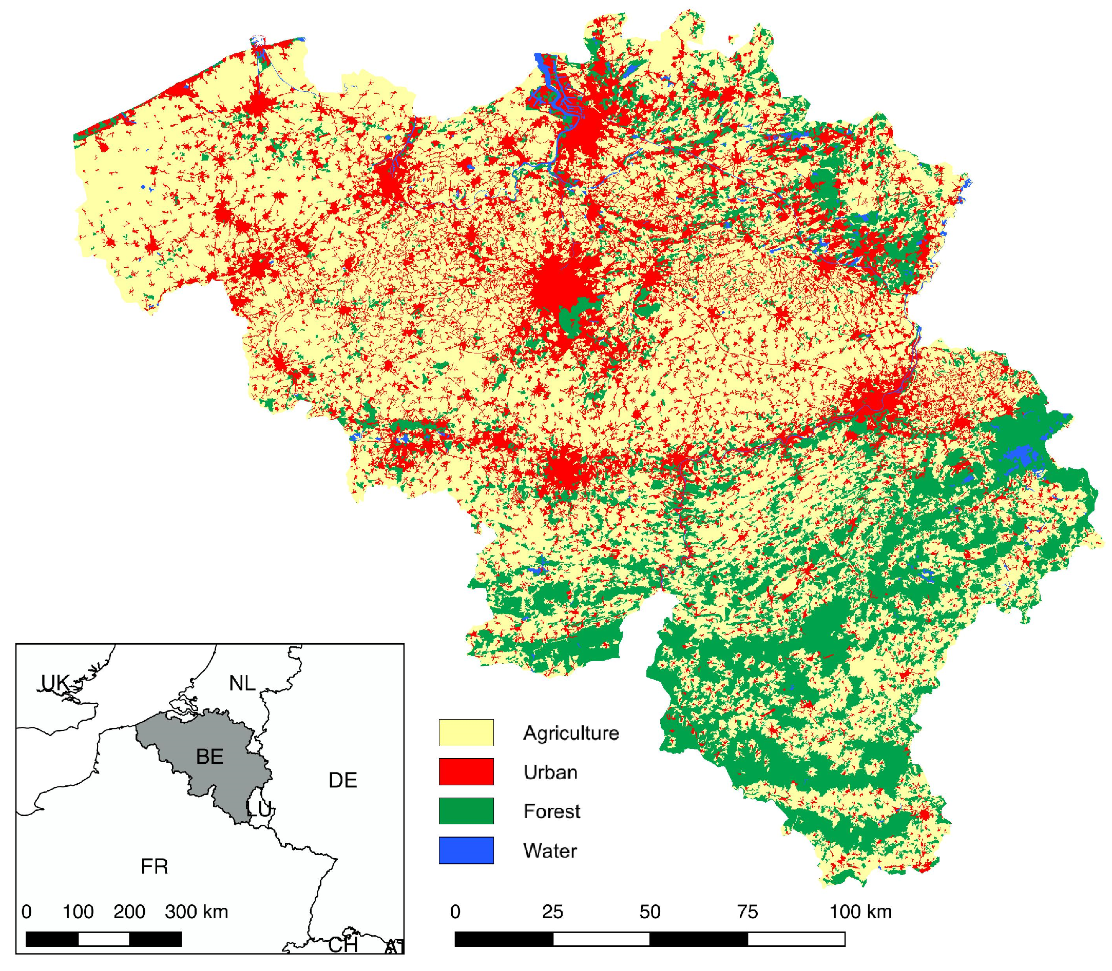
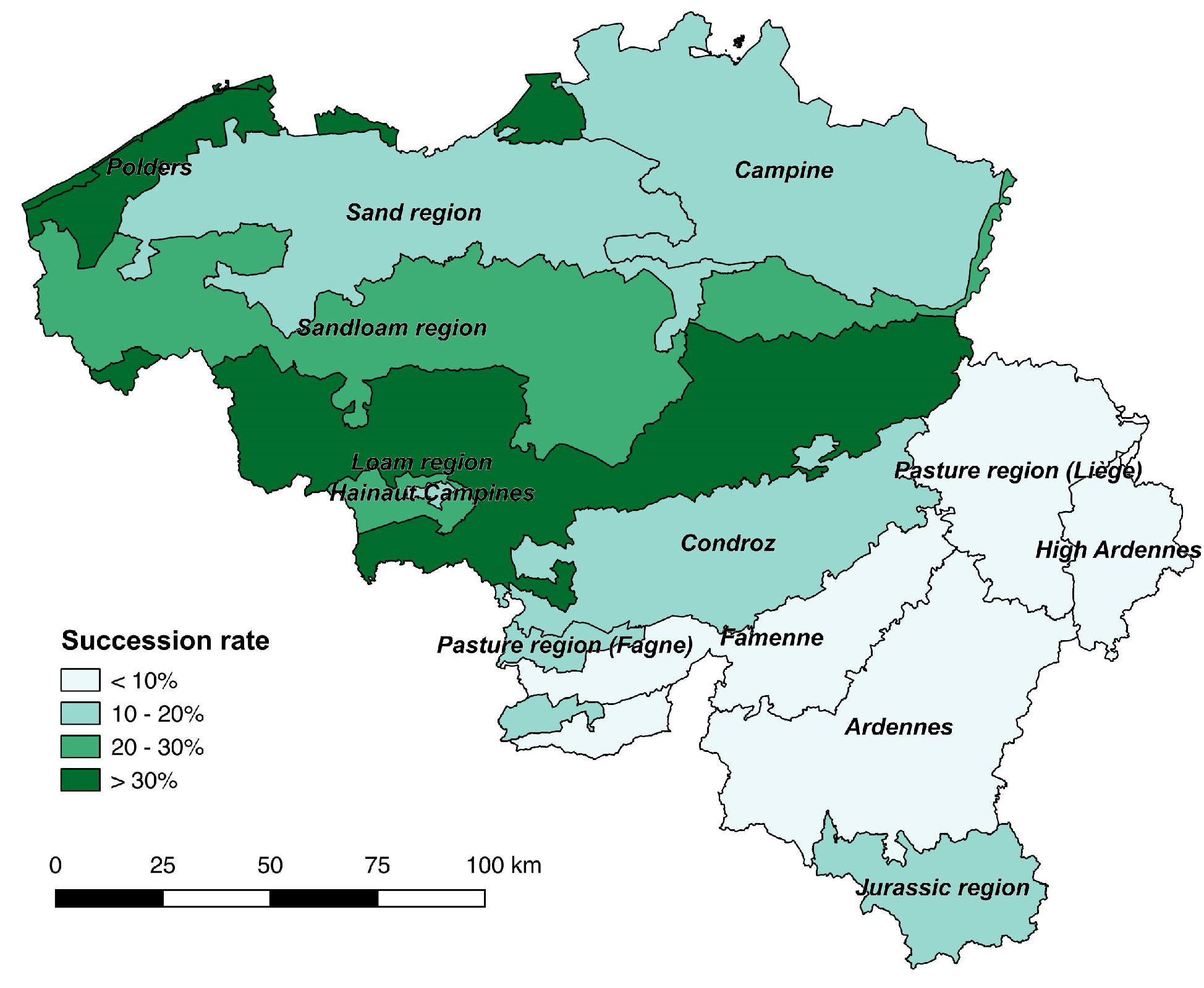
3.1. Study Area Background

In this section, the model is applied to the country of Belgium, situated in the centre of Western Europe (Figure 2). The highest percentages of cultivated areas in the country can be found in the central loam belt of the country and the northwest of the country, the Polders (Figure 2 and Figure 3). The Polders also has the highest density of farms. The Belgian Polder area dates from the Middle ages and is, due to its typical heavy soils, more suitable for animal-based farming (grasslands and fodder crops). Farms in the north-western part of the country are on average smaller than those in the east and south. This is a consequence of the population density before the industrialisation period in the south and the lower fertility of the soil in the east and south. Currently, the relation between population density and farm size is less prevalent [4].
Belgium has a long agrarian history, shaping the environment for centuries and leading to a great diversity of rural landscapes. Ever since the implementation of the Napoleonic inheritance law, heirs were to receive equal parts of the inheritance, leading to a strong fragmentation of the agricultural land [48]. The lack of spatial planning led to a rapid urbanisation of the countryside, increasing pressure on rural areas and open spaces, resulting in a strongly fragmented landscape. Former agricultural lands largely became residential areas, reducing space for farmers. The lack of space to grow encouraged farmers to intensify. This allowed them to keep earning a living on smaller and more fragmented parcel [4,13].
Despite these difficulties, the second half of the 20th century experienced an agricultural boom in Belgium as a result of technical progress and mechanisation, which increased productivity and turnover [4]. Additional support received through the first Common Agricultural Policy (CAP) of the EU also contributed to this boom. In parallel, noncompetitive and small farmers, unable to keep up with new necessary investments were driven out of agriculture. For the farmers that managed to continue farming, the pressure remains: urbanisation remains an attractive economic alternative to agricultural land and competition might further increase with the further phasing out of some of the trade barriers by the CAP under pressure of the WTO [48] and with the further decrease in subsidies from the CAP after 2020 [49,50]. Moreover, price fluctuations in the market can have a strong and immediate impact, and stricter environmental policies put new constraints on established farming techniques. Additionally, the possible role of climate change remains uncertain [4,11,51,52,53]. This requires farmers’ to constantly adapt and invest thus creating lasting land use changes on agricultural land. This continued pressure caused a further decline of farms by 70% between 1980 and 2015, an average of six farms per day [54]. A simple linear extrapolation of this trend would imply that no more farmers would remain by 2028 (Figure 4). Although this linear extrapolation is a simplification as the decrease might tail-off, it still gives a general idea on the speed of the decrease over the last decades and highlights the urgency of the necessity of a policy change, to curb this dramatic decline.
In contrast, total farmland area has only decreased slightly since 1980, resulting in an increase of the average farm size (Figure 5). Belgium is dominated by farms focusing on yearly rotating crops and herbivore farming. Greenhouse farming, permanent crop farming, and granivore farming are mostly found in Flanders, in the north of the country (Figure 6). The greenhouse and non-land-based farms can be related to the relative small farms in the north of the country which is a result of the high population density, urbanisation pressure, and the overall historical evolution of agriculture.
The sharp decrease in farmers’ numbers and large regional variation, characterized by a diverse landscape with diverse farming practices, together with a high competition for space, a high participation in the global market, and being part of the EU from the very beginning, makes Belgium representative for the general trends observed in Western-Europe and an interesting case study for the model.

3.2. Data

Data on the agricultural population was obtained from national agricultural surveys, which were collected on a yearly basis from 1970 onwards by the National Institute of Statistics of Belgium (NIS) [54]. The data of the survey of 2000 were used to create a realistic farmer population in the initialisation phase of the model. Later surveys were used to validate the modelled results.
Agricultural land use data were derived from the Système intégré de gestion et de contrôles (SIGEC) and Landbouwgebruikspercelen datasets for Wallonia and Flanders-Brussels, respectively, which are collected yearly as required by the EU [55]. This yearly collection is done in order to distinguish, identify, and measure the main crop production areas in Europe and check the validity of farmers’ applications for EU subsidies. The dataset contains the agricultural parcels as vector data, including the size of every parcel but without any information on ownership or right of use. The combined data for the year 2000 of Flanders, Brussels, and Wallonia were used to initialise the model.
Prices on the different modelled crops where obtained from the Food and Agriculture Organisation (FAO) dataset on annual producer prices [56] and where linearly extrapolated.

4. Model Initialisation and Calibration

4.1. Initialisation

As discussed in the last part of the methodology section, in order to apply the model, some initialisation of data and parameters is needed. The initial total farmer population and farmers’ type and age are derived from the agricultural surveys. The parcel location, current agricultural land use, typical crops, nearby parcels and crop rotations come from the agricultural parcel dataset. The crop rotations were extracted by creating a timeseries for the crops for each parcel in the available years for the parcel dataset and defining the probability that one crop is followed by another crop. These datasets are used to create the initial situation, since no information on the individual farmers and which parcels they cultivate is available. The first step in this initialisation is the creation of the different individual farmers of a certain age, located in a municipality, and who will manage a certain farm type with characteristics shown in Table 2. These different types of farmers currently only serve the purpose of making a distinction in the profitability and succession rate between different farming types. This distinction of farmer types, however, also allows to further refine the decision-making process in the future by adding differences in characteristics and behaviour. van Vliet et al. [57] stated the importance of the farmer characteristics when looking into agricultural land use change, and processes of intensification and disintensification. They were, however, found to be less important in the decision making process on whether or not a farmer decides to quit [57], and there is currently no data available that could be applied on the national scale in order to include this in the model. Once the farmer population is created, each farmer receives a first parcel as their home parcel. This parcel contains agricultural buildings according to the parcel dataset (or a random other parcel if there are not enough parcels with agricultural buildings). From this initial parcel, each farm starts growing by adding an agricultural parcel near the initial farm (defined as the 20 nearest parcels) that suit the farmer’s type (barns, grassland, greenhouses, permanent crops, or arable land). After each iteration, a new agricultural parcel, from the list of 20 nearest parcels of all parcels defining the farm, is added to the farm. The remaining parcels that could not be allocated to farms through this process, are randomly added to a neighbouring farm.
As mentioned before, apart from the initial dataset, other parameters need to be defined (see last part of methodology section). The local retirement age was set to 65, the legal retirement age in Belgium. Since many farmers continue farming even after they reach the legal retirement age (one third of EU farmers were 65 or older in 2013 [18]), a farmer only retires immediately at 65 if there is a successor. If there is no successor, farmers continue until they die, downsizing the farm in the meanwhile by giving up land they lease (about 2/3 of the total farmed area). Since no exact information is available on this chance of continuation after legal retirement age, the percentage is calibrated in the first model run. The mortality rates were defined using mortality statistics for the male Belgian population in 2000, aged 18 to 105, at which point the mortality rate is set to 100%. This dataset was chosen since, in Belgium, farmers are still mostly male (85% in 2000 [54]) and mortality rates differ between sexes at all ages. The age of the newcomer taking over a farm is set to a random age normally distributed around 30, with a standard deviation of five and a lower limit of 18 year.
For the Belgian case study, it is important to note that population density is high and land is rather scarce [58,59,60,61]. This results in a high demand for land, and farmland is hardly abandoned. There is almost always someone interested in taking over agricultural parcels that become available. If a successor is not found, neighbouring farmers take over the agricultural parcels and the farm house itself is converted to residential land use. The long agricultural history resulted in the most fertile lands being cultivated, while unfavourable plots have been abandoned. As such, the opening up of new agricultural land through, for example, deforestation, hardly happens in Belgium. Therefore, deforestation was not considered relevant and was not incorporated in the model. Furthermore, two open unstructured interviews with key experts in the government and the agricultural unions revealed that Belgian farmers in general do not quit farming unless they have a successor. Even when a farm is unsuccessful and falls below the survival threshold, farmers continue farming, even if this means living in poverty. Hence, the following assumptions where made for the Belgian case: newcomers can only enter the system by taking over another farm, a new cultivator can always be found for agricultural land that becomes available and a farmer continues farming at least until the retirement age, even if the farm is unprofitable.
In Belgium, no information is available on succession at the farm level from the Agricultural surveys. These surveys show however that for farmers over 50 years, only 15 to 16% are sure of having a successor, around 50% do not have a successor and the remaining 35% are unsure. These numbers vary greatly between agricultural areas, with higher succession certainty in fertile areas like the Polders and the Loam area (19% and 23%, respectively) and much lower in less fertile areas like the High Ardennes (4% having a successor, 74% having none). The decision for a successor to take over a farm was defined through the profitability of the farm. Defining the profitability of a farm requires complicated calculations and a large amount of specific information that is mostly unavailable. For land-based farming types, the profitability (as defined through the standard gross margins or SGM) is strongly correlated to the size of the farm on the municipality level (examples for cropland and dairy in Figure 7). Even though a linear regression between area and profitability is a simplification of reality and does not take into account many other factors contributing to the profitability of a farm, a linear regression between the area and the profitability at the municipality level was used as an approximation to define the profitability on the individual farm level (Profitability = area * slope). This profitability is then compared to the profitability of other farms through the mean and standard deviation. The succession chances (P(succ)) are then defined according to statistics for each agricultural region (Figure 3) corrected with a factor for the relative succession probability (Table 3).
For non-land-based agriculture, other factors such as the technological advancement and modernity are more important than the size in determining the succession probability. Since no data is available on the subject, for these types of farms, the average succession rate in the region was used, and farm size was not considered. Hence, for each farm, the probability of having a successor was assessed based on a combination of these factors.

4.2. Model Calibration

Most model inputs are derived from empirical data or defined through discussions with experts in the field (see above). As previously mentioned, data on retirement rate after passing the legal retirement age (65) are not available. In order to calibrate this percentage, the model was run for Belgium for yearly retirement percentages ranging from 10 to 30%. The yearly predicted results for the farmer population aged 65 and older between 2000 and 2010 were compared to the observed values from the Agricultural Surveys [54] for half of the municipalities. Results from after 2010 are available but from 2011 onwards, farmers could choose to be registered collectively in the survey. This option was given in order to simplify administrative work, but has led to a direct decrease of both the number of farmers and of the average farm size, which is derived from the number of farmers [62]. This change in methodology makes the comparison between observations and predictions difficult from 2011 onwards.
The predicted and observed data were evaluated by the means of a relative root mean square error (RRMSE).
  R M S E =   1 n i = 1 n ( m i o i ) 2  
  R R M S E = R M S E × 100 % o m e a n  
with n the number of observations, mi the modelled value, oi the observed value, and omean the mean of the observed values. The RRMSE gives insight on the difference between modelled and observed values, the lower the RRMSE value, the better the model performs. The model run with a retirement percentage of 14% was found to produce the lowest RRMSE (2.54%, Figure 8). This retirement probability was therefore used for subsequent simulations.

5. Results and Discussion
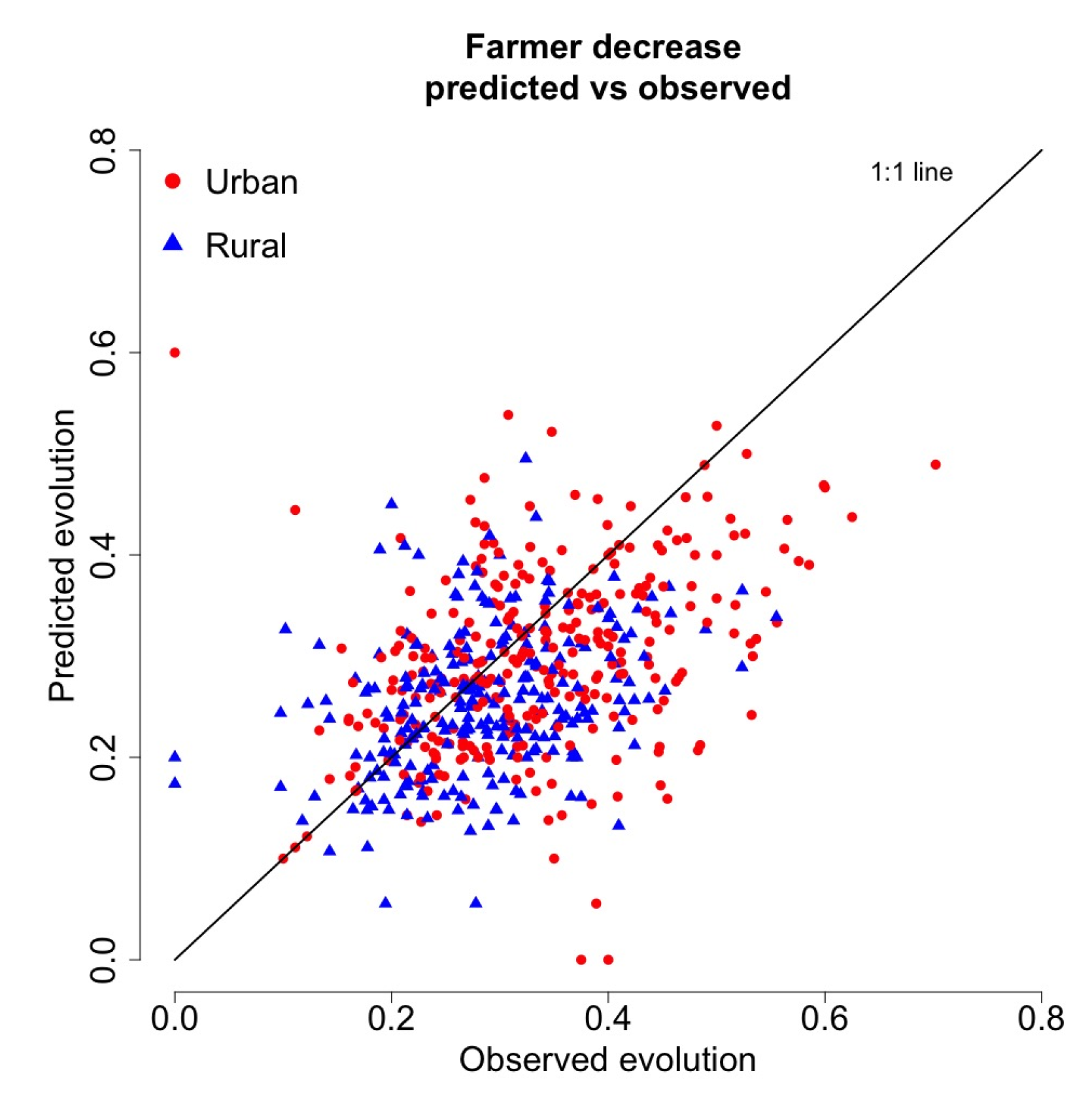
5.1. Validation

The initialisation phase resulted in a farm size distribution comparable to the farm distribution in Figure 5 for 2000, with an underestimation in the smallest category and an overestimation in the category 10–15 ha. However, these differences quickly disappear after a few years, creating a farm size distribution without important over- or underestimations.
The model was furthermore validated by comparing the predicted number of farmers for the time period ranging from 2000 to 2010 with observed data from the agricultural surveys [54] by means of the RRMSE. For the evolution of the total number of farmers in Belgium between 2000 and 2010, an RRMSE of 4.77% was obtained. These are promising results at the level of the entire Belgian farmer population, but possibly conceal discrepancies at the more detailed level of the municipality.
A municipality level comparison between observed and predicted number of farmers in 2010 results in an RRMSE of 5.11%. The observed versus predicted evolution of the number of farmers between 2000 and 2010 at the municipality level, results in an RRMSE of 46.4%. A scatterplot of these predicted and observed evolutions between 2000 and 2010 shows an R2 of 0.23. Both RRMSE and R2 show that the model is not performing adequately at the municipality level. However, splitting up the dataset between municipalities with less and more than 250 inhabitants per km2 shows that, while the rural municipalities (<250 people/km2) are rather equally spread, the more densely populated municipalities are more found under the 1:1 line (Figure 9). The difference in the mean observed decrease between rural and urban municipalities (0.28 vs. 0.35) also showed to be significant using a Student’s t-test with p < 0.05. This can most likely be explained by the fact that part of the municipalities with higher population densities are under pressure of urbanisation processes, especially municipalities located near large cities. These urbanisation processes, which decrease the amount of available agricultural land and so might make farms smaller (relative to other farms in the region) and therefore less interesting for succession, are currently not incorporated in the model. The proximity of larger cities might also provide alternative jobs for possible successors, making it harder for farmers to find one. Furthermore, urbanisation may complicate farming indirectly by making some parcels less accessible and through extra regulations to manage negative externalities (for example slow traffic, noise, and smells) [63]. The spatial variation in relative increase in farm size can largely be explained by the current farm sizes in these areas, which have the largest relative growth capacity.
Data for validation of the farm size and farm types are not available, due to privacy issues and recent changes in the methodology of the agricultural survey (see part 4.2).
The results on agricultural land use (Figure 10) match expectations on current agricultural land use in Belgium with the central loam belt mostly consisting of cropland, mostly grassland in the south of the country and a mix of crops and grassland in the north. A larger amount of agricultural buildings is present in the north-west, where the focus is mainly on granivore farming types. Permanent crops are strongly present in the east of the country north of the loam belt (Humid Hesbaye).

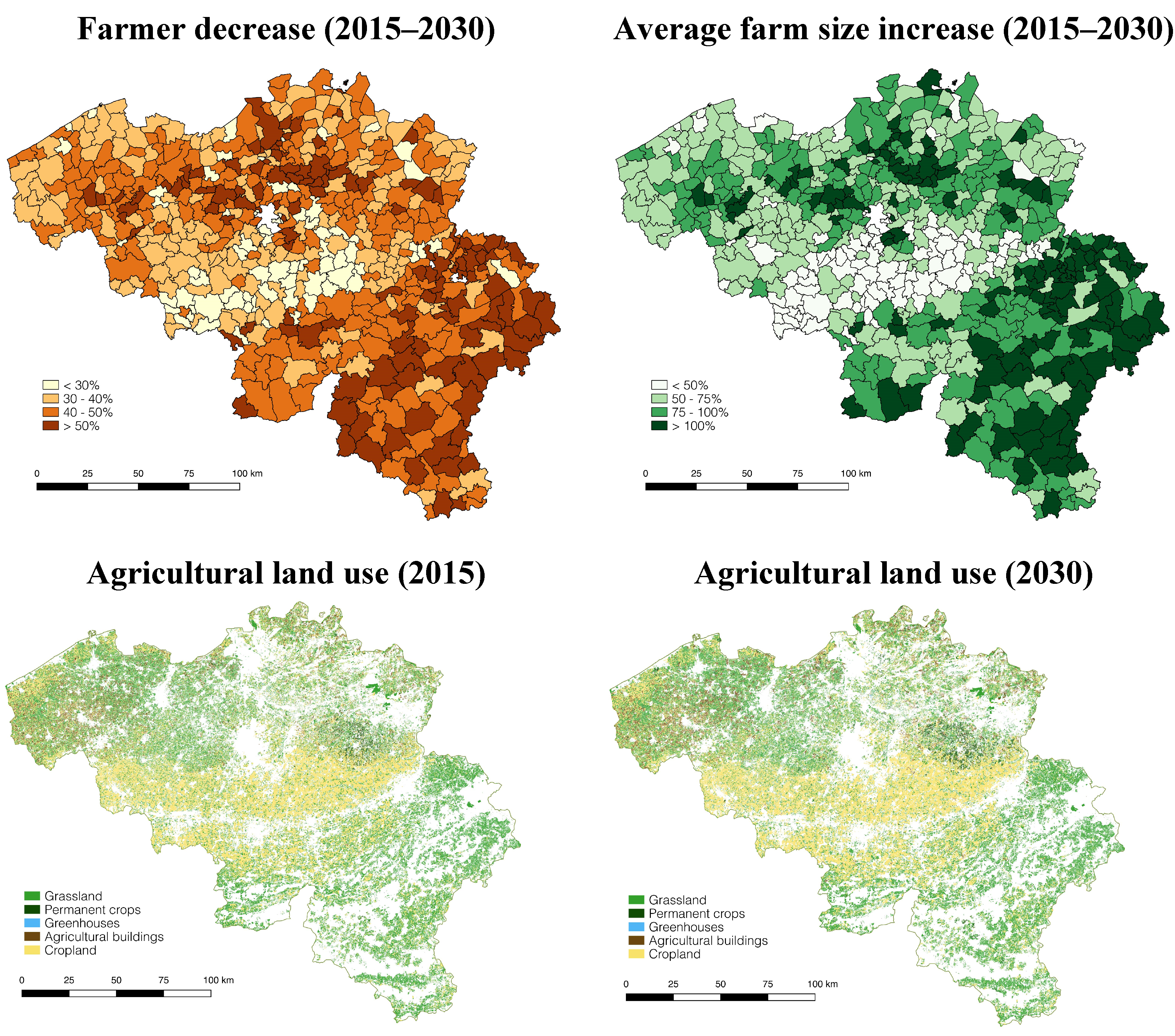
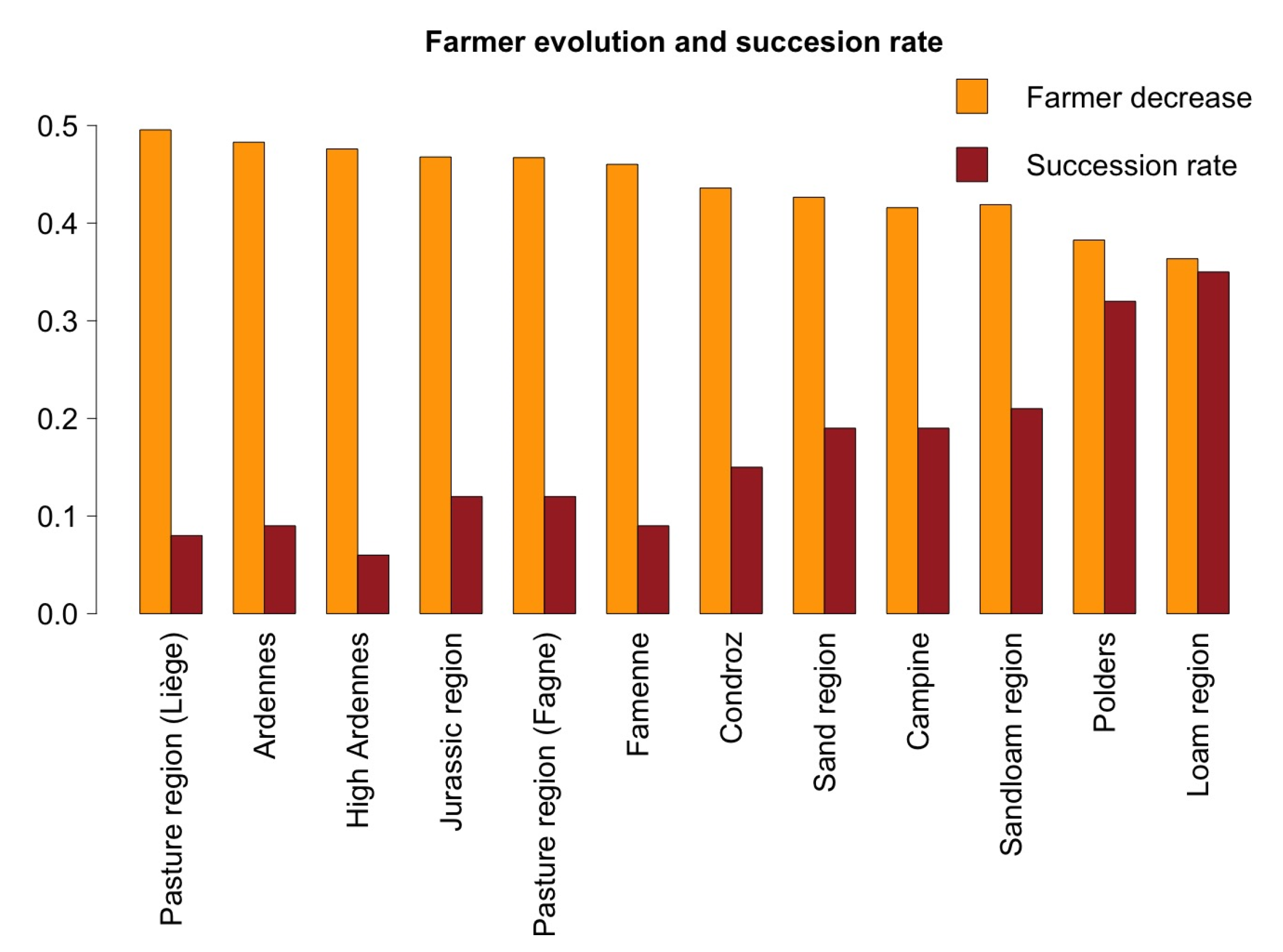
5.2. Simulations of a Business-as-Usual Scenario Until 2030

After calibration and validation for 2000–2010, the model was run until 2030 under a business-as-usual (BAU) scenario, under the assumption that current conditions and trends would continue in the future. The simulations show that the number of farmers keeps decreasing and that the average farm size continues to increase with small farms leaving the system, by being taken over by bigger farms.
These trends differ throughout the country. Results on the aggregated level of the municipality show that the percental decrease in number of farms is the lowest in the central part of the country and in the loam region (Figure 10). The relative size increase is the largest in the south and the central west part of the country. These results can be expected when comparing them with the average succession rate in Belgium for each agricultural region (Figure 3). This is especially the case in the centre of Belgium. This is the most fertile part of the country, where the succession rate is relatively high. In absolute terms, this is also the area where the largest farm increases can be found. The most apparent changes in agricultural land use change can be found in the central eastern part of the country with an increase in permanent crops and in the west with an increase in agricultural buildings.

5.3. Discussion

Ever since the start of the collection of farm data through agricultural surveys in Belgium a continuing trend of farmers decrease and farm size increase is observed, together with a decrease in mixed farming and an increase in monoculture farming systems. The most important driver of this change is the competition between farmers on the local and global level, requiring ever increasing intensification, rationalization, and growth.
The results from the BAU scenario indicate that farm size will continue to increase, with small farms disappearing, confirming the trend of growth for survival that is mentioned by Mazoyer & Roudart [13]. The disappearance of the small farms can lead to more personal dramas in farmer households that often have been living in hidden poverty for many years. The Belgian society could anticipate these changes by offering socio-ecological pathways out of their lock-in situation. A key challenge for the future of farming might be to be independent from fossil energy. The active of local farming and food systems could reduce the necessity to increase farm size in order to stay competitive in a global market.
Furthermore, this growth will lead to larger farms, sometimes creating larger parcels, whereby parcel boundaries might disappear as a successful farm takes over an adjacent parcel. This upscaling will lead to a decrease in the landscape diversity [14,15,16,17] and ecological value [64,65,66]. In current debates on the importance of ecology, ecosystem services and climate mitigation, these changes in landscape caused by current trends in agriculture, require an increased interest from policy makers and the creation of tools that allow the evaluation of different options in policy.
Our results demonstrate that ADAM is able to simulate the evolution of a farmer population, their farm size and the agricultural land use. The modelled (evolution of the) farmer population reproduces the observed trends and simulates a reliable agricultural population, making the model promising for use in future agent-based simulations of agricultural dynamics.
Running the model until 2030 under a BAU scenario shows the expected increase in average farm size throughout the country. Although the largest relative growth is expected in the north west of the country, the largest farms can still be found in the southern part of Belgium. This is due to the lower fertility of the soil, which historically already led to an on average larger farm size and still today results in an on average lower succession rate (Figure 11), ultimately leading to less farms being continued and a further growth of the remaining farms’.
The model currently uses only a limited number of farming types: yearly crop rotation farming, permanent crop farming, greenhouse farming, and land and barn-based animal farming. In reality however, some farmers perform agricultural side activities, while others have two or more main activities and are categorised as mixed farms in statistics. Ignoring the reality of mixed farming is another constraint of the model, which might need to be addressed in a next version. Furthermore, results for the agricultural land use could be further refined by improving the farmers’ decision making process by adding more differences in characteristics and behaviour. A broader range of farming types and greater detail on the agricultural land cover could provide more insights into the impact of the agricultural evolutions of ecosystem services related to agriculture.
Although the loss of agricultural land is limited (4% between 2000 and 2014), results show that local losses of agricultural land due to urbanisation are not negligible and must be included to improve the results of the model. Currently, a parcel containing the farm and the home of the farmer is no longer considered to be agricultural land but becomes a residential parcel and leaves the system. This type of urbanisation does not grasp the full reality of urbanisation of agricultural land. At the same time, this transformation from a farm to a residential home does not always match reality. Recently these farms have gained the interest of a new type of farmer, i.e., the peri-urban farmer, who produces for (and with) the local community. These farmers are interested in farms close to urban centres [67]. Although this is a recent and still relatively small trend, it might nevertheless be important in the process of urbanisation of agricultural land. Another interesting phenomenon is the usage of peri-urban farm land for horses by nonfarmers. These parcels are also considered to no longer be available for commercial farming.
The current agricultural land use change, (when a different farmer type than the previous takes over an agricultural parcel) does not consider the impact of land ownership versus rented land, even though this might hinder the farmer to alter the agricultural land use. In Belgium, only about 37% of land is owned by the farmer himself. This might have an impact on the agricultural land use change as it is currently presented in the model. During the rental period of the land, the renting farmer is however, protected by laws that allow farmers to have a long-term strategy for the land and their farm.
The aim of creating an agent-based model at the country scale, often with a limited amount of information, required a simplification of the decision-making process of the agents. This is because insight gained on agricultural decision making processes by previous studies [39,68,69,70,71], are often difficult to apply at country scale. This model framework, however, allows for the creation of a more detailed decision-making process when more information is available.
To summarise, ADAM allows for the simulation of the evolution of a farmer population. In further research, the model can be used under different scenarios and therefore evaluate the effects of different policies, different economic viewpoints, and a changing climate on different regions. For example, ADAM could be used to investigate the changes in expected yield as a consequence of different climate change scenarios, or the effect of subsidies on crop prices and to look on the effect these have on the decision-making process of the farmer. Another question that can be investigated by the model is how the farmer population reacts to changes in the legal retirement age or in changes in farmer subsidies, impacting the expected profitability of different farming types.
Despite the fact that ADAM can adequately simulate the evolution of a farmer population, improvements can still be made. This could be achieved by refining the farmers’ behaviour together with the farms’ typology (e.g., eco-farming and peri-urban farming). Additionally, further including regional differences and including the impact of urbanisation the on the availability of agricultural land would further improve the model.

6. Conclusions

In this paper, the agent-based model ADAM was presented. ADAM simulates the evolution of a farmer population at country scale, capturing basic farmer decision-making at the agent level, transcending the statistical level. As such, this research shows that it is possible to create agent-based models simulating real-world situations at the country level.
The study showed that ADAM performs less well in more densely populated communities. This can be explained by the fact that part of the municipalities with higher population densities are under pressure of urbanisation processes, especially municipalities located near large cities, but also by the fact that municipalities with higher population densities have less available room for agriculture, making the farms on average smaller and so more likely to disappear. Urbanisation thus leads to more rapid farm abandonment than expected. To address this issue, it would be useful to incorporate urbanisation data in the model, to see what the effect is on the farms and farmers.
ADAM was developed as a parsimonious model that captures the main processes driving agricultural land use change while excluding other relevant but small-scale processes such as the emergence of urban farming and horsification. ADAM is capable of adequately simulating an agricultural population, useful for further application in agent-based simulation of agricultural land use change. The model is capable of creating farms that evolve over time, outputting information on which agent manages a certain piece of land. As such, ADAM can be used to investigate the impact of different scenarios on the farm evolution and therefore on the profitability and succession rate of a farm. Increasing a farm size for economic reasons (e.g., as a consequence of the reduction of gross margins) is thought to be valid within a broad international context. Since the model uses data sets that are required for EU-reporting, the model can be applied in other EU-countries. The application in other countries will depend on local data availability. Evidently, many assumptions and parameters in the present model application for Belgium are region-specific. Application in other countries would require a recalibration and possibly a re-evaluation of certain assumptions made on farm succession, land availability, and land abandonment.

Supplementary Materials

The following are available online at https://www.mdpi.com/2073-445X/7/3/109/s1, Table S1. Non-exhaustive overview of agricultural simulation models in literature; Table S2. AD AM ODD protocol. References [72,73,74,75,76,77,78] are cited in the supplementary materials.

Author Contributions

Conceptualization: V.B., A.V.R., and N.D.; Methodology: V.B., M.V., E.V.H., A.V.R., and N.D.; Software: V.B. and J.B.; Validation: V.B.; Investigation: V.B.; Resources: V.B. and E.V.H.; Data curation: V.B. and J.B.; Writing—Original Draft Preparation: V.B.; Writing—Review & Editing: V.B., J.B., M.V., E.V.H., A.V.R. and N.D.; Visualisation: V.B.; Supervision: A.V.R. and N.D.; Project Administration: A.V.R. and N.D.; Funding Acquisition: N.D.

Funding

This research was funded by the Belgian Science Policy (BELSPO, Belgium)—Research project BR/121/A2/MASC.

Acknowledgments

The authors acknowledge the financial support of the Belgian Science Policy (BELSPO, Belgium). The authors thank the anonymous reviewers for their efforts and constructive comments which allowed us to improve the manuscript.

Conflicts of Interest

The authors declare no conflict of interest.

Model Information

The model is written in Java 8 and can be compiled with Javac 1.8.0_51. At runtime, an increased memory (using-Xmx4096m) is advised. No external dependencies are present. The code can be run via MainModel.java. Configuration parameters and data locations can be specified in Config.java. The code can be found at https://github.com/veroniquebeckers/ADAM.

References

  1. Anderson, K. Globalization’s effects on world agricultural trade, 1960–2050. Philos. Trans. R. Soc. B Biol. Sci. 2010, 365, 3007–3021. [Google Scholar] [CrossRef] [PubMed]
  2. FAO. The State of Food and Agriculture 2000—Lessons from the Past 50 Years; FAO: Rome, Italy, 2000; ISBN 9251044007. [Google Scholar]
  3. Altieri, M. Ecological impacts of industrial agriculture and the possibilities for truly sustainable farming. Mon. Rev. N. Y. 1998, 50, 60–71. [Google Scholar] [CrossRef]
  4. Van Hecke, E.; Antrop, M.; Schmitz, S.; Sevenant, M.; Van Eetvelde, V. Atlas van België—2 Landschap, Platteland en Landbouw; Academia Press: Gent, Belgium, 2010. [Google Scholar]
  5. Mather, A.S.; Fairbairn, J.; Needle, C.L. The course and drivers of the forest transition: The case of France. J. Rural Stud. 1999, 15, 65–90. [Google Scholar] [CrossRef]
  6. The World Bank. Agriculture for Development; The World Bank: Washington, DC, USA, 2008; Volume 54, ISBN 9780821368077. [Google Scholar]
  7. United States Department of Agriculture (USDA). National Agricultural Statistics Service Farms and Land in Farms; USDA: Washington, DC, USA, 2017; Volume 3, pp. 1995–2004.
  8. European Commission Small and Large Farms in the EU—Statistics from the Farm Structure Survey—Statistics Explained. Available online: http://ec.europa.eu/eurostat/statistics-explained/index.php/Small_and_large_farms_in_the_EU_-_statistics_from_the_farm_structure_survey (accessed on 2 October 2017).
  9. D’Odorico, P.; Carr, J.A.; Laio, F.; Ridolfi, L.; Vandoni, S. Feeding humanity through global food trade Earth’ s Future. Earth’s Future 2014, 2, 458–469. [Google Scholar] [CrossRef]
  10. Van Hecke, E. Revenus et Pauvreté dans L’Agriculture Wallonne; Fondation Roi Baudouin: Brussels, Belgium, 2001; ISBN 2-87212-335-0. [Google Scholar]
  11. Van Hecke, E.; Meert, H.; Christians, C. Belgian agriculture and rural environments. Belgeo 2000, 201–218. [Google Scholar] [CrossRef] [Green Version]
  12. Meert, H.; Vernimmen, T.; Bourgeois, M.; Van Huylenbroeck, G.; Van Hecke, E. Erop of Eronder: Bestaans(on)zekere Boeren en hun Overlevingsstrategieën; Koning Boudewijn Stichting: Brussels, Belgium, 2002; ISBN 90-5130-410-2. [Google Scholar]
  13. Mazoyer, M.; Roudart, L. A History of World Agriculture: From the Neolithic Age to the Current Crisis; NYU Press: New York, NY, USA, 2006; ISBN 9781844074006. [Google Scholar]
  14. Harms, W.B.; Stortelder, A.H.F.; Vos, W. Effects of Intensification of Agriculture on Nature and Landscape in the Netherlands. Ekológia 1984, 3, 281–304. [Google Scholar]
  15. Ihse, M. Swedish agricultural landscapes—Patterns and changes during the last 50 years, studied by aerial photos. Landsc. Urban Plan. 1995, 31, 21–37. [Google Scholar] [CrossRef]
  16. Poudevigne, I.; Alard, D. Landscape and agricultural patterns in rural areas: A case study in the Brionne Basin, Normandy, France. J. Environ. Manag. 1997, 50, 335–349. [Google Scholar] [CrossRef]
  17. Björklund, J.; Limburg, K.E.; Rydberg, T. Impact of production intensity on the ability of the agricultural landscape to generate ecosystem services: An example from Sweden. Ecol. Econ. 1999, 29, 269–291. [Google Scholar] [CrossRef]
  18. Eurostat. Farm Structure Survey 2013; Eurostat: Kirchberg, Luxembourg, 2015; Volume 206. [Google Scholar]
  19. European Commission. The Common Agricultural Policy; European Commission: Luxembourg, 2012; Volume 24. [Google Scholar]
  20. USDA. U.S. Farm Policy: The First 200 Years; USDA: Washington, DC, USA, 2002; pp. 21–25.
  21. Headey, D.D. The evolution of global farming land: Facts and interpretations. Agric. Econ. 2016, 47, 185–196. [Google Scholar] [CrossRef]
  22. Lerman, Z.; Kislev, Y.; Biton, D.; Kriss, A. Agricultural Output and Productivity in the Former Soviet Republics. Econ. Dev. Cult. Chang. 2003, 51, 999–1018. [Google Scholar] [CrossRef]
  23. Alston, J.M.; Babcock, B.A.; Pardey, P.G. The Shifting Patterns of Agricultural Production and Productivity Worldwide; Midwest Agribusiness Trade Research and Information Center: Ames, IA, USA, 2010; ISBN 978-0-9624121-8-9. [Google Scholar]
  24. Beddow, J.M.; Pardey, P.G. Moving Matters: The Effect of Location on Crop Production. J. Econ. Hist. 2015, 75, 219–249. [Google Scholar] [CrossRef]
  25. Rivers, N.; Schaufele, B. The effect of carbon taxes on agricultural trade. Can. J. Agric. Econ. 2014, 63, 235–257. [Google Scholar] [CrossRef]
  26. FAO. The Future of Food and Agriculture—Trends and Challenges; FAO: Rome, Italy, 2017. [Google Scholar]
  27. Westhoek, H.J.; Van Den Berg, M.; Bakkes, J.A. Scenario development to explore the future of Europe’s rural areas. Agric. Ecosyst. Environ. 2006, 114, 7–20. [Google Scholar] [CrossRef]
  28. Alexandratos, N.; Bruinsma, J. World agriculture: Towards 2015/2030: An FAO perspective. Land Use Policy 2003, 20, 375. [Google Scholar] [CrossRef]
  29. Spangenberg, J.H.; Fronzek, S.; Hammen, V.; Hickler, T.; Jäger, J.; Jylhä, K.; Kühn, I.; Marion, G.; Maxim, L.; Monterroso, I.; et al. The ALARM Scenarios: Storylines and Simulations for Assessing Biodiversity Risks in Europe. In Atlas Biodivers. Risk; Pensoft: Sofia, Bulgaria, 2010; pp. 10–15. ISBN 9789546424471. [Google Scholar]
  30. Brown, C.; Murray-Rust, D.; Van Vliet, J.; Alam, S.J.; Verburg, P.H.; Rounsevell, M.D. Experiments in globalisation, food security and land use decision making. PLoS ONE 2014, 9, 1–24. [Google Scholar] [CrossRef] [PubMed] [Green Version]
  31. Berger, T. Agent-based spatial models applied to agriculture: A simulation tool for technology diffusion, resource use changes and policy analysis. Agric. Econ. 2001, 25, 245–260. [Google Scholar] [CrossRef]
  32. Parker, D.C.; Berger, T.; Manson, S.M. Agent-Based Models of Land-Use and Land-Cover Change. LUCC Rep. Ser. 2002, 140, 4–7. [Google Scholar]
  33. Bousquet, F.; Le Page, C. Multi-agent simulations and ecosystem management: A review. Ecol. Modell. 2004, 176, 313–332. [Google Scholar] [CrossRef]
  34. Parker, D.C.; Manson, S.M.; Berger, T. Potential strengths and appropriate roles for ABM/LUCC. In Proceedings of the Special Workshop on Agent-Based Models of Land-Use/Land-Cover Change (CIPEC/CSISS), Santa Barbara, CA, USA, 4–7 October 2001; pp. 17–24. [Google Scholar]
  35. Parker, D.C.; Manson, S.M.; Janssen, M.A.; Hoffmann, M.J.; Deadman, P. Multi-Agent Systems for the Simulation of Land-Use and Land-Cover Change: A Review. Ann. Assoc. Am. Geogr. 2002, 75. [Google Scholar] [CrossRef]
  36. Schelling, T.C. Dynamic models of segregation. J. Math. Sociol. 1971, 1, 143–186. [Google Scholar] [CrossRef]
  37. Murray-Rust, D.; Brown, C.; van Vliet, J.; Alam, S.J.; Robinson, D.T.; Verburg, P.H.; Rounsevell, M. Combining agent functional types, capitals and services to model land use dynamics. Environ. Model. Softw. 2014, 59, 187–201. [Google Scholar] [CrossRef]
  38. Murray-Rust, D.; Dendoncker, N.; Dawson, T.P.; Acosta-Michlik, L.; Karali, E.; Guillem, E.; Rounsevell, M. Conceptualising the analysis of socio-ecological systems through ecosystem services and agent-based modelling. J. Land Use Sci. 2011, 6, 83–99. [Google Scholar] [CrossRef]
  39. Bakker, M.M.; Jamal, S.; Van Dijk, J.; Rounsevell, M.D.A. Land-use change arising from rural land exchange: An agent-based simulation model. Landsc. Ecol. 2015, 30, 273–286. [Google Scholar] [CrossRef]
  40. Grimm, V.; Berger, U.; Bastiansen, F.; Eliassen, S.; Ginot, V.; Giske, J.; Goss-Custard, J.; Grand, T.; Heinz, S.K.; Huse, G.; et al. A standard protocol for describing individual-based and agent-based models. Ecol. Modell. 2006, 198, 115–126. [Google Scholar] [CrossRef]
  41. Grimm, V.; Berger, U.; DeAngelis, D.L.; Polhill, J.G.; Giske, J.; Railsback, S.F. The ODD protocol: A review and first update. Ecol. Modell. 2010, 221, 2760–2768. [Google Scholar] [CrossRef] [Green Version]
  42. Bert, F.E.; Podestá, G.P.; Rovere, S.L.; Menéndez, Á.N.; North, M.; Tatara, E.; Laciana, C.E.; Weber, E.; Toranzo, F.R. An agent based model to simulate structural and land use changes in agricultural systems of the argentine pampas. Ecol. Modell. 2011, 222, 3486–3499. [Google Scholar] [CrossRef]
  43. Yamashita, R.; Hoshino, S. Development of an agent-based model for estimation of agricultural land preservation in rural Japan. Agric. Syst. 2018, 164, 264–276. [Google Scholar] [CrossRef]
  44. Rounsevell, M.D.A.; Annetts, J.E.; Audsley, E.; Mayr, T.; Reginster, I. Modelling the spatial distribution of agricultural land use at the regional scale. Agric. Ecosyst. Environ. 2003, 95, 465–479. [Google Scholar] [CrossRef]
  45. Karali, E.; Brunner, B.; Doherty, R.; Hersperger, A.M.; Rounsevell, M.D.A. The Effect of Farmer Attitudes and Objectives on the Heterogeneity of Farm Attributes and Management in Switzerland. Hum. Ecol. 2013, 41, 915–926. [Google Scholar] [CrossRef]
  46. Karali, E.; Brunner, B.; Doherty, R.; Hersperger, A.; Rounsevell, M. Identifying the Factors That Influence Farmer Participation in Environmental Management Practices in Switzerland. Hum. Ecol. 2014, 42, 951–963. [Google Scholar] [CrossRef]
  47. Büttner, G.; Soukup, T.; Kosztra, B. Addendum to CLC2006 Technical Guidelines; Copernicus Land Monitoring Service: Malaga, Spain, 2014; Volume 2, pp. 1–35. [Google Scholar]
  48. Mathijs, E.; Relaes, J. Landbouw en Voedsel, Verrassend Actueel; Acco: Leuven, Belgium, 2012; ISBN 9033480956. [Google Scholar]
  49. European Council. Reform of the Common Agriculturla Policy. Available online: http://www.consilium.europa.eu/en/policies/cap-reform/ (accessed on 6 September 2018).
  50. European Commission. EU Budget: The Common Agricultural Policy beyond 2020. Available online: http://europa.eu/rapid/press-release_IP-18-3985_en.htm (accessed on 6 September 2018).
  51. Olesen, J.E.; Bindi, M. Consequences of climate change for European agricultural productivity, land use and policy. Eur. J. Agron. 2002, 16, 239–262. [Google Scholar] [CrossRef]
  52. Maertens, E. Agromilieumaatregelen: Hoe Denken Landbouwers Erover? Departement Landbouw en Visserij: Brussels, Belgium, 2011. [Google Scholar]
  53. Van Passel, S.; Massetti, E.; Mendelsohn, R. A Ricardian Analysis of the Impact of Climate Change on European Agriculture. Environ. Resour. Econ. 2017, 67, 725–760. [Google Scholar] [CrossRef]
  54. Statistics Belgium. Agricultural Surveys from 1980–2015; Statistics Belgium: Brussels, Belgium, 2015.
  55. European Commission. Integrated Administration and Control System (IACS). Available online: https://ec.europa.eu/agriculture/direct-support/iacs_en (accessed on 6 September 2018).
  56. Food and Agriculture Organization Producer Prices—Annual. Available online: http://www.fao.org/faostat/en/#data/PP (accessed on 3 June 2018).
  57. Van Vliet, J.; de Groot, H.L.F.; Rietveld, P.; Verburg, P.H. Manifestations and underlying drivers of agricultural land use change in Europe. Landsc. Urban Plan. 2015, 133, 24–36. [Google Scholar] [CrossRef]
  58. Poelmans, L.; Van Rompaey, A. Detecting and modelling spatial patterns of urban sprawl in highly fragmented areas: A case study in the Flanders-Brussels region. Landsc. Urban Plan. 2009, 93, 10–19. [Google Scholar] [CrossRef]
  59. Mustafa, A.; Van Rompaey, A.; Cools, M.; Saadi, I.; Teller, J. Addressing the determinants of built-up expansion and densification processes at the regional scale. Urban Stud. 2018, 0042098017749176. [Google Scholar] [CrossRef]
  60. Mollen, F.H. Beton Rapport van de Vlaamse Gemeenten en Provincies; Natuurpunt: Mechelen, Belgium, 2018. [Google Scholar]
  61. Bouchedor, A. Pressions sur nos Terres Agricoles; FIAN Belgium: Brussels, Belgium, 2017. [Google Scholar]
  62. Departement Landbouw en Visserij. Landbouwrapport 2014; Departement Landbouw en Visserij: Brussels, Belgium, 2014. [Google Scholar]
  63. Delbecq, B.A.; Florax, R. Farmland allocation along the rural-urban gradient: The impacts of urbanization and urban sprawl. In Proceedings of the Agricultural and Applied Economics Association 2010 Annual Meeting, Denver, CO, USA, 25–27 July 2010; pp. 25–27. [Google Scholar]
  64. Marshall, E.J.P.; Moonen, A.C. Field margins in northern Europe: Their functions and interactions with agriculture. Agric. Ecosyst. Environ. 2002, 89, 5–21. [Google Scholar] [CrossRef]
  65. Stoate, C.; Boatman, N.D.; Borralho, R.J.; Carvalho, C.R.; de Snoo, G.R.; Eden, P. Ecological impacts of arable intensification in Europe. J. Environ. Manag. 2001, 63, 337–365. [Google Scholar] [CrossRef]
  66. Benton, T.G.; Vickery, J.A.; Wilson, J.D. Farmland biodiversity: Is habitat heterogeneity the key? Trends Ecol. Evol. 2003, 18, 182–188. [Google Scholar] [CrossRef]
  67. Danckaert, S.; Cazaux, G.; Bas, L.; Van Gijseghem, D. Landbouw in een Groen en Dynamisch Stedengewest; Departement Landbouw en Visserij, afdeling Monitoring en Studie: Brussel, Belgium, 2010; Volume 66. [Google Scholar]
  68. Fontaine, C.M.; Rounsevell, M.D.A. An Agent-based approach to model future residential pressure on a regional landscape. Landsc. Ecol. 2009, 24, 1237–1254. [Google Scholar] [CrossRef]
  69. Verburg, P.H.; Soepboer, W.; Veldkamp, A.; Limpiada, R.; Espaldon, V.; Mastura, S.S.A. Modeling the spatial dynamics of regional land use: The CLUE-S model. Environ. Manag. 2002, 30, 391–405. [Google Scholar] [CrossRef] [PubMed]
  70. De Lauwere, C.C. The role of agricultural entrepreneurship in Dutch agriculture of today. Agric. Econ. 2005, 33, 229–238. [Google Scholar] [CrossRef]
  71. Van Vliet, J.; Magliocca, N.R.; Büchner, B.; Cook, E.; Rey Benayas, J.M.; Ellis, E.C.; Heinimann, A.; Keys, E.; Lee, T.M.; Liu, J.; et al. Meta-studies in land use science: Current coverage and prospects. Ambio 2016, 45, 15–28. [Google Scholar] [CrossRef] [PubMed] [Green Version]
  72. Veldkamp, A.; Fresco, L.O. CLUE: A conceptual model to study the Conversion of Land Use and its Effects. Ecol. Modell. 1996, 85, 253–270. [Google Scholar] [CrossRef]
  73. Verburg, P.H.; Overmars, K.P. Combining top-down and bottom-up dynamics in land use modeling: Exploring the future of abandoned farmlands in Europe with the Dyna-CLUE model. Landsc. Ecol. 2009, 24, 1167–1181. [Google Scholar] [CrossRef]
  74. Sohl, T.; Sayler, K. Using the FORE-SCE model to project land-cover change in the southeastern United States. Ecol. Modell. 2008, 219, 49–65. [Google Scholar] [CrossRef]
  75. Soares-Filho, B.S.; Coutinho Cerqueira, G.; Lopes Pennachin, C. DINAMICA—A stochastic cellular automata model designed to simulate the landscape dynamics in an Amazonian colonization frontier. Ecol. Modell. 2002, 154, 217–235. [Google Scholar] [CrossRef]
  76. Thornton, P.K.; Jones, P.G. A conceptual approach to dynamic agricultural land-use modelling. Agric. Syst. 1998, 57, 505–521. [Google Scholar] [CrossRef]
  77. Schaldach, R.; Alcamo, J.; Koch, J.; Kölking, C.; Lapola, D.M.; Schüngel, J.; Priess, J.A. An integrated approach to modelling land-use change on continental and global scales. Environ. Model. Softw. 2011, 26, 1041–1051. [Google Scholar] [CrossRef]
  78. Van Meijl, H.; Van Rheenen, T.; Tabeau, A.; Eickhout, B. The impact of different policy environments on agricultural land use in Europe. Agric. Ecosyst. Environ. 2006, 114, 21–38. [Google Scholar] [CrossRef]
Figure 1. Overview of the Agricultural Dynamics through Agent-based Modelling (ADAM) model.
Land 07 00109 g001
Figure 2. Land use in Belgium according to classification of Corine Land Cover data [47].
Land 07 00109 g002
Figure 3. Succession rate for agricultural regions in Belgium.
Land 07 00109 g003
Figure 4. Evolution of the number of farmers in Belgium between 1980 and 2015 and a linear extrapolation of the trend.
Land 07 00109 g004
Figure 5. Evolution of the farm size distribution as a percentage of the total amount of farms from 1980–2014 in Belgium based on data from the agricultural surveys.
Land 07 00109 g005
Figure 6. Number of farmers of each type in Belgium, Flanders, and Wallonia.
Land 07 00109 g006
Figure 7. Relation between average standard gross margins (SGM) and average farm size for cropland (left) and dairy farming (right) in Belgium on the municipality level.
Land 07 00109 g007
Figure 8. Calibration through the relative root mean square error (RRMSE) for different percentages of retirement after legal retirement age.
Land 07 00109 g008
Figure 9. Observed vs. predicted percentage of farmer decrease between 2000 and 2010.
Land 07 00109 g009
Figure 10. Results of runs of the model until 2030 with the percentage of decrease of number of farmers between 2015 and 2020 (upper left), the percentage increase of farm size between 2015 and 2030 (upper right) and the agricultural land use in 2015 (lower left) and 2030 (lower right).
Land 07 00109 g010
Figure 11. Percentage decrease of farmers between 2015 and 2030 and the succession rate used for each agricultural region.
Land 07 00109 g011
Table 1. Overview of the different variables representing the characteristics of farms and farmers in the model.
VariableVariable TypeUpdate
Farm typeCategorical variable related to the type of farming practiceFarm type can change when new farmer takes over
Age of farmerNumerical variableYearly update, changes when farmer is succeeded
ParcelGeographical variable (polygon with location and size)Farmer and type (agricultural land use) can change if parcels are taken over
Farm sizeNumerical: sum of size of parcels farmed by a farmerIncreases when farmer takes over other parcels
Table 2. Characteristics of different farm types.
Farm TypeMain Parcel TypeCommon Agricultural Product
Yearly rotating crop farmersArable land with temporary cropsWheat, barley, maize, beets, potatoes, rapeseed
Greenhouse farmersGreenhousesTomatoes, bell peppers, cucumbers, zucchinis, strawberries, flowers
Barn based animal farmerBarns and croplandMeat (pork & poultry) & eggs
Land based animal farmerBarns, grassland, and croplandMeat (beef), milk
Permanent crop farmersArable land with permanent cropsApples, pears, cherries
Table 3. Relation between the profitability and the succession probability.
Profitability > (μ + SD * 2.5) P(succ) = regionalSurvChance * 4
Profitability > (μ + SD * 1.5) P(succ) = regionalSurvChance * 3
Profitability > (μ + SD * 0.5)P(succ) = regionalSurvChance * 2
Profitability > (μ − SD * 0.5)P(succ) = regionalSurvChance * 1
Profitability > (μ − SD * 0.75)P(succ) = regionalSurvChance * 0.5
Profitability < (μ − SD * 0.75)P(succ) = regionalSurvChance * 0.1

