Article

Analysis and Prediction of Land Use Changes Related to Invasive Species and Major Driving Forces in the State of Connecticut

1
Department of Geography, University of Connecticut, 215 Glenbrook Rd, Storrs, CT 06269, USA
2
Department of Natural Resources and the Environment, University of New Hampshire, 56 College Road, Durham, NH 03824, USA
3
Department Economics, University of Connecticut, 365 Fairfield Way, Storrs, CT 06269, USA
4
Department of Ecology and Evolutionary Biology, University of Connecticut, 75 N. Eagleville Road, Storrs, CT 06269, USA
*
Author to whom correspondence should be addressed.
Submission received: 14 March 2016 / Revised: 28 June 2016 / Accepted: 22 July 2016 / Published: 28 July 2016

Abstract

:
Land use and land cover (LULC) patterns play an important role in the establishment and spread of invasive plants. Understanding LULC changes is useful for early detection and management of land-use change to reduce the spread of invasive species. The primary objective of this study is to analyze and predict LULC changes in Connecticut. LULC maps for 1996, 2001 and 2006 were selected to analyze past land cover changes, and then potential LULC distribution in 2018 was predicted using the Multi-Layer Perceptron Markov Chain (MLP_MC) model. This study shows that the total area of forest has been decreasing, mainly caused by urban development and other human activity in Connecticut. The model predicts that the study area will lose 5535 ha of deciduous forest and gain 3502 ha of built-up area from 2006 to 2018. Moreover, forests near built-up areas and agriculture lands appear to be more vulnerable to conversion. Changes in LULC may result in subtle spatial shifts in invasion risk by an abundant invasive shrub, Japanese barberry (Berberis thunbergii). The gain of developed areas at the landscape scale was most closely linked to increased future invasion risk. Our findings suggest that the forest conversion needs to be controlled and well managed to help mitigate future invasion risk.

Graphical Abstract

1. Introduction

Woody alien plants are particularly important in the Northeastern United States: they make up 32% of the invasive plant species in the region and constitute about 70% of the invasive plant occurrence records [1]. In Connecticut, invasive species constitute a high percentage of the vascular plant flora, and have created ecological damage and economic losses [1,2,3,4]. The current flora is composed of 35% percent nonindigenous species [3]. The main invasive species impacts include direct and indirect economic costs to property, human health, and ecosystem services [5,6,7,8,9,10]. The cost to control invasive species and the damages they inflicted upon properties and natural resources in the U.S. is estimated at $137 billion annually [11]. In addition, these invasive species pose an important threat to biodiversity in Connecticut [3]. Invasive plants co-occur with nearly half of rare plant species in New England, and are most frequent and diverse in Connecticut among all New England states [7].
One especially problematic invasive plant in Connecticut is Berberis thunbergii (Japanese barberry). This perennial woody shrub provides excellent habitats for Lyme-disease carrying ticks thereby increasing the risk of infection in humans [12,13] in addition to altering ecosystem functions, such as nitrogen cycling, in invaded areas [14]. Japanese barberry was the second most frequently observed invasive plant at rare species sites in New England, and invasive plant presence was correlated with decreases in rare species population size [7]. Predicting future changes in invasion probability for Japanese barberry could help direct management efforts to mitigate its effects.
Land use patterns play an important role in the establishment and spread of invasive plants. Land use changes can aid plant invasions by promoting disturbances that may be a key to establishment, by creating habitats that may be more favorable to particular species, and also by creating dispersal corridors [15,16]. Therefore, incorporating land use change is a priority in models forecasting future invasions. Previous studies suggested that land use changes provide opportunities for particular plants to invade an area [17,18,19], that the types of changes that promote one species might inhibit others [18], and that land use changes contribute not only to invasive species establishment but also to their spread [20,21]. The generation of forest edges and the fragmentation of contiguous forest habitats are particularly important to woody invasive plant richness [22]. There are no studies, however, that analyze and predict future land use changes related to invasive species that might help predict the spatial distribution of future invasive species based on the predicted land use and land cover (LULC) data.
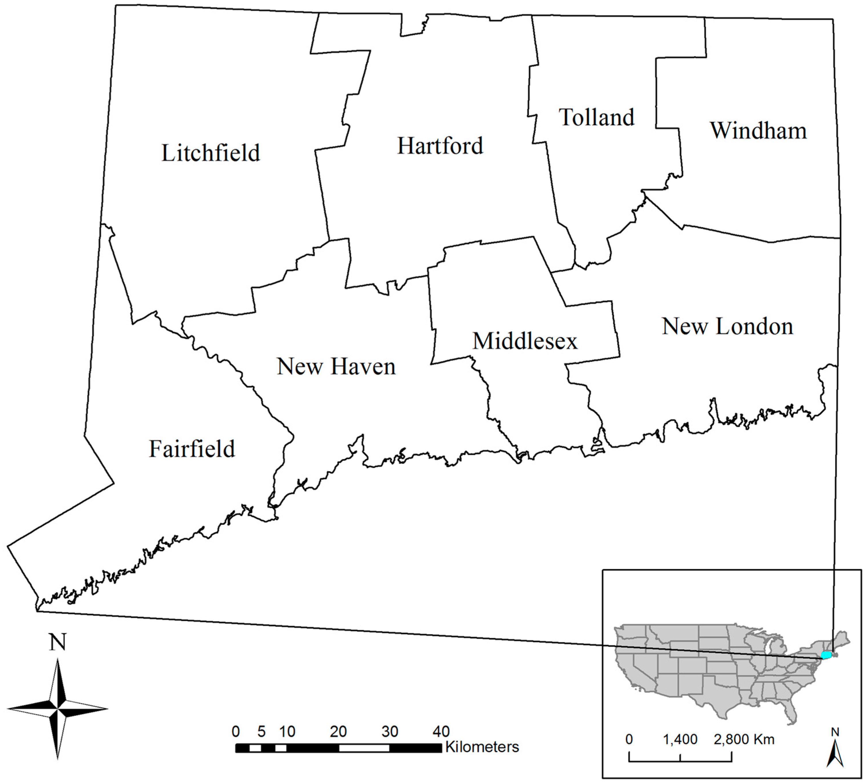
Connecticut is the third smallest state by area, but also the fourth most densely populated state among the 50 United States [23]. Land in Connecticut has gone through a tremendous change over the past two centuries. For example, up to 90% of the forest land was cleared for farming by the mid-1800s [24]. As farms were abandoned, most of the lands reverted back to mixed hardwood forests. Over the past fifty years, the region has undergone significant land use changes as housing and industrial development has encroached upon formerly rural and forested lands [18,25]. There are a few of studies that investigate how land uses and covers have changed throughout the Connecticut region. For example, Drummond and Loveland [26] studied land-use pressure and land transitions in the northeastern United States. Their results showed that a regional scale decline in forest cover was caused by contemporary land-use pressures in the eastern United States. Increasing crop production, pasturing, residential and industrial development, and uses of fuel wood and other resources caused nearly half or more of the natural forests to be cleared in the past three centuries.
Hurd et al. [27] analyzed forest fragmentation in the Salmon River watershed in Connecticut. They found that the interior forest area declined, while edge, transitional and perforated forest and urban areas increased between 1985 and 1999 [27,28]. Parent et al. [29] also studied the Salmon River watershed and found that the forest fragmentation in the region was mostly the result of land cover changes associated with building construction. They indicated that suburban development was a major contributor to forest fragmentation in the northeastern United States. Road development and socio-economic data were not taken into consideration in the study, however. It is also worth noting that the Center for Land Use Education And Research (CLEAR) at the University of Connecticut developed a temporal series of basic land cover information for the Thames watershed and surrounding towns to help gain a better understanding of the extent of land cover changes occurring in the Connecticut landscape [28].
Although the general picture of land use change in the past two centuries in Connecticut is known, prediction of future land use in the region remains difficult. And there is little research to predict the future land use change in this region. Complicating the prediction further, land use changes are not simple processes. It is difficult to conduct an accurate prediction of land use changes for a region without sufficient data and knowledge about the study area and well-developed and theoretically-informed models [30,31,32,33]. The models should have the ability to represent dynamically the processes of land-use change and biophysical processes. This has to be based on dynamic system models, which represent functional complexity [34]. In addition, future predictions of invasive plant distributions in the region have not incorporated land use change despite its importance [16,19,23,35] due to lack of future land use change data.
In this study, we aim to fill the data gap of future land use change predictions by: (1) explaining land use changes in Connecticut over 1996–2006; (2) constructing a Multi-layer Perceptron_Markov Chain (MLP_MC) model to predict short-term (12 years) changes in land use; and (3) investigate how short-term land use changes may affect landscape scale Japanese barberry invasion probability. The land use models provide a unique perspective into the drivers of land use change in our study region, while the short-term future land use predictions provide an insight into possible changes related to an important regional invasive plant.

2. Data and Methods

2.1. Study Area

The study area (Figure 1) includes the entire state of Connecticut (40°58′ N to 42°03′ N, 71°47′ W to 73°44′ W), a 14,357 km2 area in the northeastern United States. The elevations in Connecticut range from 0 to 2379 m, with a mean of 150 m. Connecticut has experienced a considerable population growth since 1950, which greatly affected the rate of urban sprawl in the area. The urban population has accounted for 78.5% of the total population before 1980 in Connecticut, but now accounts for 88.0%. The total population of Connecticut, about 3.3 million in 1990, has grown to over 3.5 million [36]. Approximately 400,000 acres of the forests have been removed since 1970. Since the 1990s, the major reason for the loss of forest has been land clearing for development in the State [37].

2.2. Data Preparation

A thematically-consistent land use/land cover (LULC) dataset for the years 1996, 2001, and 2006 was created using post-classification processing of national and regional LULC maps. These data were derived from the analysis of multiple dates of remotely sensed Landsat imagery [22] and were obtained from the Coastal Change Analysis Program (C-CAP) for 1996, 2001, and 2006 [38]. The details of C-CAP data can be found in the NOAA website [39]. Because the classification algorithms and schema were not identical for these data, we followed a three-steps procedure to standardize the data for our analysis. We classified the data into land use types that are related to invasive species studies/models. Beginning with the C-CAP data, we reclassified the previous LULC classes into 12 classes, including built-up area, urban grassland, pasture (including pasture land and wild grassland), cropland, shrub land (including scrub and shrub land), deciduous forest, evergreen forest, mixed forest, water body, emergent wetland, woody wetland, and barren land (Table 1). We used the National Land Cover Database (NLCD) 1992–2001 Retrofit Land Cover Change Product [40] to adjust the built-up areas in our dataset. Once all reclassifications and adjustments based on the NLCD 1992–2001 Retrofit Land Cover Change Product were performed, we used the 2006 map to disallow transitions from built-up areas to vegetated classes (a conversion that is unlikely, possibly due to LULC misclassification [41]). The final maps (Figure 2) retain the original 30 m × 30 m pixel resolution [22].

2.3. Selection of Drivers

The drivers of change were used to help understand what factors are the major contributors to LULC changes in the study area and predict those changes more accurately. The selection of the input variables is also important for predicting future LULC maps. In this study, spatial variables were considered based on previous research, team knowledge of the study area, and the availability of reliable data. Static spatial variables included elevation and slope, which express the suitability of locations for the land use/cover transitions under consideration. Elevation and slope can be useful biophysical variables for predicting deforestation in a rural context [42,43]. Topography often has effects on the spread and extent of forest conversion. For example, Sader and Joyce [44] found that deforestation decreases with the increase of slope gradient [45]. Elevation and slope (Figure 3) were generated from the earth digital elevation models (DEM) obtained from U.S. Geological Survey (USGS) [46].
Dynamic spatial variables for this study include the distance to the nearest road (DTR), the distance to the nearest built-up area (DTB), the distance to the nearest water body (DTW), the distance to the nearest cropland (DTC), the distance to the nearest pasture land (DTP) and population, which were calculated for different years. DTR was measured as the shortest Euclidian distance from each pixel to the nearest road, and other distances were calculated similarly. These variables were often used in land-use change models. Population has positive or negative relationships with LULC change, which has been proved in many studies [28,47]. Population maps of 1996, 2001, and 2006 were obtained from the U.S. Census Department and Connecticut Department of Public Health. The road system map for the year 2000 was obtained from U.S. Census Department. The Euclidian distance from a location to the nearest road was calculated using the road network data of Connecticut (Figure 4).
DTR is an important factor for deforestation and urban sprawl. It has been used in many studies to predict future LULC distributions. For example, Tyrrell et al. [28] and Araya and Cabral [47] both used DTR in their studies, showing a strong relationship between DTR and LULC change. In addition to road access, LULC change also depends on the types of LULC in the neighborhood. For instance, Khoi et al. [45] indicated that the location of water has effects on the location of cultivation, which means that DTW has a strong relationship with deforestation. Moreover, we also considered DTC and DTP. Tyrrell et al. [28] found that the distance to the nearest agricultural land is an important cause of forestland loss. Plans of conservation and development (COPDs) (2013–2018) were also considered as static spatial variables in this study. For example, lands that have some forms of restriction on development (such as permanently protected open spaces or properties where development rights have been acquired by governments (Office of Policy and Management in Connecticut), should not be changed. The protected areas (Figure 5) were treated as absolute constraints with a value of 0. The areas with a value of 1 are unconstrained and consequently are not impacted by conservation plans. All input data were resampled to the 30 m resolution with a processing extent of 6157 × 5138 pixels for modeling. The geomorphological maps were rasterized with continuous values.
The Cramer’s V coefficient (CVC) was used to quantify the associations between LULC classes and driving factors. The CVC value was calculated using the following equation [48]:
V = φ 2 min ( k 1 ,   r 1 ) = χ 2 / n min ( k 1 ,   r 1 ) ,
where φ is the coefficient of contingency, χ is derived from Pearson’s chi-squared test, n is the grand total of observations and k is the number of columns and r is the number of rows in the LULC images. CVC has a value between 0 and 1 (inclusive), and a value close to 1 indicates that a driving factor has a high potential of being an explanatory variable. The Multi-layer Perceptron (MLP) method was used to correlate predictor variables and LULC data in this study. The advantage of MLP is its capability for modeling complex non-linear relationships between variables [49].

2.4. MLP_Markov Chain Model (MLP_MC)

The MLP method is a type of artificial neural network (ANN) methods. Such methods are among the most widely used methods for modeling complex behaviors and patterns [50,51,52]. As a non-parametric technique, MLP has advantages in modeling complicated functional associations of land use classes. Compared with other models (e.g., the Weights of Evidence method), MLP is more appropriate for predicting future LULC change, since neural network outputs are able to express the change of various land cover types more adequately than individual probabilities obtained through the Weights of Evidence method [39]. Moreover, the nonlinear relationships between LULC change and its driving factors, such as population growth, policies and socio-economic variables, can be addressed smoothly by the MLP modeling framework. The MLP has been used in some studies to support binary and multiclass LULC change simulations [50,53,54,55]. The MLP model has the proven advantage of dealing with non-linear relationships without requiring the transformation of variables [56]. Many studies have shown that the MLP model can perform better than logistic regression and other empirical models in land change modeling [45,56,57,58,59]. The MLP_MC model is an integration of the MLP with a Markov chain model, developed by Eastman [60] for spatiotemporal dynamic modeling. In the MLP_MC model, the MLP allows the integration of the driving factors of LULC change and the Markov chain model to control the temporal dynamics of LULC change.

2.5. Model Parameters

A Markov chain model was used to calculate the amounts of change that may occur to some selected locations in the future [60]. A landscape transition probability matrix can be calculated by analyzing two LULC maps from different dates. Two transition matrices for the period of 1996–2001 and 2001–2006 were calculated by using the LULC maps of 1996, 2001 and 2006 (Table 2 and Table 3). These matrices have the information of probability of conversion from each class to those of other classes. The transition matrix of 1996–2001 (Table 2) was used for predicting the LULC in 2006. This prediction was used for model validation. Because the State’s COPD (2013–2018) was published by its Office of Policy and Management and was used as one of the variables in the model, we decided to predict LULC in 2018. Therefore, the transition matrix of 2001–2006 (Table 3) was used for predicting the future LULC in 2018. Because the projected time period (2006–2018) was not a multiple of the calibration period, three transition matrices were generated by a power rule. The values at each cell in the transition probability matrices were then fed into a quadratic regression. Therefore, there is a separate regression for each cell. The unknown transition probabilities were then interpolated by using the regression [61,62]. We ultimately implemented the MLP_MC model within the Land Change Modeler available in IDRISI Selva software [60] to analyze and predict LULC changes in Connecticut.
To avoid oscillating weight changes, the momentum factor was defined. Therefore, the calculated weight changes would not always be the same. A high momentum parameter can also help to increase the convergence speed of the system. However, setting the momentum parameter too high can create a risk of overshooting the minimum of change values, which can cause the system to become unstable. The rate parameters that control the size of weights and bias were set by using a training algorithm. The learning rate and momentum of the training algorithm were set based on trials and experiences. Both values have a range between 0 and 1. These factors can be set dynamically during runtime. In the present study, the momentum factor for the MLP_MC model was set to 0.5 and a dynamic learning rate was used. The outputs of MLP (values between 0 and 1) were used to express the potential of change. MLP neural network analysis was used to determine the weights of the transitions that would be included in the matrix of Markov chain transition probabilities for future prediction [63].

2.6. Investigation on How Short-Term Land Use Changes May Affect Landscape Scale Japanese Barberry Invasion Probability

We focused on an abundant invasive shrub in Connecticut to investigate the effects of land use change on probability of presence. The projections were based on the previously published models of Berberis thunbergii (Japanese barberry) [64], a perennial shrub native to East Asia that was introduced as an ornamental species to the northeast in 1875 [1]. The model, constructed in a hierarchical Bayesian framework and focused on New England (Connecticut, Massachusetts, Rhode Island, Vermont, New Hampshire, and Maine), was based on georeferenced presence and absence observations and local-scale habitat data collected from 2003–2009 as part of the Invasive Plant Atlas of New England project [65], native range presence and absence data [66], regional climate from the WorldClim database (average 1950–2000) [67], and landscape-scale LULC (2006) [22,64]. We used the best fit model for Japanese barberry in Ibanez et al. [35], which included five climate variables, six LULC variables, and two habitat variables (percent canopy coverage and presence of the most suitable local habitat, deciduous forest) (Table 4). Since predictions were made at a 5-min scale (see below), we set the canopy closure variable to 37 (representing the regional average) and the local habitat (deciduous forest) variable to 1 (representing assumed availability of a suitable local habitat patch within each 5′ × 5′ grid cell) following Ibanez et al. [35]. We made predictions using the parameters in Table 4 for 2006 and 2018 independently, and using observed LULC data in 2006 and our LULC model predictions for 2018. The original model was a logistic regression, so we converted the output of the prediction for each grid cell to a probability using the equation P (presence) = 1/(1 + exp()), where X is the matrix of covariates (i.e., one observation of each covariate in Table 4 for each grid cell) and β is the vector of parameter estimates. We estimated changes in the predicted probability of presence of Japanese barberry as the difference P (presence) in 2018 − P (presence) in 2006. The changes in presence probability were driven by changes in the landscape-scale summaries of LULC, but not climate, since we assumed climate to remain relatively unchanged on a near-term, 12-year timescale.
The models used regional and landscape variables at a 5-min scale, so we summarized our 2006 and 2018 LULC data to that scale, as percentages of each 5-min grid cell covered by each LULC category using the Geospatial Modeling Environment [68]. The models also simplified the LULC classes, so we have reclassified our maps to the same scheme. We combined built-up area, urban grassland and barren land into developed area, deciduous forest and mixed forest into deciduous & mixed forest, and emergent wetland and woody wetland into wetland. We are able to leverage a sophisticated model for invasive species distributions in this way, and compare the model predictions—the probability of presence of Japanese barberry—for 2006 and 2018.

3. Results and Analyses

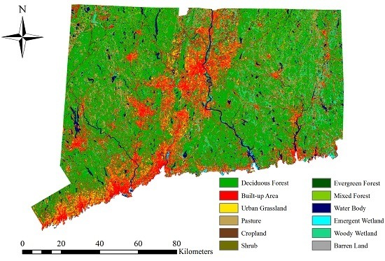
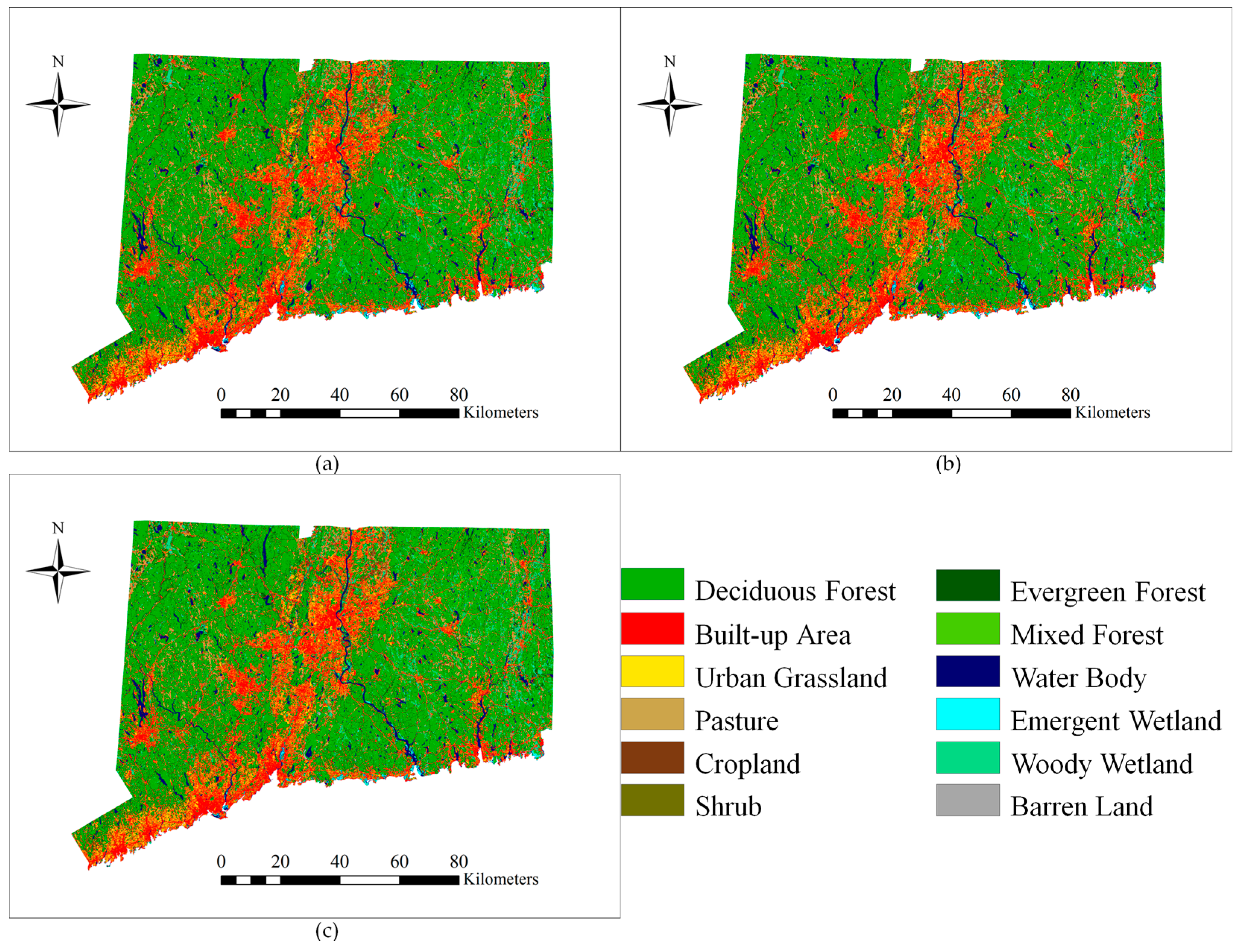
3.1. Observed LULC Changes

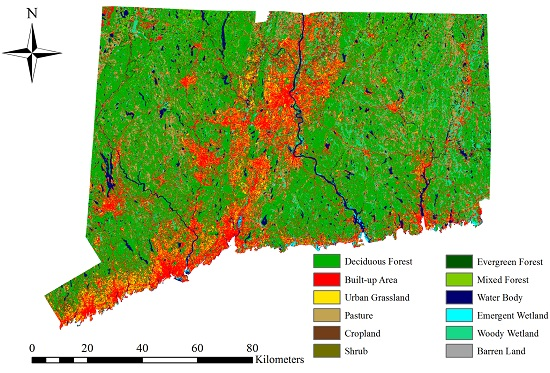
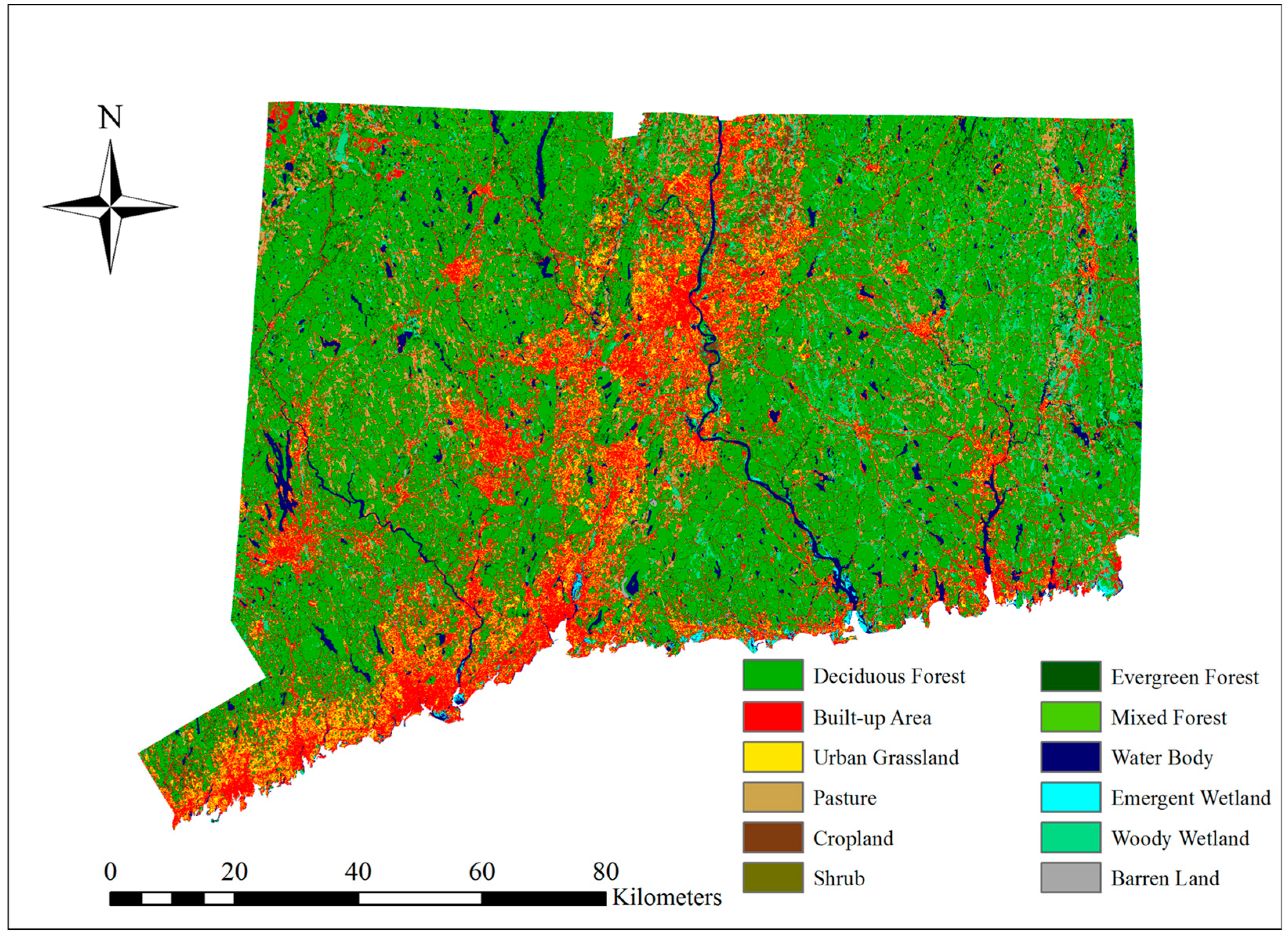
The results of LULC distribution for the years 1996, 2001 and 2006 show that deciduous forest was the dominant LULC class (from 48.04% to 47.67%) and the secondary class was built-up area (from 19.07% to 19.21%). There is a notable increasing trend for built-up area and agriculture classes, whereas a decreasing trend can be observed for forest classes (Table 5).
According to Table 6, the net deciduous forest loss for the period of 1996–2001 is 2289 ha. Drummond and Loveland [26] indicated that the largest contribution to forest expansion was the forest gain from grassland and shrub during the 1973–2000 period in the eastern United States. The situation, however, is different in Connecticut. A large portion of the deciduous forest loss was due to the transition of deciduous forest to shrub, which was 1242 ha, equivalent to 54.26% of the total deciduous forest loss. Shrub’s gain was also the result of the transition from evergreen forest to shrub (5.89%). The reader will recall that the “succession” process occurs when cleared areas transit naturally from grassland to shrub and then to forests. The gain of forest from scrub/shrub is small relative to its loss to other LULC classes, and it is possible that some deforested areas were classified into shrub. After a longer period, the areas will go through enough succession to become forest again.
The transition of shrub to forest should be observed in the next period (Table 7). The transition from deciduous forest to agriculture land (including cropland and pasture) was the second largest change, which was 527 ha, equivalent to 23.02% of the total deciduous forest loss. The third was the conversion of deciduous forest into built-up area, that is 229 ha and equivalent to 10% of the total deciduous loss. The shrub class increased by 1262 ha in total for this period, and the pasture class increased by 331 ha in total, which was mostly from deciduous forest. In some places, however, pasture was converted into built-up area (38 ha), cropland (36 ha) and urban grassland (31 ha). Alig et al. [69] and Tyrrell et al. [28] indicated that some pasture lands were relinquished to reforestation and frequently to development in the Northeastern United States, following the decline of the dairy industry. The situation was similar in Connecticut, but pasture lands were more likely to be converted into built-up area and cropland instead of forest. Cropland increased by 169 ha in total, which was mostly from deciduous forest. In some places, however, cropland was converted into barren land (22 ha) and built-up area (7 ha).
For the period 2001–2006, the net deciduous forest loss was 2505 ha. Most of the deciduous forest was lost to built-up area, which was 1206 ha, equivalent to 48.14% of the total deciduous loss. The transition of deciduous forest to agriculture land (including cropland and Pasture) was the second largest in area at 783 ha or equivalent to 31.26% of the total deciduous loss. Third was the conversion into urban grassland, accounting for 13.25% of the total deciduous loss. The built-up area increased by 1547 ha in total for this period, and most of the gain (77.76%) resulted from the conversion of deciduous forest. The urban grassland class increased by 408 ha, also gaining from deciduous forest. It was observed that urban and agricultural expansions were the main driving forces for the changes in forest because of increased population, residential development and proximity to rapidly developing area during this period. The pasture class increased by 601 ha, mostly from deciduous forest, evergreen forest and mixed forest. In some places, however, pasture was converted into shrub (71 ha), cropland (41 ha) and built-up area (33 ha). Similar to the LULC changes in the previous period, the loss of pasture land was related to the change in dairy production. Figure 6 shows how widespread the loss of deciduous forest from 1996 to 2006 was. The colored areas indicate where forest cover was lost.

3.2. Driving Factor Analysis

The overall CVC values are shown in Table 8. This index describes the quantitative levels of associations of a driving factor with individual or all LULC classes. The overall CVC value considers all variables together by Equation (1). It can help us understand how much a factor can influence LULC change. Normally, CVCs of about 0.15 or higher are considered important [
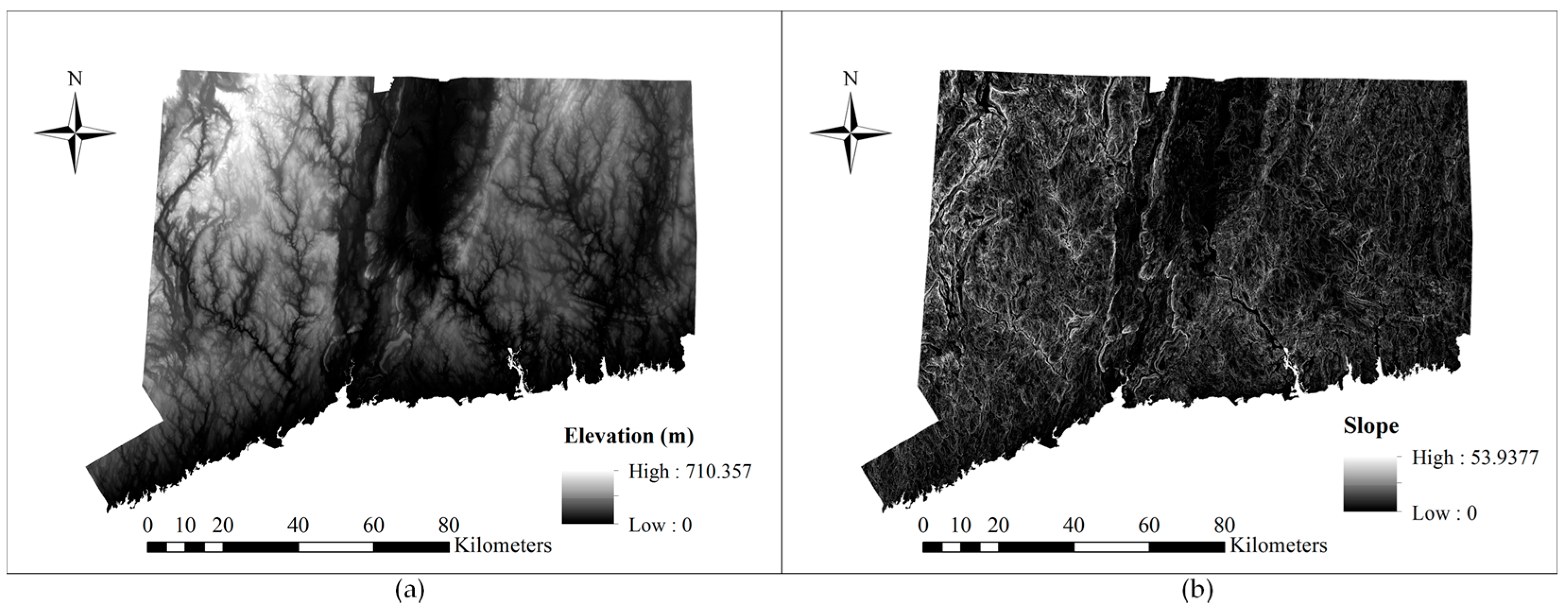
70]. Although some factors’ overall CVCs are slightly less than 0.15, the factors may still have relatively high values for specific LULC classes. For example, the overall CVC of elevation is 0.132, but CVCs of elevation with deciduous forest, urban grassland, built-up area, and water body are 0.306, 0.179, 0.170, and 0.156, respectively. This means that elevation has a relatively stronger relationship with the spread of deciduous forest. CVCs of slope with water, deciduous forest, and woody wetlands are 0.336, 0.307, and 0.158, respectively. Thus, slope appears to be a good predictor of water bodies and wetlands, because they are generally located in flat and lower areas. The results also indicate that slope has a similar influence on deciduous forest, as does elevation. Because of the small variation in topography and socioeconomic complexity, however, elevation and slope do not have large overall CVCs [71,72].
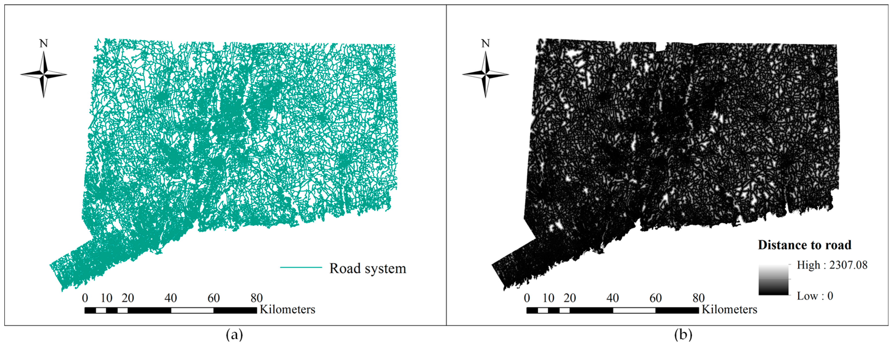
The DTR variable shows a good association with built-up area and deciduous forest, with CVCs of 0.483 and 0.356, respectively. Hence, it is one of the major drivers for forest change, because the development of new settlements tends to occur near existing settlements. CVCs of the DTC variable with cropland, pastures, and deciduous forest are 0.290, 0.176, and 0.142, respectively; and the CVCs of the DTP variable with pastures, deciduous forest, and built-up area are 0.501, 0.176, and 0.164, respectively. Both factors are useful in explaining the conversion of deciduous forest into agriculture. The CVC value of DTW with deciduous forest is 0.174, which indicates that the proximity to water has a relationship with forest change. CVCs of DTD with built-up area and urban grassland are 0.294 and 0.285, respectively, meaning that urban sprawl has a strong relationship with deforestation. The CVC of DTM with evergreen forest is 0.155. Similarly, the CVC of DTE with mixed forest is 0.154. Those two factors can partly explain the conversion between mixed forest and evergreen forest. CVCs of DTB with built-up area, deciduous forest, and urban grassland are 0.430, 0.380 and 0.266, respectively.
Apparently, the DTB plays an important role in LULC change in Connecticut, such as reduction in forest areas and increased new settlement areas. Not surprisingly, deforestation is stronger at places closer to an existing built-up area. And the areas closer to existing built-up areas have higher probabilities of conversion to built-up areas. CVC values of population with deciduous forest, urban grassland, and built-up area are 0.209, 0.205 and 0.197, respectively. These results indicate that population pressure should be an important driving force to the increase of the built-up area and conversion of forest to other land use classes.

3.3. Model Validation

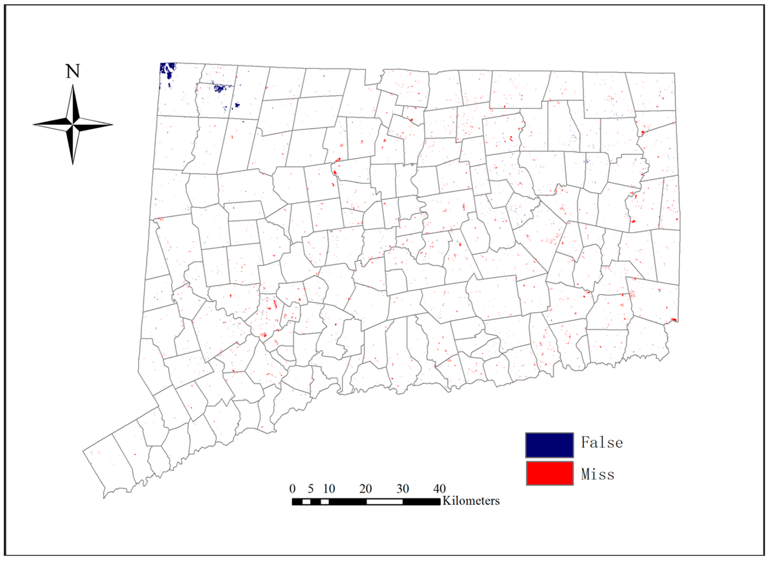
A predicted map for model validation was created for the year 2006 using the transition probability matrix estimated from the 1996 and 2001 LULC maps. This validation aimed to evaluate the quality of the predicted land use map in comparison with the real land use map. A three-way cross-tabulation between the real 2001 map, the real 2006 map, and the predicted 2006 map was conducted for the validation. By comparing the real 2001 LULC map with the real 2006 LULC map, the actual change locations can be discovered, and by comparing the real 2001 LULC map with the predicted 2006 LULC map, the predicted change locations can also be identified. Then, comparing the actual change locations with the predicted change locations can find out where the prediction errors are located. Figure 6 indicates that the LULC change model worked effectively because the predicted map and the real map for 2006 coincided in most places and only minor differences occurred. The difference map is shown in Figure 7.
IDRISI Selva [73] provides a Validation Module, which can measure the agreement between two categorical maps. Cohen’s kappa coefficient is a commonly used index, which measures inter-rater agreement for qualitative (categorical) items. Kappa is always less than or equal to 1. A value of 1 means perfect agreement. Pontius [74,75] suggested, however, that the standard Kappa coefficient cannot provide enough information because it does not have ability to distinguish the quantification error with the location error [74,75]. In order to solve this problem, two more kappa statistics are provided: Kappa for no information (Kno), and Kappa for grid-cell level location (Klocation). The Kno statistic is an improved general statistic over the traditional Kappa Index of Agreement (Kstandard), as it penalizes large quantity errors and rewards correct location classifications. Klocation indicates how well the grid cells are located on the landscape. In order to calculate those Kappa statistics, the real 2006 LULC map and the predicted 2006 LULC map were used as the reference map and the comparison map, respectively. Furthermore, five statistics were calculated to indicate how well the comparison map agrees with the reference map [67,68]: agreement due to chance (AgreementChance), agreement due to quantity (AgreementQuantity), agreement due to location at the grid cell level (AgreementGridcell), disagreement due to location at the grid cell level (DisagreeGridcell), and disagreement due to quantity (DisagreeQuantity) (Table 9).
The results in Table 9 indicate that the MLP_MC model has a very high capability to predict future LULC changes. It is also important to note that the DisagreeGridcell and DisagreeQuantity indices can help us understand the predicted results. In Table 9, the DisagreeGridcell is larger than the DisagreeQuantity. This means that the model has a higher ability to predict the LULC changes in quantity than in location in the study area. To reduce the DisagreeGridcell value, more explanatory variables about location should be considered in further studies.

3.4. Change Predictions

The LULC map for the year 2018 (Figure 8) was predicted using the LULC maps of 2001 and 2006. The results of a predicted LULC scenario (Figure 9) show an obvious increase in developed area (built-up area and urban grassland) and agriculture land (cropland and pasture). In addition, it shows a drastic decrease in forest area (deciduous, mixed, and evergreen forest). The model predicts that the study area will lose 5535 ha deciduous forest and gain 3502 ha in built-up area from 2006 to 2018. The conversion of deciduous forest into built-up area is predicted to be 2884 ha in the 12 years by 2018, accounting for 52.10% of the total deciduous forest loss. Urban growth will continue in the future, but the rate of deforestation will slow down. Because of an increasing demand for agriculture area driven by population pressure, pasture and cropland will increase by 2325 ha and 253 ha, respectively. The conversion of deciduous forest into agriculture land is predicted to be 1903 ha by 2018, equivalent to 34.38% of the total deciduous forest loss. In addition, areas near the built-up area and agriculture land appear to be vulnerable to conversion. These areas may need more protection measures if the total forest area is to be maintained in the future. Mature forest stands are necessary to maintain a diversity of wildlife and native plants.

3.5. Landscape Scale Japanese Barberry Invasion Probability Affected by Short-Term Land Use Changes

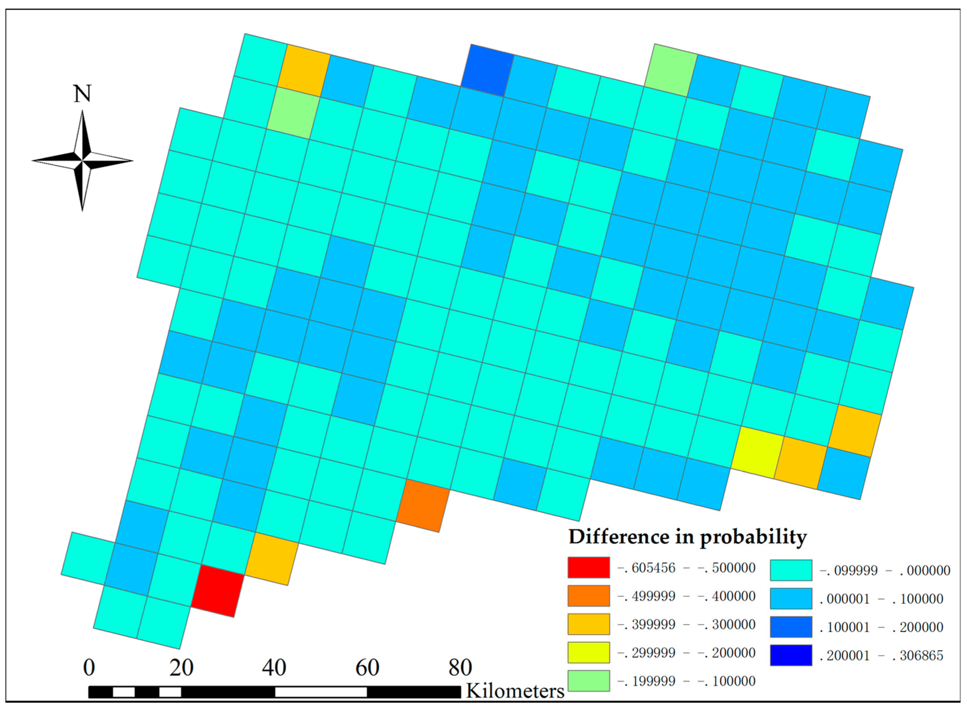
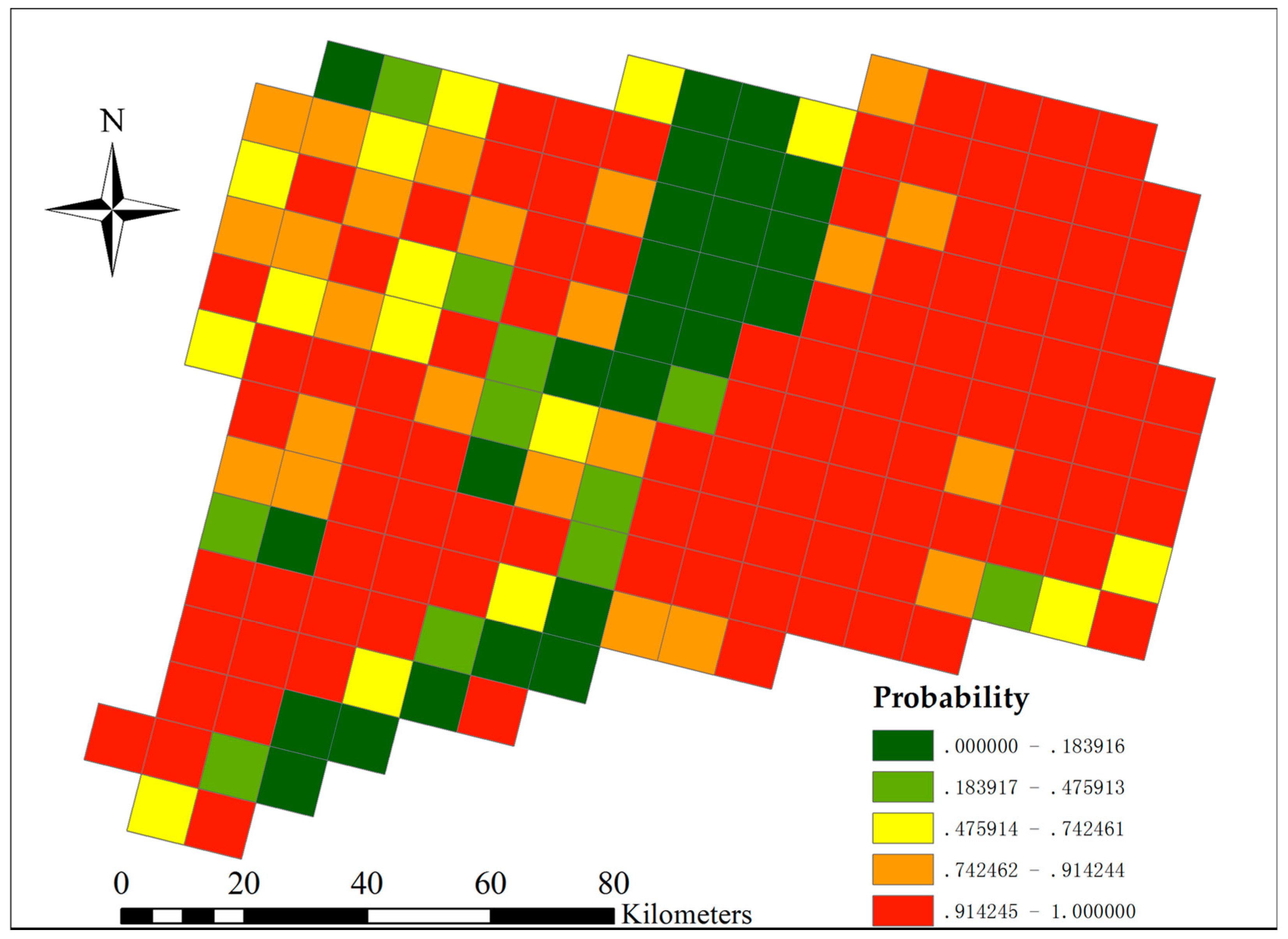
The projected LULC changes by 2018 yielded subtle, but measurable changes in the predicted probability of Japanese barberry. The northwest and south-central areas of the state had slightly reduced probabilities of barberry presence, whereas the north-central and northeast areas of the state had slightly higher risk with projected LULC change (Figure 10). The probability change for each grid cell was generally 0.1 more or less than the 2006 baseline estimate, with only about 6% of the cells falling outside of that range. The changes in invasion risk do not negate the overall risk, however; areas that had high probability of presence (e.g., most areas except the Connecticut River Valley) in 2006 continue to be at high risk in the future (Figure 11). Landscape-scale loss in the percentage of deciduous and mixed forest cover was significantly correlated with decreased invasion risk for this species (r = 0.16, p = 0.03) and gain in developed cover was correlated with increased risk (r = 0.64, p < 0.0001).

4. Discussions

Changes in LULC will influence forest distribution in the study area. Since urbanization can increase local temperature (e.g., the urban heat island effect), human activities, and damage to the natural environment, it is possible to see a shift in species composition between urban and rural areas. Human activities in urban areas also change the characteristics of soils. For example, soils in urban areas have higher concentrations of heavy metals and organic matter than in rural areas. For some species, this kind of change could reduce habitat suitability. Moreover, forests adjacent to residential areas tend to have a higher number of invasive species compared to those surrounded by industrial lands.
In the Northeast, dairy production was dominated by small dairies, which disappeared rapidly because of increasing mechanization and industry competition [76]. Therefore, decreasing dairy production led to pasture’s natural conversion to shrub. Cropland increased by 217 ha in total, mostly converted from deciduous forest and pasture. Rapidly increasing population brought the pressure to existing agriculture land by replacing forest.
Forest utilization, such as timber harvesting, extraction of non-timber products, construction of logging and transport roads and facilities for logging camps, and conversion of natural forest to plantations, may have direct and indirect negative impacts on forest biodiversity by promoting the invasion of alien species. Some studies have shown that forest fragmentation may accelerate the spread of invasive species [32,36]. Simply, a high proportion of evergreen forest in a landscape tends to deter invasive plants [20,64]. But the portion of evergreen forest area is relatively low in Connecticut; and based on our prediction, some evergreen forest is expected to be lost (272 ha) by 2018. Therefore, to stem the spread of invasive plants, it would make sense for policy makers to take actions to preserve evergreen forest in the region.
Moreover, road systems provide essential access to forests for timber extraction. A good road system is an important requirement for sustainable forest management. But without quality design and maintenance, roads are often the cause of a variety of environmental problems associated with forest harvesting operations [77]. In some situations, roads may also initiate or accelerate the invasion of non-native species that ultimately displace native species. Additionally, the increased level of human activities in previously inaccessible areas (activities that are facilitated by roads) can cause environmental problems, including the possible introduction of alien species [78]. Mosher et al. [18] indicated that the greatest incidence of invasion is in post-agricultural settings, e.g., fields that are currently abandoned or have reverted to forest. Our study shows that portions of the pasture land and cropland were converted to urban grassland during 1996 to 2006 in Connecticut, which might increase the current and future richness of invasive species.

5. Conclusions

In this study, LULC change in Connecticut from 1996 to 2006 was analyzed and LULC change from 2006 to 2018 was predicted using the MLP_MC model. In addition, the effect of LULC change on the invasion risk of an abundant invasive shrub, Japanese barberry, was studied. The results show that the total area of forests, especially deciduous forest, has been decreasing. That decrease is primarily caused by urban development and other human activity in the study area. We also found that forest areas near built-up areas and agriculture lands appear to be more vulnerable to conversion. These predicted LULC changes translated into subtle changes in the invasion risk by the invasive shrub Japanese barberry. While the magnitude of change in Japanese barberry risk was low over this relatively short time-scale, it could be compounded by longer-term changes in LULC and changes in climate. Future work should focus on these interacting global change factors and the generalization of their effects on invasive plants in the region and beyond.
In summary, this study provides reliable LULC data, which is useful for the study of invasive species in the Connecticut region. The information is also useful for early detection and in the future refinement of conservation policy aimed at reducing the spread of invasive species. Our findings suggest that forest conversion should be controlled and managed in service of invasive species control. In addition, our research indicates that the MLP_MC model can predict future LULC with a reasonable accuracy. Nevertheless, it is important to note that predicting the actual location of LULC change is challenging. Explanatory variables about locations are usually not sufficient and important social economical drivers vary with time. Future work will consider dealing with these limitations.

Acknowledgments

This research is partially supported by USA NSF grant No. 1414108. Authors have the sole responsibility to all of the viewpoints presented in the paper. The publication cost is supported by USA NSF grant No. 1414108.

Author Contributions

Wenjie Wang, Chuanrong Zhang, Jenica M. Allen, Weidong Li, Mark A. Boyer, Kathleen Segerson and John A. Silander, Jr. contributed to the research design. Wenjie Wang, Chuanrong Zhang, Jenica M. Allen and Weidong Li contributed to the writing of the paper. Wenjie Wang and Jenica M. Allen undertook analysis of datasets. Wenjie Wang, Chuanrong Zhang, Jenica M. Allen, Weidong Li, Mark A. Boyer, Kathleen Segerson and John A. Silander, Jr. contributed to the revisions, and critical reviews from the draft to the final stages of the paper.

Conflicts of Interest

The authors declare no conflict of interest.

Abbreviations

The following abbreviations are used in this manuscript:
LULCLand use and land cover
MLPMulti-Layer Perceptron
MLP_MCMulti-Layer Perceptron Markov Chain
NLCDNational Land Cover Database
DEMDigital elevation models
DTRThe distance to the nearest road
DTBThe distance to the nearest built-up area
DTWThe distance to the nearest water body
DTCThe distance to the nearest cropland
DTPThe distance to the nearest pasture land
CVCCramer’s V coefficient
KnoKappa for no information
KlocationKappa for grid-cell level location
Kstandard
AgreementChance
Kappa Index of Agreement
Agreement due to chance
AgreementQuantityAgreement due to quantity
AgreementGridcellAgreement due to location at the grid cell level
DisagreeGridcellDisagreement due to location at the grid cell level
DisagreeQuantityDisagreement due to quantity

References

  1. Mehrhoff, L.J.; Silander, J.A., Jr.; Leicht, S.A.; Mosher, E.S.; Tabak, N.M. Invasive Plant Atlas of New England. 2003. Available online: http://www.eddmaps.org/ipane/ (accessed on 20 November 2015).
  2. Ehrenfeld, J.G. Ecosystem consequences of biological invasions. Annu. Rev. Ecol. Evol. Syst. 2010, 41, 59–80. [Google Scholar] [CrossRef]
  3. Mehrhoff, L.J. Immigration and expansion of the New England Flora. Rhodora 2000, 102, 280–298. [Google Scholar]
  4. Silander, J.A.; Ibáñez, I.; Mehrhoff, L.J. The biology and ecology of invasive species—The importance of international collaboration in predicting the spread of invasive species. In Proceedings of the NIAES International Symposium, Tsukuba, Japan, 22–23 October 2007.
  5. Pimentel, D.; Zuniga, R.; Morrison, D. Update on the environmental and economic costs associated with alien-invasive species in the United States. Ecol. Econom. 2005, 52, 273–288. [Google Scholar] [CrossRef]
  6. Olson, L.J. The economics of terrestrial invasive species: A review of the literature. Agr. Resour. Econ. Rev. 2006, 35, 178–194. [Google Scholar]
  7. Farnsworth, E.J. Patterns of plant invasions at sites with rare plant species throughout New England. Rhodora 2004, 106, 97–117. [Google Scholar]
  8. Barton, A.M.; Brewster, L.B.; Cox, A.N.; Prentiss, N.K. Non-indigenous woody invasive plants in a rural New England town. Biol. Invasions 2004, 6, 205–211. [Google Scholar] [CrossRef]
  9. Wang, H.-H. Occupation, Dispersal, and Economic Impact of Major Invasive Plant Species in Southern U.S. Forests. Ph.D. Thesis, Texas A&M University, College Station, TX, USA, 2009. [Google Scholar]
  10. Duik-Wasser, M.A.; Vourc’h, G.; Cislo, P.; Hoen, A.G.; Melton, F.; Hamer, S.A.; Rowland, M.; Cortinas, R.; Hickling, G.J.; Tsao, J.I.; et al. Field and climate-based model for predicting the density of host-seeking nymphal Ixodes scapularis, an important vector of tick-borne disease agents in the eastern United States. Glob. Ecol. Biogeogr. 2010, 19, 504–514. [Google Scholar]
  11. Defenders of Wildlife. Available online: www.defenders.org/publications/connecticut.pdf (accessed on 20 November 2015).
  12. Williams, S.C.; Ward, J.S.; Worthley, T.E.; Stafford, K.C., III. Managing Japanese barberry (Ranunculales: Berberidaceae) infestations reduced blacklegged tick (Acari: Ixodidae) abundance and infection prevalence with Borrelia burgdorferi (Spirochaetales: Spirochaetaceae). Environ. Entomol. 2009, 38, 977–984. [Google Scholar] [CrossRef] [PubMed]
  13. Williams, C.S.; Ward, J.S. Effects of Japanese barberry (Ranunculales: Berberidaceae) removal and resulting microclimatic changes in Ixodes scapularus (Acari: Ixodidae) abundances in Connecticut, USA. Environ. Entomol. 2010, 39, 1911–1921. [Google Scholar] [CrossRef] [PubMed]
  14. Ehrenfeld, J.G.; Kourtev, P.; Huang, W. Changes in soil functions following invasions of exotic understory plants in deciduous forests. Ecol. Appl. 2001, 11, 1287–1300. [Google Scholar] [CrossRef]
  15. Vilá, M.; Ibáñez, I. Plant invasions in the landscape. Landsc. Ecol. 2011, 26, 461–472. [Google Scholar] [CrossRef]
  16. With, K.A. The landscape ecology of invasive spread. Conserv. Biol. 2002, 16, 1192–1203. [Google Scholar] [CrossRef]
  17. Degasperis, B.G.; Motzkin, G. Windows of opportunity: Historical and ecological controls on Berberis thunbergii invasions. Ecology 2007, 88, 3115–3125. [Google Scholar] [CrossRef] [PubMed]
  18. Mosher, E.S.; Silander, J.A., Jr.; Latimer, A.M. The role of land-use history in major invasions by woody plant species in the northeastern North American landscape. Biol. Invasions 2009, 11, 2317–2328. [Google Scholar] [CrossRef]
  19. Matlack, G.R.; Schaub, J.E. Long-term persistence and spatial assortment of nonnative plant species in deciduous forests of varying age. Ecography 2011, 34, 649–658. [Google Scholar] [CrossRef]
  20. Merow, C.; LaFleur, N.; Silander, J.; Wilson, A.; Rubega, M. Developing dynamic, mechanistic species distribution models: Predicting bird-mediated spread of invasive plants across northeastern North America. Am. Nat. 2011, 178, 30–43. [Google Scholar] [CrossRef] [PubMed]
  21. Álvarez-Berríos, N.L.; Redo, D.J.; Aide, T.M.; Clark, M.L.; Grau, R. Land change in the greater Antilles between 2001 and 2010. Land 2013, 2, 81–107. [Google Scholar] [CrossRef]
  22. Allen, J.M.; Leininger, T.J.; Hurd, J.D., Jr.; Civco, D.L.; Gelfand, A.E.; Silander, J.A., Jr. Socioeconomics drive woody invasive plant richness in New England, USA through forest fragmentation. Landsc. Ecol. 2013, 28, 1671–1686. [Google Scholar] [CrossRef]
  23. U.S. Census Bureau. American FactFinder. Available online: http://factfinder.census.gov/faces/tableservices/jsf/pages/productview.xhtml?pid=ACS_14_5YR_DP05&prodType=table (accessed on 18 November 2015).
  24. Foster, D.R.; Aber, J.D. Forests in Time: The Environmental Consequences of 1,000 Years of Change in New England; Yale University Press: New Haven, CT, USA, 2004. [Google Scholar]
  25. Foster, D.R.; Donahue, B.M.; Kittredge, D.B.; Lambert, K.F.; Hunter, M.L.; Hall, B.R.; Irland, L.C.; Lilieholm, R.J.; Orwig, D.A.; D’Amato, A.W.; et al. Wildlands and Woodlands: A vision for the New England landscape; Harvard Forest, Harvard University: Petersham, MA, USA, 2010. [Google Scholar]
  26. Drummond, M.A.; Loveland, T.R. Land-use pressure and a transition to forest-cover loss in the eastern United States. BioScience 2010, 60, 286–298. [Google Scholar] [CrossRef]
  27. Hurd, J.D.; Wilson, E.H.; Lammey, S.G.; Civco, D.L. Characterization of forest fragmentation and urban sprawl using time sequential Landsat imagery. In Proceedings of the ASPRS 2001 Annual Convention, St. Louis, MO, USA, 23–27 April 2001.
  28. Tyrrell, M.L.; Hall, M.H.P.; Sampson, R.N. Dynamics Models of Land-Use Change in Northeastern USA: Developing Tools, Techniques and Talents for Effective Conservation Action; GISF Research Paper 003; Yale University Global Institute of Sustainable Forestry: New Haven, CT, USA, 2004. [Google Scholar]
  29. Parent, J.; Civco, D.; Hurd, J. Simulating future forest fragmentation in a Connecticut region undergoing suburbanization. In Proceedings of the Annual Conference of ASPRS, Tampa, FL, USA, 7–11 May 2007.
  30. Pontius, R.G., Jr. Modeling Tropical Land Use Change and Assessing Policies to Reduce Carbon Dioxide Release from Africa. Ph.D. Thesis, State University of New York Col. of Environmental Science & Forestry, Syracuse, NY, USA, 1994. [Google Scholar]
  31. Lambin, E.F. Modelling Deforestation Processes: A Review; Report no. EUR-15744-EN; Office of Official Publications of the European Community: Luxembourg, 1994. [Google Scholar]
  32. Hochholzer, H. Connecticut‘s Forest Resource Assessment and Strategy 2010 Building a better tomorrow for Connecticut’s forests today. 2010. Available online: http://www.ct.gov/deep/lib/deep/forestry/assessment_and_strategy/assessment__strategy.pdf (accessed on 18 November 2015). [Google Scholar]
  33. Behera, S.; Ghanty, S.; Ahmad, F.; Santra, S.; Banerjee, S. UV-Visible spectrophotometric method development and validation of assay of paracetamol tablet formulation. J. Anal. Bioanal. Tech. 2012, 3, 151. [Google Scholar] [CrossRef]
  34. Veldkamp, A.; Lambin, E.F. Predicting land-use change. Agric. Ecosyst. Environ. 2001, 85, 1–6. [Google Scholar] [CrossRef]
  35. Ibáñez, I.; Clark, J.S.; Dietze, M.C. Estimating colonization potential of migrant tree species. Glob. Chang. Biol. 2009, 15, 1173–1188. [Google Scholar] [CrossRef]
  36. Division, U.S. Census Bureau Administration and Customer Services. U.S. Census Bureau Publications—Census of Population and Housing. Available online: http://www.census.gov/prod/www/decennial.html (accessed on 18 November 2015).
  37. Martin, C. The Economic Importance of Connecticut’s Forest Based Economy 2015; North East State Forester Association: Concord, NH, USA, 2015; p. 20. [Google Scholar]
  38. National Oceanic and Atmospheric Administration (NOAA). (1996, 2001, 2006) Coastal Change Analysis Program Land Cover. Available online: http://www.csc.noaa.gov/crs/lca/northeast.html (accessed on 10 January 2015).
  39. Coastal Change Analysis Program Regional Land Cover and Change. Available online: https://coast.noaa.gov/dataregistry/search/collection/info/ccapregional (accessed on 10 January 2015).
  40. Fry, J.A.; Coan, M.J.; Homer, C.G.; Meyer, D.K.; Wickham, J.D. Completion of the National Land Cover Database (NLCD) 1992–2001 Land Cover Change Retrofit Product; U.S. Geological Survey Open-File Report 2008-1379; U.S. Geological Survey: Arcata, CA, USA, 2009.
  41. Clark, M.L.; Aide, T.M.; Grau, H.R.; Riner, G. A scalable approach to mapping annual land cover at 250 m using MODIS time series data: A case study in the dry Chaco ecoregion of South America. Remote Sens. Environ. 2010, 114, 2816–2832. [Google Scholar] [CrossRef]
  42. Kim, I.; Le, Q.B.; Park, S.J.; Tenhunen, J.; Koeller, T. Driving forces in archetypical land-use changes in a mountainous watershed in east Asia. Land 2014, 3, 957–980. [Google Scholar] [CrossRef]
  43. Lambin, E.F. Modelling and monitoring land-cover change processes in tropical regions. Prog. Phys. Geogr. 1997, 21, 375–393. [Google Scholar] [CrossRef]
  44. Sader, S.A.; Joyce, A.T. Deforestation rates and trends in Costa Rica, 1940–1983. Biotropica 1988, 20, 11–19. [Google Scholar] [CrossRef]
  45. Khoi, D.D.; Murayama, Y. Forecasting areas vulnerable to forest conversion in the Tam Dao national park region, Vietnam. Remote Sens. 2010, 2, 1249–1272. [Google Scholar] [CrossRef]
  46. U.S. Geological Survey (USGS). National Land Cover Dataset. 1992. Available online: http://seamless.usgs.gov/index.php (accessed on 10 January 2015). [Google Scholar]
  47. Araya, Y.H.; Cabral, P. Analysis and modeling of urban land cover change in Setúbal and Sesimbra, Portugal. Remote Sens. 2010, 2, 1549–1563. [Google Scholar] [CrossRef]
  48. Liebetrau, A.M. Measures of Association; Quantitative Applications in the Social Sciences Series; Sage Publications: Newbury Park, CA, USA, 1983; Volume 32, pp. 15–16. [Google Scholar]
  49. Pérez-Vega, A.; Mas, J.-F.; Ligmann-Zielinska, A. Comparing two approaches to land use/cover change modeling and their implications for the assessment of biodiversity loss in a deciduous tropical forest. Environ. Model. Softw. 2012, 29, 11–23. [Google Scholar] [CrossRef]
  50. Pijanowski, B.C.; Brown, D.G.; Shellito, B.A.; Manik, G.A. Using neural networks and GIS to forecast land use changes: A Land Transformation Model. Comput. Environ. Urban Syst. 2002, 26, 553–575. [Google Scholar] [CrossRef]
  51. Thapaa, R.B.; Murayamab, Y. Scenario based urban growth allocation in Kathmandu Valley, Nepal. Landsc. Urban Plan. 2012, 105, 140–148. [Google Scholar] [CrossRef]
  52. Pijanowski, B.C.; Tayyebi, A.; Doucette, J.; Pekin, B.K.; Braun, D.; Plourde, J. A big data urban growth simulation at a national scale: Configuring the GIS and neural network based Land Transformation Model to run in a High Performance Computing (HPC) environment. Environ. Model. Softw. 2014, 51, 250–268. [Google Scholar] [CrossRef]
  53. Almeida, C.M.; Gleriani, J.M.; Castejon, E.F.; Soares-Filho, B.S. Using neural networks and cellular automata for modelling intra-urban land-use dynamics. Int. J. Geogr. Inf. Sci. 2008, 22, 943–963. [Google Scholar] [CrossRef]
  54. Lin, Y.-P.; Chu, H.-J.; Wu, C.-F.; Verburg, P.H. Predictive ability of logistic regression, auto-logistic regression and neural network models in empirical land-use change modeling—A case study. Int. J. Geogr. Inf. Sci. 2011, 25, 65–87. [Google Scholar] [CrossRef] [Green Version]
  55. Shafizadeh-Moghadam, H.; Hagenauer, J.; Farajzadeh, M.; Helbich, M. Performance analysis of radial basis function networks and multilayer perceptron networks in modeling urban change: A case study. Int. J. Geogr. Inf. Sci. 2015, 29, 606–623. [Google Scholar] [CrossRef]
  56. Lek, S.; Delacoste, M.; Baran, P.; Dimopoulos, I.; Lauga, J.; Aulanier, S. Application of neural networks to modelling non-linear relationships in ecology. Ecol. Model. 1996, 90, 39–52. [Google Scholar] [CrossRef]
  57. Zhou, J.; Civco, D. Using genetic learning neural networks for spatial decision making in GIS. Photogramm. Eng. Remote Sens. 1996, 62, 1287–1295. [Google Scholar]
  58. Mas, J.F.; Puig, H.; Palacio, J.L.; Lopez, A.S. Modelling deforestation using GIS and artificial neural networks. Environ. Model. Softw. 2004, 19, 461–471. [Google Scholar] [CrossRef]
  59. Yuan, H.; Van Der Wiele, C.F.; Khorram, S. An automated artificial neural network system for land use/land cover classification from Landsat TM imagery. Remote Sens. 2009, 1, 243–265. [Google Scholar] [CrossRef]
  60. Eastman, J.R. IDRISI Taiga, Guide to GIS and Remote Processing; Clark University: Worcester, MA, USA, 2009. [Google Scholar]
  61. Takada, T.; Miyamoto, A.; Hasegawa, S.F. Derivation of a yearly transition probability matrix for land-use dynamics and its applications. Landsc. Ecol. 2010, 25, 561–572. [Google Scholar] [CrossRef]
  62. Mas, J.F.; Kolb, M.; Paegelow, M.; Olmedo, M.T.C.; Houet, T. Inductive pattern-based land use/cover change models: A comparison of four software packages. Environ. Model. Softw. 2014, 51, 94–111. [Google Scholar] [CrossRef] [Green Version]
  63. Ahmed, B.; Ahmed, R. Modeling urban land cover growth dynamics using multi-temporal satellite images: A case study of Dhaka, Bangladesh. ISPRS Int. J. Geo-Inf. 2012, 1, 3–31. [Google Scholar] [CrossRef]
  64. Ibanez, I.; Silander, J.A., Jr.; Wilson, A.; LaFleur, N.; Tanaka, N.; Tsuyama, I. Multi-variate forecasts of potential distribution of invasive plant species. Ecol. Appl. 2009, 19, 359–375. [Google Scholar] [CrossRef] [PubMed]
  65. Bois, S.T.; Silander, J.A., Jr.; Mehrhoff, L.J. Invasive Plant Atlas of New England: the role of citizens in the science of invasive alien species detection. BioScience 2011, 61, 763–770. [Google Scholar] [CrossRef]
  66. Tanaka, N. PRDB: Phytosociological Relevé Database. Forestry and Forest Products Research Institute: Tsukuba, Ibaraki, Japan, 2007. Available online: http://www.ffpri.affrc.go.jp/labs/prdb/index.html (accessed on 20 November 2015). [Google Scholar]
  67. Hijmans, R.J.; Cameron, S.E.; Parra, J.L.; Jones, P.G.; Jarvis, A. Very high resolution interpolated climate surfaces for global land areas. Int. J. Climatol. 2005, 25, 1965–1978. [Google Scholar] [CrossRef]
  68. Geospatial Modelling Environment. Available online: http://www.spatialecology.com/gme/index.htm (accessed on 20 November 2015).
  69. Alig, R.; Mills, J.; Butler, B. Private timberlands: Growing demands, shrinking land base. J. For. 2002, 100, 32–37. [Google Scholar]
  70. Eastman, J.R. IDRISI Selva Tutorial; IDRISI Production; Clark Labs-Clark University: Worcester, OH, USA, 2012. [Google Scholar]
  71. Deep, S.; Saklani, A. Urban sprawl modeling using cellular automata. Egypt. J. Remote Sens. Space Sci. 2014, 17, 179–187. [Google Scholar] [CrossRef]
  72. Pontius, R.G., Jr. Land-cover change model validation by an ROC method for the Ipswich watershed, Massachusetts, USA. Agric. Ecosyst. Environ. 2001, 85, 239–248. [Google Scholar] [CrossRef]
  73. IDRISI Selva 17.02. Clark Labs, Clark University, 2015. Available online: https://clarklabs.org/downloads/ (accessed on 22 August 2015).
  74. Pontius, R.G., Jr. Quantification error versus location error in the comparison of categorical maps. Photogramm. Eng. Remote Sens. 2000, 66, 1011–1016. [Google Scholar]
  75. Pontius, R.G., Jr. Statistical methods to partition effects of quantity and location during comparison of categorical maps at multiple resolution. Photogramm. Eng. Remote Sens. 2002, 68, 1041–1049. [Google Scholar]
  76. MacDonald, J.M.; O’Donoghue, E.J.; McBride, W.D.; Nehring, R.F.; Sandretto, C.L.; Mosheim, R. Profits, Costs, and the Changing Structure of Dairy Farming; Economic Research Report ERR-47; U.S. Department of Agriculture: Naches, WA, USA, 2007.
  77. La Mela Veca, D.S.; Cullotta, S.; Sferlazza, S.; Maetzke, F.G. Anthropogenic influences in land use/land cover changes in Mediterranean forest landscapes in Sicily. Land 2016, 5, 3. [Google Scholar] [CrossRef] [Green Version]
  78. Mortensen, D.A.; Rauschert, E.S.J.; Nord, A.N.; Jones, B.P. Forest roads facilitate the spread of invasive plants. Invasive Plant Sci. Manag. 2009, 2, 191–199. [Google Scholar] [CrossRef]
Figure 1. The state of Connecticut and its counties.
Land 05 00025 g001
Figure 2. Land use land cover classification results for years: (a) 1996; (b) 2001; and (c) 2006.
Land 05 00025 g002
Figure 3. (a) Elevation and (b) slope in Connecticut.
Land 05 00025 g003
Figure 4. (a) Connecticut road system; and (b) the distance-to-road map.
Land 05 00025 g004
Figure 5. Protected lands in Connecticut.
Land 05 00025 g005
Figure 6. (a) The Real LULC map for 2001; (b) the Real LULC map for 2006; and (c) the Predicted LULC map for 2006.
Land 05 00025 g006
Figure 7. Change differences between the real 2006 LULC map and the predicted 2006 LULC map compared with the real 2001 LULC map, including the missed changes (red) by the predicted map, and the false changes (blue) in the predicted map. “Miss” means the actual changes that were not predicted by the model, while “False” means the predicted changes by the model that did not occur in reality.
Land 05 00025 g007
Figure 8. Predicted LULC map for year 2018.
Land 05 00025 g008
Figure 9. Predicted LULC change from 2006 to 2018.
Land 05 00025 g009
Figure 10. Difference in probability between 2006 and 2018.
Land 05 00025 g010
Figure 11. Predicted probability of presence of Japanese barberry for year 2018.
Land 05 00025 g011
Table 1. Land use and land cover (LULC) classes used in the study.
ClassClassification Description
Built-up AreaAreas with a mixture of constructed materials and vegetation
Urban GrasslandVegetation (primarily grasses) planted in developed settings for recreation, erosion control, or aesthetic purposes. Examples include parks, lawns, golf courses, airport grasses, and industrial site grasses.
PastureAreas of grasses, legumes, or grass-legume mixtures planted for livestock grazing or the production of seeds or hay crops, typically on a perennial cycle. Pasture/hay vegetation accounts for more than 20% of total vegetation.
CroplandAreas used for the production of annual crops, such as corns, soybeans, vegetables, tobaccos, and cottons, and also perennial woody crops such as orchards and vineyards. Crop vegetation accounts for greater than 20% of total vegetation. This class also includes all lands being actively tilled.
Shrub Areas dominated by shrubs less than 5 meters tall with shrub canopy typically greater than 20% of total vegetation. This class includes true shrubs, young trees in an early successional stage or trees stunted from environmental conditions.
Deciduous ForestAreas dominated by trees generally greater than 5 meters tall, and greater than 20% of total vegetation cover. More than 75% of the tree species shed foliage simultaneously in response to seasonal change.
Evergreen ForestAreas dominated by trees generally greater than 5 meters tall, and greater than 20% of total vegetation cover. More than 75% of the tree species maintain their leaves all year. Canopy is never without green foliage.
Mixed ForestAreas dominated by trees generally greater than 5 meters tall, and greater than 20% of total vegetation cover. Neither deciduous nor evergreen species are greater than 75% of total tree cover.
Water BodyAreas of open water, generally with less than 25% cover of vegetation or soil.
Emergent WetlandAreas where perennial herbaceous vegetation accounts for greater than 80% of vegetative cover and the soil or substrate is periodically saturated with or covered with water.
Woody WetlandAreas where forest or shrub land vegetation accounts for greater than 20% of vegetative cover and the soil or substrate is periodically saturated with or covered with water.
Barren Land Areas of bedrock, desert pavement, scarps, talus, slides, volcanic materials, glacial debris, sand dunes, strip mines, gravel pits and other accumulations of earthen materials. Generally, vegetation accounts for less than 15% of total cover.
Table 2. Transition probability matrix calculated using LULC maps of 1996 and 2001.
2001Built-up AreaUrban GrasslandPastureCroplandShrubDeciduous ForestEvergreen ForestMixed ForestWater BodyEmergent WetlandWoody WetlandBarren Land
1996
Built-up Area100000000000
Urban Grassland010000000000
Pasture0.00040.00030.99840.00040.00010.0002000000.0001
Cropland0.00040.00020.00020.997600.000100000.00010.0014
Shrub0.00070.00050.00070.00020.99250.00390.00060.00060.000100.00010.0001
Deciduous Forest0.00040.00020.00070.00020.00220.99600.00010.0001000.00010.0002
Evergreen Forest0.00030.00020.00040.00040.00180.00170.99470.0001000.00020.0001
Mixed Forest0.00010.00010.00030.00060.00020.00030.00010.9981000.00010.0002
Water Body00.00010000000.9999000
Emergent Wetland00000.00040.00080.000100.00030.99560.00270
Woody Wetland00000.0001000000.99990
Barren Land0.000100.00150.000100.0001000000.9981
Table 3. Transition probability matrix calculated using LULC maps of 2001 and 2006.
2001Built-up AreaUrban GrasslandPastureCroplandShrubDeciduous ForestEvergreen ForestMixed ForestWater BodyEmergent WetlandWoody WetlandBarren Land
1996
Built-up Area100000000000
Urban Grassland0.00050.999400.000100000000
Pasture0.00090.00050.98720.00650.00380.00010000.000100.001
Cropland0.00360.00250.03270.95290.00030.00030000.000100.0075
Shrub0.0110.00250.00810.00210.94810.0250.001400.0001000.0018
Deciduous Forest0.00470.00130.00240.00070.00080.9892000000.0009
Evergreen Forest0.00350.00060.00290.00180.00080.00030.989100000.001
Mixed Forest0.00340.00060.00230.00120.00090.000800.98950000.0012
Water Body0.00140.00020.00070.00020.00050.0005000.99560.000700.0002
Emergent Wetland00.000100.0002000000.99310.00660
Woody Wetland0.00030.00010.0010.0001000000.00220.99550.0009
Barren Land0.00020.00680.05250.00660.00010000.0118000.9219
Table 4. Covariates and parameter estimates used for prediction of Japanese barberry distributions. Parameter estimates are posterior mean estimates from a hierarchical model fit for Japanese barberry in Ibanez et al. [36].
CovariateParameter Estimate
Intercept36.22
Maximum temperature of warmest month0.04
Minimum temperature of coldest month0.13
Mean annual precipitation−0.017
Precipitation seasonality−0.11
Precipitation of warmest quarter0.13
Percent developed−0.08
Percent deciduous and mixed forest0.05
Percent evergreen forest0.39
Percent cropland−0.66
Percent shrubland0.66
Percent pasture0.1
Canopy closure0.05
Local habitat (deciduous forest)13.35
Table 5. LULC distributions for years 1996, 2001 and 2006.
Year199620012006
LULC ClassArea (ha)Percentage of Total Area (%)Area (ha)Percentage of Total Area (%)Area (ha)Percentage of Total Area (%)
Built-up Area24547919.0724579219.0924733919.21
Urban Grassland750335.83752015.84756095.87
Pasture939587.30942897.32948907.37
Cropland155111.20156801.22158971.23
Shrub229621.78242231.88240871.87
Deciduous Forest61850248.0461621347.8661370947.67
Evergreen Forest428793.33427313.32425503.31
Mixed Forest432273.36431983.36430093.34
Water Body459663.57459713.57459053.57
Emergent Wetland61570.4861380.4862200.48
Woody Wetland750755.83751585.84750375.83
Barren Land26750.2128280.2231710.25
Table 6. Transition area matrix between land cover classes for the period of 1996–2001 (ha).
2001Built-up AreaUrban GrasslandPastureCroplandShrubDeciduous ForestEvergreen ForestMixed ForestWater BodyEmergent WetlandWoody WetlandBarren Land
1996
Built-up Area-0−38−7−15−229−15−6−2000
Urban Grassland0-−31−3−10−110−7−4−3000
Pasture3831-36−9−408−15−111123
Cropland73−36-−4−119−16−2500022
Shrub151094-−1242−6451−2−13
Deciduous Forest2291104081191242-−16206257112
Evergreen Forest15715166416-20066
Mixed Forest641125−5−20−2-0038
Water Body23−10−1−600-−200
Emergent Wetland00−102−2002-160
Woody Wetland00−201−57−6−30−16-0
Barren Land00−3−22−3−112−6−8000-
Table 7. Transition area matrix between land cover classes for the period of 2001–2006 (ha).
2001Built-up AreaUrban GrasslandPastureCroplandShrubDeciduous ForestEvergreen ForestMixed ForestWater BodyEmergent WetlandWoody WetlandBarren Land
1996
Built-up Area-−15−33−24−112−1206−63−62−270−104
Urban Grassland15-−17−14−25−332−11−11−30−2−8
Pasture3317-4171−605−52−42−132−30−23
Cropland2414−41-−20−178−32−22−40−243
Shrub11225−7120-550−16−90019
Deciduous Forest1206332605178−55-−5−14−6122249
Evergreen Forest6311523205-000018
Mixed Forest6211422216140-00023
Water Body2731349600-140−10
Emergent Wetland00−200−1200−14-−520
Woody Wetland1023020−200052-27
Barren Land−4823−43-19-249−18−23100−27-
Table 8. Cramer’s V coefficient (CVC) values of LULC change driving factors.
Driver VariableOverall CVCBuilt-Up AreaUrban GrasslandPasture CroplandShrubDeciduous ForestEvergreen ForestMixed ForestWater BodyEmergent WetlandWoody Wetland
Elevation0.1320.1700.1790.0670.0460.0410.3060.0560.1030.1560.1400.076
Slope0.1380.0950.0920.0790.0620.0300.3070.0620.0830.3360.1140.158
Distance to road (DTR)0.1860.4830.2200.1140.0480.0480.3560.0490.0760.1000.0470.122
Distance to cropland (DTC)0.1180.0980.1280.1760.2890.0670.1420.0250.0520.0550.0460.068
Distance to pasture (DTP)0.1610.1640.1130.5010.0830.1000.1760.0460.0650.0890.0230.070
Distance to water (DTW)0.1810.0400.0460.0480.0190.0140.1740.0490.0360.6310.1180.032
Distance to deciduous forest (DTD)0.1920.2940.2850.0980.0820.0550.5180.0530.0470.2230.0620.074
Distance to evergreen forest (DTE)0.1510.1400.0620.0610.0280.0150.1180.4810.1540.0920.0140.028
Distance to mixed forest (DTM)0.1330.1840.0740.0840.0430.0220.0910.1550.3710.0590.0470.040
Distance to Built-up Area (DTB)0.1810.4300.2660.1070.0400.0440.3800.0530.0910.1000.0310.121
Population0.1210.1970.2050.0790.0340.0290.2090.0560.0910.0710.0310.078
Table 9. Summary of statistics for validation of the Multi-layer Perceptron_Markov Chain (MLP_MC) model.
StatisticsValue
AgreementChance0.0769
AgreementQuantity0.2805
AgreementGridcell0.64
DisagreeGridcell0.0017
DisagreeQuantity0.0008
Kno0.9973
Klocation0.9974
Kstandard0.9961

