Article

Regional Patterns of Ecosystem Services in Cultural Landscapes

1
Department of Animal Ecology, Research Center for BioSystems, Land Use and Nutrition (iFZ), Justus-Liebig-University, Giessen 35392, Germany
2
Department of Ecology, Philipps-University, Marburg 35043, Germany
3
Institute for Landscape Ecology and Resources Management, Research Center for BioSystems, Land Use and Nutrition (IFZ), Justus-Liebig-University, Giessen 35392, Germany
4
Center for International Development and Environmental Research, Justus-Liebig-University, Giessen 35392, Germany
5
Professorship of Ecological Services, University of Bayreuth, Bayreuth 95440, Germany
*
Author to whom correspondence should be addressed.
Submission received: 25 March 2016 / Revised: 16 June 2016 / Accepted: 17 June 2016 / Published: 22 June 2016

Abstract

:
European agricultural landscapes have been shaped by humans to produce marketable private goods such as food, feed, fiber and timber. Land-use intensification to increase provisioning services in such productive landscapes alters the capacity of ecosystems to supply other services (often public goods and services) that are also vital for human wellbeing. However, the interactions, synergies and trade-offs among ecosystem services are poorly understood. We assessed the spatial distribution of the services carbon storage, sediment regulation, water yield, crop production, timber supply, and outdoor recreation in the counties Wetterau and Vogelsberg (Hesse, Germany). These counties represent a gradient from intensive arable land use to more extensive mixed land use systems with domination of grassland and forests. Spatially explicit models were used to map the location and quantity of service supply. We addressed the following questions: (1) Where are areas of high and low supply of individual and multiple ecosystem services? (2) Where do the strongest trade-offs and synergies between different services occur? Our results show a pronounced spatial aggregation of different ecosystem services, with locations where at least four services are being supplied at high levels occupying only 5% of the landscape. Indicators for water provision, timber supply, carbon storage, erosion control, and outdoor recreation are positively related to each other, but this relationship is influenced by the trade-offs associated with the ecosystem service food production. Optimization of ecosystem services at the landscape scale has to take these patterns into account.

Graphical Abstract

1. Introduction

Cultural landscapes have been used by humans for centuries to produce food, fiber, timber and other natural goods, mostly representing private goods. These activities have shaped cultural landscapes by creating specific regional patterns of landscape elements and land use types which reflect the historical and cultural background [1,2]. Alterations of landscapes to maximize production, however, can impact the capacity of ecosystems to provide other—predominantly public—goods and services that are vital for human wellbeing. These include regulating and supporting services, e.g., those related to the hydrological cycle and soil quality, cultural services and habitats for species. Cultural landscapes may not supply the optimal set of functions human societies require if provisioning services are favored alone [2]. Regional planning authorities face the challenge of finding a compromise between multiple societal requirements or competing sectoral interests claiming the same areas for different purposes [3,4].
This applies in particular to highly productive regions dominated by intensive farming where alteration of landscape structure and biodiversity loss are commonly observed [5,6,7]. Such changes have been shown to induce trade-offs between different ecosystem services [8,9], shifting the overall balance of service supply. Ecosystem services and biodiversity in cultural landscapes are affected by intensification of land use in some areas and by abandonment in others [10,11]. These challenges have triggered the development of various responses in policy, planning and decision making [4]. The ecosystem service concept can facilitate communication among multiple disciplines (e.g., agriculture, forestry, nature conservation and water management) and complement existing policy instruments to pursue sustainable land development [4]. The ability of landscapes to supply multiple functions has been acknowledged as a condition for their sustainable use [12,13]. Research on ecosystem services has grown rapidly within recent years [14,15,16]. However, interactions among services and their spatial patterns are not well understood [17,18]. To achieve an effective design of policies and planning for the management of multifunctional landscapes, better knowledge of the spatial patterns of ecosystem services supplied by cultural landscapes is required.
A wide range of ecosystem service assessment methods and tools have been utilized, ranging from participatory approaches [19,20], social and community values [21,22], expert or professional judgment [23], remote sensing and GIS tools [24,25], to biophysical and environmental models [26]. Each approach has its strengths and limitations. For example, on-site measurements and biophysical based models may be more accurate, but require more time and data resources [27]. In contrast, participatory approaches and expert opinion can provide rapid ecosystem service assessment especially in data-poor regions [24], but reproducibility and accuracy is limited [19]. When biophysical data is available mapping ecosystem services is an important instrument for the application of the ecosystem service concept in different sectors dealing with land-use planning, such as government agencies, businesses or non-governmental organizations aiming to link conservation with human wellbeing [28,29,30,31,32]. Ecosystem service supply has been mapped at various scales using different approaches [33,34,35]. Spatial correlation among ecosystem services has been analyzed to detect opportunities for jointly optimizing nature conservation and supply of ecosystem services [34,35]. The mechanisms that generate the spatial patterns and drive their dynamics over time, however, are not well understood yet. Identifying priority regions for conservation actions and for promoting landscape multifunctionality therefore remains challenging [17,36]. Few studies have simultaneously investigated trade-offs and synergies among multiple ecosystem services [37,38] and even fewer have done so using spatially explicit analysis [18]. Thus, knowledge about the interactions among multiple ecosystem services across landscapes remains limited [15,17,18]. The application of spatially explicit methods that detect the locations of supply of ecosystem services, and highlight hotspots with synergies and conflicts represent a key challenge for research [39].
The objective of this study is to assess the spatial relationship between ecosystem services and to identify spatial heterogeneity and patterns of service hotspots and coldspots. We studied the supply, spatial distribution, and interaction among six provisioning, regulating and cultural ecosystem services in two counties of Hesse, Germany. The counties need to balance multiple demands for natural resources and recreational capacities provided by the landscape. We used spatially explicit models to map the location and quantity of potential service supply of six ecosystem services at 10 m × 10 m resolution for the year 2011. We studied the spatial patterns of multiple provisioning (water provision, timber supply and food production), regulating (carbon storage and erosion control) and cultural (outdoor recreation) ecosystem services. In assessing the provisioning service of biomass, the goods of timber production were taken as a proxy indicator. We assessed how services are distributed across the landscape to determine where interactions such as trade-offs and synergies among ecosystem services occur. We identified hotspots (areas where at least four services were supplied in the upper 25th percentile) and coldspots (areas where at least four services were supplied in the lower 25th percentile) of ecosystem service provision, respectively. We discuss the potential and the limitations of our approach and conclude with recommendations for its application in land use planning and management.

2. Materials and Methods
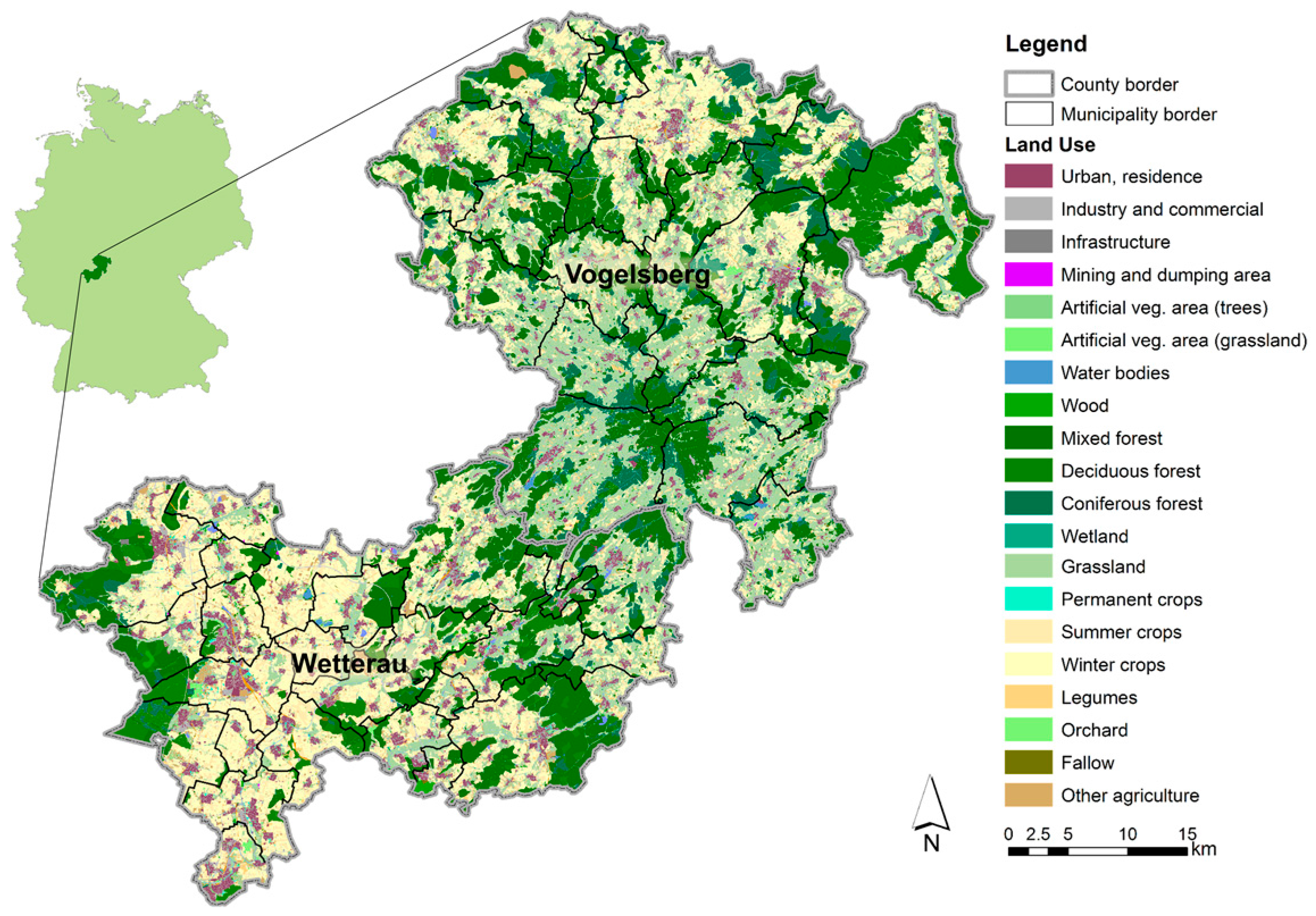
2.1. Study Region

The case study area encompasses the counties Wetterau and Vogelsberg located in Hesse, Germany (Figure 1) and covers an area of 2557 km2 subdivided into 44 municipalities with areas ranging from 12 to 141 km2. The counties represent a typical mosaic of cultural landscapes in central Europe with different climate, topography, soils, and land use.
The county Wetterau (Figure 1, annual precipitation 635 mm, annual average temperature 8.9 °C at Bad Nauheim 148 m a.s.l., period 1961–1990) lies in the rain shadow of the low mountain range Taunus and is distinctly drier than the Vogelsberg [40]. Due to the very fertile loess-rich soils of the Wetterau, the area is predominantly used for intensive agriculture, especially crop production, which comprises more than 40% of the total area, the share of forest and grassland is comparatively small (28% and 14% respectively). This region is one of the oldest cultural landscapes in Germany with evidence for agricultural land use since the Neolithic. Due to its location close to metropolitan area of Frankfurt the county is an economically prospering region with growing industries and a high population density of 268 inhabitants per km2 [41].
The Vogelsberg (Figure 1) region is a low mountain range of volcanic origin. The higher areas within the Vogelsberg have high precipitation rates (annual precipitation 1307 mm, annual mean temperature 5.6 °C at Hoherodskopf 743 m a.s.l., period 1961–1990) and a relatively long period of snow cover [40]. Due to its geographical characteristics, the agricultural areas in the Vogelsberg are dominated by high share of grassland used for livestock production. The Vogelsberg region has a high share of forest (around 40%), and it has the lowest population density of Hesse with 73 inhabitants per km2 [41]. Furthermore, the Vogelsberg area is affected by demographic change and high emigration rates to prospering regions such as Frankfurt, leading to local population decline and abandonment of agricultural land. One important source of income is tourism with almost 500,000 overnight stays in the year 2013 [41]. In addition to its role in tourism, this county is one of the largest sources for drinking water in Germany and the main provider of drinking water for Frankfurt and the Rhein-Main area.

2.2. Assessment of Ecosystem Service Supply

Ecosystem services were classified according to the conceptual framework developed by the initiative ‘Common International Classification of Ecosystem Services (CICES)’ [44]. The selection of ecosystem services for this study was based on a priority list of ecosystem services in Germany [45] and on the availability of spatial data. In this paper, only ecosystem service supply was considered irrespective of demand [35]. Table 1 provides a summary of the indicators assessed.
We used publicly available datasets that can commonly be obtained for this type of landscape to derive generally applicable models. The land cover vector dataset ALKIS served as a basis for the indicators that we used in this study [42]. For the agricultural land cover types a finer classification was possible, overlaying the data with the Integrated Administration and Control System IACS data (InVeKoS, 43). Land cover types were split into 20 classes (Figure 1, see Appendix) and converted to a raster dataset of 10 m spatial resolution. All data were imported into ArcGIS 10.2.2 (ESRI) for visualization and data processing. Statistical analysis were performed using the R statistical software [46] (see Section 2.3). Ecosystem services were assessed at a 10 m spatial resolution using data for 2011 or as close as possible to this date.
The InVEST (Integrated Valuation of Ecosystem Services and Trade-offs) modeling tool [47,48] was used to assess the ecosystem services water provision, carbon storage and erosion control, while analyses in ArcGIS 10.2.2 were applied to evaluate food production, timber supply and outdoor recreation. Accuracy of ecosystem service estimates was assessed by comparing our model results with observed measurements (water provision) or census data for this region (timber supply, carbon storage). The ecosystem services food production, erosion control and recreational potential were assessed using regional adapted methods. Full details on methods to derive indicator values are provided in the following paragraphs. A list of spatial datasets used for the assessment of ecosystem service supply is provided in the supplementary material.

2.2.1. Water Provision

We mapped surface water yield as an indicator for the ecosystem service freshwater supply using InVEST. Surface water yield is defined as precipitation minus storage and evapotranspiration losses and therefore describes the amount of water that is discharged as surface flow [47]. The water yield model determines the net hydrological balance as the difference between precipitation and evapotranspiration [47,49], dependent on the characteristics of the vegetation and without distinguishing between surface, subsurface and base flow. In the InVEST 3.0.0 model version we used, the annual water yield ( Y x j ) provided from a cell in the landscape ( x = 1 , 2 , , X ) is calculated as follows:
Y x j = ( 1 A E T x j P x ) P
where A E T x j is the actual annual evapotranspiration on pixel x for landuse and land cover (LULC) j . P x is the annual precipitation on pixel x . For detailed description of methodology see [47,50]. Annual average precipitation and reference evapotranspiration in the study region were obtained from the German Weather Service [51] for the period 1995–2004. From the soil map (vector dataset) of Hesse [52] root restricting layer depth and plant available water content were derived. The latter was obtained by dividing the fraction of volumetric field capacity by soil depth [47]. Both parameters were converted to a raster dataset of 10 m spatial resolution. For each LULC category specific evapotranspiration coefficients Kc and the root depth were determined based on coefficients reported in the literature (see Appendix). The empirical constant Z that captures the local precipitation pattern and hydrogeological characteristics was determined according to the following equation [53,54]:
Z = ( ω 1.25 ) P A W C
where P and A W C are average values of precipitation and available water capacity in the study area. The empirical catchment parameter ω was taken from literature [53]. Based on estimates of our regional catchments [55] we calculated a seasonality factor Z of 4.
Validation of the water yield application was performed by comparing InVEST water yield results with aggregated observed runoff values [56]. Observed surface flow for twelve sub-watersheds distributed across and within the study area for the period from 1995 to 2004 was provided by the Hessian Agency for Nature Conservation, Environment and Geology (HLUG). To validate the model, we compared the results through the calculation of the Nash-Sutcliff model efficiency index [57]. The obtained index result was 0.62 (R2 = 0.70), which indicates that InVEST represented the water flow in the study area sufficiently well.

2.2.2. Timber Supply

A key provisioning service of forests is the supply of timber and fuel wood [58]. Large parts of the study area are covered by forests, and timber production is the most important source of income for forest owners in Hesse [59]. Ownership of forests in Hesse is diverse. In the study area, around 63% of the forest area is managed by the Hessian State Forest Enterprise, while the remaining 37% are privately owned.
The timber stock estimation for the Hessian State Forest Enterprise managed forests were based on national standardized forest inventory data [60]. The inventory provides information on stand area and tree parameters such as species, age, height, timber volume (m3·ha−1) and growth rates (m3·ha−1·year−1) on a vector base. The Hessian State Forest Enterprise reclassified forest cover into forest stand types based on the dominating tree species: spruce (Picea), pine (Pinus), Douglas fir (Pseudotsuga), oak (Quercus), beech (Fagus), mix of cherry-maple-ash-elm (Prunus, Acer, Fraxinus, Alnus), mix of birch-willow-poplar-rowan (Betula, Salix, Populus, Sorbus). Information on forest stand-age, coarse wood stocks in cubic meter of wood and average total growth per year were obtained from the forest inventory data. For the privately owned forests that are not managed by the Hessian State Forest Enterprise we estimated the average coarse wood stocks of deciduous (239 m3·ha−1), coniferous (312 m3·ha−1) and mixed forest (275 m3·ha−1) based on the data of the forest inventory. We assigned this information to privately owned forest stands of the LULC data. All timber stock information (including both forest stands managed by the Hessian State Forest Enterprise and privately managed) was converted to a raster dataset of 10 m spatial resolution.
We compared our results to estimates obtained by the Third German National Forest Inventory [61] at federal state level. For this assessment, the average calculated timber stock was calculated over the whole study region. According to the National Forest Inventory [61] the average timber stock in forests in Hesse is 276 m3·ha−1; we calculated a similar average of 288.59 m3·ha−1 for timber stock in the counties Vogelsberg and Wetterau.

2.2.3. Food Production

To assess the potential of the landscape to produce food we used a frequently applied approach [31,62] of mapping the soil fertility of arable land. Food production depends heavily on natural ecosystem conditions as well as on the management by farmers. For this ecosystem service, the challenge is to separate the relative roles of natural soil conditions and technical measures such as liming, fertilization, plant protection and irrigation. Only the contribution of natural conditions is considered as part of the ecosystem service food production [31,63] and included here. The production of fodder on grassland for animal consumption is not considered in this indicator. To assess the natural potential of the soil to produce crops we mapped potential soil fertility of arable land based on a method recommended for this region of Friedrich and Vorderbrügge [64] using vector based digital soil maps [52] in which water holding capacity, soil moisture and carbonate content were classified into categories and subsequently aggregated to five soil fertility classes. These soil fertility information was subsequently converted to a raster dataset of 10 m spatial resolution. To assess the soil fertility classes of arable fields, we overlaid the soil fertility map with arable land pixels of the LULC dataset.

2.2.4. Carbon Storage

We estimated the amount of carbon stored in the study region by combining the InVEST carbon model with detailed information on wood biomass of forests. The InVEST-toolbox provides a theoretical but comparatively simple production function to assess the capacity of ecosystems to store carbon by summing three major carbon pools: aboveground biomass, belowground biomass and carbon stored in the soil [48]. The carbon pool dead organic matter was not included in this study. The main inputs into the model were a land use map together with a database of the amount of carbon stored for each LULC category for the three carbon pools above- and belowground biomass and soil to 30 cm depth (see Appendix). These input values were derived from the National Inventory Report for the German Greenhouse Gas Inventory 1990–2011 [65]. Since detailed information on wood biomass of forest stands are available (see Section 2.2.2 Timber Supply) we added this information to the carbon model to derive total carbon stocks across the landscape.
To estimate the carbon stocks in aboveground and belowground biomass of forested areas, the timber volume estimations of national standardized forest inventory [60] was used. For privately managed forests that are not covered by the aforementioned inventory, we calculated average coarse wood stocks, according to the following equation (Equation (3)), following Pistorius et al. [66]:
C = ( D   r d   B E F )   ( 1 + R )   C F
where C is the total carbon in biomass for each forest category; D is the growing stock volume (m3·ha−1); rd is the stem bulk density; BEF is the biomass expansion factor; R is the root to shoot ratio and CF is the carbon fraction of dry matter.
The factors used to convert raw-wood volume D to dry matter, the bulk density rd, was taken from Knigge and Schulz [67]. Since the available inventory do not contain information about tree biomass other than coarse wood stocks, we applied the literature based biomass expansion factors BEF to account for the biomass of small wood and needles, respectively [65,68]. The root to shoot ratio R for trees was estimated according to the German inventories under UNFCCC [65]. To calculate the carbon fraction CF of biomass, density was set to 0.5 which is used in accordance with the IPCC Guidelines [69]. The carbon stored in forest biomass was added to the above estimates on non-forest biomass and mineral soil carbon stock to provide estimates of the carbon stored across the landscape.

2.2.5. Erosion Control

The ability of the landscape to retain soil is mainly determined by the intensity of rainfall, soil properties, topography, vegetation, and anthropogenic factors such as agricultural practices [70]. Permanent vegetation types act as sinks for sediment including nutrients, pesticides and other agro-chemicals as they interrupt the movement from upslope agricultural areas to surface waters [31,36,71].
Using the Universal Soil Loss Equation (USLE) [70] implemented in the Sediment Delivery Ratio module of InVEST [47] and regional recommendations of input variables, the potential soil loss of each land use cell was calculated as:
A = R   K   L S   C   P
where A is the potential long-term annual soil loss (t ha−1), R is the erosivity factor of the rain, K is the soil erodibility factor, LS is the slope length and steepness factor, C is the land cover management factor, and P is the supporting practice factor [72]. The value of the retention service is computed by finding the difference between the sediment export from a hypothetical scenario where all land is cleared to bare soil (RKLS) and potential soil loss (A) of the current landscape. To meet regional standardizations we followed guidelines of the Hessian Agency for the Environment and Geology [73] to calculate the factors for the USLE. The rainfall erosivity map was generated for the study region following the method of Schwertmann et al. [74]:
R   =   0.141   P r e c i p   S u m m e r   1.48
where P r e c i p   S u m m e r is the long-term (1981 to 2011) average precipitation of the summer months May to October obtained from the German Weather Service [51]. Soil erodibility was estimated by combining characteristics of soil type, organic matter content, and soil texture using the method of DIN 19708 [75]. The slope length and steepness factors LS was calculated using a digital elevation model [55].The land cover specific C factor was assigned using values obtained from the literature (see Appendix) on a more detailed land use map which discriminates between crop types [43]. To detect areas, which contribute to retention, the Sediment Delivery Ratio model computed the so-called sediment retention index as avoided soil loss by the current land use compared to bare soil.

2.2.6. Outdoor Recreation

Outdoor recreation values are defined as the ability of landscapes to provide opportunities for nature-based recreational activities such as hiking, outdoor sports, camping, bird-watching and fishing [62]. The ecosystem function ‘recreational potential’ was mapped through a composite indicator based on Paracchini et al. [76]. According to findings from surveys and from literature, recreation potential depends on three different components of people´s behavior and preference for outdoor recreation: the first relates to peoples preference for more natural areas and concerns the degree of naturalness [77]; the second refers to protected areas as they are considered indicators of high natural value [78]; the third component refers to the attractiveness of water bodies [79].
The degree of naturalness is modeled based on the hemeroby index which measures the human influence on landscapes and vegetation and ranges from 1 (natural—without actual human impact) to 7 (artificial) [1]. The naturalness was obtained by attributing to each land cover class its degree of naturalness based on the European hemeroby map of Paracchini and Capitani [77]. Protected areas were mapped using information from the Natura 2000 database of the Birds and the Habitat Directive [80] and other designated areas defined in Germany’s Federal Nature Conservation Act [81] such as Landscape Protection Areas, Nature Conservation Areas and Nature Parks [82]. Other designated areas such as National Parks and Biosphere Reserves were not present in the case study area. The attractiveness of water bodies was estimated by calculating the distance to all surface water bodies. We included all stagnant water bodies extracted from the LULC dataset and water courses of the first and second order [42]. Small streams of the third order where not included.
We assumed that each component covers a different aspect of outdoor recreation. After normalizing each variable to a range to 0–1 using a Min-Max normalization method [83] the three components have been aggregated considering each variable equally important therefore given equal weights [76]. We identified areas with high recreational potential, hereinafter “recreational hotspots”, by extracting the patches within the upper 25th percentile [18]. This analysis addressed recreation and not tourism, ranging from a short walk or bicycle ride to a Sunday hiking trip. Long distance travelling (>100 km) was not included in the study as the current analysis focused on resident populations.

2.3. Spatial Relationships among Ecosystem Services

Individual ecosystem services were mapped to visualize and compare their spatial patterns. We calculated summary statistics and evaluated the degree for spatial clustering of each service using Moran’s I of package “raster” [84]. We identified service provisioning hotspots and coldspots of each service and the spatial congruence of those for multiple service supply. Grid cells in the study area that were within the upper 25th percentile were defined as individual hotspots, and those within the lowest 25th percentile were considered as individual coldspots. Hotspots and coldspots of multiple services were defined as those areas where at least four services were supplied in the upper 25th, respective the lower 25th percentile. Spatial patterns of hotspots and coldspots were analyzed by computing the proportion of the study area occupied, the patch density and the mean patch area in R using ClassStats of the package “SDMTools” [85,86].
Analyzing the interactions between pairs of ecosystem services took place on a municipal level. The municipal boundaries were taken from the Administrative Map of Germany [87]. The area of each municipality was calculated based on these boundaries. The administrative boundaries were used to identify trade-offs and synergies spatial variables on the supply of ecosystem services. Municipal level was chosen since these administrative units represent the smallest unit of governance and political decision making (such as landscape and land-use planning). Because the municipalities are not all of the same size (area ranges from 12 to 141 km2, mean 58 km2) we aggregated the sets of ecosystem service associated with each municipality (n = 44) by extracting the mean values of individual ecosystem services indicators per municipality. Non-normally distributed indicators were transformed (water provision x0.2, food production x0.3 erosion control x0.5, recreational potential x0.2) using the Box-Cox transformation of the “MASS” package [88] before statistical analyses. The transformed data were standardized by ranging the data to a scale from zero to one based on minimum and maximum values to allow for meaningful comparisons of all indicators [89]. Graphical and correlation analysis were performed to examine interactions between pairs of ecosystem services. For correlation analysis, the Pearson parametric correlation test was used to assess correlation coefficients for all pairs of ecosystem services. For graphical analysis we used a bivariate version of the boxplot, the bagplot [90]. We calculated bagplots for all possible pair-wise comparisons using the package “aplpack” [91]. Synergetic relationship between two ecosystem services was illustrated in the bagplot when the plot was oriented from the lower left to upper right and thus covering the negative/negative and positive/positive space. Trade-offs between two ecosystem services are expected if the bagplot is oriented from the upper left to the lower right.

3. Results

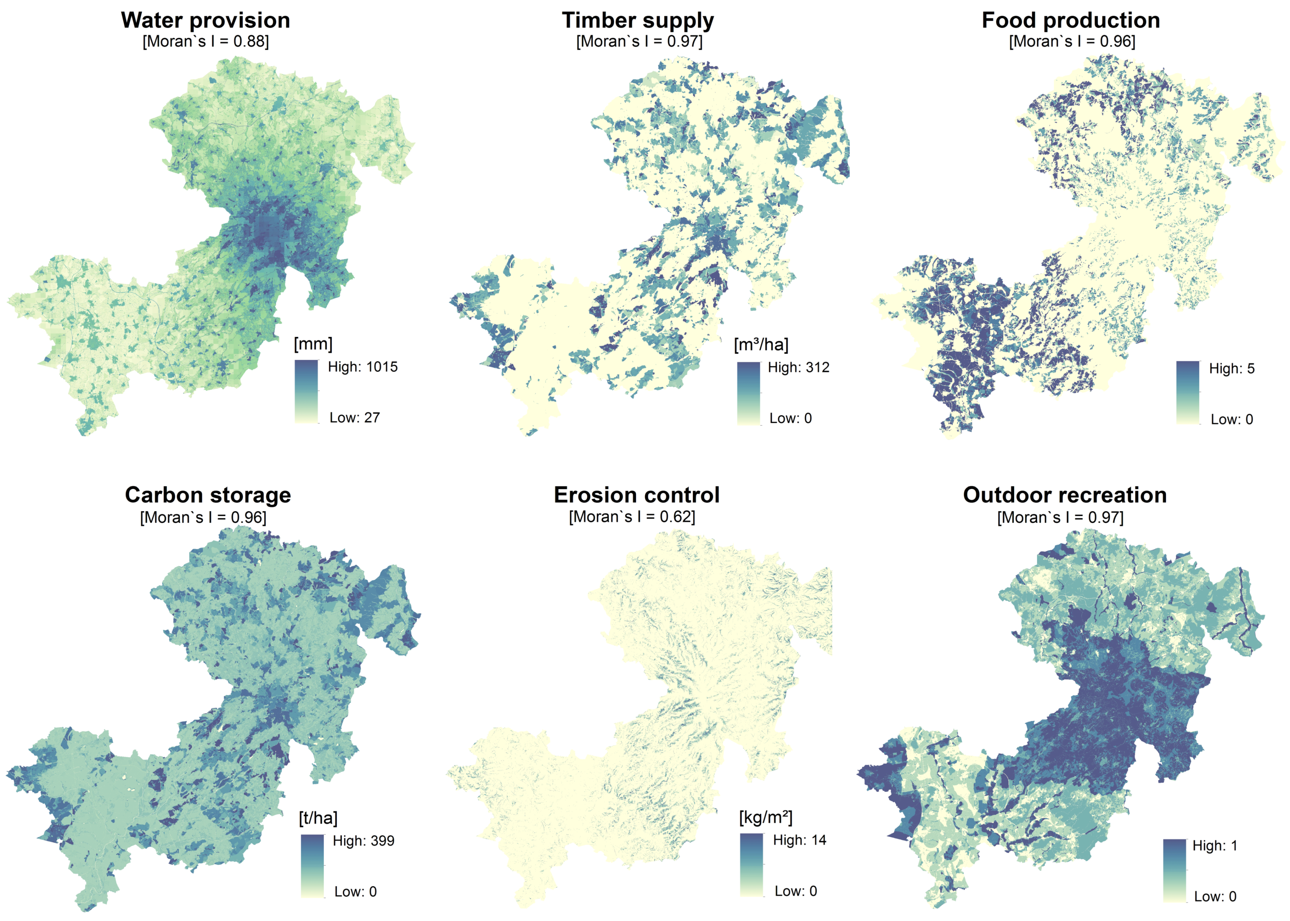
3.1. Spatial Patterns of Ecosystem Service Supply

Supply of individual ecosystem services (measured at a resolution of 10 m × 10 m) varied across the landscape (Figure 2) and showed a pronounced spatial clustering (all ecosystem services Moran’s I > 0.60). For descriptive statistics of each service, see Table 2. Within the study area on average 100 t·ha−1 of carbon are stored in the above- and belowground biomass and the soil. The biggest carbon pools can be found in the deciduous forest stands with carbon stocks above 250 t·ha−1. The sediment model showed an average potential soil loss of around 200,000 t·year−1 across the study area, with potential soil loss up to 14 kg·m−2. However, only 4300 t·year−1 are exported to streams and rivers, because most of the soil particles are retained by vegetation. Calculating the water provision of the study region revealed an average water yield of 255 mm·year−1. However, these values vary in space ranging from water yields under 100 mm in the Wetter valley up to over 800 mm in the mountainous region of the Vogelsberg with higher annual rainfall and lower evapotranspiration. The total standing stock of timber had a volume of more than 26 Mio. m3 across the study area with highest timber stocks in coniferous forest stands of 312 m3·ha−1. The total area of arable land cells in the two highest soil fertility classes comprises 138 km2 which represents around 12% of the counties. Regions of high recreational potential, so-called recreational hotspots, with values within the upper 25th percentile, cover only 1.20% (31 km2) of the study region. All ecosystem services are clustered according to ecological, geographic or social factors that led to land use systems and associated ecosystem services. For example, food production is found in rather flat, fertile regions of the study region, while timber is mainly provided from steeper slopes or higher elevations. There were similarities among the spatial distribution of the supply of different services (e.g., timber supply and carbon storage). However, the geographic distribution of the supply of individual ecosystem service revealed that each pattern was distinct. Timber for example is supplied in forest areas only, while carbon is stored in almost all land use types including agricultural areas. The quantities of supply vary, leading to distinct patterns of the respective ecosystem services.
Only 5% of the landscape was occupied by ecosystem service hotspots, where at least four services were provided in the upper 25th percentile (Figure 3a). These areas often coincided with forest areas and other wooded structures in mountainous areas and were few in number and rather large in size (patch density = 7.4 km−2, mean patch area = 60.9 ha). Coldspots, which are areas where at least four services were produced in the lower 25th percentile, occupied around 20% of the landscape (Figure 3b) and corresponded with cropland, urban areas and other sealed areas. Coldspots were more numerous and slightly smaller in size (patch density = 35.3 km−2, mean patch area = 57.3 ha).

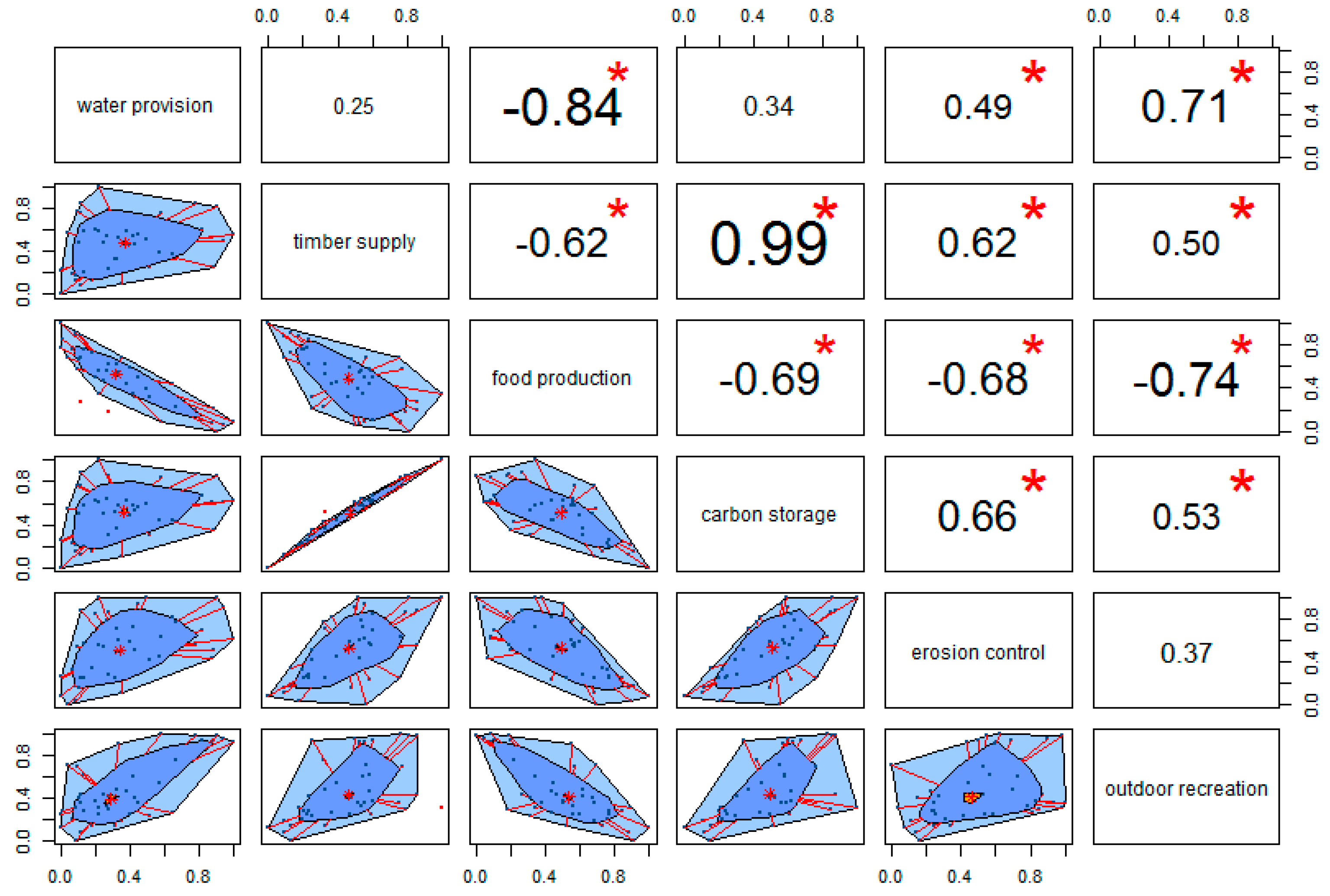
3.2. Relationships among Ecosystem Services

Analysis of relationships of ecosystem service supply was carried out at the municipal level. Most of the ecosystem services were correlated (Figure 4). Correlations were highly significant for twelve out of 15 pairs of ecosystem services (p-value < 0.001). The relationship between regulating services (carbon storage and erosion control) and the provision of timber was synergistic. The cultural ecosystem service outdoor recreation was found to have a positive relationship with areas of high water supply (r = 0.71). Food production was negatively correlated with all other ecosystem services included in this study, indicating a trade-off. The ecosystem service pairs water provision vs. timber supply (r = 0.25) water provision vs. carbon storage (r = 0.34) and erosion control vs. outdoor recreation (r = 0.37) were not significantly correlated.

4. Discussion

4.1. Assessment of Ecosystem Service Supply

We aimed to assess spatial variability in the supply of multiple ecosystem goods and services in the study region. To evaluate ecosystem services in a replicable and standardized manner [92,93,94], we used biophysical proxies based on datasets that are typically available in this type of landscape, and models which can be applied in other locations. The ecosystem service indicators reflect the capacity of ecosystems to provide services based on present knowledge of ecological relationships. However, for many of the ecosystem services we rely on simplified indicators to estimate the natural potential of providing these services [95]. The use of relatively simple ecosystem service models such as InVEST enables the extension to other study locations, the assessment of multiple services and may also generate greater transparency and trust among users [94].
In the models, neither spatial flow dynamics such as down-stream effects of landscape features on ecosystem service performance nor feedbacks between ecosystem services and temporal variability were taken into account. The erosion control model for example does not consider feedbacks of sedimentation processes on water quality and quantity or carbon storage. Moreover, the erosion control model uses long-term average summer precipitation data to derive the erosivity factor. However, extreme precipitation events (either within or outside of summer season) may result in dramatic soil losses. The used model is not able to detect temporal variability of sediment erosion. Further, specific landscape features such as wetlands or hedges can have disproportionate effects on various ecosystem services dependent on their position in the landscape. This information is essential for strategic spatial positioning of key landscape elements to improve multiple ecosystem services [96].
The carbon storage model does not consider the full carbon cycle or fluxes among carbon pools [47]. In addition, it relies on carbon storage estimates derived from land use classes and does not consider other controlling factors for carbon storage such as climate, soil depth or management practices [47,97]. The freshwater model is also based on simplifications of well-known hydrological relationships [27,56] and works on an annual basis. Seasonal variability in the delivery of hydrological ecosystem services is not considered here. Furthermore, we did not include water withdrawal in the freshwater model which could lead to a general inaccurate estimation of water provision [98]. Neglecting ecosystem service flow dynamics and feedbacks may lead to over- or underestimation of ecosystem service supply. Modeling approaches that incorporate service-specific sources, sinks, users, spatial flows and interactions can provide a more complete understanding of ecosystems services [94,99]. Although more complex modeling approaches may more accurately represent natural processes and interactions, the potential gains in accuracy associated with this must be weighed against the increased complexity and reduced generalizability [47].
In applying the models, a conversion of (polygon) vector datasets (land use, soil information, protected areas and forest inventory data, see supplementary material) to raster format was necessary. This transformation, however, may produce considerable distortion in landscape pattern characteristics (e.g., cut cells or loss of small or thin elements) and, hence, in the outcome of the ecosystem service assessment [100]. In order to maintain the integrity of our data and reduce the loss of geometric precision we used a fine spatial resolution of 10 m.
These limitations could lead to inaccurate estimates of ecosystem service supply. For most ecosystem services, however, we were able to assess the accuracy of our estimates by validation (potential water provision) or comparison with other statistical estimations (potential timber supply) or applied the model according to regional knowledge (e.g., potential carbon storage, potential erosion control) to minimize overall uncertainty.

4.2. Relationships among Multiple Ecosystem Services

To derive total ecosystem service supply we calculated multiple ecosystem service hotspots and coldspots, respectively, which represents the capacity to provide multiple services. This method does not include the demand for the particular ecosystem service. To improve the method of defining hotspots and coldspots we propose to investigate which ecosystem services are below a critical threshold in relation to demand [35]. Adding up of the supply of ecosystem services to evaluate multifunctionality, does take interaction among ecosystem services indirectly into account (e.g., carbon storage and timber supply) since they are both included independently of each other. Comparison of cumulative ecosystem service supply (represented by hotspots or coldspots) with land use information suggests a strong correlation with forest, woodland and grassland rich regions. The abundance and spatial organization of fields, hedgerows, grassland and forest patches determine to large parts the ecosystem service supply [9]. Our results, however, depend on the set of ecosystem services analyzed. Nonetheless, these results support existing knowledge about links between landscape structure and ecosystem services [17,37,38], proposing that methods applied here can be applied to other cultural landscapes.
Correlations between ecosystem services analyzed in this study were found to be stronger than those between different ecosystem services found in a paper from Jopke et al. [38,101]. This may be due to the much larger European Union wide spatial scale at which this study was conducted (NUTS 3 level across Europe), the number of services assessed and different proxies used. The scale of the analysis will to some extent control the intensity of interactions. We suggest the spatial scale of municipalities to be small enough so that variables that determine the supply of one service will also have similar effects on the supply of other services. The comparison of our outcomes with a study conducted in Quebec, Canada on a municipal level with comparable size of administrative units (averaging 74 km2) revealed similar results [37].
Among all studied ecosystem services pairs, most showed a synergetic relationship, and correlations were significant. Some ecosystem service pairs showed no significant correlation. Erosion control and outdoor recreation showed no significant correlation which may be because the recreational potential of the landscape is determined by the degree of naturalness, designated areas and water areas which are seldom located in arable areas of high erosion control. Water provision was not correlated to timber supply and carbon storage. This may be due to the fact that precipitation patterns, which control water yield, follow a topographic gradient while forest areas with high rates of timber supply and carbon storage are distributed across the study area. All ecosystem services showed trade-offs against crop production. Analyses of interactions among ecosystem services in Quebec, Canada and Europe respectively lead similarly to the conclusion that crop production is the most conflicting ecosystem service [37,38,78]. Our analysis, though, shows only correlational relationships, yet causal relationships cannot be proved [27]. However, there seems to be a general trade-off between crop production and regulating or cultural services. Regions rich in arable production essentially produce crops and are relatively poor in delivering other ecosystem services. Among all other considered services, synergies were found. Regions rich in green infrastructure such as hedges, wetlands and forests provide a wide array of services. Landscape composition and landscape diversity are important determinants of ecosystem services.
The results presented in this manuscript have practical uses for landscape management, spatial planning and policy in the analyzed counties. Spatial explicit assessment of ecosystem service supply will help to identify priority regions for landscape management to promote landscape multifunctionality. Having identified trade-off regions can help decision-making in targeting management actions (e.g., implementation of agri-environmental schemes). To secure the overall supply of ecosystem services the development of green infrastructure should be especially promoted in the intensive agricultural areas of the counties Wetterau and Vogelsberg. Furthermore, the impact on ecosystem provision from a proposed landscape alteration will be more thoroughly evaluated if improvements or declines in analyzed ecosystem services can be demonstrated to stakeholders. Finally, assessment of ecosystem services will be used in reaching decision that consider the full effects of a proposed use of an ecosystem, rather than just those costs or values that enter markets in the form of private goods [96]. Ecosystem service assessment methods like the ones applied should be included in spatial planning in order to identify priority regions for management actions and consider consequences of land use changes for different ecosystem services. Ecosystem service assessment can improve landscape planning and decision-making and control for a sustainable use of ecosystem services.

5. Conclusions

We provide a methodological framework for mapping and analyzing multiple ecosystem services in a spatially explicit way. Using this framework, we exposed positive, negative and neutral relationships among ecosystem services at the municipal level. Our study demonstrates that ecosystem service supply shows distinct spatial clustering. We found positive relations among water provision, timber supply, carbon storage, erosion control, and outdoor recreation, but trade-offs between food production and all other services. Highlighting these patterns is a prerequisite for optimizing multiple ecosystem services through adaptive land-management decisions. Applying this knowledge in practice requires that social and ecological drivers of change in supply of and demand for ecosystem service are further investigated. A mechanistic understanding of the feedbacks between drivers, ecosystem services and societal responses to ecosystem service change is needed to achieve targeted management schemes that ensure long-term, balanced provision of ecosystem services.

Supplementary Materials

The following are available online at www.mdpi.com/2073-445X/5/2/17/s1.

Acknowledgments

This study was supported by the Federal Ministry for Education and Research (BMBF) in the project JAGUAR (Project-ID 01LC1106A). We are grateful to all colleagues working on this project for continuous discussion and support. Finally, we thank three anonymous reviewers, who helped us to improve the quality of this paper.

Author Contributions

A.F.-M. performed the ecosystem service assessment, analyzed the data, and wrote the paper; A.F.-M., L.B. and T.K. designed the study; S.H., L.B., V.W. and T.K. contributed to writing the manuscript; S.H. and V.W. initiated and coordinated the research project; all authors read and approved the final manuscript.

Conflicts of Interest

The authors declare no conflict of interest.

Appendix

Biophysical table with input parameter to model carbon storage, sediment retention and water yield including References: Carbon stock estimates for above- and belowground biomass and soil to 30 cm depth; land cover management factor C, supporting practice factor P, maximal rooting depth and evapotranspiration coefficients Kc.
Table A1. Biophysical table with input parameter to model carbon storage, sediment retention and water yield: Carbon stock estimates for above- and belowground biomass and soil to 30 cm depth; land cover management factor C, supporting practice factor P, maximal rooting depth and evapotranspiration coefficients Kc.
LULC DescriptionDetailed Crop DescriptionCarbon StorageErosion ControlWater Provision
Aboveground BiomassBelowground BiomassSoil (30 cm)USLE CUSLE PMax. Rooting DepthKc
(Mg·ha−1)(Mg·ha−1)(Mg·ha−1) (mm)
[65,65][65][65][73,102] [103,104,105,106][107]
Urban, residence 9.913.558.670.01100
Industry and commercial 9.913.558.670.01100
Infrastructure 0058.670.001100
Mining and dumping area 0055.60.2100
Artificial veg. area (tree dom.) 9.913.558.670.001129300.85
Artificial veg. area (grass dom.) 9.913.558.670.004114400.69
Water bodies 0000.00115001.25
Wood 35.2711.6673.180.001122701.02
Mixed forest According to forest inventoryAccording to forest inventory62.450.001134801.01
Deciduous forest According to forest inventoryAccording to forest inventory62.450.001134801.02
Coniferous forest According to forest inventoryAccording to forest inventory62.450.001134601
Abandoned area 4.362.3355.60.004133000.69
Wetland 14.675.44740.004127000.81
Grassland 4.362.3377.430.004127000.69
Permanent crops 8.232.9955.60.03111000.55
Summer cropscorn-cob-mix6.051.4360.030.35112000.81
durum wheat6.051.4360.030.12112000.81
maize6.051.4360.030.35112000.81
oats6.051.4360.030.14112000.81
potatoes6.051.4360.030.29112000.81
spring barley6.051.4360.030.17112000.81
spring wheat6.051.4360.030.14112000.81
sugar beet6.051.4360.030.32112000.81
summer rapeseed6.051.4360.030.1112000.81
sweet corn6.051.4360.030.35112000.81
other summer crops6.051.4360.030.12112000.81
Winter cropsrye6.051.4360.030.08110100.87
spelt6.051.4360.030.12110100.87
triticale6.051.4360.030.12110100.87
winter barley6.051.4360.030.07110100.87
winter oats6.051.4360.030.2110100.87
winter rapeseed6.051.4360.030.1110100.87
winter wheat6.051.4360.030.12110100.87
other winter crops6.051.4360.030.1110100.87
Legumesalfalfa6.051.4360.030.03118500.78
beans6.051.4360.030.3118500.78
clover6.051.4360.030.03118500.78
clover-alfalfa-mix6.051.4360.030.03118500.78
lupine6.051.4360.030.3118500.78
other legumes6.051.4360.030.07118500.78
peas6.051.4360.030.2118500.78
Orchard 8.232.9973.180.03124000.99
Fallow 4.362.3377.430.004127000.69
Other agriculture 6.051.4360.030.2110100.87

References

  1. Wrbka, T.; Erb, K.H.; Schulz, N.B.; Peterseil, J.; Hahn, C.; Haberl, H. Linking pattern and process in cultural landscapes. An empirical study based on spatially explicit indicators. Land Use Policy 2004, 21, 289–306. [Google Scholar] [CrossRef]
  2. Jongeneel, R.A.; Polman, N.B.P.; Slangen, L.H.G. Why are Dutch farmers going multifunctional? Land Use Policy 2008, 25, 81–94. [Google Scholar] [CrossRef]
  3. Koschke, L.; Fürst, C.; Frank, S.; Makeschin, F. A multi-criteria approach for an integrated land-cover-based assessment of ecosystem services provision to support landscape planning. Ecol. Indic. 2012, 21, 54–66. [Google Scholar] [CrossRef]
  4. Hauck, J.; Schweppe-Kraft, B.; Albert, C.; Goerg, C.; Jax, K.; Jensen, R.; Fuerst, C.; Maes, J.; Ring, I.; Hoenigova, I.; et al. The Promise of the Ecosystem Services Concept for Planning and Decision-Making. GAIA Ecol. Perspect. Sci. Soc. 2013, 22, 232–236. [Google Scholar]
  5. Zhang, W.; Ricketts, T.H.; Kremen, C.; Carney, K.; Swinton, S.M. Ecosystem services and dis-services to agriculture. Ecol. Econ. 2007, 64, 253–260. [Google Scholar] [CrossRef]
  6. Billeter, R.; Liira, J.; Bailey, D.; Bugter, R.; Arens, P.; Augenstein, I.; Aviron, S.; Baudry, J.; Bukacek, R.; Burel, F.; et al. Indicators for biodiversity in agricultural landscapes: A pan-European study. J. Appl. Ecol. 2008, 45, 141–150. [Google Scholar] [CrossRef]
  7. Power, A.G. Ecosystem services and agriculture: tradeoffs and synergies. Philos. Trans. R. Soc. B Biol. Sci. 2010, 365, 2959–2971. [Google Scholar] [CrossRef] [PubMed]
  8. Rodriguez, J.P.; Beard, T.D.; Bennett, E.M.; Cumming, G.S.; Cork, S.J.; Agard, J.; Dobson, A.P.; Peterson, G.D. Trade-offs across space, time, and ecosystem services. Ecol. Soc. 2006, 11. [Google Scholar]
  9. van Zanten, B.T.; Verburg, P.H.; Espinosa, M.; Gomez-y-Paloma, S.; Galimberti, G.; Kantelhardt, J.; Kapfer, M.; Lefebvre, M.; Manrique, R.; Piorr, A.; et al. European agricultural landscapes, common agricultural policy and ecosystem services: A review. Agronom. Sustain. Dev. 2014, 34, 309–325. [Google Scholar] [CrossRef]
  10. Hodge, I.; Hauck, J.; Bonn, A. The alignment of agricultural and nature conservation policies in the European Union. Conserv. Biol. 2015, 29, 996–1005. [Google Scholar] [CrossRef] [PubMed] [Green Version]
  11. Strohbach, M.W.; Kohler, M.L.; Dauber, J.; Klimek, S. High Nature Value farming: From indication to conservation. Ecol. Indic. 2015, 57, 557–563. [Google Scholar] [CrossRef]
  12. de Groot, R.S. Function-analysis and valuation as a tool to assess land use conflicts in planning for sustainable, multi-functional landscapes. Landsc. Urban Plan. 2006, 75, 175–186. [Google Scholar] [CrossRef]
  13. Galler, C.; von Haaren, C.; Albert, C. Optimizing environmental measures for landscape multifunctionality: effectiveness, efficiency and recommendations for agri-environmental programs. J. Environ. Manag. 2015, 151, 243–257. [Google Scholar] [CrossRef] [PubMed]
  14. Millennium Ecosystem Assessment. Ecosystems and Human Well-being: Current State and Trends; Island Press: Washington, DC, USA, 2005. [Google Scholar]
  15. Carpenter, S.R.; Mooney, H.A.; Agard, J.; Capistrano, D.; DeFries, R.S.; Diaz, S.; Dietz, T.; Duraiappah, A.K.; Oteng-Yeboah, A.; Pereira, H.M.; et al. Science for managing ecosystem services: Beyond the Millennium Ecosystem Assessment. Proc. Natl. Acad. Sci. USA 2009, 106, 1305–1312. [Google Scholar] [CrossRef] [PubMed]
  16. Seppelt, R.; Dormann, C.F.; Eppink, F.V.; Lautenbach, S.; Schmidt, S. A quantitative review of ecosystem service studies: Approaches, shortcomings and the road ahead. J. Appl. Ecol. 2011, 48, 630–636. [Google Scholar] [CrossRef]
  17. Bennett, E.M.; Peterson, G.D.; Gordon, L.J. Understanding relationships among multiple ecosystem services. Ecol. Lett. 2009, 12, 1394–1404. [Google Scholar] [CrossRef] [PubMed]
  18. Qiu, J.; Turner, M.G. Spatial interactions among ecosystem services in an urbanizing agricultural watershed. Proc. Natl. Acad. Sci. USA 2013, 110, 12149–12154. [Google Scholar] [CrossRef] [PubMed]
  19. Paudyal, K.; Baral, H.; Burkhard, B.; Bhandari, S.P.; Keenan, R.J. Participatory assessment and mapping of ecosystem services in a data-poor region: Case study of community-managed forests in central Nepal. Ecosyst. Serv. 2015, 13, 81–92. [Google Scholar] [CrossRef]
  20. Zarandian, A.; Baral, H.; Yavari, A.; Jafari, H.; Stork, N.; Ling, M.; Amirnejad, H. Anthropogenic Decline of Ecosystem Services Threatens the Integrity of the Unique Hyrcanian (Caspian) Forests in Northern Iran. Forests 2016, 7. [Google Scholar] [CrossRef]
  21. Sherrouse, B.C.; Semmens, D.J.; Clement, J.M. An application of Social Values for Ecosystem Services (SolVES) to three national forests in Colorado and Wyoming. Ecol. Indic. 2014, 36, 68–79. [Google Scholar] [CrossRef]
  22. van Oort, B.; Bhatta, L.D.; Baral, H.; Rai, R.K.; Dhakal, M.; Rucevska, I.; Adhikari, R. Assessing community values to support mapping of ecosystem services in the Koshi river basin, Nepal. Ecosyst. Serv. 2015, 13, 70–80. [Google Scholar] [CrossRef]
  23. Burkhard, B.; Petrosillo, I.; Costanza, R. Ecosystem services—Bridging ecology, economy and social sciences. Ecol. Complex. 2010, 7, 257–259. [Google Scholar] [CrossRef]
  24. Baral, H.; Keenan, R.J.; Sharma, S.K.; Stork, N.E.; Kasel, S. Spatial assessment and mapping of biodiversity and conservation priorities in a heavily modified and fragmented production landscape in north-central Victoria, Australia. Ecol. Indic. 2014, 36, 552–562. [Google Scholar] [CrossRef]
  25. Nemec, K.T.; Raudsepp-Hearne, C. The use of geographic information systems to map and assess ecosystem services. Biodivers. Conserv. 2013, 22, 1–15. [Google Scholar] [CrossRef]
  26. Crossman, N.D.; Burkhard, B.; Nedkov, S. Quantifying and mapping ecosystem services. Int. J. Biodivers. Sci. Ecosyst. Serv. Manag. 2012, 8, 1–4. [Google Scholar] [CrossRef]
  27. Vigerstol, K.L.; Aukema, J.E. A comparison of tools for modeling freshwater ecosystem services. J. Environ. Manag. 2011, 92, 2403–2409. [Google Scholar] [CrossRef] [PubMed]
  28. Tallis, H.; Kareiva, P.; Marvier, M.; Chang, A. An ecosystem services framework to support both practical conservation and economic development. Proc. Natl. Acad. Sci. USA 2008, 105, 9457–9464. [Google Scholar] [CrossRef] [PubMed]
  29. Burkhard, B.; Kroll, F.; Müller, F.; Windhorst, W. Landscapes’ Capacities to Provide Ecosystem Services - a Concept for Land-Cover Based Assessment. Landscape Online 2009, 15, 1–22. [Google Scholar] [CrossRef]
  30. Termorshuizen, J.W.; Opdam, P. Landscape services as a bridge between landscape ecology and sustainable development. Landscape Ecology. 2009, 24, 1037–1052. [Google Scholar] [CrossRef]
  31. Lautenbach, S.; Kugel, C.; Lausch, A.; Seppelt, R. Analysis of historic changes in regional ecosystem service provisioning using land use data. Ecol. Indic. 2011, 11, 676–687. [Google Scholar] [CrossRef]
  32. Bastian, O.; Syrbe, R.-U.; Rosenberg, M.; Rahe, D.; Grunewald, K. The five pillar EPPS framework for quantifying, mapping and managing ecosystem services. Ecosyst. Serv. 2013, 4, 15–24. [Google Scholar] [CrossRef]
  33. Costanza, R.; d Arge, R.; de Groot, R.S.; Farber, S.; Grasso, M.; Hannon, B.; Limburg, K.; Naeem, S.; ONeill, R.V.; Paruelo, J.; et al. The value of the world’s ecosystem services and natural capital. Nature 1997, 387, 253–260. [Google Scholar] [CrossRef]
  34. Nelson, E.; Mendoza, G.; Regetz, J.; Polasky, S.; Tallis, H.; Cameron, D.R.; Chan, K.M.A.; Daily, G.C.; Goldstein, J.; Kareiva, P.M.; et al. Modeling multiple ecosystem services, biodiversity conservation, commodity production, and tradeoffs at landscape scales. Front. Ecol. Environ. 2009, 7, 4–11. [Google Scholar] [CrossRef]
  35. Burkhard, B.; Kroll, F.; Nedkov, S.; Müller, F. Mapping ecosystem service supply, demand and budgets. Ecol. Indic. 2012, 21, 17–29. [Google Scholar] [CrossRef]
  36. Brauman, K.A.; Daily, G.C.; Duarte, T.K.; Mooney, H.A. The nature and value of ecosystem services: An overview highlighting hydrologic services. Agric. Ecosyst. Environ. 2007, 32, 67–98. [Google Scholar] [CrossRef]
  37. Raudsepp-Hearne, C.; Peterson, G.D.; Bennett, E.M. Ecosystem service bundles for analyzing tradeoffs in diverse landscapes. Proc. Natl. Acad. Sci. USA 2010, 107, 5242–5247. [Google Scholar] [CrossRef] [PubMed]
  38. Jopke, C.; Kreyling, J.; Maes, J.; Koellner, T. Interactions among ecosystem services across Europe: Bagplots and cumulative correlation coefficients reveal synergies, trade-offs, and regional patterns. Ecol. Indic. 2015, 49, 46–52. [Google Scholar] [CrossRef]
  39. Ungaro, F.; Zasada, I.; Piorr, A. Mapping landscape services, spatial synergies and trade-offs. A case study using variogram models and geostatistical simulations in an agrarian landscape in North-East Germany. Ecol. Indic. 2014, 46, 367–378. [Google Scholar] [CrossRef]
  40. Deutscher Wetterdienst. Langjährige Mittelwerte 1961–1990, Aktueller Standort; 2015. Available online: https://www.dwd.de/DE/leistungen/klimadatendeutschland/langj_mittelwerte.html?lsbId=343278 (accessed on 14 December 2015).
  41. HGS. Hessische Gemeindestatistik 2014: Ausgewählte Strukturdaten aus Bevölkerung und Wirtschaft 2013, 35th ed.; Wiesbaden: Wiesbaden, Germany, 2015. [Google Scholar]
  42. HLBG. ALKIS®: Amtliches Liegenschaftskatasterinformationssystem; Hessische Verwaltung für Bodenmanagement und Geoinformation: Wiesbaden, Germany, 2006. [Google Scholar]
  43. HMUELV. InVeKoS: Integriertes Verwaltungs- und Kontrollsystem der Agrarverwaltung; Hessisches Ministerium für Umwelt, ländlichen Raum und Verbraucherschutz: Wiesbaden, Germany, 2011. [Google Scholar]
  44. Haines-Young, R.; Potschin, M. Common International Classification of Ecosystem Services (CICES): Consultation on Version 4. EEA Framework Contract No EEA/IEA/09/003 2012. Available online: http://cices.eu/wp-content/uploads/2012/07/CICES-V43_Revised-Final_Report_29012013.pdf (accessed on 3 March 2015).
  45. Marzelli, S.; Grêt-Regamey, A.; Moning, C.; Rabe, S.-E.; Koellner, T.; Daube, S. Die Erfassung von Ökosystemleistungen: Erste Schritte für eine Nutzung des Konzepts auf nationaler Ebene für Deutschland. Nat. Landsc. 2014, 89. [Google Scholar]
  46. R Development Core Team. R: A Language and Environment for Statistical Computing, Version 3.2.1; R Foundation for Statistical Computing: Vienna, Austria, 2015. [Google Scholar]
  47. Sharp, R.; Tallis, H.T.; Ricketts, T.; Guerry, A.D.; Wood, S.A.; Chaplin-Kramer, R.; Nelson, E.; Ennaanay, D.; Wolny, S.; Olwero, N.; et al. InVEST: InVest User’s Guide: Integrated Valuation of Environmental Services and Tradeoffs; The Natural Capital Project: Stanford, CA, USA, 2014. [Google Scholar]
  48. Kareiva, P.; Tallis, H.; Ricketts, T.H.; Daily, G.C.; Polasky, S. Natural capital: Theory and Practice of Mapping Ecosystem Services; Oxford University Press: New York, NY, USA, 2011. [Google Scholar]
  49. Terrado, M.; Acuna, V.; Ennaanay, D.; Tallis, H.; Sabater, S. Impact of climate extremes on hydrological ecosystem services in a heavily humanized Mediterranean basin. Ecol. Indic. 2014, 37, 199–209. [Google Scholar] [CrossRef]
  50. Sánchez-Canales, M.; López Benito, A.; Passuello, A.; Terrado, M.; Ziv, G.; Acuña, V.; Schuhmacher, M.; Elorza, F.J. Sensitivity analysis of ecosystem service valuation in a Mediterranean watershed. Sci. Total Environ. 2012, 440, 140–153. [Google Scholar] [CrossRef] [PubMed]
  51. DWD. CDC, Climate Data Center—Deutscher Wetterdienst. Available online: ftp://ftp-cdc.dwd.de/pub/CDC/ (accessed on 11 May 2014).
  52. HLUG. BFD50 Digitale Bodenflächendaten mit Sachdaten von Hessen 1:50000, 2012th ed.; Hessisches Landesamt für Umwelt und Geologie, FISBO (Fachinfomationssystem Boden/Bodenschutz): Wiesbaden, Germany, 2006. [Google Scholar]
  53. Xu, X.; Liu, W.; Scanlon, B.R.; Zhang, L.; Pan, M. Local and global factors controlling water-energy balances within the Budyko framework. Geophys. Res. Lett. 2013, 40, 6123–6129. [Google Scholar] [CrossRef]
  54. Donohue, R.J.; Roderick, M.L.; McVicar, T.R. Roots, storms and soil pores: Incorporating key ecohydrological processes into Budyko’s hydrological model. J. Hydrol. 2012, 436–437, 35–50. [Google Scholar] [CrossRef]
  55. HVBG. Digitales Geländemodell (DGM 10); Hessisches Landesamt für Bodenmanagement und Geoinformation: Wiesbaden, Germany, 2013. [Google Scholar]
  56. Hamel, P.; Guswa, A.J. Uncertainty analysis of a spatially explicit annual water-balance model: Case study of the Cape Fear basin, North Carolina. Hydrol. Earth Syst. Sci. Discuss. 2015, 19, 839–853. [Google Scholar] [CrossRef]
  57. Nash, J.E.; Sutcliffe, J.V. River flow forecasting through conceptual models part I—A discussion of principles. J. Hydrol. 1970, 10, 282–290. [Google Scholar] [CrossRef]
  58. Harrison, P.A.; Vandewalle, M.; Sykes, M.T.; Berry, P.M.; Bugter, R.; de Bello, F.; Feld, C.K.; Grandin, U.; Harrington, R.; Haslett, J.R.; et al. Identifying and prioritising services in European terrestrial and freshwater ecosystems. Biodivers. Conserv. 2010, 19, 2791–2821. [Google Scholar] [CrossRef]
  59. HMUKLV. Forests and Forestry in Hesse: Multipurpose Sustainable Forest Management Commitment for Generations; HMUKLV: Wiesbaden, Germany, 2012. [Google Scholar]
  60. FENA. Forsteinrichtung mit Sachdaten, 2014th ed.; State Forest Enterprise Hessen-Forst: Gießen, Germany, 2014. [Google Scholar]
  61. Thünen-Institut. Third German National Forest Inventory (2011–2012), Result Database. Available online: https://bwi.info (accessed on 6 November 2015).
  62. Maes, J.; Paracchini, M.-L.; Zulian, G. A European Assessment of the Provision of Ecosystem Services—Towards an Atlas of Ecosystem Services; Publications Office of the European Union: Luxembourg, 2011. [Google Scholar]
  63. Bastian, O.; Haase, D.; Grunewald, K. Ecosystem properties, potentials and services—The EPPS conceptual framework and an urban application example. Ecol. Indic. 2012, 21, 7–16. [Google Scholar] [CrossRef]
  64. Friedrich, K.; Vorderbrügge, T. Ertragspotenzial des Bodens. Available online: http://www.hlug.de/static/medien/boden/fisbo/bk/bfd50/extdoc/m_ertrag.html (accessed on 3 December 2015).
  65. NIR. National Inventory Report for the German Greenhouse Gas Inventory 1990–2011: Submission under the United Nations Framework Convention on Climate Change and the Kyoto Protocol; Umweltbundesamt: Dessau-Roßlau, Germany, 2013. [Google Scholar]
  66. Pistorius, T.; Zell, J.; Hartebrodt, C. Untersuchungen zur Rolle des Waldes und der Forstwirtschaft im Kohlenstoffhaushalt des Landes Baden-Württemberg; Forstliche Versuchs- und Forschungsanstalt Baden-Württemberg: Karlsruhe, Germany, 2006. [Google Scholar]
  67. Knigge, W.; Schulz, H. (Eds.) Grundriss der Forstbenutzung; Paul Parey Verlag: Hamburg and Berlin, Germany, 1966.
  68. Löwe, H.; Seufert, G.; Raes, F. Comparison of methods used within Member States for estimating CO2 emissions and sinks according to UNFCCC and EU Monitoring Mechanism: forest and other wooded land. Biotechnol. Agronom. Soc. Environ. 2000, 4, 315–319. [Google Scholar]
  69. Penman, J. Good Practice Guidance for Land Use, Land-Use Change and Forestry; Published by the Institute for Global Environmental Strategies for the IPCC: Kanagawa, Japan, 2003. [Google Scholar]
  70. Predicting Rainfall Erosion Losses—A Guide to Conservation Planning; Wischmeier, W.H.; Smith, D.D. (Eds.) US Government Printing Office: Washington, DC, USA, 1978.
  71. Dorioz, J.M.; Wang, D.; Poulenard, J.; Trevisan, D. The effect of grass buffer strips on phosphorus dynamics—A critical review and synthesis as a basis for application in agricultural landscapes in France. Agric. Ecosyst. Environ. 2006, 117, 4–21. [Google Scholar] [CrossRef]
  72. Renard, K.G. Predicting soil Erosion by Water: A Guide to Conservation Planning with the Revised Universal Soil Loss Equation (RUSLE); U.S. Department of Agriculture, Agricultural Research Service: Washington, DC, USA, 1997.
  73. HLUG. Bodenerosionsatlas Hessen. Hessisches Landesamt für Umwelt und Geologie 2014. Available online: http://www.hlug.de/start/boden/auswertung/bodenerosion/bodenerosionsatlas.html (accessed on 3 March 2015).
  74. Schwertmann, U.; Vogl, W.; Kainz, M. Bodenerosion durch Wasser: Vorhersage des Abtrags und Bewertung von Gegenmaßnahmen; Ulmer: Stuttgart, Germany, 1987. [Google Scholar]
  75. DIN 19708: Bodenbeschaffenheit—Ermittlung der Erosionsgefährdung durch Wasser mit Hilfe der ABAG; Deutsches Institut für Normung e.V.: Berlin, Germany, 2005.
  76. Paracchini, M.L.; Zulian, G.; Kopperoinen, L.; Maes, J.; Schaegner, J.P.; Termansen, M.; Zandersen, M.; Perez-Soba, M.; Scholefield, P.A.; Bidoglio, G. Mapping cultural ecosystem services: A framework to assess the potential for outdoor recreation across the EU. Ecol. Indic. 2014, 45, 371–385. [Google Scholar] [CrossRef] [Green Version]
  77. Paracchini, M.L.; Capitani, C. Implementation of a EU Wide Indicator for the Rural-Agrarian Landscape: In Support of COM(2006) 508 "Development of Agri-Environmental Indicators for Monitoring the Integration of Environmental Concerns into the Common Agricultural Policy"; Publications Office: Luxembourg, 2011. [Google Scholar]
  78. Maes, J.; Paracchini, M.L.; Zulian, G.; Dunbar, M.B.; Alkemade, R. Synergies and trade-offs between ecosystem service supply, biodiversity, and habitat conservation status in Europe. Biol. Conserv. 2012, 155, 1–12. [Google Scholar] [CrossRef]
  79. Kienast, F.; Degenhardt, B.; Weilenmann, B.; Waeger, Y.; Buchecker, M. GIS-assisted mapping of landscape suitability for nearby recreation. Landsc. Urban Plan. 2012, 105, 385–399. [Google Scholar] [CrossRef]
  80. EEA. European Inventory of Nationally Designated Areas 2005. Available online: http://www.eea.europa.eu/data-and-maps/data/nationally-designated-areas-national-cdda-9 (accessed on 23 February 2015).
  81. BNatSchG. Gesetz über Naturschutz und Landschaftspflege (Bundesnaturschutzgesetz) vom 25. März 2002: BGBl. I Nr. 51(German Nature Conservation Act); Bundesministerium der Justiz und für Verbraucherschutz: Berlin, Germany, 2009. [Google Scholar]
  82. HLUG. WMS Naturschutz 2015. Available online: http://www.hlug.de/start/geografische-informationssysteme/geodienste/naturschutz.html (accessed on 24 February 2015).
  83. Nardo, M.; Saisana, M.; Saltelli, A.; Tarantola, S.; Hoffman, A.; Giovannini, E. Handbook on Constructing Composite Indicators: Methodology and User Guide; OECD Publishing: Paris, France, 2005. [Google Scholar]
  84. Hijmans, R. Raster: Geographic Data Analysis and Modeling. Available online: http://CRAN.R-project.org/package=raster (accessed on 12 November 2015).
  85. McGarigal, K.; Cushman, S.A.; Neel, M.C.; Ene, E. FRAGSTATS: Spatial Pattern Analysis Program for Categorical Maps. Available online: http://www.umass.edu/landeco/research/fragstats/fragstats.html (accessed on 5 January 2016).
  86. VanDerWal, J.; Falconi, L.; Januchowski, S.; Shoo, L.; Storlie, C. Species Distribution Modelling Tools: Package ‘SDMTools’. Available online: http://www.rforge.net/SDMTools/ (accessed on 20 November 2015).
  87. Bundesamt für Kartographie und Geodäsie. Verwaltungsgebiete 1:250.000: © GeoBasis-DE/BKG; BKG: Frankfurt, Germany, 2015. [Google Scholar]
  88. Venables, W.N.; Ripley, B.D. Modern Applied Statistics with S, 4th ed.; Springer: New York, NY, USA, 2002. [Google Scholar]
  89. Legendre, P.; Legendre, L. Numerical Ecology; Elsevier: Amsterdam, The Netherlands; Boston, MA, USA, 2012. [Google Scholar]
  90. Rousseeuw, P.J.; Ruts, I.; Tukey, J.W. The Bagplot: A Bivariate Boxplot. The American Statistician 1999, 53, 382–387. [Google Scholar] [CrossRef]
  91. Wolf, H.P.; Bielefeld, U. Another Plot PACKage: Stem.Leaf, Bagplot, Faces, spin3R, Plotsummary, Plothulls, and Some Slider Functions. Available online: http://CRAN.R-project.org/package=aplpack (accessed on 20 June 2016).
  92. Fisher, B.; Turner, R.K.; Morling, P. Defining and classifying ecosystem services for decision making. Ecol Econ 2009, 68, 643–653. [Google Scholar] [CrossRef]
  93. European Union. EU Biodiversity Strategy for 2020; Publications Office of the European Union: Luxembourg City, Luxembourg, 2011. [Google Scholar]
  94. Bagstad, K.J.; Semmens, D.J.; Waage, S.; Winthrop, R. A comparative assessment of decision-support tools for ecosystem services quantification and valuation. Ecosyst. Serv. 2013, 5, 27–39. [Google Scholar] [CrossRef]
  95. Eigenbrod, F.; Armsworth, P.R.; Anderson, B.J.; Heinemeyer, A.; Gillings, S.; Roy, D.B.; Thomas, C.D.; Gaston, K.J. The impact of proxy-based methods on mapping the distribution of ecosystem services. J. Appl. Ecol. 2010, 47, 377–385. [Google Scholar] [CrossRef]
  96. TEEB. The Economics of Ecosystems and Biodiversity: Mainstreaming the Economics of Nature: A Synthesis of the Approach, Conclusions and Recommendations of TEEB; TEEB: Geneva, Switzerland, 2010. [Google Scholar]
  97. Wiesmeier, M.; Sporlein, P.; Geuss, U.; Hangen, E.; Haug, S.; Reischl, A.; Schilling, B.; von Lutzow, M.; Kogel-Knabner, I. Soil organic carbon stocks in southeast Germany (Bavaria) as affected by land use, soil type and sampling depth. Glob. Chang. Biol. 2012, 18, 2233–2245. [Google Scholar] [CrossRef]
  98. Marquès, M.; Bangash, R.F.; Kumar, V.; Sharp, R.; Schuhmacher, M. The impact of climate change on water provision under a low flow regime: A case study of the ecosystems services in the Francoli river basin. J. Hazard. Mater. 2013, 263, 224–232. [Google Scholar] [CrossRef] [PubMed]
  99. Bagstad, K.J.; Villa, F.; Batker, D.; Harrison-Cox, J.; Voigt, B.; Johnson, G.W. From theoretical to actual ecosystem services: Mapping beneficiaries and spatial flows in ecosystem service assessments. Ecol. Soc. 2014, 19. [Google Scholar] [CrossRef]
  100. Congalton, R.G. Exploring and evaluating the consequences of vector-to-raster and raster-to-vector conversion. Photogramm. Eng. Remote Sens. 1997, 63, 425–434. [Google Scholar]
  101. Jopke, C.; Kreyling, J.; Maes, J.; Koellner, T. Corrigendum to ‘Interactions among ecosystem services across Europe: Bagplots and cumulative correlation coefficients reveal synergies, trade-offs, and regional patterns’. Ecol. Indic. 2015, 53, 295–296. [Google Scholar] [CrossRef]
  102. Roose, E. Land Husbandry: Components and Strategy; Food and Agriculture Organization of the United Nations: Rome, Italy, 1996. [Google Scholar]
  103. Kutschera, L. Wurzelatlas mitteleuropäischer Ackerunkräuter und Kulturpflanzen; DLG-Verlags GmbH: Frankfurt, Germany, 2010. [Google Scholar]
  104. Kutschera, L.; Lichtenegger, E. Wurzelatlas mitteleuropäischer Waldbäume und Sträucher, 6. Band der Wurzelatlas-Reihe; Leopold Stocker Verlag: Graz-Stuttgart, Austria, 2002. [Google Scholar]
  105. Kutschera, L.; Lichtenegger, E.; Sobotik, M. Wurzelatlas der Kulturpflanzen Gemäßigter Gebiete mit Arten des Feldgemüsebaues; DLG-Verlags-GmbH: Frankfurt, Germany, 2009. [Google Scholar]
  106. Canadell, J.; Jackson, R.B.; Ehleringer, J.B.; Mooney, H.A.; Sala, O.E.; Schulze, E.D. Maximum rooting depth of vegetation types at the global scale. Oecologia 1996, 108, 583–595. [Google Scholar] [CrossRef]
  107. Allen, R.G.; Pereira, L.S.; Raes, D.; Smith, M. Crop Evapotranspiration: Guidelines for Computing Crop Water Requirements; Food and Agriculture Organization of the United Nations: Rome, Italy, 1998. [Google Scholar]
Figure 1. Map of the spatial position and land-use of the counties Vogelsberg and Wetterau in Germany including municipality borders [42,43].
Land 05 00017 g001
Figure 2. Spatial distribution of ecosystem services in the study area (10 m × 10 m resolution).
Land 05 00017 g002
Figure 3. Maps of hotspots and coldspots for the supply of multiple ecosystem services: (a) hotspots where four or more services were in the upper 25th percentile and number of ecosystem services in the upper 25th percentile; (b) coldspots where four or more services were in the lowest 25th percentile and number of ecosystem services in the lower 25th percentile.
Land 05 00017 g003
Figure 4. Interaction for pairs of ecosystem services showing correlation coefficients r and bagplots; asterisks indicate a significant correlation (p-value < 0.001).
Land 05 00017 g004
Table 1. Ecosystem services, biophysical indicators and corresponding proxies used for ecosystem service assessment in the study areas Vogelsberg and Wetterau, Germany.
SectionEcosystem ServiceIndicatorProxyUnit
ProvisioningFreshwater supplyWater provisionSurface water yield (Mean annual precipitation-mean annual evapotranspiration)(mm)
Provision of biomassTimber supplySolid cubic meter of timber(m3·ha−1)
Agricultural productionFood productionSoil fertility of arable land(m2)
RegulatingGlobal climate regulationCarbon storageC in aboveground biomass(t·ha−1)
C in belowground biomass(t·ha−1)
C stored in soil(t·ha−1)
Water quality regulationErosion controlSediment retained by permanent vegetation types(kg/m2)
CulturalOutdoor recreationRecreational potentialDegree of naturalness(m2)
Protected areas(m2)
Attractiveness of waterbodies(m2)
Table 2. Summary of descriptive statistics of biophysical indicators for each ecosystem service.
Ecosystem ServiceMin25th PercentileMean75th PercentileMax
Water provision (mm)27.4118.9255.3373.71015.4
Timber supply (m3·ha−1)00103226312
Food production (-)0.00.01.12.05.0
Carbon storage (t·ha−1)0.067.5100.0129.9398.6
Erosion control (kg/m2)0.00000.00040.00470.00496.7253
Outdoor recreation (-)0.00150.40690.60380.83031.0000

