Article

Evaluating the Potential of the Original Texas Land Survey for Mapping Historical Land and Vegetation Cover

by
Indumathi Srinath
1,* and
Andrew C. Millington
2
1
Center for Agribusiness Excellence, Tarleton State University, Box T-0055, Stephenville, TX 76402, USA
2
School of the Environment, Flinders University, GPO Box 2100, Adelaide, SA 5001, Australia
*
Author to whom correspondence should be addressed.
Submission received: 30 November 2015 / Revised: 22 January 2016 / Accepted: 26 January 2016 / Published: 4 February 2016

Abstract

:
This paper reports on research to evaluate the potential of Original Texas Land Survey (OTLS) to generate information that can be used to quantitatively map historical vegetation cover and analyse pertinent aspects of vegetation ecology. Research was conducted in Brazos County in east-central Texas. OTLS data are easy to acquire and convert to geo-referenced autecological information. Reconstructing and mapping vegetation and land cover, conducting vegetation- and species-site analyses with to soil-ecological maps, reconstructing vegetation assemblages and forest structure can be easily accomplished. Due to the irregular surveying framework used by OTLS, mapping gradational grassland-savannah ecotone boundaries is impracticable.

1. Introduction

Reconstructions of vegetation prior to significant landscape alteration provide critical baseline information for ecologists and land change scientists [1,2,3]. Globally, the vegetation that existed immediately prior to the expansion of agriculture from the 17th to the 19th centuries is of particular interest [4]. The land surveys that were carried out in North America at this time are a valuable archive of vegetation observations [5,6,7,8]. They have been used to reconstruct historical vegetation cover and forest composition in North America [9,10,11,12,13,14,15,16,17,18,19] as well as other aspects of vegetation ecology, in particular the effects of disturbance [17,20,21,22,23,24,25,26] and vegetation-soil relationships [27,28,29,30,31,32,33]. Much effort has been directed toward the reconstruction of temperate forests in New England, the northern Appalachians and the mid-west (including the pioneering research of Sears [34]); and the northern forests that extend from eastern Canada to Minnesota. Other North American biomes have received less attention. The research reported on in this paper focuses on savannah woodlands and grasslands in east-central Texas [35]. They form part of a continental-scale woodland-grassland ecotone that has been researched to the north [30,36,37,38,39] but not along the Gulf Coastal Plain.
The research was conducted in Brazos County, Texas, in the south-western Post Oak Savannah of the Atlantic and Gulf Coastal Plains region [40]. The area is transitional between the Pineywoods and Blackland Prairie vegetation zones [41]. The county covers 1528 km2 in east-central Texas and is located on a broad interfluve between the Navasota and Brazos rivers at elevations ranging from 60 and 120 m.a.s.l. The landscape as a whole slopes gently south-eastwards toward the Gulf of Mexico. Soils range from fine sandy loams (alfisols) to clays (vertisols) on the uplands, with heavy alluvial bottomland clays (vertisols) dominating the floodplains (bottomlands) that form the county’s eastern and western borders. Mean monthly temperatures are strongly seasonal. Mean annual rainfall varies from 930 to 990 mm and there is a marked soil water deficit between May and October. The county was mainly settled in the middle of the 19th century (71.9% of the original land grants were surveyed between 1841 and 1861 [42]). The early colonists modified prairie grasslands before they moved into the oak savannah woodlands. By the 1860s cotton plantations were well established on the Brazos bottomlands to the west and the floodplain forests had been cleared.

2. Early Land Surveys in Texas

Texas is the only one of the 48 contiguous states that did not use either a metes and bounds system or the Public Land Survey System (PLSS) for land survey: the systems that have supported the vast majority of vegetation reconstructions to date. Texas and eastern New Mexico used the Original Texas Land Survey System (OTLS) that evolved from a system of Spanish land grants. The area was settled first under Spanish colonial rule and the first land grant was made in 1731 [43]. When the Spanish were overthrown in 1821, the area became part of Mexico and settlement of people from North America and, to a lesser extent, Europe was actively encouraged. Under Spanish and Mexican rule combined, 106,352 km2 in land grants were awarded in what is now the State of Texas. During the Republic of Texas (1835–1846) a further 53,577 km2 of land certificates were sold and, depending on their headrights (e.g., heads of families in Texas at the Declaration of Independence, heads of immigrant families, or military personnel or colonists who introduced new immigrants), different sized properties were granted using a system of leagues and labors (Table 1) [43]. These measures have Spanish origins, and the Spanish colonial system still provides the cadastral imprimatur for land grant survey-based vegetation reconstruction, as well as other aspects of land surveying.
Table 1. A comparison of the key elements of the Public Land Survey System (PLSS), Metes and Bounds and Original Texas Land Survey (OTLS) survey systems in relation to vegetation reconstruction.
System
Methods and ObservationsPLSSMetes & BoundsOTLS
Primary Units of Distance and Area, and Metric EquivalentsChains and Links:
1 chain = 100 links
1 link = 241 cm
1 chain = 24,100 cm
Acre:
1 square chain = 0.1 acre
Rod (= Pole or Perch):
1 rod = ¼ surveyor’s chain
= 16.5 feet
= 502 mm
Acre:
160 square rods = 1 acre
Varas:
1 vara = 838 mm (83.8 cm). See text for discussion of variations in length of a vara
League (or Legua):
1 legua = 5000 varas
1 legua = 4190 m
Labor:
1 labor = 18 fangeas
1 fanega = 35,662.8 m2
1 labor = 64,1930.4 m2
Survey MethodRectangular gridded system in which townships (93 km2 in area), sections (2.6 km2) and quarter sections (0.65 km2) were identified and mapped.Irregular systemIrregular rectangles that are nor gridded and are based on land allocations in leagues and labors that depended on headrights (i.e., status of the grantee).
Other Observations Potentially Useful in Vegetation ReconstructionTopographic features
Witness and bearing * tree information (dbh **, species)
Forest disturbance
Land cover information
Soil information
Topographic features
Witness and bearing tree information (dbh, species)
Topographic features
Witness and bearing tree information (dbh, species)
Land cover
Information: transition between major vegetation types, vegetation abundance and suitability for cultivation.
Notes: * The term witness tree is used in this paper; ** dbh = trunk diameter at breast height.
To the authors’ knowledge only three published analyses of presettlement vegetation are based on OTLS data [37,44,45] and only one [37] has addressed the woodland-grassland ecotone. GIS-based, quantitative analysis of OTLS information has not been attempted before. Therefore, the aim of this research is to establish if OTLS records can be used to reconstruct presettlement vegetation cover using geospatial methods and to examine quantitatively vegetation-site relationships and species composition.

3. Data

The dataset comprised (1) handwritten surveyors’ notes for each original land grant in the county which are held at the Texas General Land Office (TGLO), Austin, Texas; (2) the original property plot map for Brazos County (1:24,000 scale) produced by the TGLO (Available at http://www.tnris.org); (3) the Soil Survey Geographic database for Brazos County (1:24,000 scale soil maps) from the USDA Natural Resources Conservation Service (Available at http://sdmdataaccess.nrcs.usda.gov); and (4) the USGS 10m-resolution DEM (Available at www.esri.com) for the study area.
Surveyors’ notebooks (written in Spanish or English) report their journeys along a property boundary. The information reported includes distances along compass bearings from one survey marker to the next for each of the original 267 plots. At the end of each boundary leg surveyors erected markers—earth mounds, stone cairns or wooden stakes in grasslands or areas with very few trees [37]—or took distances and compass bearings from at least two witness trees to a property corner in woodlands. Usually the common names for individual trees and their dbh (trunk diameter at breast height), which is assumed to equate to the contemporary d1.3 m (trunk diameter at 1.3 m), were recorded. Some surveyors made additional observations about the terrain and recorded the distances along the boundaries where woodland transitioned into grassland and vice versa. These were referred to as prairie-timber boundaries.
Surveyors used the vara as the primary unit to measure distance (Table 1). This was a Spanish imperial measure often defined as “three geometrical feet”. Varas were used in Mexico and, therefore, present-day Brazos County when it was first colonised. King Phillip II of Spain standardised the vara on the Iberian Peninsula in 1568, and instituted a prototype—the vara of Burgos. Varas varied in length in different Spanish and Portuguese colonies [46]. Jacobson [43] and Jordan [47]) both note that varas were generally longer in east Texas than in the west. A vara of 846 mm was adopted by the Texas state legislature in 1919 [47]. As the first recorded land grant in Brazos County was in 1824 and the last in 1884 [48], the Mexican vara of 838 mm, which was introduced in the Mexican Ordinance for Land and Sea (15 September 1837), was used in this research. Initially it was 837 mm in length. This was changed to 838.1 mm in 1839 and then by an 1844 decree to 838 mm [47]. These changes are within 19th century survey error and adjustments were not made in this research.
The OLTS is not a rectangular grid survey system like the PLSS (Table 1). Most grants surveyed are irregular rectangles of different sizes that fit around prior land grants. This was codified in the 1824 colonisation law of the State of Coahuila-Texas: “… in order that there may be no vacancies between tracts, ... great care shall be taken in the distribution of lands, it shall be laid off in squares, or other forms irregular, if the local situation requires it” (Gammel [49], quoted in Jordan [47]). In common with other counties [37], some plots bordering the Brazos and Navasota rivers had part of their boundaries defined by the line of the river in existence when surveyed.

4. Methods

4.1. Decoding Surveyors’ Notes

Individual surveyor’s notes were photographed before decoding to enable difficult handwriting to be interpreted when the information was reviewed at the TGLO (The majority of the documents related to original land grants are now available through an online search engine (http://www.glo.texas.gov/cf/land-grant-search/index.cfm)). This information was used to create a spreadsheet which contained the following for each tree or survey marker: plot number and grantee’s name, common tree name, d1.3 m, location in relation to the plot corners, and the surveyor’s name. Multiple recording of the witness trees used to mark plot corners of two or more adjoining properties was avoided. The USDA-NRCS Plants Database [50] was used to convert common names to genus and species. Approximately 7% of individual trees could not be determined to species level as the surveyors recorded only elm, walnut, ash or hickory. These could refer to more than one species of each genus in the Atlantic and Gulf Coastal Plains region. In total 1582 individual records of 20 different tree genera/species were recorded (Table 2).
Table 2. Information on the witness trees recorded in the presettlement vegetation cover of Brazos County.
Tree Names from Surveyors’ NotesBotanical NameCountFrequency as a Proportion of All TreesFrequency as a Proportion of All RecordsClassification Based on NWI Status
Atlantic and Gulf Coastal PlainClassification in This Study
PersimmonDiospyros virginiana L.10.060.05FACB
Red OakQuercus falcata Michx.10.060.05FACUU
SassafrasSassafras Nees & Eberm.10.060.05FACUU
WalnutJuglans spp.10.060.05FACU, UPLU
Water ElmPlanera aquatica J.F. Gmel.10.060.05OBLB
CedarJuniperus virginiana L.50.320.23FACUU
Black OakQuercus velutina Lam.60.380.27No NWI statusU
Honey LocustGleditsia triacanthos L.70.440.32OBLB
Overcup OakQuercus lyrata Walter.70.440.32OBLB
Black GumNyssa sylvatica Marsh.110.690.50OBLB
PecanCarya illinoinensis (Wangenh.) K. Koch.110.690.50FACUB
Water OakQuercus nigra L.110.690.50FACB
CottonwoodPopulus deltoides L.161.010.73FACB
AshFraxinus spp.201.260.91OBL, FACUB/U
Spanish OakQuercus falcata Michx.231.451.05FACUU
HickoryCarya spp. Nutt.392.461.78OBL, FACUB/U
ElmUlmus spp.613.852.78FAC, FACUB/U
Pin OakQuercus phellos L.835.243.78FACUU
Blackjack Oak or JackQuercus marilandica Münchh.1348.456.10No NWI statusU
Post OakQuercus stellata Wangenh.111270.1650.64UPLU
“Open ground” markers = grassland sites67 5.68 U
Notes: The botanical names corresponding to the common names recorded by surveyors (see first column) are provided along with the number of unique records for each species in the data set (count) and their relative frequencies in terms of all trees and all survey points. The National Wetland Indicator (NWI) status for each species are provided as follows: FAC—facultative wetland species, FACU—facultative upland species, OBL—obligate wetland species and UPL—obligate upland species. In terms of the mapping in this research, bottomland species are labeled B and upland species U in the final column. The final row provides information on survey points that were not marked using trees: these are assumed to be grassland locations.

4.2. Geolocating Biogeographical Information Contained in the OTLS Survey

The genus and species, d1.3 m, and distances and bearings from the property corners were converted into a GIS-compatible database. The OTLS shapefile was imported into ArcGIS 9.3 and projected to the North American Datum 1983, UTM Zone 14, Texas Central State Plane FIPS 4203 coordinate system. After locating the corner coordinates of all plots, the locations of the witness trees were calculated using the sines and cosines of the bearing angles from the property corners to the trees, and the distances along the bearing lines [48].
Stakes, cairns or mounds marked 79 corners. It is assumed that these indicate prairie grassland locations [37] (Table 2). Early written accounts of the Post Oak Savannah indicate Brazos County was only partly wooded when settlers arrived. For example, the northern part of the county was described as follows:
Imagine for yourself on a vast plain extending as far as the eye can reach, with nothing but the deep blue sky (to) bound the prospect, with lofty trees rearing themselves upon its banks, and you have our prairie. Here and there may be seen beautiful clumps of trees, and anon, a little thicket comes in view” [51].
They were spatially located using the “end of survey leg” locations from the plot shapefile.

4.3. Creating Autecological Data

Trees were allocated to (1) upland (U); (2) bottomland (B); or (3) upland and bottomland (B/U) classes based on their national wetland indicator (NWI) status from the plant database [50] for the Atlantic and Gulf Coast Plains region [40] (Table 2). If a species’ indicator status was an obligate wetland species (OBL), a facultative wetland species (FACW) or a facultative species (FAC) it was labeled a bottomland tree. Species occurring in the obligate or facultative upland classes (UPL and FACU respectively) were labeled as upland species, as were Quercus marilandica and Quercus velutina, which have no NWI status. Trees that could not be unambiguously classified as upland and bottomland (B/U, Table 2) because they occur in a range of NWI classes were not used in spatial modeling.

4.4. Interpolation of Autecological Point Data

Point autecological data were interpolated using indicator kriging to reconstruct vegetation cover surfaces by assigning membership to one of three classes—upland woodland (U in Table 2), bottomland forest (B in Table 2) or prairie grassland (open ground markers). Indicator kriging is routinely used to determine class memberships in a wide range of applications [52], including vegetation reconstruction studies in North America [53]. Kriging was undertaken twice: first to interpolate the distribution of bottomland forests and distinguish them from upland grasslands and woodlands, and then to differentiate upland woodlands and prairie grasslands. A semivariogram model was used to interpolate locations without autecological information [48].

5. Results and Discussion

The potential of OTLS data was assessed in the context of mapping reconstructed vegetation, and selected aspects of plant ecology.

5.1. Reconstructed Land Cover

Interpolation of the spatially located autecological information was used to produce a presettlement probability map of prairie grasslands, upland woodlands and bottomland forests (Figure 1) with the probability of the occurrence at a particular point for each class ranging from zero to one. According to this land cover reconstruction 49% of the county was covered by grassland at the time of settlement. This is a similar percentage to a study conducted in savannahs further north [37] in which 50% of survey points approximate to locations defined as “open ground” in this research. Most of these savannahs were located in the north along the Old San Antonio Road (OSR, Figure 1), which extended from Natchitoches, Louisiana to Mexico City and itself traced pre-Columbian Indian and buffalo routes [54]. It is probable these tracks were routed through existing prairies for ease of passage. It is likely that these prairies were maintained by Native Americans using deliberately-set fires, particularly as it is unclear whether this part of Texas has enough lightning strikes under the right conditions to burn a sufficient number of areas large enough to account for the prairies and savannahs. Grasslands were also present along the Brazos floodplain-upland ecotone in the west, and at the confluence of the Navasota and Brazos rivers to the south. The former were probably “pocket prairies” [37,44] which were preferentially selected by early settlers for cultivation [55], while the latter were mainly seasonally flooded (bottomland) grasslands. The surveyors’ notes do not record these differences. Upland woodlands covered 36% of the landscape, and were located mainly in central and southern Brazos County where they were either interspersed with grasslands or occurred along the floodplain-upland ecotone in the east. Bottomland forests covered 15% of the area and were found along the Brazos and Navasota floodplains and major creeks.
Figure 1. Reconstructed presettlement vegetation cover for Brazos County. The present day major settlements (cross hatched areas) and road network are overlain on the reconstructed vegetation data.
Land 05 00004 g001
Thresholds for inclusion of points with autecological information into the three vegetation classes were set at 1.00 to 0.28 for each class. Experimentation showed that if probabilities of <0.28 were used, the spatial distributions of the reconstructed cover types did not correspond well with the present-day distribution of uplands and floodplains. Mean prediction and RMS errors for the grassland are 0.05 and 0.95, 0.04 and 0.98 for bottomland forests, and 0.03 and 1.01 for upland woodlands. The boundary between the three classes were verified by reference to prairie-timber boundaries wherever surveyors had recorded them. The majority of bottomland forest trees and grassland locations were correctly located, but almost a quarter of upland trees were incorrectly allocated to the grassland class (Table 3). The overall map accuracy is 77.8%.
Table 3. Accuracy assessment of tree and open ground marker locations using an errors of commission and omission matrix.
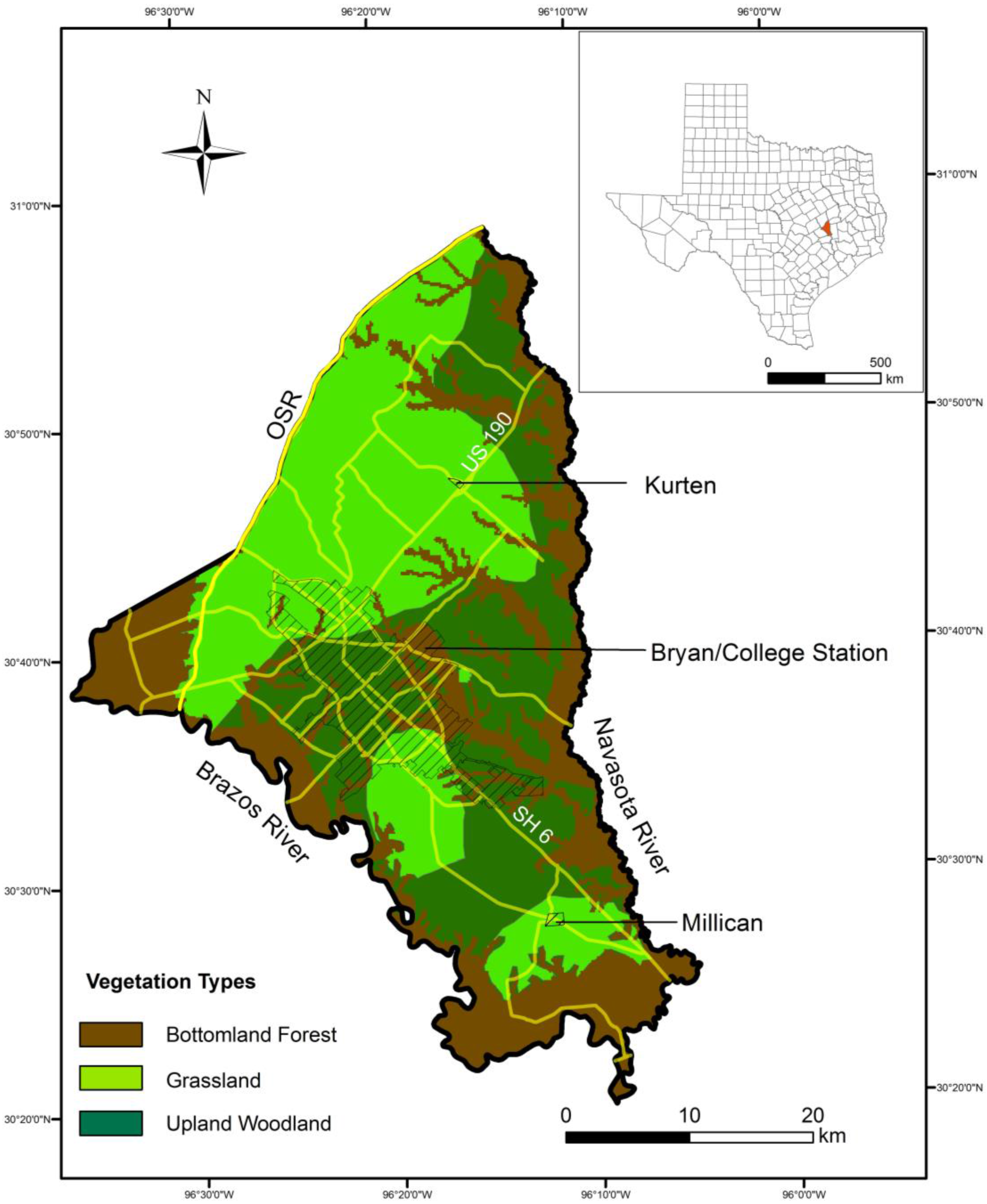
Spatially-Located Autecological InformationMapped Vegetation Classes
Bottomland ForestUpland WoodlandGrasslandRow Totals
Bottomland trees21813222
Upland trees169323011249
Open ground markers11125679
Column totals2459453601550
Overall map accuracy77.8%
Notes: The rows indicate the autecological point data corresponding to upland and bottomland trees and open ground locations derived from the surveyor’s notes. The number of items of autecological point data corresponding to the mapped classes are provided in each column: those in black are correctly located, those in blue are errors of commission and those in red errors of omission.
Twelve open ground sites were included in the upland woodland class. These inclusions can be explained by the fact that the two upland classes (prairie grassland and upland woodland) were likely a continuum from open grassland, through low-tree density wooded grassland to dense oak-dominated woodlands, not mutually exclusive vegetation assemblages. In ecological terms, the sharp boundary derived from the geostatistical analysis occurs within a dynamic ecotone in which trees and shrubs can encroach onto the grassland. However, this encroachment was probably controlled by fire and therefore some woodland-grassland boundaries could have been quite distinct.
Assuming the woodland-grassland boundary was broad rather than sharp, the commission and omission data in Table 3 can be explained in terms of assumptions about the behavior of the surveyors. In very sparsely wooded terrain and prairie grasslands surveyors would be unlikely to walk long distances to trees, even where they existed, when they could more easily mound up stones or earth, or hammer in a wooden stake. In more densely wooded savannahs they did not have to walk far to trees to undertake the preferred method of surveying using a witness tree. Tree densities lend support to this argument. They were calculated using the following equation:
D ( i ) = ( n = 0 n d ) / a ( i )
where D(i) is the tree density for vegetation cover i (trees ha−1), n is the number of trees in cover type i, d is the distance between the tree and survey point along the bearing line for each tree(m), and a(i) is the area of cover type i (ha).
Tree densities of 101 trees ha−1 for the bottomland forest, 19 trees ha−1 for the upland woodlands, and 5 trees ha−1 for the grasslands were calculated.
Furthermore is the fact that in upland woodlands there is only one percent error in grassland commission. Sixteen upland trees were misallocated to the bottomland forest class. Most of these are boundary errors involving Quercus stellata (13 trees) at the bottomland forest-upland woodland boundary. These misallocations may be due to surveying measurement errors or are trees at the extremes of their range of ecological tolerance.
Verification of historical vegetation and land cover is difficult. The Brazos County land surveys were completed before the routine use of photography in this area. Old photographs in local libraries date from the early 1900s and were mainly restricted to people and buildings. Nonetheless some were used for partial “verification” of the vegetation map, along with historical writings and by mapping the bottomland-upland (floodplain) topographic boundary in the contemporary landscape. Photographs dating from 1925 to 1930 from the area that is now Bryan/College Station show either extensive open grassland behind newly constructed buildings, or houses built in mature oak woodland. In all cases the vegetation in the photographs corresponded to the predicted vegetation type. Terraces and bluffs define the limits of the floodplains in Brazos County and a GPS survey conducted along these correlated well with the modeled bottomland-upland boundaries in Figure 1. Some early traveler’s letters lend general support to the reconstructed vegetation patterns [51]; for example, the following description of the forests along the Brazos River: “(The) Brazos bottoms are very wide and level, the trees are large and tall! (sic) the timber, renders the sight that is more imposing”.

5.2. Vegetation-Soil Relationships

Vegetation-site relationships have been a focus of presettlement vegetation reconstruction [27,28,29,30,31,32,33]. Interfluves in Brazos County are characterised by alfisols and vertisols with ustic soil moisture regimes. Usterts dominate the Blackland Prairie soil-ecological unit, while ustalfs dominate the Claypan Savannah and Claypan Prairie soil-ecological units. Uderts (vertisols with an udic soil moisture regime) dominate the floodplains, though alfisols (udalfs) form on sand-rich bars and levees. These are mapped as the Clayey and Loamy Bottomland soil-ecological units respectively on the USDA-NRCS maps for Brazos County.
Table 4 provides a contingency table of the relationships between reconstructed land cover (Figure 1) and the soil-ecological units. The proportional data were derived by overlaying Figure 1 on digital soil-ecological maps obtained from USDA-NRCS. Two soil-ecological units are important in that they describe unique vegetation cover-soil ecological units relationships in the presettlement vegetation. The Blackland Prairie only contained grasslands, while the Clayey Bottomlands unit only had bottomland forests. None of the reconstructed vegetation cover types was restricted to a single soil-ecological unit, though the majority of each cover type was found in one soil-ecological unit (Table 4). Almost three-quarters of grasslands were found in the Claypan Prairie unit, 81% of bottomland forests were found in the Clayey Bottomland unit and 84% of upland woodlands grew on Claypan Savannahs.
Table 4. The proportions of Upland Woodland, Bottomland Forest and Grassland in each soil-ecological unit determined by overlaying the map of reconstructed vegetation types (Figure 1) onto the soil-ecological units mapped in Brazos County by Natural Resources Conservation Service, US Dept. of Agriculture.
Soil Ecological Units
Blackland PrairieClaypan PrairieClaypan SavannahLoamy BottomlandClayey Bottomland
Soil typeUstertUstalfUderts and Udalfs
Proportion of Upland Woodland00.150.840.010
Proportion of Bottomland Forest00.010.010.160.81
Proportion of Grasslands0.120.740.110..010
When the autecological point data (i.e., trees labeled as upland or bottomland, and open ground markers) are examined in the context of soil-ecological units a slightly different picture emerges (Table 5). The majority of upland trees (75%) occurred in the Claypan Savannah, whereas over 90% of the bottomland trees were split almost evenly between the Clayey and Loamy Bottomlands units. Over 80% of grassland (open ground) locations occurred in the Claypan Savannah and Claypan Prairie units.
Table 5. The proportions of upland trees, bottomland trees and open ground locations in each soil-ecological unit. The proportions were determined by overlaying individual tree and open ground locations derived from surveyors’ records onto the soil-ecological units mapped in Brazos County by Natural Resources Conservation Service, US Dept. of Agriculture.
Autecological InformationSoil-Ecological Units
Blackland PrairieClaypan SavannahClaypan PrairieClayey BottomlandsLoamy Bottomlands
Upland (U) Trees (see Table 2)0.020.750.150.020.06
Bottomland (B) Trees (see Table 2)00.070.030.420.48
Grassland (Open Ground Locations)0.030.230.5900
Differences between vegetation cover and individual tree occurrences occur in both the bottomlands and uplands. In the former, the dominant bottomland forest-Clayey Bottomland association does not reflect the more even distribution of trees between both bottomland units, whereas in the uplands the cover proportions and tree occurrences are similar for the Claypan Prairie and Savannah units. Grassland cover and open ground markers vary slightly between three soil-ecological units. Reconstructed grassland cover is overrepresented compared with the occurrence of open ground markers in the Blackland and Claypan Prairie units, while the opposite is the case for the Claypan Savannah unit. These relationships lend support to earlier studies on prairies [56] and oak woodlands [57].

5.3. Vegetation Assemblages

Two vegetation assemblages were identified from the point autecological data for the reconstructed upland woodland and bottomland forest classes. The upland woodland species assemblage was dominated by Quercus stellata (88.9% of tree locations in the upland woodland class), with only three other species present—Quercus marilandica (10.4%), Quercus velutina and Juniperus virginiana (both <0.1%). The bottomland forest had higher taxon richness than the upland woodlands with 18 different types of tree, and was more diverse (Table 6). Despite the relatively high taxonomic richness, three species accounted for over 60% of trees—Quercus phellos (26.5% of the trees in the bottomland forests), Ulmus spp. (19.5%) and Carya illinoinensis (16.0%)—with Spanish Oak (7.3%), Fraxinus spp. (6.3%), Populus deltoides (5.1%), Quercus stellata (4.2%), Nyssa sylvatica, Quercus nigra (both 3.5%), Gleditsia triacanthos and Quercus lyrata (both 2.2%) accounting for approximately a third of the trees.
Table 6. Diversity metrics for Presettlement Upland Woodland and Bottomland Forests.
MetricUpland WoodlandBottomland Forest
Taxon richness418
Shannon’s H0.3792.202
Simpson Index0.8020.149
Scrifes [58] provides tree and shrub species information for Brazos County which can be used to compare with presettlement species composition. Extensive tracts of oak savannah woodland still exist in the south of the county. These mainly comprise Quercus stellata and Quercus marilandica canopies over a grass, herb and bare soil understory. However, in some areas there is a woody thicket understory dominated by Bumelia lanuginosa, Celtis pallida, Ilex vomitoria, Symphoricarpos orbiculatus, Ulmus alata and Vaccinium arboreum. None of these genera were recorded in the reconstructed upland tree assemblage, though Ulmus spp. has been recorded on upland tree-grassland associations in north Texas [37]. The absence of these genera is probably due to the fact that some species, e.g., Ilex vomitoria, are shrubby species that surveyors would have ignored particularly where there were abundant oaks to choose as witness trees.
Differences between the species composition of the Brazos and Navasota bottomland forests arise from differences in soil properties [59]. The Brazos bottomlands, with calcareous, moderately well drained chromuderts, were dominated by Celtis mollis, Populus deltoides and Quercus nigra. In comparison the acidic, poorly drained entic paleuderts along the Navasota and its tributaries were and still are dominated by Nyssa sylvatica, Quercus lyrata, Quercus macrocarpa and Spanish Oak.

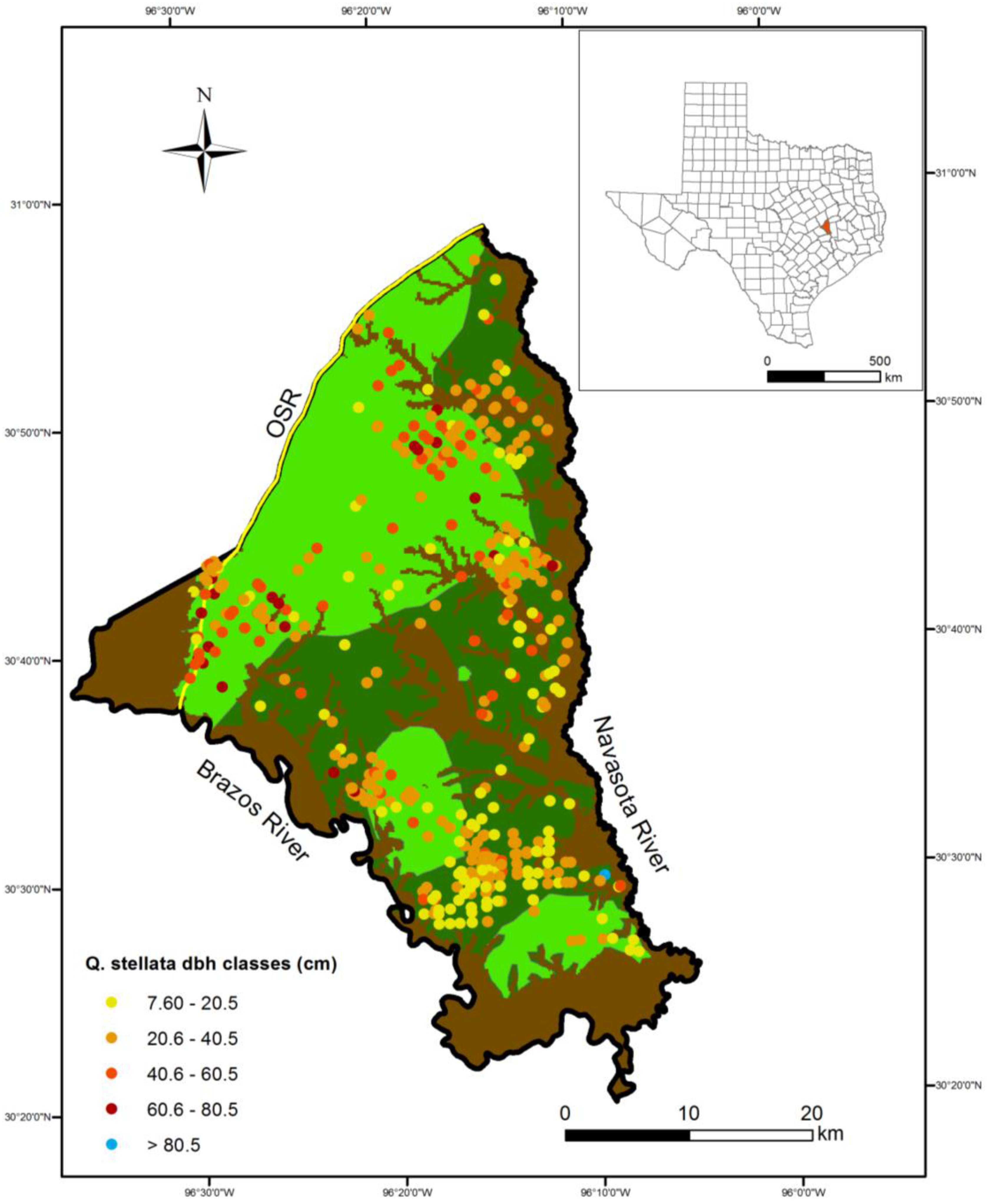
5.4. Tree Diameter Data

Tree diameter data for the five most frequently occurring species are provided in Table 7. The modal dbh for elms, Carya illinoinensis and Quercus marilandica was 20–40 cm, compared to 40–60 cm for Quercus phellos and 60–80 cm for Quercus stellata (Table 7). Quercus stellata and Quercus phellos were the only species with individuals in the >80 cm dbh class and were also the most frequently recorded trees in the >60 cm class.
Table 7. dbh data for the five most frequently occurring trees in the presettlement forests in Brazos County.
SpeciesNumber of Trees (Number with dbh Measurements in Parentheses)dbh Range (cm)Number of Trees by dbh Class (cm)
0–2020–4040–6060–80>80
Carya illinoinensis33 (38)10.2–76.21020120
Quercus marilandica134 (114)10.2–50.82387400
Quercus phellos83 (64)12.7–83.81039951
Quercus stellata1125 (976)7.6–91.453634215695
Ulmus spp.40 (55)7.6–66.01524010
Figure 2 maps the distribution of Quercus stellata by dbh class (Table 7) in the reconstructed vegetation classes. Almost all of the largest specimens (dbh > 60 cm) were located in the upland woodland class. Smaller trees were frequently found in the grasslands as well as the upland woodlands. While this would be expected given the broad ecotonal nature of this boundary in many parts of the county, because these data are skewed towards larger specimens of each species because of surveyor bias [42,60] there would have been oversampling of Quercus stellata as witness trees in grasslands. Mapping individual trees and the dbh data are therefore a useful way of lending support to the reconstructed vegetation class distributions and ecological interpretations, but can only be indicative of the upper limits of tree sizes under the natural conditions that prevailed in Brazos County in the mid 19th Century because of sampling biases.
Figure 2. Individual occurrences of Quercus stellata trees overlain on the presettlement vegetation map for Brazos County (Figure 1). The majority of the largest specimens (dbh > 60 cm) were located in the upland woodlands, while smaller specimens were more broadly represented in the grasslands and the upland woodlands. Very few specimens of this obligate upland tree were recorded in the bottomlands.
Land 05 00004 g002

6. Conclusions

The research clearly shows that OTLS data is well suited to the purpose of reconstructing and mapping presettlement vegetation cover in the Post Oak Savannah region of Texas. This supports earlier research [37,44,45] but most importantly provides evidence that quantitative analyses of OTLS data can add significantly to our knowledge of the land cover, vegetation and ecology at the time of settlement. The importance of this lies in the fact that (1) Texas was settled later than states to the east; (2) many settlers moved from the eastern United States to Texas and that, significantly, included Afro-American; and (3) the area spans a broad regional vegetation boundary comprising warm temperate mixed deciduous-hardwood forests to the east, through oak savannahs, to prairie grasslands. The Post Oak Savannah is the key biome in this regional boundary in the southern United States and reconstructing land cover is potentially important for regional environmental change studies in the southern Great Plains.
Acquiring OTLS data and converting it to geo-referenced autecological information is straightforward. The following analyses can be accomplished in a relatively straightforward manners: (1) reconstructing vegetation and land cover and mapping it; (2) conducting vegetation- and species-site analyses by spatially referencing these maps to soil-ecological units; and (3) constructing vegetation assemblages along with rudimentary analyses of forest and woodland structure. A major constraint is the ability to map the forest-grassland ecotone spatially. Figure 1 and Figure 2 show these as crisp boundaries, but ecological theory indicates that this may be incorrect. This occurs because of the problems of spatial extrapolation of irregularly spaced autecological point data and is more of an issue in the Post Oak Savannah biome that in many, but not all, forest reconstructions carried out in north-east and eastern North America.

Acknowledgments

This research was conducted while the authors worked at Texas A&M University. We gratefully acknowledge the help received from the Texas General Land Office; insightful comments from Clarissa Kimber, Fred Smeins, Charles Lafon, Srini Sriniwasan and Christian Brannstrom; and the support of the biogeography group in the Texas A & M Department of Geography, particularly Serena Aldrich and Will Flatley. Our thanks go also to Cécile Cutler for proofreading the manuscript.

Author Contributions

Research design: Indumathi Srinath (I.S.) and Andrew Millington (A.M.); data collection and spatial modeling (I.S.), map verification, ecological analysis and paper writing (I.S., A.M.).

Conflicts of Interest

The authors declare no conflict of interest.

References

  1. Forster, D.; Swanson, F.; Aber, J.; Burke, I.; Brokaw, N.; Tilman, D.; Knapp, D. The importance of land-use legacies to ecology and conservation. BioScience 2003, 53, 77–88. [Google Scholar]
  2. Phillips, J.D. Laws, contingencies, irreversible divergence and physical geography. Prog. Geogr. 2004, 56, 37–43. [Google Scholar]
  3. Brudvig, L.A.; Grman, E.; Habeck, C.W.; Orrock, J.L.; Ledvina, J.A. Strong legacy of agricultural land use on soils and understory plant communities in longleaf pine woodlands. For. Ecol. Manag. 2013, 310, 944–955. [Google Scholar]
  4. Ellis, E.C.; Goldewijk, K.K.; Siebert, S.; Lightman, D.; Ramankutty, N. Anthropogenic transformation of the biomes, 1700 to 2000. Glob. Ecol. Biogeogr. 2010, 19, 589–606. [Google Scholar] [CrossRef]
  5. Whitney, G.G.; DeCant, J. Government land office survey and other early land surveys. In The Historical Ecology Handbook: A Restorationist’s Guide to Reference Ecosystems; Egan, D., Howell, E.A., Eds.; Island Press: Covelo, CA, USA, 2001; pp. 147–172. [Google Scholar]
  6. Whitney, G.G. From Coastal Wilderness to Fruited Plain: A History of Environmental Change in Temperate North America, 1500 to the Present; Cambridge University Press: New York, NY, USA, 1996. [Google Scholar]
  7. Wang, Y.-C. Presettlement land survey records of vegetation: Geographic characteristics, quality and modes of analysis. Prog. Phys. Geogr. 2005, 29, 568–598. [Google Scholar]
  8. Maines, K.L.; Mladenoff, D.J. Testing methods to produce landscape-scale presettlement vegetation maps from the U.S. public land survey records. Landsc. Ecol. 2000, 15, 741–754. [Google Scholar] [CrossRef]
  9. Shanks, R.E. Forest composition and species association in the beech-maple forest region of western Ohio. Ecology 1953, 34, 455–466. [Google Scholar]
  10. McIntosh, R.P. The forest cover of the Catskill Mountain region, New York, as indicated by land survey records. Am. Midl. Nat. 1962, 68, 409–423. [Google Scholar] [CrossRef]
  11. Wuenscher, J.E.; Valinuas, A.J. Pre-settlement forest composition of the River Hills Region of Missouri. Am. Midl. Nat. 1967, 78, 487–495. [Google Scholar]
  12. Delcourt, H.R.; Delcourt, P.A. Presettlement magnolia-beech climax of the Gulf Coastal Plain: Quantitative evidence from the Apalachicola River bluffs, north-central Florida. Ecology 1977, 58, 1085–1093. [Google Scholar]
  13. Marks, P.L.; Gardescu, S. Vegetation of the central Finger Lakes region of New York in the 1790s. In Late Eighteenth Century Vegetation of Central and Western New York State on the Basis of Original Land Survey Records; Marks, P.L., Gardescu, S., Seischab, F.K., Eds.; New York State Museum: Albany, NY, USA, 1992; pp. 1–35. [Google Scholar]
  14. Schwartz, M.W. Natural distribution and abundance of forest species and communities in northern Florida. Ecology 1994, 75, 687–705. [Google Scholar]
  15. Cowell, C.M. Presettlement piedmont forests: Patterns of composition and disturbance in central Georgia. Ann. Assoc. Am. Geogr. 1995, 85, 65–83. [Google Scholar]
  16. Nelson, J.C. Presettlement vegetation patterns along the 5th principal meridian. Am. Midl. Nat. 1997, 137, 79–94. [Google Scholar]
  17. Dyer, J.M. Using witness trees to assess forest change in southeastern Ohio. Can. J. For. Res. 2001, 31, 1708–1718. [Google Scholar] [CrossRef]
  18. Cogbill, C.V.; Burk, J.; Motzkin, G. The forests of presettlement New England, USA: Spatial and compositional patterns based on town proprietor surveys. J. Biogeogr. 2002, 29, 1279–1304. [Google Scholar]
  19. Cox, L.E.; Hart, J.L. Two centuries of forest compositional and structural change in the Alabama Fall Line Hills. Amer. Midl. Nat. 2015, 174, 218–237. [Google Scholar]
  20. Lorimer, G.G. The presettlement forest and natural disturbance cycle of northeastern Maine. Ecology 1977, 58, 139–148. [Google Scholar]
  21. Grimm, G.C. Fire and other factors controlling the big woods vegetation of Minnesota in the mid-nineteenth century. Ecol. Monogr. 1984, 54, 291–311. [Google Scholar] [CrossRef]
  22. Whitney, G.G. Relation of Michigan’s presettlement pine forests to substrate and disturbance history. Ecology 1986, 67, 1548–1559. [Google Scholar] [CrossRef]
  23. Foster, D.R. Land-use history (1730–1990) and vegetation dynamics in central New England, USA. J. Ecol. 1992, 80, 753–772. [Google Scholar]
  24. Nelson, J.C.; Redmond, A.; Sparks, R.E. Impacts of settlement on floodplain vegetation at the confluence of the Illinois and Mississippi Rivers. Trans. Ill. State Acad. Sci. 1994, 87, 117–133. [Google Scholar]
  25. Batek, M.J.; Rbertus, A.J.; Schroeder, W.A.; Haithcoat, T.L.; Compass, E.; Guyette, R.P. Reconstruction of early nineteenth-century vegetation and fire regimes in the Missouri Ozarks. J. Biogeogr. 1999, 26, 397–412. [Google Scholar]
  26. Zhang, Q.; Pregitzer, K.S.; Reed, D.D. Catastrophic disturbance in the presettlement forests of the upper peninsula of Michigan. Can. J. For. Res. 1999, 29, 106–114. [Google Scholar] [CrossRef]
  27. Black, B.A.; Abrams, M.D. Analysis of temporal variation and species-site relationships of witness tree data in southeastern Pennsylvania. Can. J. For. Res. 2001, 31, 419–429. [Google Scholar] [CrossRef]
  28. Siccama, T.G. Presettlement and present forest vegetation in northern Vermont with special reference to Chittenden County. Am. Midl. Nat. 1971, 85, 153–172. [Google Scholar]
  29. Whitney, G.G. Vegetation-site relationships in the presettlement forests of northeastern Ohio. Bot. Gaz. 1982, 143, 225–237. [Google Scholar]
  30. Whitney, G.G.; Stieger, J.R. Site-factor determinants of the presettlement prairie-forest border areas of north-central Ohio. Bot. Gaz. 1985, 146, 421–430. [Google Scholar] [CrossRef]
  31. Leitner, L.A.; Dunn, C.P.; Cuntenspergen, G.B.; Stearns, F. Effects of site, landscape features and fire regime on vegetation patterns in presettlement southern Wisconsin. Landsc. Ecol. 1991, 5, 203–217. [Google Scholar]
  32. Barrett, L.R.; Liebens, J.; Brown, D.G.; Schaetzl, R.J.; Zuwerink, P.; Cate, T.W.; Nolan, D.S. Relationships between soils and presettlement forests in Baraga County, Michigan. Am. Midl. Nat. 1995, 134, 264–285. [Google Scholar]
  33. Abrams, M.D.; McCay, D.M. Vegetation site relationships of witness trees (1780–1856) in the presettlement forests of eastern West Virginia. Can. J. For. Res. 1996, 26, 217–224. [Google Scholar]
  34. Sears, P.B. The natural vegetation of Ohio. I. A map of the virgin forest. Ohio J. Sci. 1925, 25, 139–149. [Google Scholar]
  35. Texas Parks and Wildlife Department. The Vegetation Types of Texas; Texas Wildlife and Parks Department: Austin, TX, USA, 1984. [Google Scholar]
  36. Rodgers, C.S.; Anderson, R.C. Presettlement vegetation of two prairie Peninsula counties. Bot. Gaz. 1979, 140, 232–234. [Google Scholar] [CrossRef]
  37. Jurney, D.H. General land office surveys: Mapping the presettlement prairie landscape. In Proceedings of the 10th North American Prairie Conference, Denton, TX, USA, 22–26 June 1986.
  38. Dyer, J.M.; Baird, P.R. Remnant forest stands at a prairie ecotone site: Presettlement history and comparison with other maple-basswood stands. Phys. Geogr. 1997, 18, 146–159. [Google Scholar]
  39. Cowell, C.M.; Jackson, M.T. Vegetation change in a forest remnant of the eastern presettlement prairie margin, USA. Nat. Areas J. 2002, 22, 53–60. [Google Scholar]
  40. US Army Corps of Engineers. Regional Supplement to the Corps of Engineers Wetland Delineation Manual: Atlantic and Gulf Coastal Plain Region (Version 2.0); ERDC/EL TR-10-20; US Army Corps of Engineers: Vicksburg, MS, USA, 2010. [Google Scholar]
  41. Correll, C.M.; Johnson, M.C. Manual of the Vascular Plants of Texas; University of Texas Press: Austin, TX, USA, 1979. [Google Scholar]
  42. Srinath, I.S. Original Texas Land Survey as a Source for Pre-European Settlement Vegetation Patterns. Master’s Thesis, Texas A & M University, College Station, TX, USA, December 2009. [Google Scholar]
  43. Jacobson, P. The evolution of Texas land surveys. In Presented at the AM/FM/GIS Conference, Dallas, TX, USA, 29 October 1992; 1992. [Google Scholar]
  44. Schafle, M.P.; Harcombe, P.A. Presettlement vegetation of Hardin County, Texas. Am. Midl. Nat. 1983, 109, 355–366. [Google Scholar]
  45. Wills, F.H. Structure of historic vegetation on Kerr wildlife management area, Kerr County, Texas. Texas J. Sci. 2002, 57, 137–152. [Google Scholar]
  46. Reasonover, J.R.; Haas, M.M. Reasonover’s Land Measures; Copano Bay Press: Copano Bay, TX, USA, 2005. [Google Scholar]
  47. Jordan, T.G. Antecedents of the Long-Lot in Texas. Ann. Assoc. Am. Geogr. 1974, 64, 7–86. [Google Scholar] [CrossRef]
  48. Srinath, I.; Millington, A.C. Reconstructing Texan land cover using historical land survey data. In Progress in Geospatial Science Research; Arrowsmith, C., Bellman, C., Cartwright, W., Jones, S.D., Shortis, M., Eds.; School of Mathematical and Geospatial Science, RMIT University: Melbourne, Australia, 2011; pp. 270–287. [Google Scholar]
  49. Gammel, H.P.N. The Laws of Texas; Gammel Book Company: Austin, TX, USA, 1898. [Google Scholar]
  50. United States Department of Agriculture. Plants Database. Available online: http://plants.usda.gov/ (accessed on 11 November 2015).
  51. Dewees, W.B. Letters from an Early Settler in Texas; Texan Press: Waco, TX, USA, 1968. [Google Scholar]
  52. Burrough, P.A. Natural objects with indeterminate boundaries. In Geographic Objects with Indeterminate Boundaries; Burrough, P.A., Frank, A.U., Eds.; Taylor and Francis: London, UK, 1996; pp. 3–28. [Google Scholar]
  53. Wang, Y.-C.; Larsen, C.P.S. Do coarse resolution U.S. presettlement land survey records adequately represent the spatial pattern of individual tree species? Landscape Ecol. 2006, 21, 1003–1017. [Google Scholar]
  54. Texas State Library and Archives Commission (1979–). Old San Antonio Road Preservation Commission. Available online: http://www.lib.utexas.edu/trao/10198/tsl-10198.html (accessed on 15 March 2013).
  55. Jordan, T.G. Pioneer evaluation of vegetation in frontier Texas. Southwest. Hist. Q. 1973, 76, 223–254. [Google Scholar]
  56. Smeins, F.E.; Diamond, D.D. Remnant grasslands of the Fayette Prairie, Texas. Am. Midl. Nat. 1983, 110, 1–13. [Google Scholar] [CrossRef]
  57. Johnston, F.L.; Risser, P.G. Some vegetation-environment relationships in the upland forests of Oklahoma. J. Ecol. 1972, 60, 655–663. [Google Scholar]
  58. Scifres, C.J. Brush Management. Principles and Practices for Texas and the Southwest; Texas A & M University Press: College Station, TX, USA, 1980. [Google Scholar]
  59. Smeins, F.E.; Texas A&M University, College Station, TX, USA. Personal communication, 2010.
  60. Hanberry, B.B.; Yang, J.; Kabrick, J.M. Adjusting forest density estimates for surveyor bias in historical Tree surveys. Am. Midl. Nat. 2012, 167, 285–306. [Google Scholar]

