Article

Investigating Impacts of Alternative Crop Market Scenarios on Land Use Change with an Agent-Based Model

1
Department of Geographical and Sustainability Sciences, University of Iowa, 316 Jessup Hall, Iowa City, IA 52242, USA
2
Esri, 380 New York Street, Redlands, CA 92373, USA
3
Department of Geography and Environmental Resources, Southern Illinois University, Carbondale, IL 62901, USA
*
Author to whom correspondence should be addressed.
Land 2015, 4(4), 1110-1137; https://doi.org/10.3390/land4041110
Submission received: 1 January 2015 / Revised: 9 November 2015 / Accepted: 16 November 2015 / Published: 24 November 2015
(This article belongs to the Special Issue Agent-Based Modelling and Landscape Change)

Abstract

:
We developed an agent-based model (ABM) to simulate farmers’ decisions on crop type and fertilizer application in response to commodity and biofuel crop prices. Farm profit maximization constrained by farmers’ profit expectations for land committed to biofuel crop production was used as the decision rule. Empirical parameters characterizing farmers’ profit expectations were derived from an agricultural landowners and operators survey and integrated in the ABM. The integration of crop production cost models and the survey information in the ABM is critical to producing simulations that can provide realistic insights into agricultural land use planning and policy making. Model simulations were run with historical market prices and alternative market scenarios for corn price, soybean to corn price ratio, switchgrass price, and switchgrass to corn stover ratio. The results of the comparison between simulated cropland percentage and crop rotations with satellite-based land cover data suggest that farmers may be underestimating the effects that continuous corn production has on yields. The simulation results for alternative market scenarios based on a survey of agricultural land owners and operators in the Clear Creek Watershed in eastern Iowa show that farmers see cellulosic biofuel feedstock production in the form of perennial grasses or corn stover as a more risky enterprise than their current crop production systems, likely because of market and production risks and lock in effects. As a result farmers do not follow a simple farm-profit maximization rule.

1. Introduction

Midwestern landscapes are dominated by commodity crops including corn, soybean, and wheat. Commodity prices and the policies affecting them are the key drivers of farmers’ decisions about agricultural practices, such as crop rotations and fertilizer rates. Federal and state policies on renewable energy production interact with commodity markets to affect decisions about changes in crop type and land management. These decisions, in turn, have significant environmental impacts in terms of water quantity and quality, soil erosion, and carbon sequestration in the Midwest [1,2,3,4]. Farmers’ involvement in the production of biofuel crops (e.g., corn stover, miscanthus, and switchgrass) could result in new land use patterns and, thus, altered environmental outcomes. Due to substantial risk associated with the adoption of novel agricultural practices, however, farmers may not follow the same maximum profit rules when considering biofuel crop production as they do when considering traditional crops. To achieve insight into the potential impact of biofuel crop markets on agriculture land use, empirical information about farmers’ attitudes towards novel practices must be integrated into land use models.
Secchi et al. [5] investigated the potential water quality changes associated with market scenarios of decreasing soybean to corn price ratio in the Upper Mississippi river basin by integrating an economic-driven land use model and the Soil and Water Assessment Tool (SWAT), a surface water quality model. Their results showed that an increase in corn acreage by 14.4% could result in increase in N loadings to the watershed by 5.4% and P loadings by 4.1%. Another similar study was conducted to investigate the impacts of different corn price scenarios on crop rotation patterns and environmental consequences in Iowa, USA, by integrating an economic model and the edge of field environmental impact model EPIC (Environmental Policy Integrated Climate) [6]. The authors found that sustained high corn prices might result in continuous corn in crop rotation patterns on both current cropland and CRP (Conservation Reserve Program) land. This change in land management is associated with increased sediment and nitrogen loss from fields to surface water. Leaving crop residues such as corn stover in field can help recycle nutrients, control surface runoff and prevent water and wind erosion. Potential biofuel markets for corn stover feedstock could force further shifts from corn-soybean rotation to continuous corn and a significant reduction of crop residue, thus, creating further losses of soil, nitrogen (N) and phosphorus (P) [7]. As an alternative, switchgrass, a native perennial grass in the Midwest, has been extensively investigated as a potential feedstock for cellulosic biofuel production. Switchgrass is currently used in riparian buffer strips to reduce sediment, N and P in surface runoff [8], however, its production as a biofuel crop requires the use of fertilizers that can make their way to surface and groundwater [9].
Various approaches, such as statistical techniques, expert models (e.g., Bayesian probability), cellular models (cellular automata and Markov models), and hybrid models that combine multiple techniques have been applied in land use modeling [10]. These approaches, however, focus mainly on spatiotemporal patterns of land use change rather than the decision-making process of individual land managers, despite the fact that these managers are the essential driving force in the complex land use dynamics [11].
Agent-based model (ABM) is a computer simulation approach that can be used for land use modeling [10,12]. Agent-based land use models represent system complexity using a bottom-up approach that characterizes the decision making processes of heterogeneous agents as well as feedback processes among agents and between agents and the biophysical environment. Simulated agents, such as land owners, ranchers, farmers, and policy makers, act and interact following decision rules. They are characterized by sets of parameters that can be derived from theory or empirical data obtained by land use surveys, participatory observations, and field and laboratory experiments [13,14]. Due to the mechanistic nature of this approach and its unique perspective concerning agent-agent and agent-environment interactions, ABMs are often integrated with environment models to explore the impacts of socio-economic driving forces or alternative policies on land use and consequent environment outcomes [15,16,17]. ABM can be used to represent multiple types or levels of agents (e.g., institutions and individuals) and the co-evolution of and interaction between biophysical and human decision making processes in a coupled human-environment system [10,18,19,20,21,22].
In Midwestern agricultural landscapes, ABM has been applied in studies on how farmer decision making is impacted by agricultural policies, such as the CRP [23], potential market scenarios of biofuel crops [24], and price incentives for nitrogen and carbon abatement [25,26]. In the first two studies [23,24], the research is focused on how land use changes emerge from farmers’ decisions under the assumption that the natural environment is static through time. In the latter two studies [25,26], the focus is on the impacts of farmers’ management decisions on water quality. The authors integrated ABM with SWAT, and analyzed two-way interactions between farmer agents and the natural environment. The natural environment included two types of processes: biological and hydrological, both of which interacted with agents but at different levels. Agents’ decisions on cropping practices not only influenced but also responded to crop yields. Agents’ decisions affected watershed water quality, but there was no feedback from water quality into the agents’ decisions. The study was considered as “semi-hypothetical” since no empirical information was used to parameterize agents’ risk premiums towards novel agricultural practices.
The research objectives of this study are to: (1) develop an ABM to simulate farmers’ decisions about land use practices given a risk-averse profit maximization rule; and (2) investigate the impacts of alternative market scenarios on land use change by integrating empirical information about farmers’ attitudes into an ABM. Through this study, we address the following research questions: (1) is the current land cover pattern economically optimal given declines in crop yield resulting from continuous corn/soybean rotation? and (2) would biofuel crops be underutilized given farmers current attitudes towards biofuel crop production?

2. ABM of Agricultural Land Use

2.1. Mathematical Programming for Modeling Decision Making in ABM

Farm household modeling often relies on mathematical programming (MP) techniques to simulate land management decision of farmers and their responses to policy. This approach has several drawbacks [12,23]: (1) it generally assumes the maximization of a single objective (e.g., profit), which is often not appropriate when modeling the adoption of new technologies; (2) it ignores the social aspects of farm households such as communication and interaction among farmers in the same community; and (3) it does not properly capture the heterogeneity of the social behaviors and responses of farmers. In ABMs of agricultural land use decision making, mathematical programming is generally applied at the farm level and combined with heuristic approaches and Bayesian inference or Bayesian probability networks [23,25,26,27]. Heuristic approaches, such as decision trees or rule-based models, assume limited human cognition, while optimization approaches, such as MP, assume that inefficiency in human decisions comes from external factors, such as the failure of institutions, imperfect markets, and lack of infrastructure or limited information [27]. Though the two approaches appear to be different in theory, Schreinemachers and Berger [27] argue that in practice they can be converted into each other. For example, decision rules about production and consumption in heuristic approaches can be incorporated into MP models as constraints. An optimization approach is even more appropriate for policy analysis and planning since it can quantitatively characterize the outcomes of alternative policies.
In the Midwestern U.S., Sengupta et al. [23] employed a hybrid approach to model land enrollment in an agricultural land set aside conservation program, CRP. Different types of farmers with distinct decision making rules were modeled in the Cache River watershed of southern Illinois. In another example of ABM for agricultural land use, Ng [25] and Ng et al. [26] combined a farm-level stochastic programming model with a Bayesian updating procedure to represent the optimization and adaption processes of farmers’ decision in the Salt Creek watershed in Central Illinois. In Ng’s ABM [25,26], the farmers are assumed to be economically rational with bounded information. Farmer agents learn new information through time with Bayesian updating. In this ABM, farmers interact with their geographic neighbors to exchange information about crop yields and costs.

2.2. Empirical Information for ABM
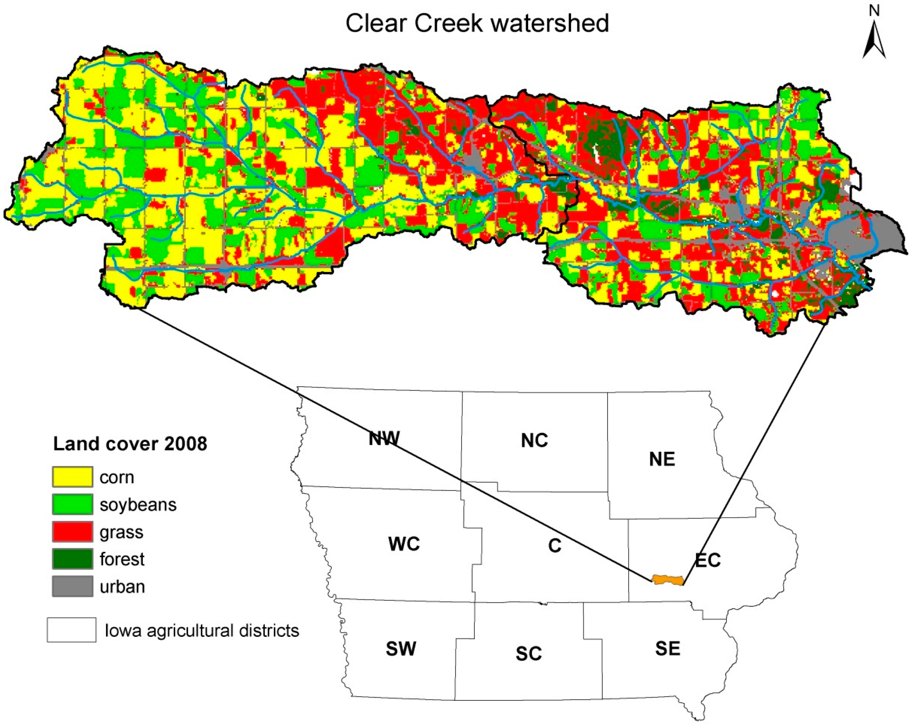
Empirically-based ABMs for land use simulation construct and parameterize decision making models from empirical information that characterizes macro-level patterns and micro-level processes. Information about micro-level processes could be directly utilized for developing and testing the structure of decision making models in ABM, while datasets about macro phenomena are usually applied in calibrating and validating the model [13]. In this study, we focus mainly on empirical information about micro-level processes and its use for the parameterization of the decision making model.
To characterize heterogeneous agents and their behavioral responses, empirical information needs to be analyzed using statistical methods (e.g., factor or cluster analysis, regression) and GIS techniques. Based on the statistical descriptions of agents characteristics derived from observation datasets, different populations of unique artificial agents can then be generated with Monte Carlo techniques [28].
Smajgl et al. [14] developed a framework for generating and calibrating the parameters that describe agent attributes and behavioral functions. In their framework, the parameterization process is composed of five steps: (1) create an agent typology based on behavioral differences; (2) specify the attribute values for each agent type; (3) specify the behaviors of each agent type by obtaining the parameter values for their behavioral functions; (4) develop agent types from agent attributes or behavior responses; and (5) generate a population(s) of agents based on the agent typology, and relevant attributes and parameters.
Empirical information can be collected using various methods [10,13,14]. These methods include role-playing games [29,30], sample surveys [31], participatory observations [32], field or laboratory experiments [33], and GIS and RS data collection [34]. Of these five methods, sample survey is the most quantitative approach and can be carried out at a relatively large spatial scale [13]. Though qualitative information about agents’ interactions and feedbacks could be obtained using different methods, it is still challenging to empirically identify and quantify social, spatial and cross-scale interactions among agents and feedbacks between agents’ decisions and the biophysical processes [35].

3. Study Area

The study area is the Clear Creek watershed located in Iowa and Johnson Counties in Eastern-Central Iowa, U.S. (Figure 1). It is a typical Midwestern agricultural watershed dominated by row crops (corn, soybean), with an area of about 267 km2. The average annual temperature from 2000 to 2011 was 10 °C and average annual precipitation was 886 mm based on the weather records at the Iowa City Municipal Airport station. According to the United States Department of Agriculture National Agricultural Statistical Services (NASS) remote sensing Cropland Data Layer (CDL) images in 2008, the percentages of the predominant cover types were respectively 29.77% corn, 20.11% soybean, and 28.17% grassland/pasture. Additionally, 14.56% of the total watershed was in urban and developed uses and 6.9% was forest including deciduous, evergreen and mixed forest. Urban and forest areas are located mainly in the eastern part of the watershed. According to the Iowa Soil Properties and Interpretations Database (ISPAID), about 54% of the watershed is covered by soil with slope range of 2%–14%; while soils are distributed among several soil drainage type ranging from well drained soils (26%), moderate-well drained soils (23.5%), to poorly drained soils (11.9%). The dominant soil textures of the surface horizon in the region are silty clay loam (35.8%) and silt loam (35.1%); about 45% of the total land is highly erodible.
Figure 1. The Clear Creek Watershed in East-Central Iowa.
Land 04 01110 g001
According to an agricultural land use survey conducted in 2010 [36,37], the dominant crop rotation type is corn-soybean and corn-corn-soybean with conventional tillage used for both corn and soybean. Some farmers adopt conventional tillage practices for corn but no-till or minimum-till practices for soybean. Specific information about actual application rates of inorganic N fertilizers in corn fields is not available for this watershed. According to Iowa State University Extension [38], the highest N rate is applied for corn after corn (168–224 kg/ha), followed by corn after soybean if no manure is applied (112–168 kg/ha), and corn on recently manured soils (0–101 kg/ha), given that all N is applied before corn planting or crop emergence.

4. Model Description

In this section, the model is described following the Overview, Design concept and Details (ODD) protocol [39].

4.1. Overview

4.1.1. Purpose

This model is used to simulate farmers’ decisions on agricultural land use including crop type, tillage type, and fertilizer rates. We aim to run simulations to study farmers’ decisions on biofuel crop productions in response to biofuel crop prices.

4.1.2. Entities, State Variables, and Scales

Agents in the model are farmers. Each farmer agent corresponds to a farm composed of one or more land parcels that are represented by command land units (CLUs) in this study. Farmer agents have attributes including farm size, and parameters about their attitudes towards biofuel crop production are summarized in Table 1.
We use eight parameters to characterize farmers’ responses to the questions in Table A1 and thereby to describe their attitudes towards biofuel crop production and the associated risk premium. Descriptions of the eight parameters are included in Table 1. Additionally, there is a parameter Area representing the land acreage of the farm size of each farmer agent.
Each land parcel has attributes including area (in hectares), Corn Suitability Rate (CSR) (dimensionless) which is an index of land suitability for crop production, and potential yield of switchgrass (metric ton/ha).
Based on each land unit, farmer agents make CLU-specific decisions on crop type, tillage type, and fertilizer rates by changing the value of the CLU-specific (i as index) and year-specific (t as index) state variables: Xi, j, t, and j represents all available options for crop type, tillage type, and fertilizer rate levels. Xi, j, t is a binary variable about crop type, tillage type, and N application rate level. Crop types include corn (with or without stover harvest), soybean, and switchgrass. Tillage types include conventional tillage, mulch tillage, and no tillage. Fertilizers include N, P, and K (potassium). For example, Xi, j=1, t = 1 means corn is planted in land parcel i at year t, Xi, j=2, t = 1 means soybean is planted in land parcel i at year t, and Xi, j=3, t = 1 means the land parcel i is fallow at year t. Similarly, j = 4 6 X i , j , t = 1 and j = 4, 5, 6, respectively, mean conventional tillage, mulch tillage, and no tillage. When j = 7, 8, …, 16, Xij is the decision variable of the N application level from the lowest to the highest. In the biofuel crop market scenarios, crop type decision variables also have two extra options, switchgrass, and corn with stover harvested.
Table 1. Parameters characterizing farmers’ attitudes towards biofuel crop production.
ParameterValueAgent Characteristics
Type0Not interested in either marketing corn stover or planting switchgrass
1Only interested in marketing corn stover
2Only interested in planting switchgrass
3Interested in both
Profit SWGNumericProfit rate ($/ha) required by the farmer to plant, harvest and market switchgrass *
Percent1 SWGNumericPercent of farm acreage on which the farmer would plant switchgrass if the Profit SWG can be achieved
Percent2 SWGNumericPercent of farm acreage on which the farmer would plant switchgrass if 1.5 times the Profit SWG can be achieved
Profit StvrNumericProfit rate ($/ha) required by the farmer to harvest and market corn stover *
Percent1 StvrNumericPercent of farm acreage on which the farmer would consider harvesting and marketing corn stover if the Profit Stvr can be achieved
Percent2 StvrNumericPercent of farm acreage on which the farmer would harvest, and market corn stover if 1.5 times the Profit Stvr can be achieved
Portion StvrNumericPortion of corn stover that the farmer would harvest
* Given that in 2010 when the survey was conducted, the average price for corn was $196.85/metric ton and for soybean was $404.14/metric ton).
One simulation step represents one year. Farmer agents make decisions on each land parcel (CLU) of their farms every year. CLUs are the smallest land units with common crop choice and management, a continuous boundary and the same owner and operator. Thus, in the ABM, land parcels represented as CLUs are the smallest simulation units for which both the physical conditions (soil fertility, slope, etc.) and farmer’s land use management practices are assumed to be homogeneous. Generally, a farm is composed of multiple CLUs and each farm corresponds to a single land use decision maker represented as a farmer agent in the ABM. Data for CLU boundaries in Iowa are available to the public through the Natural Resources Geographic Information Systems (NRGIS) Library. However, the information about farm boundaries is confidential and thus cannot be publically displayed. In this study, we generate pseudo farm boundaries by utilizing the statistical distribution of farm sizes, and the spatial locations of farm centroids based on real information of farm boundaries.

4.1.3. Process Overview and Scheduling

Each year, farmer agents estimate commodity prices and fuel prices, calculate crop production costs and returns, and make decisions on crop type, tillage type, and fertilizer rates. To make these decisions, farmer agents try to maximize farm profit given the constraints of crop yield drag effect, and their risk aversions towards biofuel crop production.
More specifically, at each time step, for each farmer agent, the land use decision making process is implemented in two parts in the model. In Part I, linear programming is used to look for land use practices that maximize farm profit with planning horizon of 1 year given the crop choices of corn without stover, soybean and fallow. The 1-year planning horizon is used in biofuel crop market scenarios. In model verification, 1-year, 2-year, and 3-year planning horizons are used. In Part II, a decision-tree based algorithm is designed for comparing the profit rates determined from Part I with the profit rate from corn with stover at the simulation step, and with the average yearly profit rate from corn with stover and switchgrass calculated within a 10-year planning horizon (discount rate = 0.05). If the risk premium for biofuel crops is met and expected profits exceed those of traditional crops, the profit maximizing biofuel crop will be selected and planted. Total biofuel production is limited by farm specific acreage constraints. For next time step, the same two processes are implemented except that the land parcel that was previously enrolled in switchgrass is be excluded from the farm profit maximization until it is out of the 10-year enrollment limit.

4.2. Design Concepts

4.2.1. Principles

We assume that farmers are risk averse profit maximizers, and that there is little risk associated with the choice between corn and soybeans, since they are both well-established annual crops. Therefore, in the case of these crops the decision rule collapses to profit maximization. However, there is substantial risk associated with new markets and crops. Further, if these crops are perennials, they lock in farmers for substantial periods of time, thereby increasing both market and production risk.
In all cases, farm profit depends on yield potential for corn, soybean, and switchgrass specific to each land parcel. Corn and soybean yields are lower if the crops are not rotated, and corn yield responds to different levels of N rates. Because of the additional risk associated with cellulosic ethanol markets, farmer agents might require higher profits from biofuel crops than they do from traditional crops and limit the total acreage allocated to biofuel crops.

4.2.2. Emergence

Watershed-scale agricultural land use acreages and fertilizer application rates are modeled as an emergent property of farmer agent decisions. For model results, we expect to observe insensitivity of cropland switched to switchgrass and corn stover harvest in response to the price change due to farmers’ risk aversions towards biofuel crop production.

4.3. Details

4.3.1. Initialization

We use NASS CDL data from 2001 to 2011 for initializing the land cover in the first two years of simulation and compare with the simulation results in the remaining years. NASS CDL is a raster data set at 30 meter spatial resolution. It contains land cover information of specific crop types including corn and soybean. We use the majority zonal operator in ArcGIS 10.0 to aggregate the pixel-specific crop type into the CLU level.

4.3.2. Input Data

The ABM inputs include prices and land parcel information. The price file contains annual time series of prices for crops (corn, soybean, switchgrass, corn stover), fertilizers (N, P, K), and fuels (diesel, LPG-liquid petroleum gas). The parcel information file contains land parcel specific data about acreage, CSR, yield potential for switchgrass, and land cover types for the previous two years. These data were used to construct net returns for each field in the watershed for each crop rotation [6]. In addition, a parameter file characterizing farmer agents’ attitudes towards biofuel crop production (as in Table 1) is a necessary input into this model. The price data was based on United States Department of Agriculture’s (USDA’s) Economic Research Service, U.S. Energy Information Administration and Iowa State University Extension’s budgets [38,40,41], the CSR data was obtained from the soil database ISPAID, the historical landcover was constructed using the CDL, and the attitudes of farmers were parameterized from a land use and attitudes survey conducted in 2010 [36,37].

4.3.3. Submodels

As mentioned, there are two parts of the decision making processes. In Part I, for current iteration year, the farm based objective function is:
m a x i m i z e   P = i = 1 n ( S i C i )
where i is the land parcel index, n is the total number of land parcels within a farm, P is the profit, S is revenue from crop sale, and C is crop production cost. Equation (1) illustrates that the farm agents’ objective is to maximize farm profit each year. With decision variables included, Equation (1) can be expressed as:
m a x i m i z e   P = i = 1 n j = 1 m f ( c i j X i j )
where cij is the objective function coefficient corresponding to the jth variable for land parcel i, and Xij is the jth decision variable for land parcel i, n is the total number of land parcels within a farm, and m is the total number of decision variables. As illustrated in Equation (2), the farm profit maximization for corn and soybean is a linear programming problem, which is scripted in the mathematical programming software (AIMMS) and implemented as an ABM using C++.
After the implementation of Part I, the decision variable values and the resulting profit rates from the AIMMS optimization component are passed to the decision-tree based algorithm in Part II. In this part, profit rates for biofuel crops (corn with stover harvest, and switchgrass) are evaluated with the agent-specific risk premiums and compared to commodity crop profit rates obtained from the Part I algorithm. The biofuel crop is chosen for a land parcel when the risk premium for biofuel crops is met and expected profits exceed those of traditional crops. Empirical parameters characterizing farmers’ risk premiums about biofuel crops are incorporated in the decision-tree based algorithm. The parameters are derived from the land use survey and applied in the land use decision rule for switchgrass and corn stover production. The parameters and the sampling strategy of parameter values derived from the land use survey database are described in Table 1 and the Appendix B.

5. Data and Simulation Settings

5.1. Agricultural Landowners and Operators Survey

A survey of agricultural landowners and operators in the Clear Creek watershed was conducted in 2010 to obtain information about current farming practices and farmers’ willingness to participate in conservation practices and biofuel crop production [36,37]. The survey questions were sent by mail to all non-urban landowners and agricultural operators (about 998) within the watershed. Responses were received from 397 of them (response rate 41.1%). A survey database was developed based on those responses. The database covers multiple topics including personal information, farm characteristics, and farmers’ information sources and their attitudes towards watershed conservation and growing biofuel crops. For this study, we are interested in questions about (1) farm size; (2) minimum net profit rates that farmers require from biofuel crop production; (3) the acreage on which farmers would plant, harvest, and market corn stover and/or switchgrass; and (4) the proportion of corn stover harvested if such profits were realized (Table A1 in the Appendix B).

5.2. Price Scenarios and Simulation Settings

Price inputs to the model include commodity prices of corn, soybean, corn stover, switchgrass, fertilizers (N, P, K) and fuels (LPG and diesel). In this study, we run the ABM simulations with four different input datasets for commodity and biofuel crop prices to investigate: (1) the land use pattern resulting from profit maximization (Simulation Set I); (2) the sensitivity of land use pattern to commodity crop prices (Simulation Set II); (3) the impacts of biofuel crop prices on land use patterns given the risk associated with biofuel crop production (Simulation Set III, and Simulation Set IV).

5.2.1. Historical Market Prices

Simulation Set I is based on historical market prices from 2003 to 2011 (Table 2). The corn and soybean prices are the average prices in the calendar year (ISU cash corn and soybean prices) [42]. From 2003 to 2006, corn prices are replaced with the target prices of the counter-cyclical payments for corn. The fertilizer prices are the average U.S. farm prices of selected fertilizers in March or April published by USDA’s Economic Research Service. The LPG price is the weekly Iowa propane residential price in the middle of March and the diesel price is the price of Midwest No. 2 diesel retail sales by all sellers. The data is published by the U.S. Energy Information Administration.

5.2.2. Price Scenarios for Corn and Soybean

Simulation Set II (Table 3) is based on price scenarios for 360 combinations of corn prices and soybean prices. By confining the price ranges within the historical records and the ten year baseline projections for U.S. agricultural markets by the Food and Agricultural Policy Research Institute, University of Missouri (FAPRI-MU) [43], we determine 24 levels of corn prices and 15 levels of soybean to corn price ratios (Table 3). The 24 levels of corn price start from 360 (24 × 15) combinations of corn price and the price ratio are used for generating price inputs into the model. For the 360 price input files, the other prices including switchgrass, corn stover, fertilizers (N, P, and K), and fuels (diesel and LPG) are held constant. Switchgrass and corn stover are not taken into account and so their prices are considered as zero. Prices of fertilizers and fuels are the average values of FAPRI-MU projections.
Table 2. Historical market prices (corn, soybean switchgrass and corn stover prices in $/metric ton, fertilizer prices in $/kg, fuel prices in $/liter, soybean to corn price ratio is dimensionless).
YearCornSoybeanSwitch GrassCorn StoverNPKDieselLPGSoybean to Corn Ratio
2003102.36 *223.38000.410.270.180.380.292.18
2004103.54 *281.06000.420.290.200.440.282.71
2005103.54 *216.03000.460.330.270.560.332.09
2006103.54 *203.91000.570.360.300.750.391.97
2007132.68285.84000.580.460.310.730.402.15
2008188.19417.00000.830.880.621.160.562.22
2009150.00369.60000.750.700.940.570.432.46
2010151.97362.26000.550.560.560.800.462.38
2011234.65458.88000.830.700.661.060.491.96
* Corn prices are replaced with the target prices of the counter-cyclical payments according to the Farm Security and Rural Investment Act of 2002.
Table 3. Price levels of alternative scenarios (corn and soybean prices in $/metric ton, switchgrass and corn stover prices in $/metric ton, fertilizer prices in $/kg, fuel prices in $/L, price ratios are dimensionless).
Simulation SetNumber of CombinationsCornSoybeanSoybean: Corn Price RatioSwitchgrassCorn StoverSWG: Stvr Price RatioNPKDieselLPG
II360Start = 102.36 To = 283.46 Step = 7.9 (24 levels)Corn price × SC price ratio (15 levels)Start = 1.8 To = 3.2 Step = 0.1 (15 levels)00 0.890.800.761.030.48
III16186.6419.942.25Start = 58.41, To = 223.71, Step = 11 (16 levels)SWG price/SS price ratio (16 levels)1.310.890.800.761.030.48
IV96186.6419.942.25Start = 58.41, To = 223.71, Step = 11 (16 levels)SWG price/SS price ratio (6 levels)Start = 1.1, To = 2.1, Step = 0.2 (6 levels)0.890.800.761.030.48

5.2.3. Price Scenarios for Switchgrass and Corn Stover

Simulation Set III (Table 3) is based on 16 levels of switchgrass prices. By referring to the projected prices of warm season grasses and corn stover for biofuel markets by FAPRI-MU [44], we determine 16 levels of switchgrass prices from 58 $/metric ton to 224 $/metric ton with an interval of 11 $/metric ton. The price ratio of switchgrass to corn stover is fixed as 1.31 according to the average value in FAPRI-MU (2011). The other price inputs for corn, soybean, fertilizers and fuels are fixed as the average prices for Year 2012 to 2021 in the FAPRI-MU projections. In Simulation Set III, simulations are run for each of the 16 price levels with the 30 samples of the empirical parameter set. The model is run for a total of 480 (16 × 30) simulations. The last set of simulations (Simulation Set IV) (Table 3) uses the same price settings as Simulation Set III except that the price ratio of switchgrass to corn stover varies from 1.1 to 2.1 with interval of 0.2 (a total of 6 levels) Therefore, in Simulation Set IV, price scenarios are 96 (16 × 6) combinations of switchgrass and corn stover prices. Similarly to Simulation Set IV, simulations are run for each of the 96 combinations with 10 samples of the empirical parameter set. The model is run for totally 960 (96 × 10) simulations.

6. Results and Discussions

6.1. Model Verification

The yield drag incorporated in the ABM model on the basis of agronomic data effectively precludes the choice of continuous corn for the simulated farmers. Thus, farmers are de facto constrained to think in terms of corn-soybeans or corn-corn-soybeans in the model. In practice farmers may not behave as if the yield drag matters, which is verified by the crop rotation pattern comparison below.

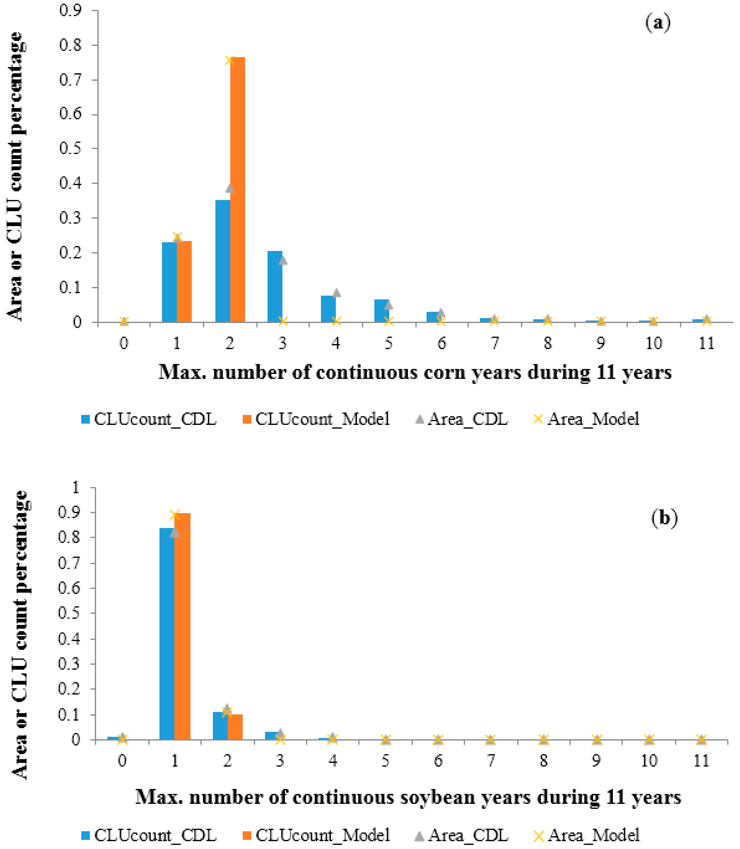
6.1.1. Crop Rotation Pattern

Figure 2 compares the simulated crop rotations with the NASS CDL based crop rotations using graphs that summarize the land area percentage and the CLU count percentage corresponding to the maximum number of continuous crop years during the 11-year time period. In Figure 2a, we see that about 74% of the simulated land is in corn-corn-soybean and about 26% of land is in corn-soybean during any of the 11 years. In reality, however, less land is in corn-corn-soybean (about 39%) while about the same percentage of land (25%) is in corn-soybean; and there are some fields (about 36%) which were in continuous corn for three or more years. For soybean (Figure 2b), the simulated and real landscapes are very similar: Single-year soybean is predominant (more than 80%). This indicates that in reality farmers do not necessarily follow the rotation patterns of corn-corn-soybean or corn-soybean, and that the continuous corn years could be longer than two, but soybean is grown almost always only in rotation with corn.
Assuming the NASS CDL is reality, we can conclude the inclusion of yield drag in the model and the likely underestimate of the effect of yield drag by actual farmers causes the model to underestimate the amount of continuous corn, because simulated farmers are in practice restricted in their options. For example, after two years of corn a simulated farmer will plant soybeans even if relative crop prices suggest that corn is the more profitable crop because of the effects of yield drag on productivity. Yield drag is, however, hard for actual farmers to ascertain because they do not run long term controlled experiments in their fields, many factors change simultaneously from year to year, and yield drag is affected by tillage and weather. Unfortunately, though there is anecdotal evidence [45,46] that farmers may underestimate yield drag, there are no peer-reviewed studies that compare perception and reality on this issue.
Overall though, the model gives a reasonable approximation of the behavior of farmers in the watershed for the study period. For example, the average acreage of cropland in corn according to the CDL dataset was 56.7% and the simulated average using the one year planning horizon was 52.2%. Again, the underestimation of corn acreage is related to the yield drag issue.
Figure 2. Maximum number of continuous corn (a); and soybean (b) years during an 11-year time period.
Land 04 01110 g002

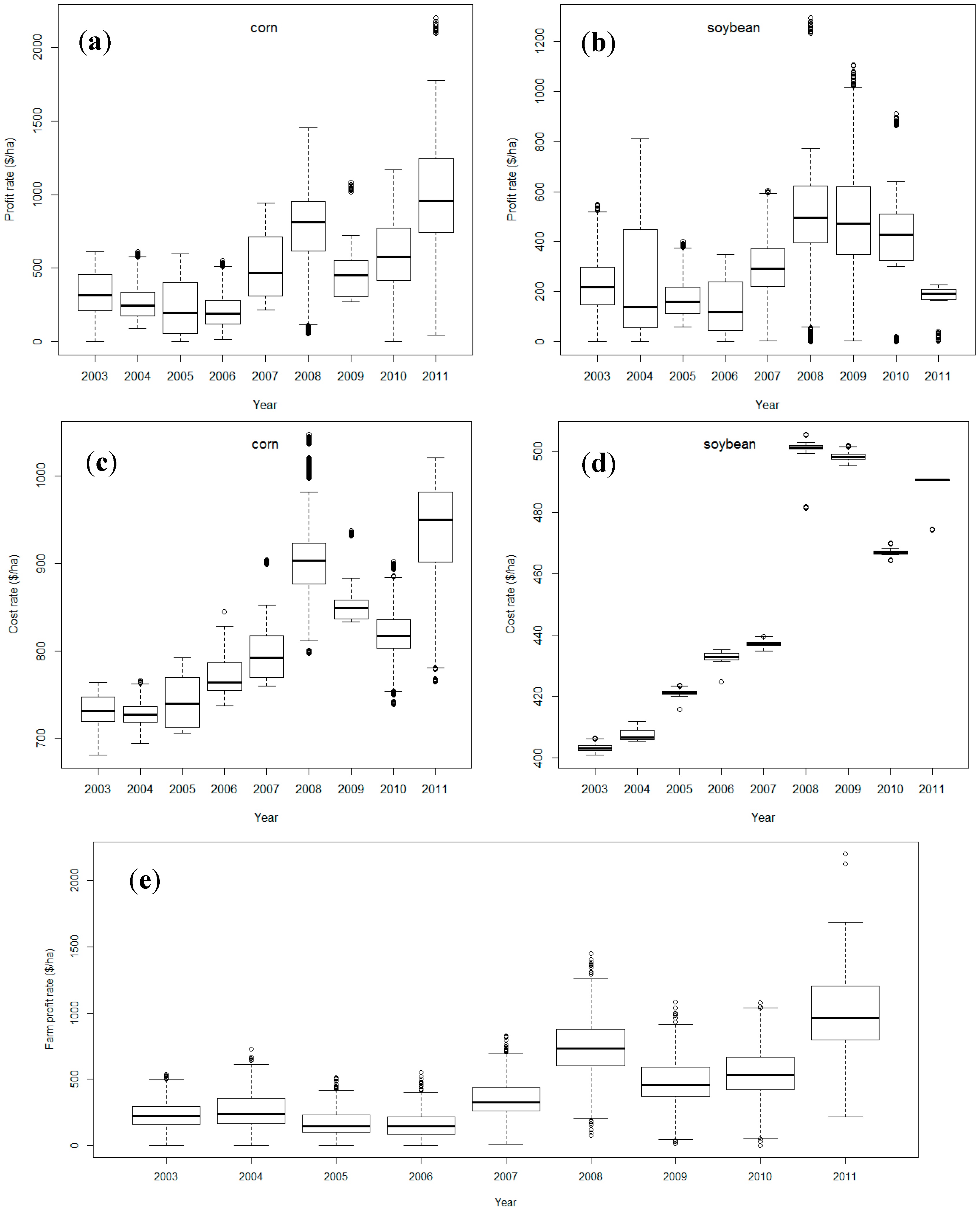
6.1.2. Field and Farm Scale Statistics

At the field scale, box plots are made for the cost and profit rates of corn and soybean throughout the 11 simulation years (Figure 3a–d). Generally, the simulated cost and profit rates increase through the years, and corn (Figure 3a,c) has higher cost and profit rates than soybean (Figure 3b,d). The box heights are generally larger in Figure 3c than Figure 3d, which indicates that the spatial variability (across fields) of the simulated cost rate of corn is much higher than soybean. The reason is that nitrogen fertilizer is only applied for corn and the N application rate varies across different corn fields depending on the physical characteristics of land (e.g., yield potential). At the farm scale, a box plot is made for the simulated profit rate over all simulation years (Figure 3e). The simulated average net farm income rates from 2008 to 2011 is about 694 $/ha, which is comparable to the overall average of typical cash rents from 2008 to 2011 for corn and soybean fields (respectively 460, 477, 484, and 541 $/ha) in the corresponding agricultural district (District 6) in Iowa [47]. The lower cash rent is likely due to the fact that cash rent is generally built as the average of recent past net returns and therefore lags.
Figure 3. Box plots of simulated profit rate ((a) corn; (b) soybean); and cost rate ((c) corn; (d) soybean); and of farm-level profit rate (e).6.2. Model Results: Corn and Soybean Price Scenarios (Simulation Set II).
Land 04 01110 g003
With the second set of simulation results, we plotted watershed-scale crop area percentages (Figure 4a,b) and fertilizer rates (Figure 4c,d) against changes in corn price and soybean to corn price ratio. As illustrated by Figure 4a, the percent of land in corn increases as corn price increases and/or as the ratio of soybean to corn price decreases. The percent of land in soybean changes with the opposite trends (Figure 4b). Corn and soybean lands stabilize at 50/50 within the corn price range of about 181.1–283.5 $/metric ton and the range of soybean to corn price ratio of about 2.8–3.2. Beyond this range, the percent of the landscape in corn and soybean is very sensitive to changes in corn price and/or soybean to corn price ratio.
Figure 4. Simulated crop area percentage ((a) corn; (b) soybean); and fertilizer rates averaged over the whole watershed ((c) N; (d) P; (e) K) for 360 combinations of corn prices and soybean to corn price ratios.
Land 04 01110 g004
According to Figure 4c, nitrogen responds to the changes in corn price and soybean to corn price ratio in a very similar way to corn acreage since N fertilizer is only applied for corn. The shape of the P surface is more similar to the corn land percentage surface than to the soybean, except that the lowest value of the average P application rate occurs when corn price is at the lowest (181.1 $/metric ton) and soybean to corn price ratio is at the lowest (2.8). This is because the average P application rate is related to both corn and soybean planting but dominated by corn since corn requires more P input than soybean. Figure 4e characterizes the response of K application rate to changes in corn price and the soybean to corn price ratio. The K surface has a shape more similar to that of the percent of the land in soybean than to corn, except that the lowest value of the average K application rate occurs at the same position as P. This is reasonable because the average K application rate is related to both corn and soybean planting but dominated by soybean since soybean requires more K input than corn. Within similar ranges (181.1–283.5 $/metric ton corn prices, and 2.8–3.2 of soybean to corn price ratio), the average N, P, and K rates stabilize respectively at around 65, 56, and 71 kg/ha.

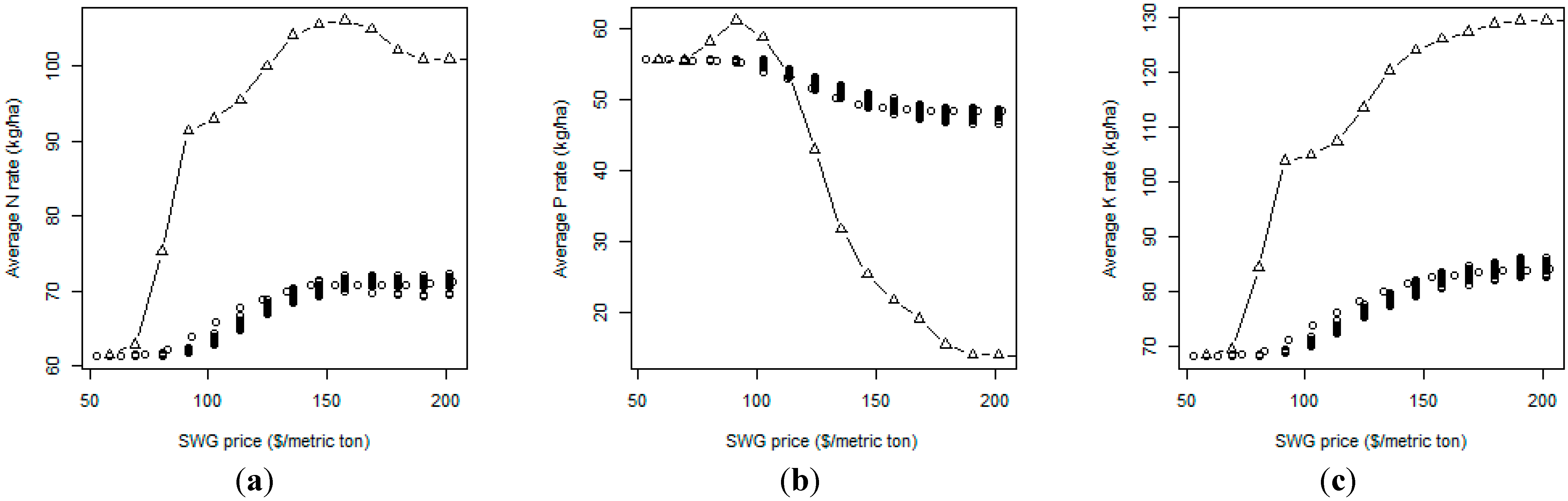
6.2. Model Results: Switchgrass and Corn Stover Price Scenarios

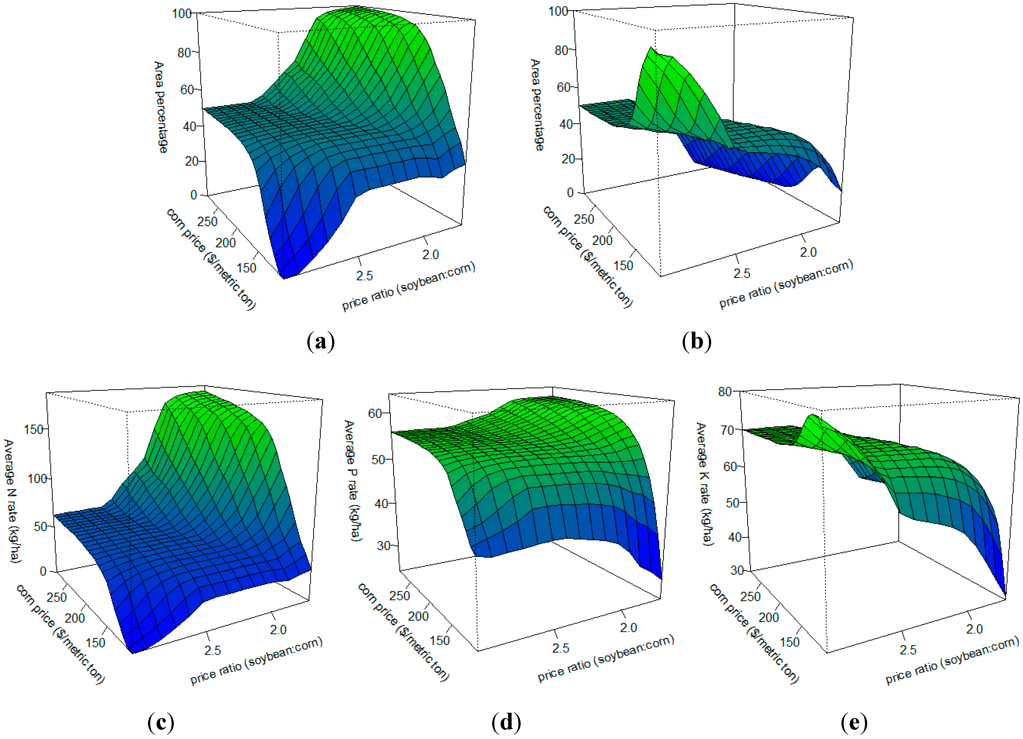
6.2.1. Simulations with vs. without Land Use Survey Information Included (Simulation Set III)

We run the model with positive switchgrass prices as defined in Simulation Set III under two scenarios:
Scenario 1. The agricultural landowners and operators survey information is not included in the model, and agents do not appreciate that there is additional risk in planting perennial crops for a new market. In this scenario farmer agents follow the same rule of farm profit maximization as they do in Simulation Set I (profit maximization unaffected by farmer risk perception);
Scenario 2. Information from the farmer survey is incorporated into the model and used to parameterize the perceived risks associated with planting a new perennial crop. In this scenario, agent-specific constraints are incorporated into the model which stipulate the minimum expected economic return required before a farmer would consider biofuel crops and the maximum percent of their farm they would allocate to biofuel crop production if such returns could be realized.
As illustrated in Figure 5, the incorporation of farmer attitudes about risk has a significant impact on land use. Considerably more land is allocated to switchgrass and corn stover in scenario 1 (profit maximization, triangles in Figure 5) than in scenario 2 (constrained by perceived risk, circles in Figure 5). Even with 30 simulations for each of switchgrass price levels, the variations are low (in Figure 5, the dispersion of 30 circles is small compared to the discrepancy between the circles and triangles). Figure 5a–d shows that when perceived risk is modeled, the simulated crop composition starts to change at switchgrass price of $88.16/metric ton (switchgrass to corn stover ratio fixed at 1.31) and above: Corn (no stover) (Figure 5a) and soybean (Figure 5b) acreages start to decrease and switchgrass (Figure 5c) and corn (stover) (Figure 5d) start to increase. The crop area percentage curves approach a stabilization stage at switchgrass prices of about 132–165 $/metric ton. The crop composition stabilizes at about 32% corn (no stover), 38% soybean, 22% switchgrass, and 8% corn (stover).
Figure 5. Crop area percentages ((a) corn—no stover; (b) soybean; (c) switchgrass; (d) corn—stover) from 36 simulations (36 SWG price levels and fixed switchgrass to corn stover price ratio of 1.31) on the basis of with (dots) vs. without (triangles in dashed line) land use survey information included.
Land 04 01110 g005aLand 04 01110 g005b
Similarly, there is a large discrepancy in simulated watershed level fertilizer application rates between scenario 1 and 2 (Figure 6). The variation of the fertilizer rates with scenario 2 given 30 random samples from the empirical distribution is small. Under scenario 2 the simulated N and K curves are sigmoid shaped while the P curve mirrors the sigmoid shape. As the switchgrass price increases within a certain range, the average N rate and K rate increase while the average P rate decreases. This is reasonable because P rate for switchgrass is relatively low compared to corn (stover or no stover) and soybean.
Figure 6. Watershed-averaged fertilizer rates ((a) N; (b) P; and (c) K) from 36 simulations (36 SWG price levels and fixed switchgrass to corn stover price ratio of 1.31) on the basis of with (dots) vs. without (triangles in dashed line) land use survey information included.
Land 04 01110 g006
The two runs in Simulation Set II correspond to the commodity crop price settings in Simulation Set III, corn price is 186.6 $/metric ton and the price ratio of soybean to corn is 2.25. The two runs are (1) corn price is 181.1 $/metric ton, and the soybean to corn price ratio is 2.4; and (2) corn price is 188.98 $/metric ton, and the soybean to corn price ratio is 2.24. Considering the two runs in Simulation Set II as baseline scenarios, the watershed-average N rate in Simulation Set III (ranging from 62.77 to 71.14 kg/ha) is higher than in the baseline (between 60.53 and 62.77 kg/ha). So is the watershed-average K rate in Simulation III (ranging from 67.25 to 84.07 kg/ha) compared to the baseline (68.37 kg/ha). The watershed-average P rate in Simulation III (ranging from 47.08 to 56.04 kg/ha) is lower than in the baseline (56.04 kg/ha). These results show that biofuel crop markets may potentially result in more N and K inputs and less P inputs into the watershed. This is understandable because (1) in the baseline scenario, corn-soybean rotation only needs N input in corn years, while once enrolled in switchgrass planting, it requires N input every year; (2) switchgrass requires more K input than corn and soybean do. Since switchgrass potentially has beneficial effects of reducing nutrient and sediment runoff [48,49] while commodity crops management and harvesting corn stover may have adverse effects [50], it would therefore be very interesting to investigate the impacts of potential biofuel crop markets on watershed water quality in a further study.

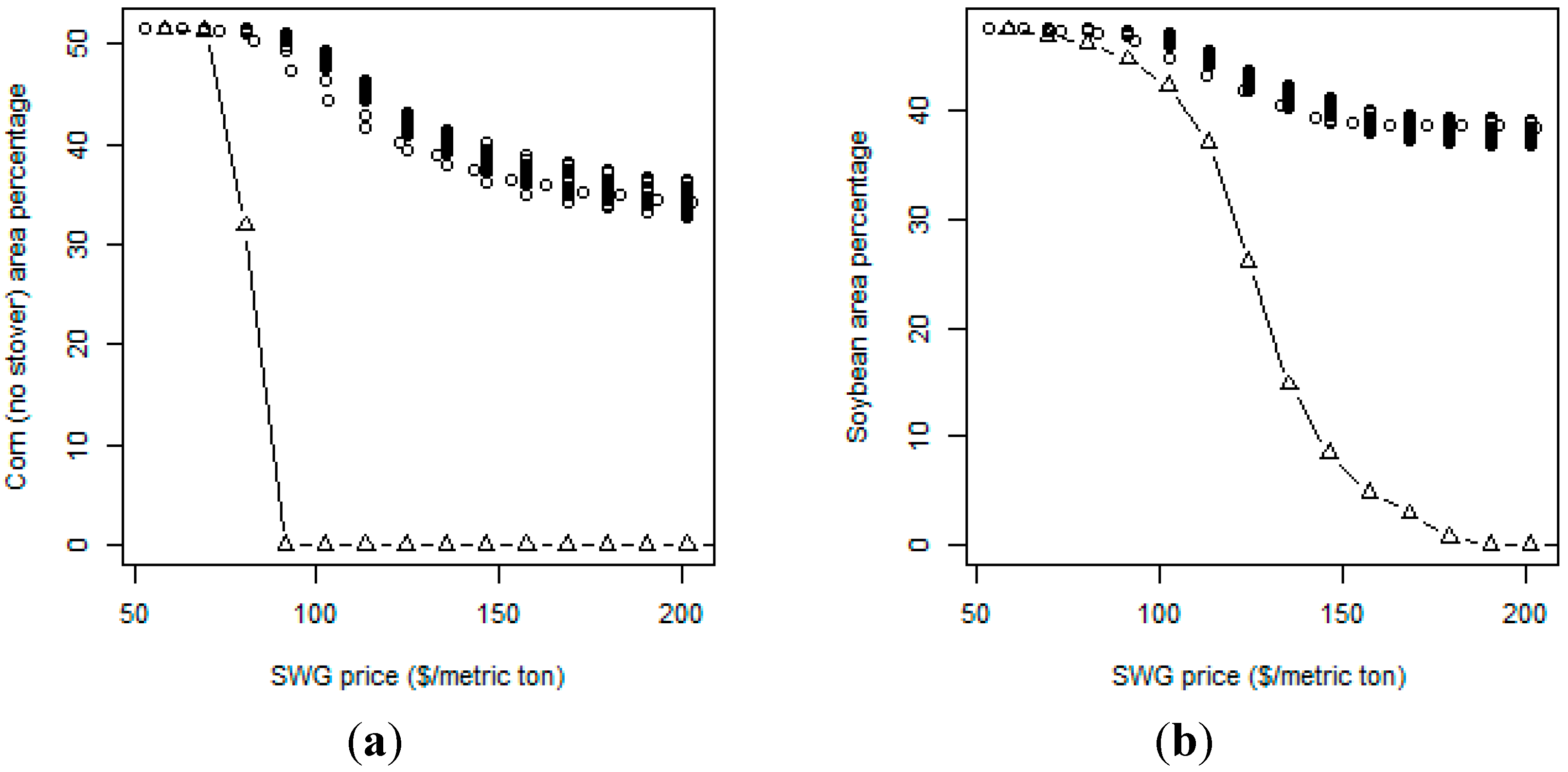
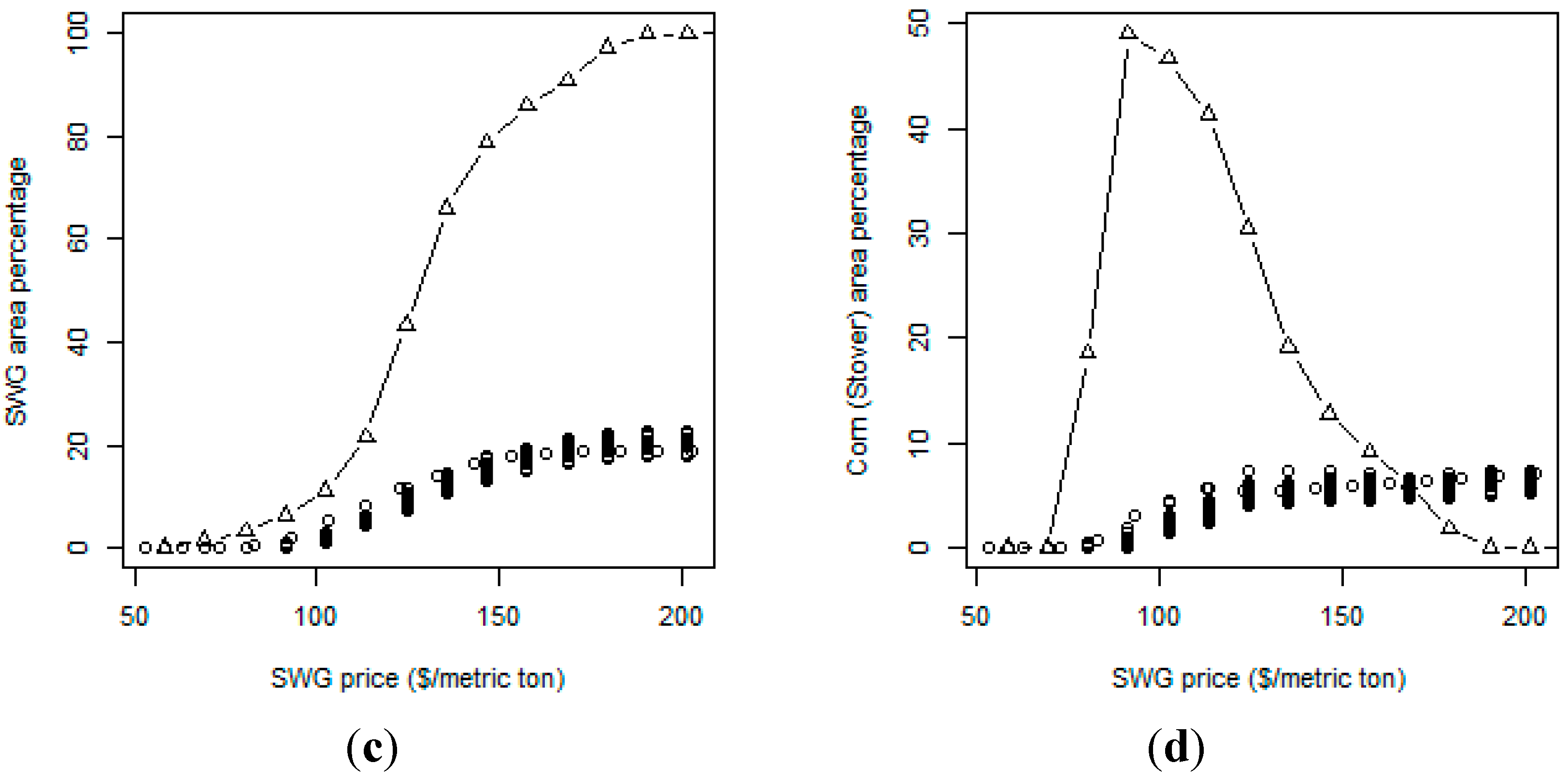
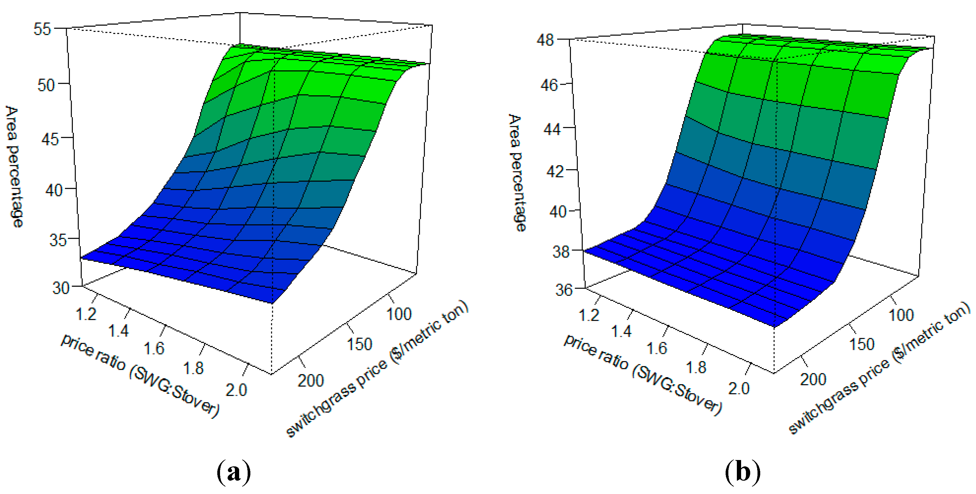
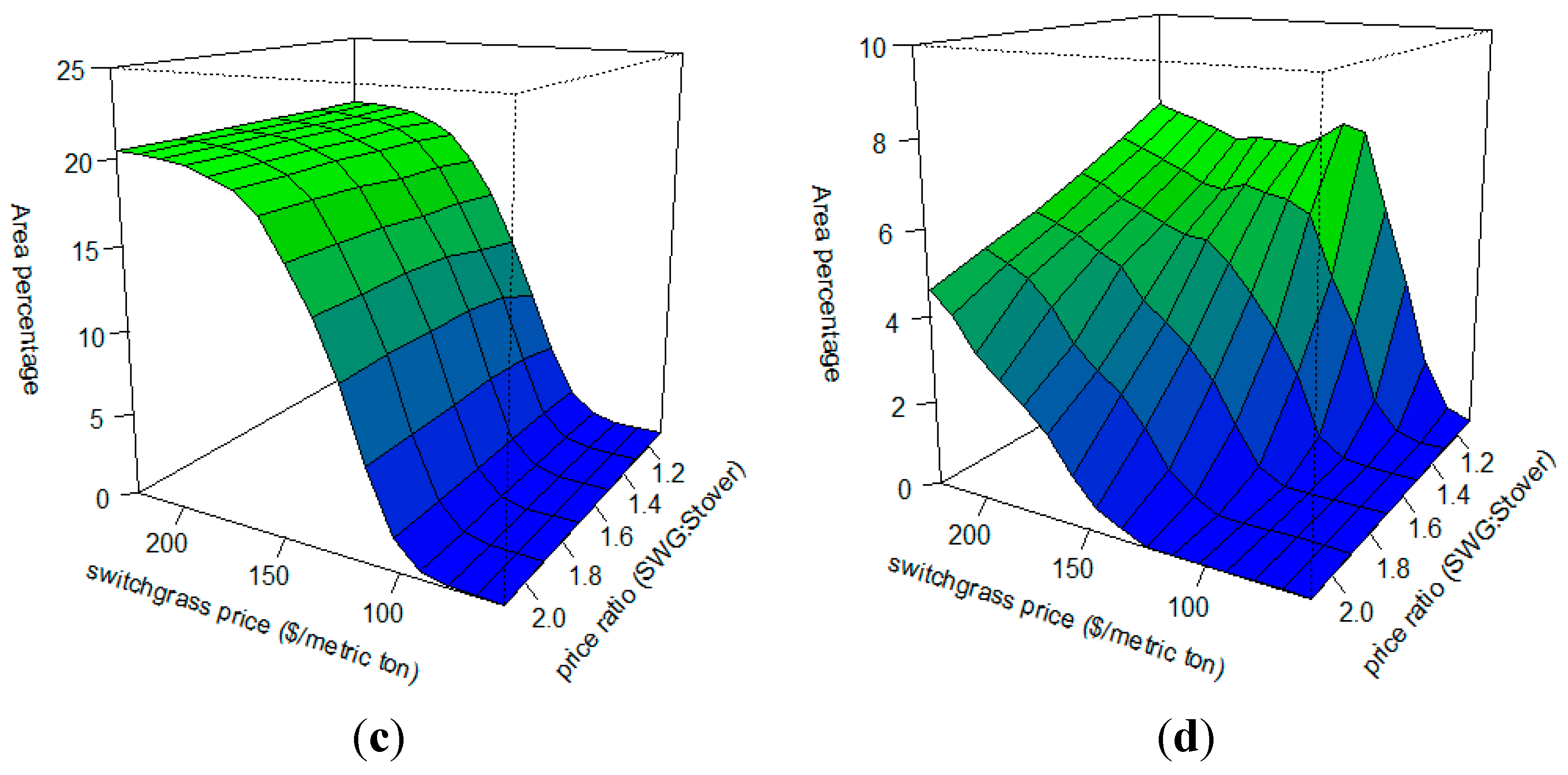
6.2.2. Impacts of Corn Stover and Switchgrass Price (Simulation Set IV)

In Simulation Set IV, both the switchgrass price and the price ratio of switchgrass to corn stover vary. Switchgrass price varies from 58.41 $/metric ton to 223.71 $/metric ton, and the price ratio of switchgrass to corn stover varies from 1.1 to 2.1. For each combination of the two variables, we run the simulation 10 times and plotted the average of the 10 as a response “surface” (Figure 7 and Figure 8).
Figure 7c,d shows that within the price ranges in Simulation Set IV, switchgrass occupies at most about 22%–24% of the watershed and corn stover occupies at most 10%. These numbers are consistent with those in Simulation Set III. In Figure 7a–d, at any fixed ratio of switchgrass: Corn stover (1.1–2.1), the crop area percent responds similarly to the curves represented by circles in Figure 6a–d except for corn (stover). At any fixed ratios greater than about 1.4, the corn (stover) area percentage curve does not stabilize within the switchgrass price range from 58.41 to 223.71 $/metric ton. Instead, it still keeps increasing even at the very high switchgrass price of 223.71 $/metric ton.
Figure 7. Crop area percentages ((a) corn—no stover; (b) soybean; (c) switchgrass; (d) corn—stover) from 960 simulations (16 levels of switchgrass price by 6 levels of switchgrass to corn stover price ratio, average of the 10 random samples based simulations for each combination).
Land 04 01110 g007aLand 04 01110 g007b
Figure 8. Watershed-averaged fertilizer rates ((a) N; (b) P; and (c) K) from 960 simulations (16 levels of SWG price by 6 levels of switchgrass to corn stover price ratio, average of the 10 random samples based simulations for each combination)
Land 04 01110 g008
Overall, the crop area percentage in Figure 4a,b (corn and soybean scenarios) responds more rapidly to the change of price ratio than in Figure 7a–d (switchgrass and corn stover scenarios). We may conclude that the price ratio of switchgrass to corn stover does not influence the crop composition as much as the price ratio of soybean to corn.
In Figure 8a–c, we plotted watershed-averaged N, P, and K rates in response to the change of switchgrass prices and switchgrass to corn stover price ratios. Similarly to Figure 6a–c, the watershed-averaged N and K rates increase as switchgrass prices increase but the watershed-averaged P rate decreases as switchgrass prices increase. N, P, and K rates stabilize, respectively, at 67.25–73.98 kg/ha, 44.83–49.32 kg/ha, and 81.82–87.43 kg/ha when switchgrass price reaches 132.24–165.3 $/metric ton and higher. The fertilizer rates in the switchgrass-corn stover scenarios (Figure 8a–c) respond more rapidly to the change of switchgrass price than to the change of price ratio. At fixed level of switchgrass price, fertilizer rates hardly respond to the change of switchgrass to corn stover ratio within the range of 1.1 to 2.1.

7. Conclusions

The major findings in this research include: (1) discrepancies exist between simulated and satellite-derived land acreages and crop rotation patterns, with implications in terms of farmers’ estimation on crop yield drag effects; (2) the simulated biofuel crop land acreage response surface starts to plateau at prices beyond $150/ton for switchgrass; and (3) simulated biofuel crop land acreages and fertilizer application rates in response to alternative crop market scenarios differ significantly depending on whether or not the risk averse behavior of farmers towards biofuel crop production is considered. These findings help define the decision space for future biofuel production, and provide insights for different stakeholders, such as agricultural policy makers who are concerned about commodity and biofuel crop land use and inputs of fertilizer into the agricultural system. Since currently no crop insurance is available for biofuel crops, our results also indicate the importance of creating such a program if biofuel crops are to be promoted.
The simulated corn and soybean land percentages respond to market prices (commodity crop, fertilizers, and fuel) more strongly than would be suggested by satellite imagery. The simulations strictly follow the rotation pattern of corn-soybean or corn-corn-soybean while according to the satellite data, about 36% of the crop land were in more than two-year continuous corn. The discrepancy between the simulations and satellite data suggests that farmers are underestimating the yield drag associated with continuous corn. The topic of farmers’ yield drag perception and estimation versus agronomic evidence is worth further investigation and verification since misperceptions can result in non-optimal economic and environmental consequences.
The simulated corn and soybean land acreage and fertilizer rates responses to corn price change and/or soybean to corn price ratio changes are realistic. Those responses stabilize within 181.10–283.46 $/metric ton and the range of soybean to corn price ratio of about 2.61–2.99: Corn and soybean area percentages stay 50/50; average N, P, and K rates stabilize at respectively about 65.01, 56.04, and 70.61 kg/ha.
Given farmers’ attitudes towards biofuel crop production, large scale cellulosic biofuel crop production is likely to require some mechanism to reduce risk for farmers. Our results indicate that if risk for planting switchgrass is eliminated and farmers only follow a farm-profit maximization rule, given a switchgrass to corn stover price ratio of 1.31, switchgrass would occupy the whole watershed when its price is about 179.63 $/metric ton and higher. However, in the perceived risk case, switchgrass would occupy at most about 22%–24% of the watershed when switchgrass price is about 132.24–165.3 $/metric ton or higher, and corn stover would occupy at most about 10%. Correspondingly, average N, P, and K rates stabilize respectively at 67.25–73.98 kg/ha, 44.83–49.32 kg/ha, and 81.82–87.43 kg/ha when switchgrass price reaches 132.24–165.3 $/metric ton and higher. The 2014 Farm bill eliminates crop subsidies, though temporary establishment subsidies for dedicated biomass feedstocks were maintained in the Energy title of the bill under the Biomass Crop Assistance Program (up to five years for a maximum of $111.2/ha). However, this is unlikely to suffice. Some type of subsidized crop insurance would also have to be developed.

Acknowledgments

This study was supported by the National Science Foundation Cyber-Enabled Discovery and Innovation Program (award 0835607), the National Science Foundation Dynamics of Coupled Natural and Human Systems Program (award 1114978), and the IIHR-Hydroscience and Engineering at the University of Iowa.

Author Contributions

Deng Ding designed the ABM, wrote the model scripts, analyzed the data and wrote the manuscript. David Bennett supervised the research, participated in designing the model, reviewed the manuscript, and provided suggestions and edits. Silvia Secchi provided data and citation sources about the economic models adapted in the model, reviewed the manuscript and provided suggestions and edits.

Conflicts of Interest

The authors declare no conflict of interest.

Appendix

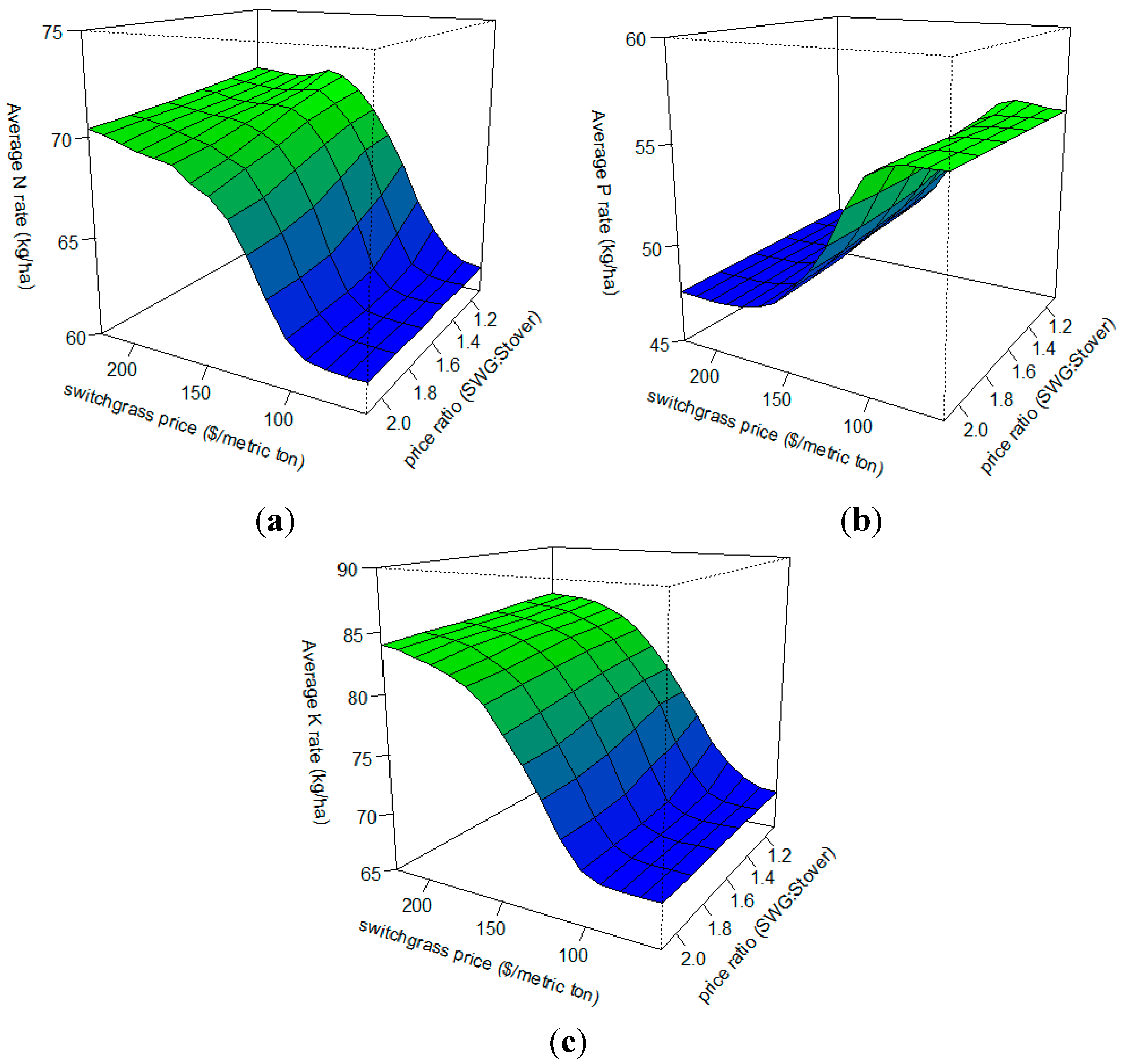
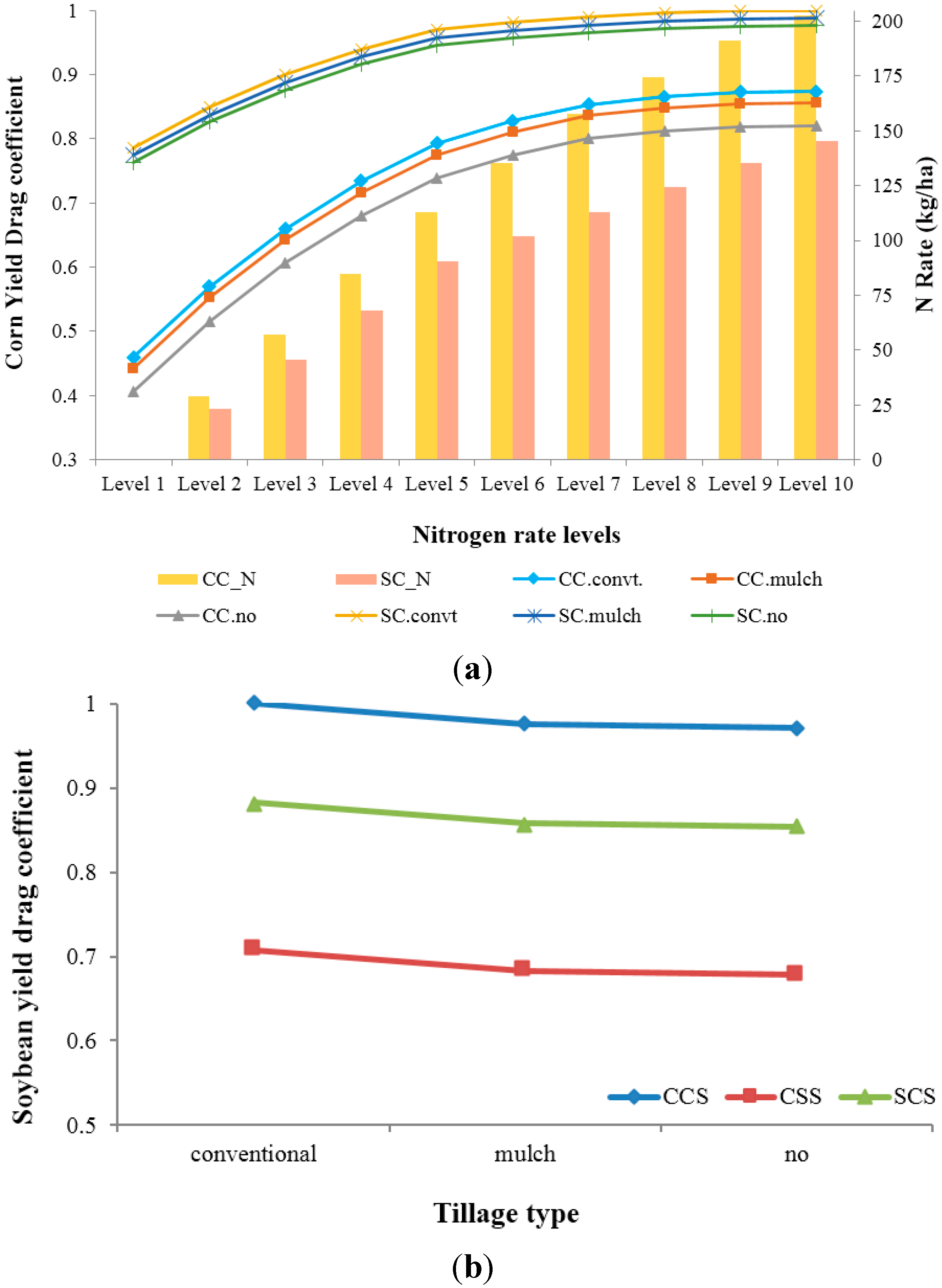
A. Crop Yield Drag Coefficients and Fertilizer Rates

The effects of crop rotation, tillage type, and nitrogen fertilizer rates (corn only) are accounted for when calculating crop yields. Crop yield drag coefficients that capture the rates at which the crop productivity declines as a function of continuous planting, are derived from corn and soybean yield functions [7] and represented in Figure A1. Given the impact of the previous year’s crop, continuous corn (CC) corresponds to lower yield than corn in annual rotation with soybean (SC). Soybean yields in the present year are influenced by the previous two years crops. Among the crop rotation series (corn-corn-soybean: CCS, corn-soybean-soybean: CSS, soybean-corn-soybean: SCS), CCS corresponds to the highest soybean yield, followed by SCS, and then CSS. The impacts of tillage types on crop yields are taken into account for both corn and soybean. Among the three tillage types (conventional tillage, mulch tillage, and no tillage), the crop with conventional tillage has the highest yield and no till has the lowest. Instead of using a quadratic function [7] to characterize corn yield response to nitrogen, ten different levels of nitrogen rates and corresponding corn yield drag coefficients are sampled from the response curve. This implementation reduces the optimization problem from a nonlinear into a linear programming problem.
Figure A1. Corn yield drag coefficients (a) for different rotation, tillage, and N fertilizer rate levels, and soybean yield drag coefficients; (b) for different rotation types: Corn is denoted as “C” and soybean as “S”, the last letter in a rotation pattern means the current crop (e.g., CCS means corn-corn-soybean, and soybean is in the current year).
Land 04 01110 g009
In the model, it is assumed that soybean does not need nitrogen fertilizer. The fertilizer rates of phosphorus (P) and potassium (K) are fixed for soybean: Respectively, 44.83 kg/ha and 84.07 kg/ha. According to Iowa State University Extension [38,51], corn after corn requires lower fertilizer input of phosphorus (P) and potassium (K) than corn after soybean. For corn after corn, the P rate is 61.65 kg/ha and the K rate is 50.44 kg/ha; for corn after soybean, the rates are 67.25 kg/ha and 56.04 kg/ha.
Switchgrass is a perennial with an establishment period. Therefore, we assume that the switchgrass starts to be harvested from the second year. Switchgrass yields depend on soil type. We scale the tall introduced grasses yield (TIGRSYLD) in the Iowa Soil Properties and Interpretations Database (ISPAID) into the data range from 4.48 to 14.35 metric ton/ha to represent the switchgrass yield for different soil types. According to Duffy (2008) [40], in the first year when switchgrass is established nitrogen fertilizer is not required, but 33.63 kg/ha of P and 44.83 kg/ha of K are applied. 112.09 kg/ha of N is applied from the second year on to compensate for the harvest of switchgrass. The amount of P and K applied depends on the amount of switchgrass biomass harvested. For each ton of switchgrass that is harvested, 0.88 kg of P and 10.34 kg of K are applied.
Corn stover yield is estimated as the product of the portion of corn stover harvested and corn yield (we assume that dry weight of corn grain is equal to corn stalk weight). Additional amounts of N, P, and K fertilizers are applied to compensate for the nutrients removed from the soil system by corn stover harvest. 9.07 kg of N, 2.68 kg of P, and 11.34 kg of K are applied per ton of dry matter stover harvest [41].

B. Empirical Parameters and Parameterization

To generate samples from the agricultural landowners and operators survey database for the eight parameters above, we performed the following analysis on the survey responses. Firstly, we considered the respondents who self-identified as farmers. Concerning the parameter Type, the farmer respondents were classified into the four types based on whether they responded to Question 48 and/or 56 (Table A1). Secondly, we performed one-way ANOVA test on the farm sizes (Area) of the four types of farmers. The results showed that there is sufficient evidence (significance level: 0.001) to reject the hypothesis that the farm size means are all equal among the four farmer types. Thirdly, we analyzed the correlation among the other parameters (Table A2). The results do not support the conclusion that Percent1 SWG and Profit SWG are correlated for Type 2 and 3 farmers. Neither is there evidence to suggest that Percent1 Stvr and Profit Stvr are correlated for Type 1 and 3 farmers. But for both Type 2 and 3 farmers, Percent1 SWG and Percent2 SWG are significantly correlated. Similarly, Percent1 Stvr and Percent2 Stvr are significantly correlated for Type 1 and 3 farmers. For Type 3 farmers, Profit SWG and Profit Stvr are significantly correlated as are Percent1 SWG and Percent1 Stvr.
Table A1. Land use survey questions adopted for model parameterization.
Question #Question
3Do you consider yourself a farmer?
18cNumber of acres you own that you farmed in 2009
18dNumber of acres you leased or rented to other people to farm in 2009
18eNumber of acres you rented from others to farm in 2009
18fNumber of acres in the Conservation Reserve Program (CRP) in 2009
48What is the minimum net profit per acre you would need to get in order to consider marketing corn stover?
49If you could get that profit per acre, how many acres of corn stover would you consider harvesting?
50If you supplied corn stover to a bio-refinery, would you prefer to harvest 30%, 50%, or 70% of the corn stover in your fields?
51If you could get a net profit 50% higher than what you indicated in question 48, how many acres of corn stover in total would you consider harvesting?
56What is the minimum net profit per acre you would need to get in order to consider growing switchgrass?
57If you could get that profit per acre, how many acres of switchgrass you consider planting?
58If you could get a net profit 50% higher than what you indicated in question 55, how many acres of switchgrass in total would you consider growing?
Based on the results of this analysis, we used the following strategy to empirically draw 30 samples using the bootstrap sampling method. First, farmer respondents and farmer agents are respectively classified into five groups based on the land acreages they reported (≤40.47, 40.47–121.41, 121.41–202.34, 202.34–303.51, and >303.51 ha). Second, for all agents in a certain group, the sample of parameter Type is drawn from the empirical distribution of Type for farmers in the corresponding group. Third, the remaining parameter values are generated for farmer agents in each group and of each type. For Type 1 agents, parameter values of Profit Stvr, Percent1 Stvr and Portion Stvr are independently generated; parameter values of Percent2 Stvr are associated with Percent1 Stvr. For Type 2 agents, parameter values of Profit SWG, Percent1 SWG are independently generated; parameter values of Percent2 SWG are associated with Percent1 SWG. For Type 3 agents, parameter values for Profit Stvr, Percent1 Stvr, and Portion Stvr are independently generated; parameter values of Profit SWG are associated with Profit Stvr; Percent2 Stvr, Percent1 SWG and Percent2 SWG are associated with Percent1 Stvr.
Table A2. Pearson’s r (p-value) between the parameters characterizing farmers’ attitudes.
TypeProfit SWGPercent1 SWGPercent2 SWGProfit StvrPercent1 StvrPercent2 StvrPortion Stvr
Profit SWG1 or 210.4145 (0.1407)na *nananana
31−0.2488 (0.1560)na0.8471 (2.03 × 10⁻¹¹)nanana
Percent1 SWG1 or 2 10.9687 (4.18 × 10⁻¹¹)nananana
3 10.8885 (1.06 × 10⁻¹²)na0.6822 (3.31×10⁻⁶)nana
Percent2 SWG1 or 2 1nananana
3 1nananana
Profit Stvr1 or 2 10.1918 (0.4768)na−0.0525 (0.8526)
3 1−0.1714 (0.3248)na−0.0648 (0.7033)
Percent1 Stvr1 or 2 10.8897 (9.01 × 10⁻⁶)na
3 10.8952 (1.76 × 10⁻¹³)na
Percent2 Stvr1 or 2 1na
3 1na
Portion Stvr1 or 2 1
3 1
* No Data.

References

  1. O’Neal, M.R.; Nearing, M.A.; Vining, R.C.; Southworth, J.; Pfeifer, R.A. Climate change impacts on soil erosion in Midwest United States with changes in crop management. Catena 2005, 61, 165–184. [Google Scholar] [CrossRef]
  2. Lettenmaier, D.P.; Hooper, E.R.; Wagoner, C.; Faris, K.B. Trends in stream quality in the continental United States, 1978–1987. Water Resour. Res. 1991, 27, 327–339. [Google Scholar] [CrossRef]
  3. Yadav, V.; Malanson, G.P.; Bekele, E.; Lant, C. Modeling watershed-scale sequestration of soil organic carbon for carbon credit programs. Appl. Geogr. 2009, 29, 488–500. [Google Scholar] [CrossRef]
  4. Bekele, E.G.; Lant, C.L.; Soman, S.; Misgna, G. The evolution and empirical estimation of ecological-economic production possibilities frontiers. Ecol. Econ. 2013, 90, 1–9. [Google Scholar] [CrossRef]
  5. Secchi, S.; Gassman, P.W.; Jha, M.; Kurkalova, L.; Kling, C.L. Potential water quality changes due to corn expansion in the Upper Mississippi River Basin. Ecol. Appl. 2011, 21, 1068–1084. [Google Scholar] [CrossRef] [PubMed]
  6. Secchi, S.; Kurkalova, L.; Gassman, P.W.; Hart, C. Land use change in a biofuels hotspot: The case of Iowa, USA. Biomass Bioenergy 2011, 35, 2391–2400. [Google Scholar] [CrossRef]
  7. Kurkalova, L.A.; Secchi, S.; Gassman, P.W. Corn stover harvesting: Potential supply and water quality implications. In Handbook of Bioenergy Economics and Policy; Khanna, M., Scheffran, J., Zilberman, D., Eds.; Springer-Verlag: New York, NY, USA, 2010; pp. 307–323. [Google Scholar]
  8. Lee, K.H.; Isenhart, T.M.; Schultz, R.C.; Mickelson, S.K. Nutrient and sediment removal by switchgrass and cool-season grass filter strips in central Iowa, USA. Agrofor. Syst. 1998, 44, 121–132. [Google Scholar] [CrossRef]
  9. Sarkar, S.; Miller, S.A.; Frederick, J.R.; Chamberlain, J.F. Modeling nitrogen loss from switchgrass agricultural systems. Biomass Bioenergy 2011, 35, 4381–4389. [Google Scholar] [CrossRef]
  10. Parker, D.C.; Manson, S.M.; Janssen, M.A.; Hoffmann, M.J.; Deadman, P. Multi-agent systems for the simulation of land-use and land-cover change: A review. Ann. Assoc. Am. Geogr. 2003, 93, 314–337. [Google Scholar] [CrossRef]
  11. Bennett, D.A.; Tang, W.; Wang, S. Toward an understanding of provenance in complex land use dynamics. J. Land Use Sci. 2011, 6, 211–230. [Google Scholar] [CrossRef]
  12. Matthews, R.; Gilbert, N.G.; Roach, A.; Polhill, J.; Gotts, N.M. Agent-based land-use models: A review of applications. Landsc. Ecol. 2007, 22, 1447–1459. [Google Scholar] [CrossRef] [Green Version]
  13. Robinson, D.T.; Brown, D.G.; Parker, D.C.; Schreinemachers, P.; Janssen, M.A.; Huigen, M.G.A.; Wittmer, H.; Gotts, N.M.; Promburom, P.; Irwin, E.G.; et al. Comparison of empirical methods for building agent-based models in land use science. J. Land Use Sci. 2007, 2, 31–55. [Google Scholar] [CrossRef]
  14. Smajgl, A.; Brown, D.G.; Valbuena, D.; Huigen, M.G.A. Empirical characterisation of agent behaviours in socio-ecological systems. Environ. Model. Softw. 2011, 26, 837–844. [Google Scholar] [CrossRef]
  15. Manson, S.M. Challenges in evaluating models of geographic complexity. Environ. Plan. B Plan. Design 2007, 34, 245–260. [Google Scholar] [CrossRef]
  16. Matthews, R. The people and landscape model (palm): Towards full integration of human decision-making and biophysical simulation models. Ecol. Model. 2006, 194, 329–343. [Google Scholar] [CrossRef]
  17. Matthews, R.; Selman, P. Landscape as a focus for integrating human and environmental processes. J. Agric. Econ. 2006, 57, 199–212. [Google Scholar] [CrossRef]
  18. Epstein, J.M. Generative Social Science: Studies in Agent-Based Computational Modeling; Princeton University Press: Princeton, NJ, USA, 2006. [Google Scholar]
  19. Lansing, J.S.; Kremer, J.N. Emergent properties of Balinese water temple networks: Coadaptation on a rugged fitness landscape. Am. Anthropol. 1993, 95, 97–114. [Google Scholar] [CrossRef]
  20. Le, Q.B.; Park, S.J.; Vlek, P.L.G. Land Use Dynamic Simulator (LUDAS): A multi-agent system model for simulating spatio-temporal dynamics of coupled human-landscape system 2. Scenario-based application for impact assessment of land-use policies. Ecol. Inform. 2010, 5, 203–221. [Google Scholar] [CrossRef]
  21. Le, Q.B.; Park, S.J.; Vlek, P.L.G.; Cremers, A.B. Land-Use Dynamic Simulator (LUDAS): A multi-agent system model for simulating spatio-temporal dynamics of coupled human-landscape system. I. Structure and theoretical specification. Ecol. Inform. 2008, 3, 135–153. [Google Scholar] [CrossRef]
  22. Bousquet, F.; Le Page, C. Multi-agent simulations and ecosystem management: A review. Ecol. Model. 2004, 176, 313–332. [Google Scholar] [CrossRef]
  23. Sengupta, R.; Lant, C.; Kraft, S.; Beaulieu, J.; Peterson, W.; Loftus, T. Modeling enrollment in the Conservation Reserve Program by using agents within spatial decision support systems: An example from southern Illinois. Environ. Plan. B Plan. Des. 2005, 32, 821–834. [Google Scholar] [CrossRef]
  24. Scheffran, J.; BenDor, T. Bioenergy and land use: A spatial-agent dynamic model of energy crop production in Illinois. Int. J. Environ. Pollut. 2009, 39, 4–27. [Google Scholar] [CrossRef]
  25. Ng, T. Response of Farmers’ Decisions and Stream Water Quality to Price Incentives for Nitrogen Reduction, Carbon Abatement, and Miscanthus Cultivation: Preditions Based on Agent-Based Modeling Coupled with Water Quality Modeling. Ph.D. Dissertation, University of Illinois at Urbana-Champaign, Urbana-Champaign, IL, USA, 2010. [Google Scholar]
  26. Ng, T.; Eheart, J.W.; Cai, X.M.; Braden, J.B. An agent-based model of farmer decision-making and water quality impacts at the watershed scale under markets for carbon allowances and a second-generation biofuel crop. Water Resour. Res. 2011, 47. [Google Scholar] [CrossRef]
  27. Schreinemachers, P.; Berger, T. Land use decisions in developing countries and their representation in multi-agent systems. J. Land Use Sci. 2006, 1, 29–44. [Google Scholar] [CrossRef]
  28. Berger, T.; Schreinemachers, P. Creating agents and landscapes for multiagent systems from random samples. Ecol. Soc. 2006, 11, 19. [Google Scholar]
  29. Castella, J.C.; Verburg, P.H. Combination of process-oriented and pattern-oriented models of land-use change in a mountain area of Vietnam. Ecol. Model. 2007, 202, 410–420. [Google Scholar] [CrossRef]
  30. Torii, D.; Bousquet, F.; Ishida, T.; Trébuil, G.; Vejpas, C. Using Classification Learning in Companion Modeling Multi-Agent Systems for Society; Lukose, D., Shi, Z., Eds.; Springer: Berlin/Heidelberg, Germany, 2009; Volume 4078, pp. 255–269. [Google Scholar]
  31. Brown, D.G.; Robinson, D.T. Effects of heterogeneity in residential preferences on an agent-based model of urban sprawl. Ecol. Soc. 2006, 11, 46. [Google Scholar]
  32. Huigen, M.G.A. First principles of the mameluke multi-actor modelling framework for land use change, illustrated with a Philippine case study. J. Environ. Manag. 2004, 72, 5–21. [Google Scholar] [CrossRef] [PubMed]
  33. Castillo, D.; Saysel, A.K. Simulation of common pool resource field experiments: A behavioral model of collective action. Ecol. Econ. 2005, 55, 420–436. [Google Scholar] [CrossRef]
  34. Irwin, E.G.; Bockstael, N.E. Interacting agents, spatial externalities and the evolution of residential land use patterns. J. Econ. Geogr. 2002, 2, 31–54. [Google Scholar] [CrossRef]
  35. Brown, D.G.; Robinson, D.T.; An, L.; Nassauer, J.I.; Zellner, M.; Rand, W.; Riolo, R.; Page, S.E.; Low, B.; Wang, Z.F. Exurbia from the bottom-up: Confronting empirical challenges to characterizing a complex system. Geoforum 2008, 39, 805–818. [Google Scholar] [CrossRef]
  36. Druschke, C.G.; Secchi, S. The impact of gender on agricultural conservation knowledge and attitudes in an Iowa watershed. J. Soil Water Conserv. 2014, 69, 12. [Google Scholar] [CrossRef]
  37. Varble, S.; Druschke, C.G.; Secchi, S. An examination of growing trends in land tenure and conservation practice adoption: Results from a farmer survey in Iowa. Environ. Manag. 2015. [Google Scholar] [CrossRef] [PubMed]
  38. Iowa State University Extension. Nitrogen Fertilizer Recommendations for Corn in Iowa; Leopold Center: Ames, IA, USA, 1997; Available online: http://www.iasoybeans.com/advancenewsletter/PDF/ADV15_0611_4_PM1714.pdf (accessed on 1 October 2015).
  39. Grimm, V.; Berger, U.; DeAngelis, D.L.; Polhill, J.G.; Giske, J.; Railsback, S.F. The ODD protocol: A review and first update. Ecol. Model. 2010, 221, 2760–2768. [Google Scholar] [CrossRef]
  40. Duffy, M. Estimated Costs for Production, Storage and Transportation of Switchgrass; Iowa State University Extension: Ames, IA, USA, 2008; Available online: https://www.extension.iastate.edu/agdm/crops/pdf/a1-22.pdf (accessed on 1 October 2015).
  41. Edwards, W. Estimating a Value for Corn Stover; Iowa State University Extension: Ames, IA, USA, 2014; Available online: https://www.extension.iastate.edu/agdm/crops/pdf/a1-70.pdf (accessed on 1 October 2015).
  42. Johanns, A.M. Iowa Cash Corn and Soybean Prices; Iowa State University Extension and Outreach: Ames, IA, USA, 2015; Available online: http://www.extension.iastate.edu/agdm/crops/pdf/a2-11.pdf (accessed on 1 October 2015).
  43. Food and Agricultural Policy Research Institute. U.S. Baseline Briefing Book: Projections for Agricultural and Biofuel Markets; University of Missouri: Columbia, MO, USA, 2015; Available online: http://www.fapri.missouri.edu/wp-content/uploads/2015/03/FAPRI-MU-Report-01-15.pdf (accessed on 1 October 2015).
  44. Food and Agricultural Policy Research Institute. Competition for Biomass among Renewable Energy Policies: Liquid Fuels Mandate versus Renewable Electricity Mandate; University of Missouri: Columbia, MO, USA, 2011; Available online: http://www.fapri.missouri.edu/wp-content/uploads/2015/02/FAPRI-MU-Report-11-11.pdf (accessed on 1 October 2015).
  45. Davidson, D. Corn on Corn: How Much Yield is Enough; Progressive Farmer: Birmingham, AL, USA, 2007. [Google Scholar]
  46. Smith, P. The Pros and Cons of Going corn-on-Corn; Fields of Facts: Brandon, MS, USA, 2013; Available online: http://agfax.com/2013/09/23/the-pros-and-cons-of-going-corn-on-corn/ (accessed on 1 October 2015).
  47. Edwards, W.; Johanns, A.M. Cash Rental Rates for Iowa 2012 Survey; Iowa State University Extension and Outreach: Ames, IA, USA, 2013; Available online: https://www.extension.iastate.edu/agdm/wholefarm/pdf/c2–10_2012.pdf (accessed on 1 October 2015).
  48. McLaughlin, S.B.; Walsh, M.E. Evaluating environmental consequences of producing herbaceous crops for bioenergy. Biomass Bioenergy 1998, 14, 317–324. [Google Scholar] [CrossRef]
  49. Lee, K.H.; Isenhart, T.M.; Schultz, R.C. Sediment and nutrient removal in an established multi-species riparian buffer. J. Soil Water Conserv. 2003, 58, 1–8. [Google Scholar]
  50. Mann, L.; Tolbert, V.; Cushman, J. Potential environmental effects of corn (Zea mays L.) stover removal with emphasis on soil organic matter and erosion. Agric. Ecosyst. Environ. 2002, 89, 149–166. [Google Scholar] [CrossRef]
  51. Iowa State University Extension. A General Guide for Crop Nutrient and Limestone Recommendations in Iowa; Iowa State University Extension and Outreach: Ames, IA, USA, 2013; Available online: http://store.extension.iastate.edu/Product/A-General-Guide-for-Crop-Nutrient-and-Limestone-Recommendations-in-Iowa-PDF (accessed on 1 October 2015).

