Article

Globalland30 Mapping Capacity of Land Surface Water in Thessaly, Greece

by
Ioannis Manakos
1,*,
Konstantinos Chatzopoulos-Vouzoglanis
1,
Zisis I. Petrou
1,
Lachezar Filchev
2 and
Antonis Apostolakis
3
1
Information Technologies Institute, Centre for Research and Technology Hellas (CERTH–ITI), 6th km Xarilaou—Thermi, 57001 Thessaloniki, Greece
2
Remote Sensing and GIS Department, Space Research and Technology Institute, Bulgarian Academy of Sciences (SRTI–BAS), Acad. G. Bonchev St., block.1, 1113 Sofia, Bulgaria
3
Greek Biotope/Wetlands Centre, The Goulandris Natural History Museum, 14th km Thessaloniki—Mihaniona, 57001 Thermi, Greece
*
Author to whom correspondence should be addressed.
Land 2015, 4(1), 1-18; https://doi.org/10.3390/land4010001
Submission received: 13 November 2014 / Accepted: 17 December 2014 / Published: 23 December 2014

Abstract

:
The National Geomatics Center of China (NGCC) produced Global Land Cover (GlobalLand30) maps with 30 m spatial resolution for the years 2000 and 2009–2010, responding to the need for harmonized, accurate, and high-resolution global land cover data. This study aims to assess the mapping accuracy of the land surface water layer of GlobalLand30 for 2009–2010. A representative Mediterranean region, situated in Greece, is considered as the case study area, with 2009 as the reference year. The assessment is realized through an object-based comparison of the GlobalLand30 water layer with the ground truth and visually interpreted data from the Hellenic Cadastre fine spatial resolution (0.5 m) orthophoto map layer. GlobCover 2009, GlobCorine 2009, and GLCNMO 2008 corresponding thematic layers are utilized to show and quantify the progress brought along with the increment of the spatial resolution, from 500 m to 300 m and finally to 30 m with the newly produced GlobalLand30 maps. GlobalLand30 detected land surface water areas show a 91.9% overlap with the reference data, while the coarser resolution products are restricted to lower accuracies. Validation is extended to the drainage network elements, i.e., rivers and streams, where GlobalLand30 outperforms the other global map products, as well.

Graphical Abstract

1. Introduction

Globally, coordinated governance strategies and international supportive tools and mechanisms (such as the Global Earth Observation System of Systems Water Cycle Integrator—GEOSS-WCI [1]) have been developed to monitor the water reserves under contemporary complex multi-stressor conditions. The high importance and significance of the water resources, their monitoring and their sustainable management through geoinformation technologies have been outlined in the Water Framework (Directive 2000/60/EC), Flood risk (Directive 2007/60/EC), and INSPIRE (Directive 2007/2/EC) Directives. Earth Observation (EO) and Remote Sensing (RS) in particular, are gradually gaining momentum for water resource monitoring, whereas recently deployed and upcoming European remote sensing missions (i.e., the Sentinel series) are expected to improve current acquisition capabilities, both in terms of resolution and reliability [2]. This is clearly visible at the international reports prepared for the status of world water resources by the United Nations Economic Commission in Europe (UNECE) and World Meteorological Organization (WMO), to name but a few [3,4].
Furthermore, the importance of water monitoring is highlighted by the inclusion of an inland water layer among the five High Resolution Layers (HRL) of 20 m spatial resolution (the other four layers being “imperviousness”, “forests”, “permanent grasslands” and “wetlands”) meant to be produced and updated every three years according to the Copernicus land service objectives [5]. Certain layers of Land Cover Component description are employed in the recently proposed EAGLE model (European Topic Centre on Spatial Information and Analysis—Action Group on Land monitoring in Europe) to characterize water elements in detail [6], further highlighting the significance of water monitoring.

1.1. Background

The extraction of a global land cover map has been firstly attempted using 8 km spatial resolution National Oceanic and Atmospheric Administration (NOAA) Advanced Very High Resolution Radiometer (AVHRR) data [7,8]. The AVHRR data of 1 km spatial resolution were later used for the production of a global LU/LC map from the University of Maryland [9] and the International Geosphere-Biosphere Programme (IGBP) DISCover global map [10,11]. The one-kilometer AVHRR data were further employed in the production of a land cover map at a pan-European scale [12,13]. The AVHRR started being replaced by sensors with better spatial or spectral characteristics. Friedl et al. [14] initially produced a 1 km spatial resolution map using Moderate Resolution Imaging Spectroradiometer (MODIS) data; 500 m spatial resolution data were employed later, leading to a higher resolution map [15]. Furthermore, MODIS data were used for the production of the Global Land Cover by National Mapping Organizations (GLCNMO) map for 2003 and a second version for 2008, with 1 km and 500 m spatial resolution, respectively, under the Global Mapping project [16,17]. An international partnership coordinated by the European Commission’s (EC) Joint Research Centre (JRC) employed data from the SPOT VEGETATION sensor to produce a global land cover of 2000 (GLC2000) map with spatial resolution equal to 1 km at the equator [18]. The spatial resolution of the produced maps was further increased with the use of Medium Resolution Imaging Spectrometer (MERIS) data in the GlobCover map products to 300 m for 2005/2006 (v2.2) and 2009 (v2.3) [19,20,21,22], as well as in the GlobCorine 2009 product of the same spatial resolution [23,24].

1.2. Most Recent Developments

The extent of the “land surface water” class (LSW), whose accuracy is put under examination in this study, varies over time due to seasonal fluctuations of the precipitation and evapotranspiration regime over an area. The latter are shifting the exact position of the waterline, which delineates the open water surface from the mainland, and influencing the ability to trace it [25]. Single image acquisitions may capture the snapshot in time, and as such, may be considered as proxy for the real situation on the surface. Time series data, comparable to the scale used for the climate definition of an area, are required for the safe designation and, if possible, quantification of this part of the water cycle. Foody et al. [25] reported root mean-square error (RMSE) values of 2.25 m for waterlines extracted from SPOT HRV satellite data with 20 m spatial resolution, which satisfied the accuracy requirements for a large-scale 1:5000 LU/LC mapping. Still, the very high spatial resolution aerial photography achieved less error estimates, i.e., below 5%, when mapping LSW [26]. Landsat TM and ETM+ data have also been employed for the mapping of water bodies in different studies, with classification accuracies varying between 80% and 95%, depending on the method used [27,28,29].
With the advancement of remote sensing technologies and data availability, moderate to high spatial resolution remotely sensed images have been increasingly used to monitor and map water bodies different in size and shape, including the land surface water bodies (LSW) [30,31,32,33]. Products of global coverage were envisaged under the National Aeronautics and Space Administration (NASA) and the United States Geological Survey (USGS) Global Land-Cover Data Initiative, mainly employing Landsat data [34]. In Europe, the GIO (Global Monitoring for Environment and Security (GMES) Initial Operations) Pan-European layers with 20 m spatial accuracy are expected in full extent in the upcoming period [35]. In Asia, global maps of unprecedented resolution of 30 m have been produced by China’s 30-metre Global Land Cover mapping project (GlobalLand30) for 2000 and 2009/2010 [36,37].
More specifically, the GlobalLand30 has been the outcome of the effort of the Chinese Ministry of Science and Technology to create a global land cover product of higher spatial resolution for the years 2000 and 2009/2010 [36,37,38]. The goal of this endeavor was to meet with the needs of global environmental change studies and earth systems simulation [38]. For this purpose, Landsat data have been primarily used, together with MODIS data and data from the Chinese satellites HJ, Beijing-1 and the Chinese weather satellite. The final product overall spatial resolution is 30 m [39]. Land cover classes are extracted in six sequential stages of the classification approach, namely: (1) “water”; (2) “wetland”; (3) “snow and ice”; (4) “artificial cover”; (5) “cropland”; and (6) “forest, shrubland, grassland and barren land” [40]. The “water” class layer is extracted at the first stage of the approach, using reflectance properties, and categorized as “clear, green or turbid water” [40]. A precise mapping of GlobalLand30 inland open waters for both years 2000 and 2010 was conducted in 2012 [41]. Nowadays the complete global land cover mapping is released following its validation [42].
A main objective of the study is to assess the accuracy of the Chinese LSW class (GlobalLand30-Water) juxtaposed against detailed ground truth data on a representative area in the Mediterranean, the region of Thessaly, Greece. Furthermore, in order to quantitatively demonstrate the capacity upgrade brought along with GlobalLand30-Water, the outcomes are set aside to the respective LU/LC thematic classes from GlobCover 2009 [22], GlobCorine 2009 [23,24], and Japan’s Global Land Cover map [16,17,43]. The particular layers were selected in order to have a three-step scale comparison sequence, i.e., at spatial resolution of 500 m, 300 m, and 30 m, and be able to delineate the current trend.

2. Study Area and Materials
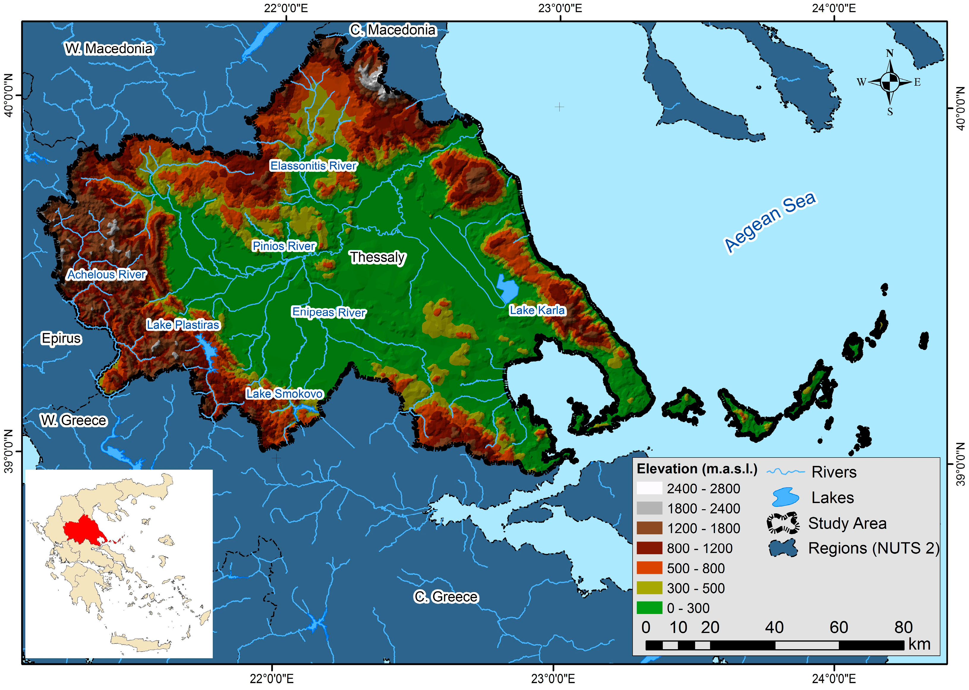
2.1. Study Area

The Thessaly Region is located in the center of Greece (Figure 1) and shares borders with the regions of Central and Western Macedonia, Epirus and Central Greece, while its eastern part is bordering the Aegean Sea. It occupies 10.6% (14,037 km2) of the total surface of the country. The region’s geomorphological landscape consists of mountainous parts on the perimeter and lowlands in the center. More specifically, 37% of the region’s surface is flat, 16.8% is semi-mountainous and 46.2% is mountainous [44]. There are five mountains, including Mount Olympus, with an altitude of 2917 m above sea level (a.s.l.), being the highest in Greece. The average altitude of the region is 285 m a.s.l.
Figure 1. Map of the study area.
Land 04 00001 g001
The Thessaly Region is divided into three areas with a varying precipitation pattern: (1) the eastern coastal and mountainous; (2) the central plains; and (3) the western mountainous. In the whole water district, the average annual rainfall is estimated at 678 mm [45]. The amount of atmospheric precipitation in the water district is larger in the West, then reduced to the plain and rising again in the mountainous Eastern part. The total average annual flow of all rivers of Thessaly region is 3.54 billion m3. The average annual temperature ranges from 16 °C to 17 °C. The annual temperature amplitude exceeds 22 °C. The warmest months are July and August and the coldest January, February, and December. Frost-kills are frequent and occur from November to April [46].

2.2. Materials

The data used in the present study originate from various sources: institutional databases and intermediate products, satellite images, orthophotos, and thematic raster layers. A full list of the available data utilized is provided (Table 1 [47,48,49,50,51,52,53]). In particular, Hellenic Cadastre (HC) orthophotomap was created by color orthophotos through aerial surveys performed between 2007 and 2009. The surveys covered almost the entire area of Greece and were coordinated by the National Cadastre & Mapping Agency S.A. (NCMA S.A.). The non-urban areas, as the one studied, have 0.5 m spatial resolution, while their geometric accuracy (RMSExy) is ≤1.41 m (confidence level 95%). The GlobalLand30-Water considered was generated from Landsat TM/ETM+ 2009 images (spatial resolution of 30 m) for Thessaly, Greece. The Landsat TM/ETM+ images have proven to be capable of accurately classifying a large variety of landscapes including the heterogeneous Mediterranean landscapes [54,55,56].
Table 1. Data sources and data types used in the present study.
Data SourceTypeMinimum Mapping Unit
RapidEye [50]Raster6.5 × 6.5 m2
Inland Water Map (GlobalLand30-Water) [National Geomatics Center of China (NGCC) [51]Raster30 × 30 m2
GlobCover 2009 © ESA 2010 and UCLouvain [52]Raster300 × 300 m2
GlobCorine 2009 © ESA 2010 and UCLouvain [53]Raster300 × 300 m2
Global Land cover map (GLCNMO) version 2, 2008 (Geospatial Information Authority of Japan, Chiba University and collaborating organizations) [54]Raster500 × 500 m2
Hellenic Cadastre (HC) Copyright © 2014, National Cadaster and Mapping Agency S.A., orthophoto map 2007–2009 [55]Raster50 × 50 cm2
Drainage network Greek Ministry of Environment, Energy and Climate Change (GMEECC) [56]VectorScale: 1:50000

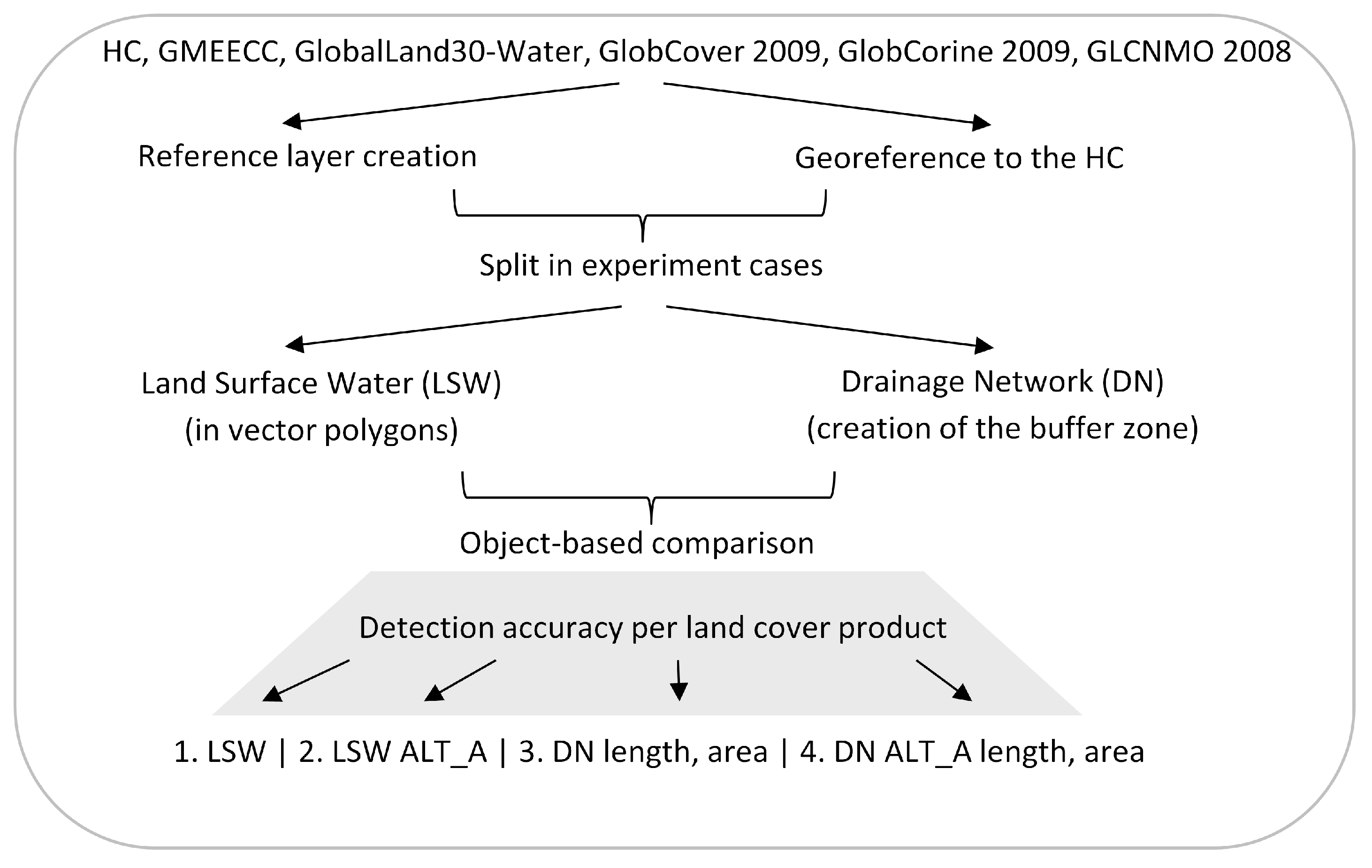
3. Experimental Section

3.1. Class Definitions

According to the Chinese GlobalLand30 product terminology, inland water class is defined as “accumulated liquids of water generated naturally or artificially on the earth’s surface, which is not covered by any vegetation, including river (canal), lake, reservoir, etc.” [40]. As explicitly mentioned, this class is distinguished from sea water, ice, snow, wetlands, and paddy fields.
The GlobCover 2009’s respective class definition is “artificial and natural water bodies,” with class ID/code “210” [57], GlobCorine 2009’s relevant class description is “water bodies” with class ID/code “200”, and GLCNMO 2008’s class definition is: “The land cover consists of artificial water bodies. A further specification can be made in flowing or standing water. The land cover consists of natural water bodies. A further specification can be made in flowing or standing water,” with class ID/code “20” [17].

3.2. Reference Data Set Creation

While using input data from different but relatively close to each other dates, a degree of uncertainty may be introduced into the procedure, since the extent of open water body undergoes fluctuations over time, especially under the Mediterranean climatic conditions. No timely extended record (i.e., for decades) exists for the derivation of the reference data in order to have a precise image of the permanent flooded area in question. Both the reference data and the data to be evaluated are considered as snapshots in time, timely close enough to be compared, as best proxies for the situation on the ground. In this study the following procedure was undertaken:
(a)
The visual interpretation and water areas’ polygons digitization on screen was supported by an initial recognition of possible water covered areas. In favor of their availability, autumn RapidEye images of 2011 have been classified to create an initial polygon layer to capture the land surface water areas. The summer dry period prior to the acquisition enhanced the detectability of water areas’ boundaries that are maintained throughout the year. Pixel based supervised classification was performed in order to identify water and non-water classes. It aimed solely for rapid pre-identification of possible water covered areas. Confirmation or rejection of these polygons was later undertaken based on the Hellenic Cadastre (HC) base map.
(b)
With the additional calculation of the normalized difference vegetation index (NDVI) [58] and the NDWI [59] layers from the RapidEye images, further possible areas indicating increased wetness were derived. Following this procedure, a preliminary list of 816 polygons describing the detectable wetness areas was generated in an effort to capture all water covered areas, to minimize, if not eliminate, the omission error for the extent of the study area.
(c)
In this step photointerpretation took place. In order to counterbalance definition discrepancies, LSWs were considered as the areas, where water covering the underlying ground (water table) could be visible while looking from above (air or satellite operating height). Extensive evaluation of each point was performed, supported by the Hellenic Cadastre (HC) base map. Via the use of the HC, the presence of LSW around the 816 centroids of the previously extracted polygons was searched. Through the HC map, 682 water bodies were finally delineated through visual interpretation and digitized as polygons on screen.
(d)
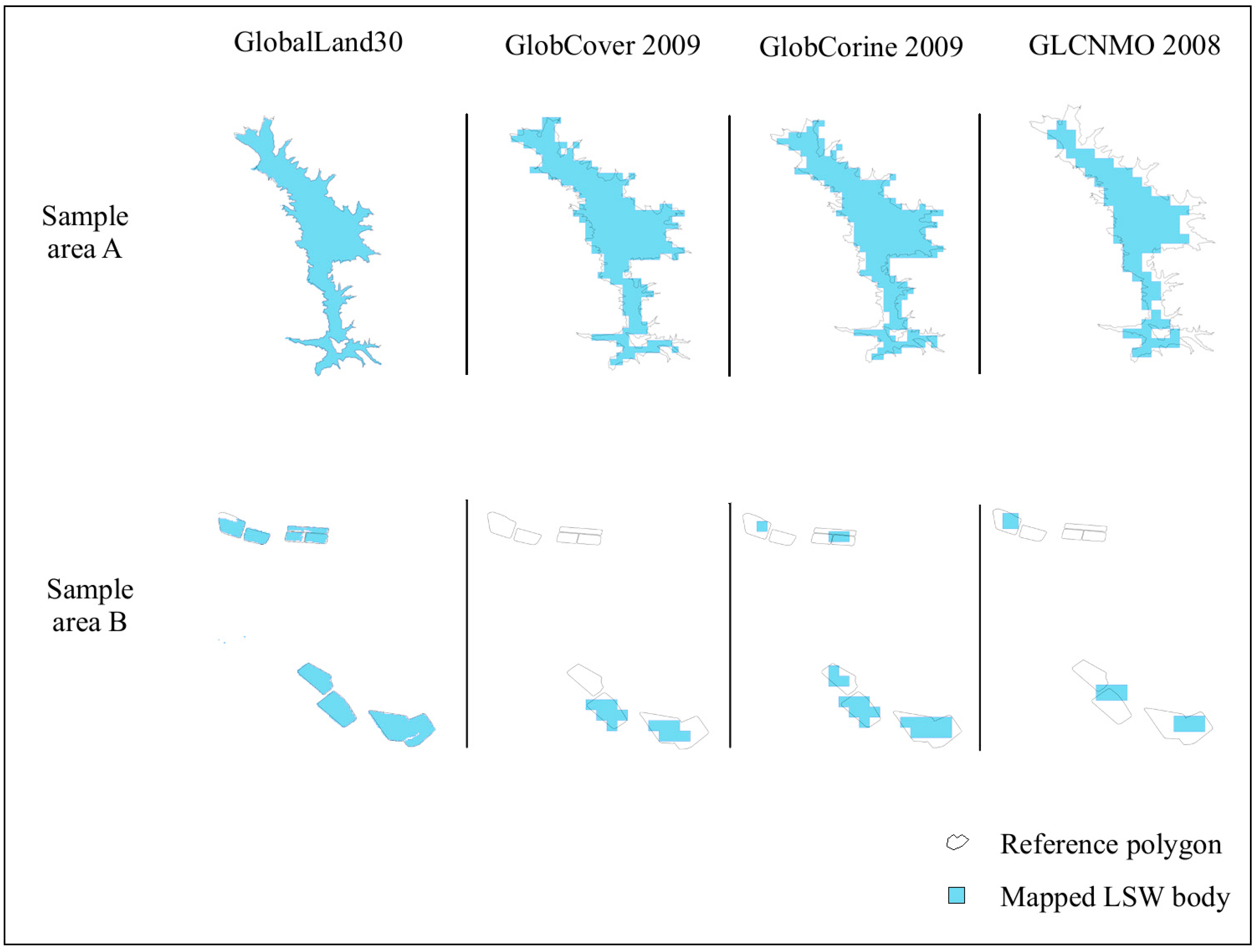
These polygons were overlapped with the time series of very high resolution satellite images derived from Google Earth (GE) software [60]. Parts of the study area were covered by coarse resolution GE images, when the respective acquisition series around the global layers’ production years and seasons were sought (summer 2009, 2009, 2009, 2008) for the 4 layers (GlobalLand30, GlobCover 2009, GlobCorine 2009, and GLCNMO 2008). These partial areas were masked out during the evaluation process and the respective polygons were removed from the reference layer accordingly.
(e)
For the remaining polygons very high resolution (<4 m) GE imagery partial snapshots of the enclosed surface and their imminent surroundings were acquired and co-registered via control points’ coordinates to the HC equivalent sub-areas with RMSExy ≤ 4 m. Selected GE very high resolution imagery parts of the same, previous, and following year are incorporated into the evaluation process to cope with the seasonality fluctuation of the land surface water bodies. Then the initially delineated reference polygons were re-digitized and reshaped according to the open water surface extent of the GE partial imageries using photointerpretation. Knowledge of the local conditions in relation to artificial boundaries of several land surface water areas was incorporated into the procedure. In cases of uncertainty or discrepancy the closest imagery date and/or smaller polygon area was favored to cope for the generally prevailing evapotranspiration conditions of the area.
Following the aforementioned analysis of RapidEye, HC and GE time series imageries for the areas of interest, a final reference polygon layer of 132 polygons was generated, upon which the accuracy assessment took place.

3.3. GlobalLand30-Water Accuracy Assessment Approach

The GlobalLand30-Water was georeferenced in WGS84, the same projection system as the HC polygon and Greek Ministry of Environment, Energy and Climate Change (GMEECC) linear shapefiles. Initially, minor registration errors were detected through visual inspection. In order to resolve this problem, a relative georeferencing was performed. Ten uniformly distributed points were selected and a second order polynomial transformation of the GlobalLand30-Water layer was conducted to better co-align with the HC derived map. The outcome of this procedure achieved an accuracy of RMSE of 8.65 m, which is below the 1/3 of the pixel spatial resolution (30 m) of the GlobalLand30-Water raster maps. Figure 2 demonstrates the registration accuracy between the reference and the GlobalLand30-Water layers for two sample areas. In addition, the respective registration outcomes with the GlobCover 2009, GlobCorine 2009, and GLCNMO 2008 LSW layers, as discussed below, are also depicted.
The GlobalLand30-Water raster map was then transformed into a vector polygon file, following exactly the edges of the raster pixels, in order to be compared with the reference LSW map. The common areas between the GlobalLand30-Water-derived polygons and the LSW digitized ones were isolated using an intersection tool to calculate the overlap percentage, i.e., the ratio of the intersection areas to the total LSW areas multiplied by 100. In addition, an alternative approach (ALT_A) for the comparison of the derived HC reference layer with the GlobalLand30-Water map is followed, excluding all the water bodies from the HC LSWs that are smaller than the spatial resolution of the GlobalLand30-Water map. In particular, for the comparison of HC LSWs with the GlobalLand30-Water, every polygon with an area smaller than 30 m × 30 m, i.e., 900 m2, was excluded in the ALT_A (Figure 3).
Figure 2. Registration performance visualization between the reference and the GlobalLand30, GlobCover 2009, GlobCorine 2009, and GLCNMO 2008 LSW layers, for two representative sample areas.
Land 04 00001 g002
Figure 3. Methodology workflow (ALT_A: Alternative Approach; for HC, GMEECC, GlobalLand30-Water, GlobCover 2009, GlobCorine 2009, GLCNMO 2008 see Table 1).
Land 04 00001 g003
Specifically for the linearly aligned surface features, such as the drainage network (DN), the GMEECC maps were used to identify the locations of the rivers with a constant flow of water. Then, they were digitized in detail as vectors on the HC base map through a similar visual interpretation and on-screen digitization process, as reported previously. This was necessary since the scale of the GMEECC data is coarser than the one necessary for this study. Next, a stream order classification according to Strahler [61] took place, with the higher order rivers being the ones accumulating the whole amount of water at the end of the flow to the sea. The 1st, 2nd, 3rd, and 4th order rivers were then compared with the GlobalLand30-Water map to assess the degree their existence, length, and area were able to be registered on it:
  • Their length was calculated by comparing the length of the rivers extracted by the GlobalLand30-Water with the total length of the digitized rivers.
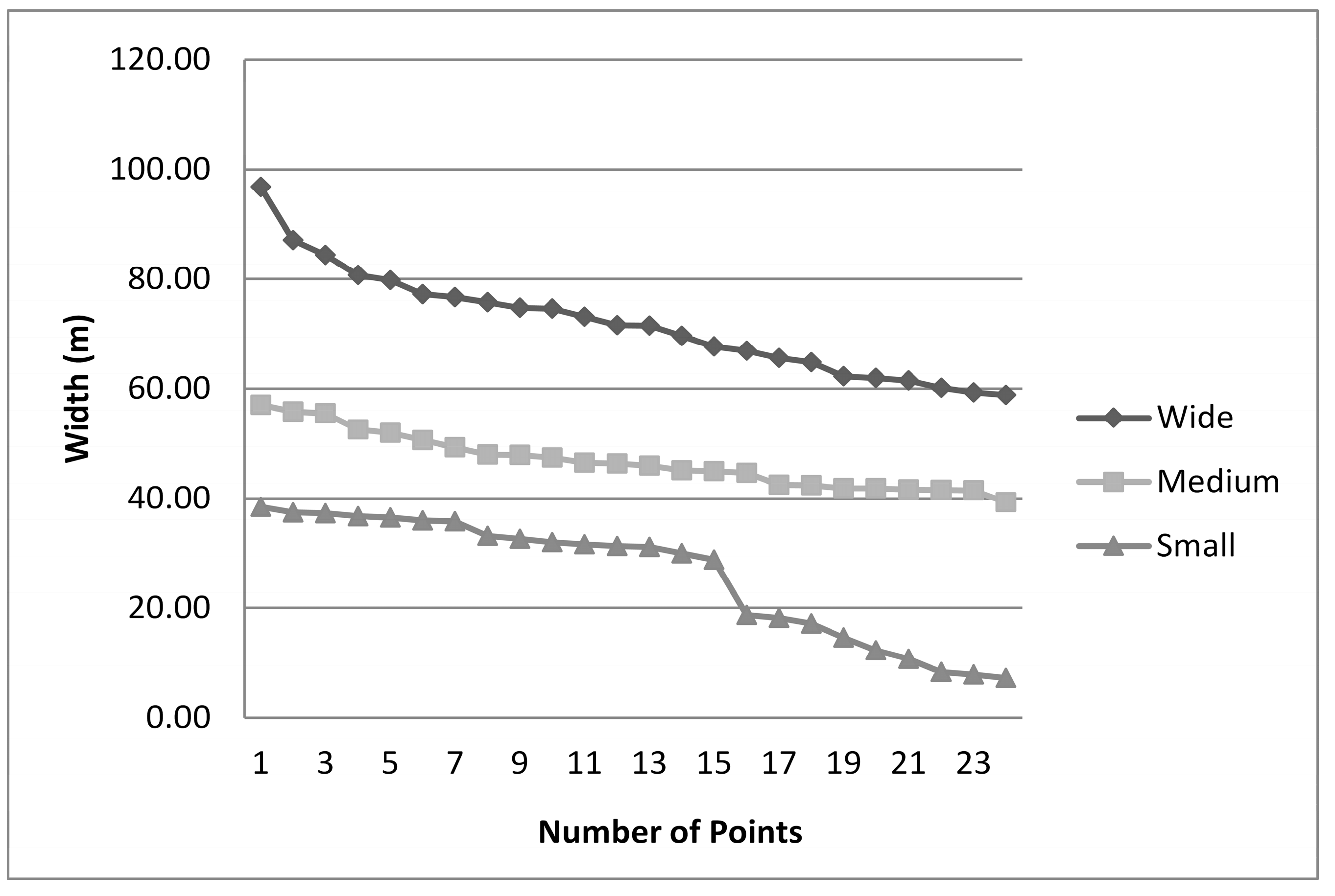
  • In regard to the extent of the open water area present in the rivers, a different method was followed to avoid the time-consuming digitization of this large area. At a representative number of points, randomly distributed on the DN, transects across the rivers were digitized, enabling the measurement of each transect’s width. The widths were ranked in a list from higher to lower, then categorized into 3 groups and each group’s average width was calculated. The rivers were then divided into linear subparts according to their width as estimated from the GE imagery (each subpart had a low variance of individually measured widths), buffered automatically with a radius of the respective average width and re-arranged (digitized again) in 3 different linear shapefiles, namely “Wide”, “Medium”, and “Narrow” (Figure 4). It is worth mentioning that in the “Narrow” class there were points that could belong to a 4th group with significantly smaller width. This group was intentionally left out, because of the average class width of 26 m that was already lower than GlobalLand30-Water spatial resolution. These buffered regions were thereafter overlaid with the GlobalLand30-Water equivalent areas.
Figure 4. The width of the selected river transects across the area subdivided in three groups.
Land 04 00001 g004

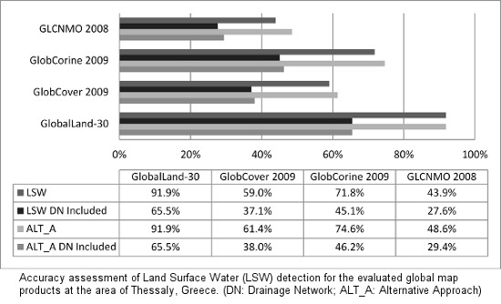
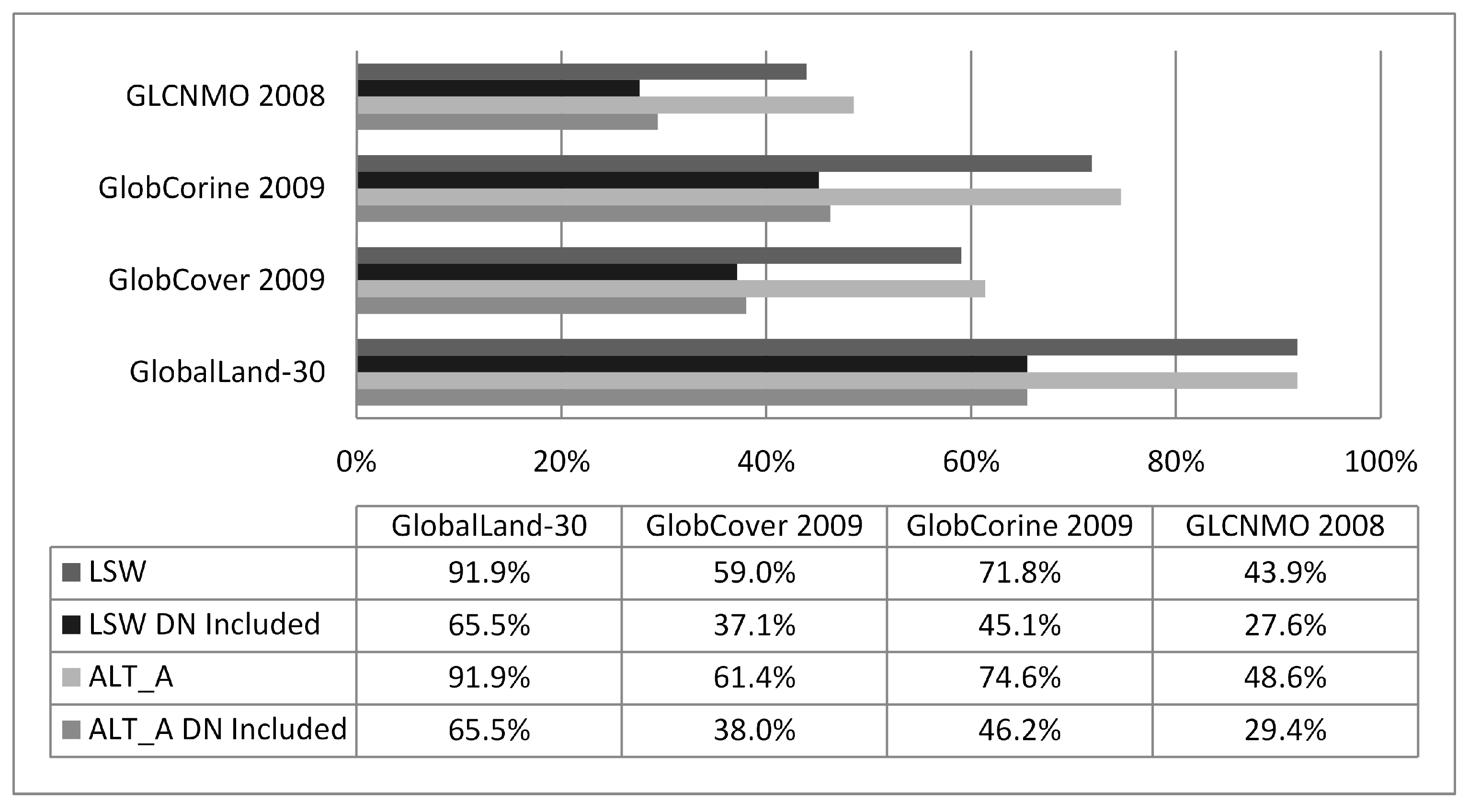
3.4. GlobCover 2009, GlobCorine 2009 and GLCNMO 2008 Accuracy Assessment Approach

Following the procedure described in Section 3.3, the water body classes of GlobCover 2009, GlobCorine2009, and GLCNMO 2008 were isolated and digitized in polygon files and then intersected with the upgraded reference file (Figure 2). Finally, the intersection area was calculated and compared with the HC LSWs area to find the specific percentage of the overlap. Validation was performed following both the main and the ALT_A approaches. The DN was totally excluded, since the maximum river width was ≈100 m and could not be detected by the 300 m spatial resolution of the GlobCover 2009 and GlobCorine2009 maps or the 500 m spatial resolution of the GLCNMO 2008 map.

4. Results

The comparison between the timely upgraded HC LSW and GlobalLand30-Water revealed that there was a 91.9% area overlap, whereas the evaluation assessment with the GlobCover 2009, GlobCorine 2009, and GLCNMO 2008 products showed overlaps in the range of 59%, 71.8%, and 43.9%, respectively. The ALT_A approach increased the performance of the GlobCover 2009, GlobCorine 2009, and GLCNMO 2008 layers to 61.4%, 74.6%, and 48.6%, respectively (Figure 5).
The DN comparison shows that 13 out of 22 rivers and streams were identified (even partially) by the GlobalLand30-Water map (Figure 6), while no rivers could be detected by the GlobCover 2009, GlobCorine 2009, and GLCNMO 2008. In addition, there was 36.8% overlap in terms of length and 22% overlap in terms of area.
Figure 5. Accuracy assessment results (for GlobalLand30-Water, GlobCover 2009, GlobCorine 2009, and GLCNMO 2008: see Table 1). LSW: Land surface water detection with the main approach; LSW DN included: Land surface water and Drainage network detection with the main approach; ALT_A: Land surface water detection with the alternative approach; ALT_A DN included: Land surface water and Drainage network detection with the alternative approach.
Land 04 00001 g005
Figure 6. GlobalLand30-Water identified rivers following the categorization after Strahler [61], represented by the x-axis. The y-axis draws the number of 1st, 2nd, 3rd, and 4th order rivers.
Land 04 00001 g006
The total overlapping percentage of both timely upgraded HC LSW and DN compared with the respective ones of GlobalLand30-Water derived areas is 65.5%. It was calculated by dividing the total GlobalLand30-Water overlap area into the total LSW + DN area. Contrarily, GlobCover 2009, GlobCorine 2009, and GLCNMO 2008 accuracies drop significantly to 37.1%, 45.1% and 27.6%, respectively, if the DN areas are included in the accuracy assessment (Figure 5).

5. Discussion

Assessment and intercomparison of remote sensing mapping products, especially of global scale, has been identified as a challenging process. Usual limitations include inconsistencies amongst accuracy assessments performed individually for each product, unavailability of adequate reference data or inappropriate sampling, and disparities in map spatial resolution or class definitions [62,63,64]. Several efforts have been undertaken to validate the accuracies of the different global land cover products. The validation efforts have been often performed individually for each product, using different approaches and reference data sets, while in a few cases comparative analyses involving some of the products have been performed [65,66,67]. Their reported global accuracies vary from 66.9% (IGBP DISCover), 67.5% (GlobCover 2009), and 68.6% (GLC2000), to over 70%, namely 76.5% (GLCNMO 2003) and 78.3% (MODIS) [16,23,67].
The validation process proposed in this study allows for a quantitative outcome in relation to the accuracy of four of the recent and commonly used global LU/LC products in detecting inland water bodies (e.g., lakes, permanent water bodies) and linear elements (e.g., rivers), as important layers of information in a variety of applications and decision making processes. Although individual assessments of the employed GlobalLand30-Water, GlobCover 2009, GlobCorine 2009, and GLCNMO 2008 products have been presented in different studies [16,22,24,40], validation using a common reference layer has not been previously reported. The present study, thus, allows a straightforward verification of the products on a common ground.
The validation strategy of this study complies with the general notion that the only feasible way to acquire reference points for global mapping validation is by photointerpretation of high resolution data, compared with the lower resolution mapping products [62]. In particular, numerous studies have used Google Earth imagery (e.g., QuickBird, IKONOS) to validate products mainly from MODIS or Landsat, at a local or global scale, including urban areas [68], taiga–tundra transition zones [69], mangrove forests [70], irrigated areas [71], channels and oxbow-lakes [72], or oases in desert regions [73]. In this study, two further layers of very high resolution images, namely RapidEye imagery and airborne cadastral orthophotos, have been employed besides Google Earth imagery to create a high precision validation layer.
As shown in Figure 5, the GlobalLand30-Water map identified LSWs with an accuracy of 91.9%. The achieved accuracy falls within the required error rates of 5%–15% reported by users as the maximum tolerable to be used in further modeling applications [74]. The respective accuracy for the GlobCover 2009 product reaches 59%, and for the GlobCorine 2009 product 71.8%, while for GLCNMO 2008 up to 43.9%. This is a clear indication that the spatial resolution of the primary data used for land cover applications plays a significant role: moving from the coarse spatial resolution of 500 m to finer spatial resolution, the achieved accuracies seem to be improving, being doubled or more in resolutions of 30 m.
Similar outcome may be derived by comparing the achieved accuracies for the detection of linear water elements, such as rivers. In this case the absolute accuracy of the GlobalLand30-Water product has decreased to 65.5%. However, its relative advantage over GlobCover 2009, GlobCorine 2009, and GLCNMO 2008 has further increased, compared with the reference LSW elements (Figure 5). In general, linear elements seem to be significantly harder to detect by any product, due to their width.
The exclusion of landscape elements smaller than the map spatial resolution, under the ALT_A approach, slightly improved the detection results for all maps, with the coarse spatial resolution ones being more favored than the GlobalLand30-Water product, where a very slight improvement of less than 0.1% is observed, suggesting the efficiency of the product in detecting water bodies under real-life conditions. Nevertheless, under the ALT_A approach, the GlobalLand30-Water outperforms the GlobCover 2009 and the GlobCorine 2009 products by 19.2%–27.5% (in terms of thematic accuracy) and the GLCNMO 2008 product by 36.1%. In case only the LSW’s accuracies are compared, the picture is even sharper, which means that low to medium spatial resolution global land cover products, such as GlobCover 2009, GlobCorine 2009, and GLCNMO 2008 are not adequate to map the inland open water bodies in Mediterranean environments.

6. Conclusions

This study contributes to the global assessment of the improvement achieved by the production of global land cover layers; it demonstrates the applicability of GlobalLand30-Water product to surface water resources management in the region of Thessaly, an indicative region of the Northern Mediterranean, as a tool accurately detecting inland water. It covered a gap of validation about the performance of the newly released GlobalLand30 in Mediterranean conditions. Apart from the quantitative analysis of the adaptability of the GlobalLand30-Water map to the real conditions in the study area, it discussed and quantitatively demonstrated the trend that global land cover mapping follows nowadays, improving the spatial resolution from 500 m to 30 m.
The performance of four global land cover products was assessed, i.e., GlobalLand30-Water, GlobCover 2009 (class: 210), GlobCorine 2009 (class: 200), and GLCNMO 2008 (class: 20), to identify the LSW thematic class in the study area. The study utilized an object-based comparison approach to detect accuracies per land cover product. Reference layers were based on HC orthophoto maps and RapidEye and Google Earth image data.
It was found out that 91.9% of the classified area by GlobalLand30-Water successfully coincides with the reference data layer. In comparison, the GlobCover 2009 achieved 59%, the GlobCorine 2009 reached higher, up to 71.8%, whereas the GLCNMO 2008 performed lower than both, with 43.9% accuracy. The result allows concluding that a global land cover product with 30 m spatial resolution is accurate enough for the thematic assessment of land surface water bodies in the Mediterranean. In addition, for linear drainage surface water features, the use of an ancillary knowledge base about the area under investigation or higher spatial resolution imagery may be of benefit.
It may be concluded that current remote sensing data and techniques may be efficiently used as sources for area estimation in global freshwater, comprehensive water balance, or climate change model studies. A more frequent coverage with high spatial resolution acquisitions according to a predefined harmonized scheme, as the one expected with the completion of the launch of the Sentinel fleet, will further improve capacity and accuracy of those estimates. Further studies in different areas and bio-geographical regions, demonstrating various framework conditions, are necessary to confirm authors’ findings and support the conclusions.

Acknowledgments

The authors are thankful to the National Geomatics Center of China (NGCC) and Chen Jun for the provision of the GlobalLand30-Water map of the study area. The use of GlobCover 2009 data was made possible thanks to the ESA GlobCover 2009 Project, the GlobCorine 2009 data is courtesy of ESA and Université Catholique de Louvain, while credits for the GLCNMO 2008 data should be given to the Geospatial Information Authority of Japan, Chiba University and collaborating organizations. Finally, the authors are grateful to the National Cadastre & Mapping Agency S.A. (NCMA S.A.) for the official permission to use the Hellenic Cadastre (HC) orthophoto maps (Copyright © 2014) to cover the needs of this study.

Author Contributions

The paper is written by Ioannis Manakos and Konstantinos Chatzopoulos-Vouzoglanis with the contribution by Lachezar Filchev and Zisis Petrou. RapidEye data processing was done by Antonis Apostolakis. The research approach was developed by Ioannis Manakos and Konstantinos Chatzopoulos-Vouzoglanis. Konstantinos Chatzopoulos-Vouzoglanis performed and iteratively improved the data processing under the guidance and results analysis by Ioannis Manakos, Zisis Petrou, and Lachezar Filchev.

Conflicts of Interest

The authors declare no conflict of interest.

References

  1. APN. GEOSS/Asian Water Cycle Initiative/Water Cycle Integrator (GEOSS/AWCI/WCI). Available online: http://www.apn-gcr.org/resources/items/show/1755 (accessed on 25 June 2014).
  2. Fletcher, K. Sentinel-1: ESAs Radar Observatory Mission for GMES Operational Services. Tech. Rep. SP-1322/1, ESA 2012. Available online: http://esamultimedia.esa.int/multimedia/publications/SP-1322_1/ (accessed on 14 June 2014).
  3. UNECE. Convention on the Protection and Use of Transboundary Water courses and International Lakes. Available online: http://www.unece.org/fileadmin/DAM/env/water/pdf/watercon.pdf (accessed on 25 June 2014).
  4. IPCC. Climate Change 2013: The Physical Science Basis. Contribution of Working Group I to the Fifth Assessment Report of the Intergovernmental Panel on Climate Change; Cambridge University Press: Cambridge, UK; New York, NY, USA, 2013. [Google Scholar]
  5. Langanke, T.; Büttner, G.; Dufourmont, H.; Steenmans, C. High resolution land cover mapping on a continental scale for 39 European countries. Context status applications future developments. In Proceedings of the 35th International Symposium Remote Sensing of the Environment (ISRSE), Beijing, China, 22–26 April 2013.
  6. Arnold, S.; Kosztra, B.; Banko, G.; Smith, G.; Hazeu, G.; Bock, M.; Sanz, N.V. The EAGLE concept—A vision of a future European land monitoring framework. In Proceedings of the 33rd EARSeL Symposium “Towards Horizon 2020: Earth Observation and Social Perspectives”, Matera, Italy, 3–6 June 2013; pp. 551–569.
  7. Defries, R.S.; Townshend, J.R.G. NDVI derived land cover classifications at a global scale. Int. J. Remote Sens. 1994, 15, 3567–3586. [Google Scholar] [CrossRef]
  8. Defries, R.S.; Hansen, M.; Townshend, J.R.G.; Sohlberg, R. Global land cover classifications at 8 km spatial resolution: The use of training data derived from Landsat imagery in decision tree classifiers. Int. J. Remote Sens. 1998, 19, 3141–3168. [Google Scholar] [CrossRef]
  9. Hansen, M.C.; Defries, R.S.; Townshend, J.R.G.; Sohlberg, R. Global land cover classification at 1 km spatial resolution using a classification tree approach. Int. J. Remote Sens. 2000, 21, 1331–1364. [Google Scholar] [CrossRef]
  10. Loveland, T.R.; Belward, A.S. The IGBP-DIS Global 1 km land cover data set, DISCover: First results. Int. J. Remote Sens. 1997, 18, 3289–3295. [Google Scholar] [CrossRef]
  11. Loveland, T.R.; Reed, B.C.; Brown, J.F.; Ohlen, D.O.; Zhu, Z.; Yang, L.; Merchant, J.W. Development of a global land cover characteristics database and IGBP DISCover from 1 km AVHRR Data. Int. J. Remote Sens. 2000, 21, 1303–1330. [Google Scholar] [CrossRef]
  12. Mücher, C.A.; Steinnocher, K.T.; Kressler, F.P.; Heunks, C. Land cover characterization and change detection for environmental monitoring of pan-Europe. Int. J. Remote Sens. 2000, 21, 1159–1181. [Google Scholar] [CrossRef]
  13. Mücher, C.A.; Steinnocher, K.T.; Champeaux, J.L.; Griguolo, S.; Wester, K.; Heunks, C.; Katwijk, V.V. Establishment of a 1-km pan-European land cover database for environmental monitoring. Int. Arc. Photogramm. Remote Sens. 2000, 33, 702–709. [Google Scholar]
  14. Friedl, M.; McIver, D.; Hodges, J.; Zhang, X.; Muchoney, D.; Strahler, A.; Woodcock, C.; Gopal, S.; Schneider, A.; Cooper, A.; et al. Global land cover mapping from MODIS: Algorithms and early results. Remote Sens. Environ. 2002, 83, 287–302. [Google Scholar] [CrossRef]
  15. Friedl, M.A.; Sulla-Menashe, D.; Tan, B.; Schneider, A.; Ramankutty, N.; Sibley, A.; Huang, X. MODIS Collection 5 global land cover: Algorithm refinements and characterization of new datasets. Remote Sens. Environ. 2010, 114, 168–182. [Google Scholar] [CrossRef]
  16. Tateishi, R.; Uriyangqai, B.; al-Bilbisi, H.; Ghar, M.A.; Tsend-Ayush, J.; Kobayashi, T.; Kasimu, A.; Hoan, N.T.; Shalaby, A.; Alsaaideh, B.; et al. Production of global land cover data GLCNMO. Int. J. Dig. Earth 2011, 4, 22–49. [Google Scholar] [CrossRef]
  17. ISCGM. Global Map Specifications Version 2.2. 2012. Available online: http://www.iscgm.org/cgibin/fswiki/wiki.cgi?action=ATTACH&page=Documentation&file=Global+Mapping+Specifications+Version+2.2.pdf (accessed on 25 June 2014).
  18. Bartholomé, E.; Belward, A.S. GLC2000: A new approach to global land cover mapping from earth observation data. Int. J. Remote Sens. 2005, 26, 1959–1977. [Google Scholar] [CrossRef]
  19. Arino, O.; Gross, D.; Ranera, F.; Leroy, M.; Bicheron, P.; Brockman, C.; Defourny, P.; Vancutsem, C.; Achard, F.; Durieux, L.; et al. GlobCover: ESA service for global land cover from MERIS. In Proceedings of the 2007 IEEE International Geoscience and Remote Sensing Symposium, Barcelona, Spain, 23–28 July 2007; pp. 2412–2415.
  20. Defourny, P.; Bicheron, P.; Brockmann, C.; Bontemps, S.; van Bogaert, E.; Vancutsem, C.; Huc, M.; Leroy, M.; Ranera, F.; Achard, F.; et al. The first 300 m global land cover map for 2005 using ENVISAT MERIS time series: A product of the GlobCover system. In Proceedings of the 33rd International Symposium of Remote Sensing of the Environment, Stresa, Italy, 4–8 May 2009; pp. 1–4.
  21. Defourny, P.; Schouten, L.; Bartalev, S.; Bontemps, S.; Caccetta, P.; de Witt, A.; di Bella, C.; Gerard, B.; Giri, C.; Gond, V.; et al. Accuracy assessment of a 300 m global land cover map: The GlobCover experience. In Proceedings of the 33rd International Symposium of Remote Sensing of the Environment, Stresa, Italy, 4–8 May 2009.
  22. Bontemps, S.B.; Defourny, P.; van Bogaert, E.; Arino, O.; Kalogirou, V.; Perez, J.R. GLOBCOVER 2009 Products Description and Validation Report Tech. Rep. 2.2. Université Catholique de Louvain—European Space Agency, 2011. Available online: http://due.esrin.esa.int/globcover/LandCover2009/GLOBCOVER2009_Validation_Report_2.2.pdf (accessed on 25 June 2014).
  23. Bontemps, S.B.; Defourny, P.; van Bogaert, E.; Weber, J.L.; Arino, O. GlobCorine—A joint EEA-ESA project for operational land cover and land use mapping at pan-European scale. In Proceedings of the ESA Living Planet Symposium, Bergen, Norway, 27 June–2 July 2010.
  24. Defourny, P.; Bontemps, S.B.; van Bogaert, E.; Weber, J.L.; Steenmans, C.; Brodsky, L.; Arino, O.; Kalogirou, V. GLOBCORINE 2009: Description and Validation Report Technical Report 2 rev.1. Université Catholique de Louvain—European Space Agency, 2010. Available online: http://due.esrin.esa.int/files/p114/GLOBCORINE2009_DVR_2.1.pdf (accessed on 25 June 2014).
  25. Foody, G.M.; Muslim, A.M.; Atkinson, P.M. Super-resolution mapping of the waterline from remotely sensed data. Int. J. Remote Sens. 2005, 26, 5381–5392. [Google Scholar] [CrossRef]
  26. Livingston, B.; Frazier, P.; Louis, J. Remote sensing of riverine water bodies. In Proceedings of the 10th Australasian Remote Sensing and Photogrammetry Conference, Adelaide, SA, Australia, 21–25 August 2000; pp. 1119–1123.
  27. Frazier, P.S.; Page, K.J. Water body detection and delineation with Landsat TM data. Photogramm. Eng. Remote Sens. 2000, 66, 1461–1467. [Google Scholar]
  28. Li, W.; Du, Z.; Ling, F.; Zhou, D.; Wang, H.; Gui, Y.; Sun, B.; Zhang, X. A comparison of land surface water mapping using the normalized difference water index from TM, ETM+ and ALI. Remote Sens. 2013, 5, 5530–5549. [Google Scholar] [CrossRef]
  29. Shrestha, R.; Liping, D. Land/water detection and delineation with Landsat data using Matlab/ENVI. In Proceedings of the Second International Conference on Agro-Geoinformatics (Agro-Geoinformatics), Fairfax, VA, USA, 12–16 August 2013; pp. 211–214.
  30. Raitala, J.; Jantunen, H.; Lampinen, J. Application of Landsat satellite data for mapping aquatic areas in North-Eastern Finland. Aquat. Bot. 1985, 21, 285–294. [Google Scholar] [CrossRef]
  31. Radhakrishnan, N.; Elango, L. Lake environments along the coast of Tamilnadu, India, delineated by IRS-IA satellite data. Lakes Reserv. Res. Manag. 1996, 2, 163–167. [Google Scholar] [CrossRef]
  32. Sivanpillai, R.; Miller, S.N. Benefits of pan-sharpened Landsat imagery for mapping small waterbodies in the Powder River Basin, Wyoming, USA. Lakes Reserv. Res. Manag. 2008, 13, 69–76. [Google Scholar] [CrossRef]
  33. Sivanpillai, R.; Miller, S.N. Improvements in mapping water bodies using ASTER data. Ecol. Inform. 2010, 5, 73–78. [Google Scholar] [CrossRef]
  34. Stone, R. Earth-observation summit endorses global data sharing. Science 2010, 330, 902. [Google Scholar] [CrossRef] [PubMed]
  35. Kuntz, S.; Schmeer, E.; Jochum, M.; Smith, J. Towards an European land cover monitoring service and high-resolution layers. In Land Use and Land Cover Mapping in Europe: Practices and Trends; Manakos, I., Braun, M., Eds.; Springer: Dordtrecht, The Netherlands, 2014; pp. 43–52. [Google Scholar]
  36. Chen, J.; Chen, J.; Gong, P.; Liao, A.P.; He, C.Y. High resolution global land cover mapping. Geomat. World 2011, 9, 12–14. [Google Scholar]
  37. Gong, P.; Wang, J.; Yu, L.; Zhao, Y.; Zhao, Y.; Liang, L.; Niu, Z.; Huang, X.; Fu, H.; Liu, S.; et al. Finer resolution observation and monitoring of global land cover: First mapping results with Landsat TM and ETM+ data. Int. J. Remote Sens. 2013, 34, 2607–2654. [Google Scholar] [CrossRef]
  38. Chen, J. Higher resolution global land cover mapping. In Proceedings of the International Archives of Photogrammetry Remote Sensing and Spatial Information Science XXXVIII, Kyoto, Japan, 9–12 August 2010; pp. 740–741.
  39. Cao, X.; Chen, J.; Chen, L.J.; Liao, A.P.; Sun, F.D.; Li, Y.; Li, L.; Lin, Z.H.; Pang, Z.G.; Chen, J.; et al. Preliminary analysis of spatiotemporal pattern of global land surface water. Sci. China Earth Sci. 2014, 57, 1–10. [Google Scholar] [CrossRef]
  40. Liao, A.; Chen, L.; Chen, J.; He, C.; Cao, X.; Chen, J.; Peng, S.; Sun, F.; Gong, P. High-resolution remote sensing mapping of global land water. Sci. China Earth Sci. 2014, 57, 2305–2316. [Google Scholar] [CrossRef]
  41. Geo. SB-02-C1: Global Land Cover Datasets and Service. 2013. Available online: http://www.earthobservations.org/ts.php (accessed on 25 June 2014).
  42. NGCC. Higher resolution global land cover mapping project. National Geomatics Center of China. 2014. Available online: http://www.globallandcover.com (accessed on 25 June 2014).
  43. ISCGM. Global Map v.2 (Global Version) Land Cover (GLCNMO). 2008. Available online: http://www.iscgm.org/gmd/download/glcnmo2.html (accessed on 25 June 2014).
  44. Directorate of Regional Planning. In Evaluation, Revision and Specialization of the Regional Framework for Spatial Planning and Sustainable Development of Thessaly Region, Phase A—Stage A2; Hellenic Republic, Ministry of the Environment, Energy and Climate Change, General Secretariat of Regional Planning and Urban Environment: Athens, Greece, 2013. (In Greek)
  45. Koutsoyiannis, D.; Andreadakis, A.; Mavrodimou, R.; Christofides, A.; Mamassis, N.; Efstratiadis, A.; Koukouvinos, A.; Karavokiros, G.; Kozanis, S.; Mamais, D.; et al. National Programme for the Management and Protection of Water Resources, Support on the Compilation of the National Programme for Water Resources Management and Preservation. Tech. Rep.; Department of Water Resources and Environmental Engineering, National Technical University of Athens: Athens, Greece, 2008. (In Greek) [Google Scholar]
  46. Tsakiris, S.; Daskalakis, K.; Laganidou, E. Evaluation, Review and Specialization of the Regional Framework for Spatial Planning and Sustainable Development of the Region of Thessaly. 2012. Available online: http://www.pthes.gov.gr/data/anakoin/2013/an222a.pdf (accessed on 25 June 2014). (In Greek) [Google Scholar]
  47. BlackBridge: RapidEye. Available online: http://www.blackbridge.com/rapideye/index.html (accessed on 10 November 2014).
  48. OpenLandService. Available online: http://www.globallandcover.com (accessed on 10 November 2014).
  49. GlobCover: Welcome to the European Space Agency GlobCover Portal. Available online: http://due.esrin.esa.int/globcover/ (accessed on 10 November 2014).
  50. Pangaea: Data Description. Available online: http://doi.pangaea.de/10.1594/PANGAEA.778363 (accessed on 10 November 2014).
  51. International Steering Committee for Global Mapping: Download Page. Available online: https://www.iscgm.org/gmd/ (accessed on 10 November 2014).
  52. National Cadaster and Mapping Agency S.A. Available online: http://gis.ktimanet.gr/wms/ktbasemap/default.aspx (accessed on 10 November 2014). (In Greek)
  53. Public, Open Data. Available online: http://geodata.gov.gr/geodata/ (accessed on 10 November 2014). (In Greek)
  54. Alrababah, M.A.; Alhamad, M.N. Land use/cover classification of arid and semiarid Mediterranean landscapes using Landsat ETM. Int. J. Remote Sens. 2006, 27, 2703–2718. [Google Scholar] [CrossRef]
  55. Manandhar, R.; Odeh, I.O.A.; Ancev, T. Improving the accuracy of land use and land cover classification of Landsat data using post-classification enhancement. Remote Sens. 2009, 1, 330–344. [Google Scholar] [CrossRef]
  56. Rozenstein, O.; Karnieli, A. Comparison of methods for land-use classification incorporating remote sensing and GIS inputs. Appl. Geogr. 2011, 31, 533–544. [Google Scholar] [CrossRef]
  57. Bicheron, P.; Defourny, P.; Brockmann, C.; Schouten, L.; Vancutsem, C.; Huc, M.; Bontemps, S.; Leroy, M.; Achard, F.; Herold, M.; et al. GLOBCOVER: Products Description and Validation Report; MEDIAS-France: Toulouse, France, 2008. [Google Scholar]
  58. Kriegler, F.J.; Malila, W.A.; Nalepka, R.F.; Richardson, W. Pre-processing transformations and their effects on multispectral recognition. In Proceedings of the 6th International Symposium of Remote Sensing of the Environment, Ann Arbor, MI, USA, 13–16 October 1969; Volume II, pp. 97–131.
  59. McFeeters, S.K. The use of Normalized Difference Water Index (NDWI) in the delineation of open water features. Int. J. Remote Sens. 1996, 17, 1425–1432. [Google Scholar] [CrossRef]
  60. Google Earth. Available online: https://www.google.com/earth/ (accessed on 10 November 2014).
  61. Strahler, A.N. Quantitative analysis of watershed geomorphology. EOS Trans. Am. Geophys. Union 1957, 38, 913–920. [Google Scholar] [CrossRef]
  62. Strahler, A.H.; Boschetti, L.; Foody, G.M.; Friedl, M.A.; Hansen, M.C.; Herold, M.; Mayaux, P.; Morisette, J.T.; Stehman, S.V.; Woodcock, C.E. Global Land Cover Validation: Recommendations for Evaluation and Accuracy Assessment of Global Land Cover Maps; Office for Official Publications of the European Communities: Luxemburg, 2006. [Google Scholar]
  63. Olofsson, P.; Stehman, S.V.; Woodcock, C.E.; Sulla-Menashe, D.; Sibley, A.M.; Newell, J.D.; Friedl, M.A.; Herold, M. A global land-cover validation data set, Part I: Fundamental design principles. Int. J. Remote Sens. 2012, 33, 5768–5788. [Google Scholar] [CrossRef]
  64. Pflugmacher, D.; Krankina, O.N.; Cohen, W.B.; Friedl, M.A.; Sulla-Menashe, D.; Kennedy, R.E.; Nelson, P.; Loboda, T.V.; Kuemmerle, T.; Dyukarev, E.; et al. Comparison and assessment of coarse resolution land cover maps for Northern Eurasia. Remote Sens. Environ. 2011, 115, 3539–3553. [Google Scholar] [CrossRef]
  65. Hansen, M.C.; Reed, B.A. Comparison of the IGBP DISCover and University of Maryland 1 km global land cover products. Int. J. Remote Sens. 2000, 21, 1365–1373. [Google Scholar] [CrossRef]
  66. Mayaux, P.; Eva, H.; Gallego, J.; Strahler, A.; Herold, M.; Agrawal, S.; Naumov, S.; de Miranda, E.; di Bella, C.; Ordoyne, C.; et al. Validation of the global land cover 2000 map. IEEE Trans. Geosci. Remote Sens. 2006, 44, 1728–1739. [Google Scholar] [CrossRef]
  67. Herold, M.; Mayaux, P.; Woodcock, C.; Baccini, A.; Schmullius, C. Some challenges in global land cover mapping: An assessment of agreement and accuracy in existing 1 km datasets. Remote Sens. Environ. 2008, 112, 2538–2556. [Google Scholar] [CrossRef]
  68. Potere, D.; Schneider, A.; Angel, S.; Civco, D. Mapping urban areas on a global scale: Which of the eight maps now available is more accurate? Int. J. Remote Sens. 2009, 30, 6531–6558. [Google Scholar] [CrossRef]
  69. Montesano, P.M.; Nelson, R.; Sun, G.; Margolis, H.; Kerber, A.; Ranson, K.J. MODIS tree cover validation for the circumpolar taiga–tundra transition zone. Remote Sens. Environ. 2009, 113, 2130–2141. [Google Scholar] [CrossRef]
  70. Giri, C.; Ochieng, E.; Tieszen, L.L.; Zhu, Z.; Singh, A.; Loveland, T.; Masek, J.; Duke, N. Status and distribution of mangrove forests of the world using earth observation satellite data. Glob. Ecol. Biogeogr. 2011, 20, 154–159. [Google Scholar] [CrossRef]
  71. Thenkabail, P.S.; Biradar, C.M.; Noojipady, P.; Cai, X.; Dheeravath, V.; Li, Y.; Velpuri, M.; Gumma, M.; Pandey, S. Sub-pixel area calculation methods for estimating irrigated areas. Sensors 2007, 7, 2519–2538. [Google Scholar] [CrossRef] [Green Version]
  72. Constantine, J.A.; Dunne, T. Meander cutoff and the controls on the production of oxbow lakes. Geology 2008, 36, 23–26. [Google Scholar] [CrossRef]
  73. Luedeling, E.; Buerkert, A. Typology of oases in northern Oman based on Landsat and SRTM imagery and geological survey data. Remote Sens. Environ. 2008, 112, 1181–1195. [Google Scholar] [CrossRef]
  74. Herold, M.; van Groenestijn, A.; Kooistra, L.; Kalogirou, V.; Arino, O. User Requirements Document; UCL-Geomatics: Louvain-la-Neuve, Belgium, 2011. [Google Scholar]

