Article

Land Cover Effects on Selected Nutrient Compounds in Small Lowland Agricultural Catchments

by
Maksym Łaszewski
1,*,
Michał Fedorczyk
2,
Sylwia Gołaszewska
2,
Zuzanna Kieliszek
2,
Paulina Maciejewska
2,
Jakub Miksa
2 and
Wiktoria Zacharkiewicz
2
1
Department of Hydrology, Faculty of Geography and Regional Studies, University of Warsaw, Krakowskie Przedmieście 30, 00-927 Warsaw, Poland
2
Faculty of Geography and Regional Studies, University of Warsaw, Krakowskie Przedmieście 30, 00-927 Warsaw, Poland
*
Author to whom correspondence should be addressed.
Land 2021, 10(2), 182; https://doi.org/10.3390/land10020182
Submission received: 30 December 2020 / Revised: 28 January 2021 / Accepted: 8 February 2021 / Published: 10 February 2021
(This article belongs to the Special Issue Understanding Watershed Connectivity in a Changing Planet)

Abstract

:
The influence of landscape on nutrient dynamics in rivers constitutes an important research issue because of its significance with regard to water and land management. In the current study spatial and temporal variability of N-NO3 and P-PO4 concentrations and their landscape dependence was documented in the Świder River catchment in central Poland. From April 2019 to March 2020, water samples were collected from fourteen streams in the monthly timescale and the concentrations of N-NO3 and P-PO4 were correlated with land cover metrics based on the Corine Land Cover 2018 and Sentinel 2 Global Land Cover datasets. It was documented that agricultural lands and forests have a clear seasonal impact on N-NO3 concentrations, whereas the effect of meadows was weak and its direction was dependent on the dataset. The application of buffer zones metrics increased the correlation performance, whereas Euclidean distance scaling improved correlation mainly for forest datasets. The concentration of P-PO4 was not significantly related with land cover metrics, as their dynamics were driven mainly by hydrological conditions. The obtained results provided a new insight into landscape–water quality relationships in lowland agricultural landscape, with a special focus on evaluating the predictive performance of different land cover metrics and datasets.

1. Introduction

Over the past few decades, special attention has been paid in water quality investigations to nutrient compounds, primarily nitrogen and phosphorus ions, whose excessive presence in the freshwater environment results in the accelerated eutrophication of streams and lakes [1,2,3]. It was broadly documented that the eutrophication process causes several negative ecological consequences, mostly affected by massive phytoplankton and algae blooms, a serious problem in the context of water supply due to its toxicity and impact on human health [4,5,6]. Changes in physico-chemical water properties, such as the decrease in water saturation with oxygen, the increase of water acidification, and the reduction of its transparency [7,8], were also documented as results of eutrophication. In addition, the presence of high nutrient concentrations, especially various nitrogen forms, also has a direct impact on the life-cycles of aquatic organisms in inland waters [9]. It has been documented that high concentrations of nitrate ions cause the conversion of oxygen-carrying pigments (hemoglobin, hemocyanin) to forms that are incapable of carrying oxygen (methemoglobin and methemocyanin) [10,11]. Furthermore, there is also broad evidence of the potential carcinogenic role of nitrates in mammals [12]. Numerous studies in this area indicate that the toxicity of nitrogen compounds in the aquatic environment increases with the exposure time of organisms and with the concentration of these substances [13]. Generally, values over 10 mg/L of NO3 are proven to adversely affect fish and invertebrates [14].
The load of nutrient compounds entering the streams and rivers significantly depends on natural and anthropogenic factors, which affect the sources, mobilization, and migration of ions across the landscape [15,16]. In this context, special attention is paid to the human impact on the chemical composition of flowing waters, as such activity, related mainly to urbanization and agriculture, is responsible for pollution and negative consequences in the aquatic environment [17,18,19,20]. It is well documented that industrial and municipal sewage inflows, the use of fertilizers, and atmospheric deposition from anthropogenic emission are responsible for external ion sources affecting the streams, primarily various types of nitrogen [21,22,23]. Furthermore, soil erosion, which is a consequence of deforestation, cattle grazing, and agrotechnical operations, results in more intense ion mobilization [24,25]. Land cover has also a direct influence on ion migration through uptake and release processes of physical, chemical, and biological nature [26,27,28,29]. Simultaneously, river regulation, especially conducted in urbanized and industrial areas, results in a reduction of the self-purification capacity of running waters [30]. The latter is also affected by the removal of riparian buffer zones, which are an important barrier where nutrient uptake by vegetation, as well as denitrification occurs [31,32]. As a result, one of the most important predictors of the concentration of nitrogen and phosphorus ions in flowing waters is the way the area of their catchment is used, as it affects their sources, mobilization, and migration [16,33].
Investigations related to the influence of the surrounding landscape on selected river water quality parameters have a relatively long tradition in hydrological and environmental sciences [34,35]. Today, such investigations are still broadly conducted, mainly thanks to the appearance of GIS software, considered as a useful tool for relatively easy spatial data processing [36,37]. Along with the development of GIS software, the increasing availability of high-resolution spatial data made it possible to precisely quantify various types of landscape properties, such as slopes, land use, and land cover types, using different types of metrics [16,29,38]. In such a way, a number of studies linked the concentration of nutrient compounds with landscape properties and these relationships were studied at different spatial scales, from entire catchment areas [39] to buffer zones along the watercourses [40,41], sometimes with additional distance or flow accumulation scaling [42]. Most of the work in this area, however, concerned catchments of over a hundred square kilometers, including upland or highland relief and steeper slopes of the terrain, where high hydrological connectivity and intensive erosion result in increased ion migration [43,44,45]. Meanwhile, few studies used widely available land cover datasets [39], while in most cases land cover metrics were computed with the use of government or self-classification-based land cover maps [46,47], making the results not comparable at the European scale. Finally, the results and conclusions of such investigations were not consistent and the effects of particular land cover metrics on nutrients ranged from negative to even positive [48,49]. Therefore, there still remains a need to explore such relationships and evaluate the most accurate spatial scales of landscape predictors, calculated on different widely available and cost-free datasets. This seems to be particularly valuable in the case of small lowland catchments, where the dependence of water quality on the environment was not widely documented. For example, in Poland such studies mainly concerned shallow groundwater [50], river-lake systems [51], and selected individual watercourses, such as the Raszynka River [52] and highland streams in the proximity of Gdańsk in the Pomerania Region [53].
Thus, the paper focused on selected nutrient compounds and their land cover predictors across small agricultural catchments. The specific objectives of the study were to: (1) characterize spatial and seasonal variations of nitrate nitrogen and phosphate phosphorous concentration in lowland streams; (2) compare the performance of the relationships between nitrate and phosphate concentrations and landscape metrics estimated for different scales; and (3) evaluate the performance of landscape metrics computed with two different, but widely available and cost-free datasets.

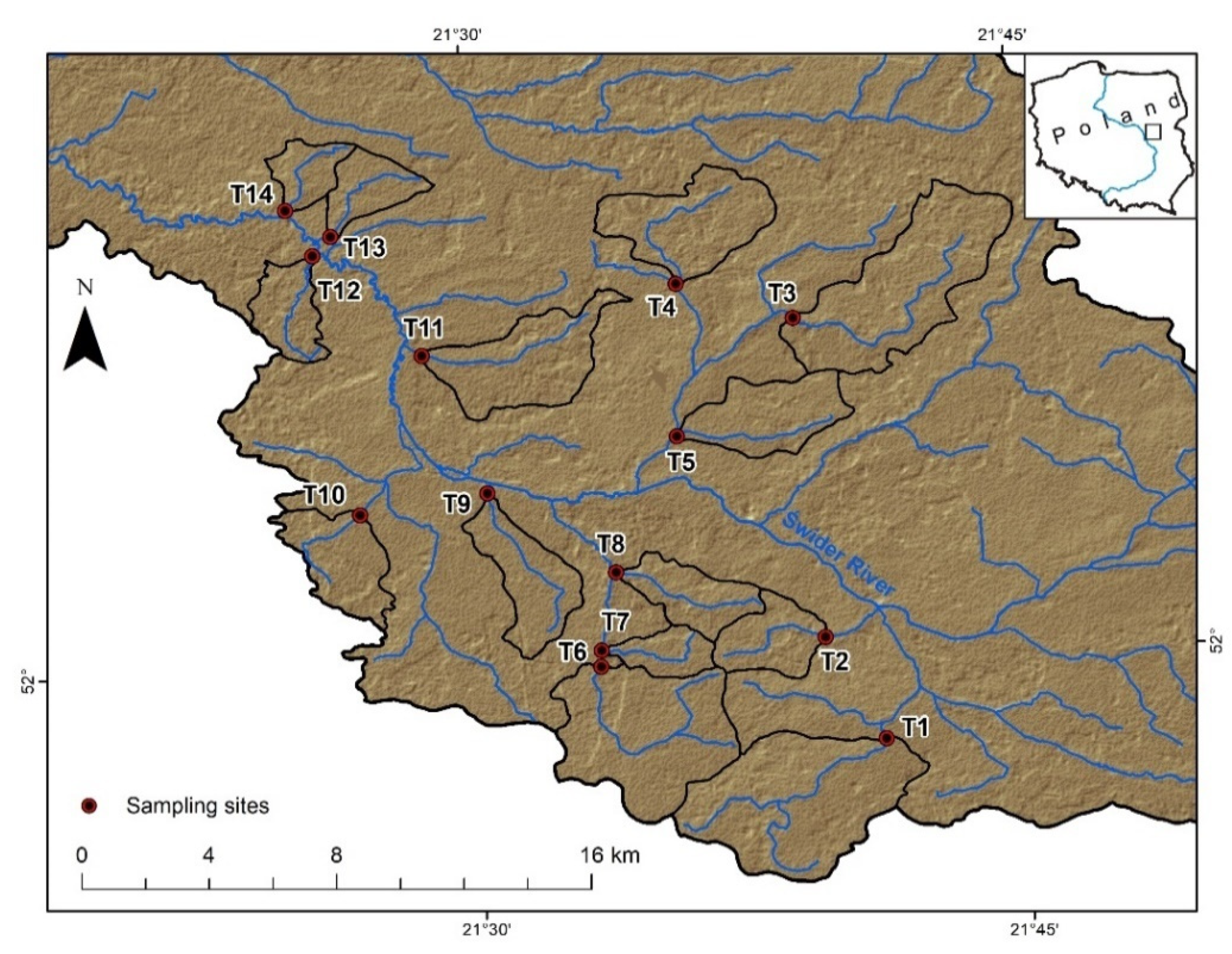
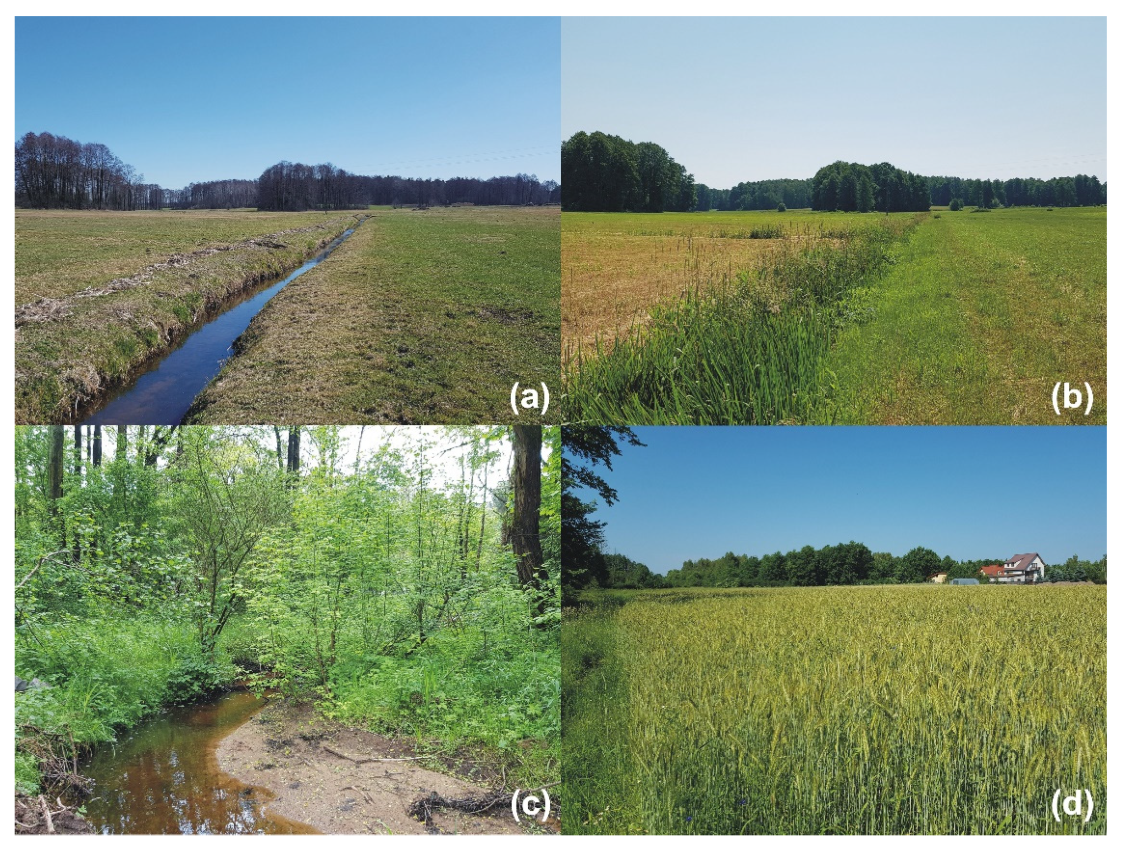
2. Materials and Methods

The investigated area is drained by the Świder River, which is a 99-km-long right tributary of the Vistula River. Its catchment area is approximately 1160.7 km2 (Figure 1) and according to [54], it belongs to the denudation-type Garwolińska Plain, located within the Mazovian Lowland. Superficial deposits from the Quaternary age, building the overall flat plain relief, consist mainly of sandy loam and boulder clays, while in some places aeolian sands and gravels (dune terraces), as well as silt deposits (valleys) are present [55]. The elevation of the study area is relatively uniform and ranges from approximately 108 m a.s.l. (above sea level) near the mouth of the Glinianka Stream to only 187 m a.s.l. near the springs of the Sienniczanka. The climate of the investigated area can be considered as warm temperate in the transitional zone from marine to continental [56]. The mean annual air temperature is approximately 8–9 °C, while annual precipitation amounts to 500–550 mm. The lowest mean temperature is usually observed in January, while the highest in July. The same is true for the highest monthly precipitation sum [57]. As a result, the highest streamflow rates are observed in early spring as a result of snowmelt, and the lowest usually occur during summer and autumn. Because of the agricultural character of the study area, it is dominated by croplands and meadows, while the contribution of forested areas, composed mainly of white willows (Salix alba L.), common aspens (Populus tremula L.), black alders (Alnus glutinosa (L.) Gaertn.), and scots pines (Pinus sylvestris L.), is similar to the average value for Poland (approximately 30%) [58]. It must be emphasized that the investigated area is characterized by a low degree of urbanization—according to the Corine Land Cover 2018, the contribution of anthropogenic areas does not exceed 10%, and such artificial surfaces can be identified as small- and medium-sized villages and settlements.
Field investigations were carried out in twenty independent catchments drained by first- or second-order lowland streams. The sampling sites, with the catchment area ranging from 3.7 to 23.7 km2, were selected with a view to maximizing differences between land cover properties, however, they are simultaneously characterized by relatively similar geological and climatological properties. Their location precluded direct anthropopressure reflected in the water quality, such as point sources related to sewage inflows and unstratified, through-flow reservoirs. Also, the watercourses had to be permanently flowing, which excluded six streams during the sampling period. In consequence, only 14 watercourses were adopted in the analysis (Figure 2).
Water samples were collected from April 2019 to March 2020 in regular monthly intervals (in the middle of each month) into a polyethylene bottles, always from the main current of the streams. Then immediately after transportation to the faculty laboratory, the concentration of nitrate nitrogen (N-NO3) was determined using the sulfanilic acid method, while the phosphate phosphorous concentration (P-PO4) was determined using the molybdenum blue method, both with the use of a LF300 photometer. To determine whether the sampling sites are not directly influenced by anthropopressure during the collection of water samples, dissolved oxygen (DO) saturation (%) and conductivity (µS/cm) were measured in the field. This was conducted with portable, handheld meters Hanna Hi 98193 (resolution of 0.1 °C and ±1.5% mg/L) and Hanna Hi 9811-5 (resolution of ±2.0% µS/cm), both regularly calibrated. Such measurements confirmed the appropriate selection of sampling sites, as the spatial and seasonal variability of DO and conductivity values could be explained by natural factors. Additionally, the macrophytes coverage was assessed in the cross-section of the channels positioned 50, 100, 150, and 200 m upstream from the sampling sites. In such cross-sections, the percentage of macrophytes (from 0 to 100% with 10% of precision) was visually evaluated and then averaged. It must be noted that both measurements and water samples were collected in days characterized by stable flow rates and, whenever possible, a minimum of three days after rainfall events.
To provide a hydrometeorological background, mean monthly air temperature and monthly precipitation sums in the investigated period were presented in the context of the respective mean values from the period of 1991–2020. For this purpose, air temperature and precipitation data from the nearest representative meteorological station Warsaw-Okęcie were acquired from the Institute of Meteorology and Water Management—National Research Institute.
Several catchment metrics were calculated with the use of raster and vector processing tools in ArcMap 10.5 GIS software (Esri, California, USA), to evaluate their influence on the spatial and seasonal variability of N-NO3 and P-PO4 ions in the environment. The catchment area of the sampling sites (A) was estimated with the use of the vector layers of Polish digital hydrographic maps. The contribution of selected, individual types of land cover (in %) were calculated on the basis of two cost-free and European-range datasets. The first, the Corine Land Cover 2018 vector land cover map (CLC 2018), is based predominantly on the visual interpretation of Landsat satellite imagery [59], while the second, the high-resolution Land Cover Map of Europe, is based on automatic classifications of images acquired from the Sentinel 2 satellite (S2GLC), launched by the European Space Agency [60]. Three classes of land cover—agricultural lands, meadows, and forests—were distinguished both from CLC 2018 and S2GLC datasets with the use of vector and raster processing tools. Detailed descriptions of the original classes used to compute them are reported in Table 1. Artificial (anthropogenic) surfaces, marshes, peatbogs, and water bodies were omitted from the analysis due to their sporadic occurrence and, in consequence, their possible disruption of statistical analysis due to many zeros in the dataset. In addition, artificial surfaces were excluded due to significant differences in their contribution across investigated catchments (up to dozens of times).
The contributions of individual land cover types were calculated for the whole catchment area, as well as for buffer zones of 100, 250, and 500 m width, extending from the sampling site upstream to the springs. To determine how land cover distance from the stream influences the relationships between metrics and ion concentrations, the inverse weighted distance method was also applied to calculate metrics. To this end, a modified formula which takes into account the Euclidean distance (ED) of each raster cell to the stream [61] was used:
LC = (SUM [Zi / Di] / SUM [1 / Di]) ×100
where LC is the percentage of land cover type (%); n is the total number of cells in the catchment; Zi (n) is the presence of land cover z in cell n (1 or 0); and Di is the Euclidean distance from cell i to the stream.
To assess the spatial and seasonal variability of nutrient compounds in the investigated lowland catchments, mean, maximum, minimum, and standard deviation of N-NO3 and P-PO4 concentrations were calculated both for the individual sampling sites, as well as for certain months of the sampling period. These values were presented on the mean, max, and min charts. Relationships between the concentration of N-NO3 and P-PO4 and computed land cover metrics were evaluated on the basis of correlation analysis. Initially, data was inspected with the Shaphiro–Wilk goodness of fit test, which indicated that nearly half of the land cover metrics do not have a normal distribution (p < 0.05). After normalization with the logarithmic function, the distribution was still outside of normal. Thus, the Spearman rank correlation coefficient, which is considered as definitely more resistant to outliers and more reliable in the case of a small sample size, was used instead of the Pearson coefficient. In this way land cover types both from CLC 2018 and S2GLC datasets, calculated for the total catchment area, buffer zones, and weighted by Euclidean distance, were linked with the concentration of N-NO3 and P-PO4. This was applied for mean concentration of N-NO3 for the whole investigated period (IV–III) and for the four periods—spring (IV–VI), summer (VII–IX), autumn (X–XII), and winter (I–III), similar to [40,62]. A probability value of correlation of less than 0.05 was considered as statistically significant. Calculations were performed in the Statistica 13.5 software (TIBCO Software Inc., California, USA) and presented in tabular form and on the bar charts, which allowed the authors to characterize seasonal changes in the investigated relationships (Table 2).

3. Results

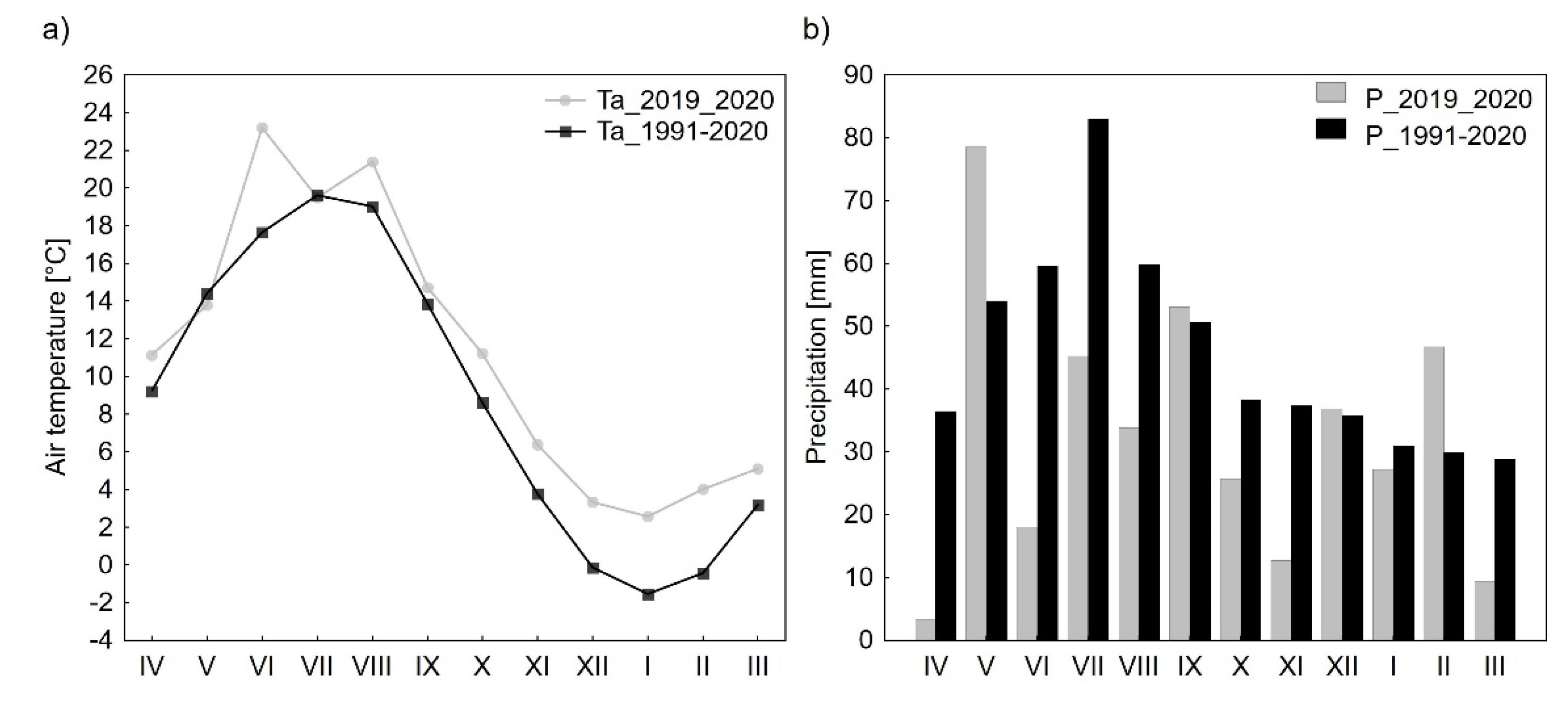
3.1. Hydrometeorological Background

The investigated period from April 2019 to March 2020 can be considered as very warm—the average air temperature at the Warsaw-Okęcie meteorological station reached 11.4 °C, which was 2.5 °C higher than the average from the reference period (1991–2020). The highest mean monthly temperature (21.4 °C) was observed in August, while the lowest in January (2.6 °C). During the sampling period, subzero monthly mean air temperatures were not documented. Furthermore, only in May and July was the air temperature lower than in the reference period (Figure 3a). The precipitation sum during the sampling period was, in turn, definitely lower than in the reference period (Figure 3b), which indicated extremely dry conditions. Total precipitation was only 390 mm, which accounted for only 72% of the average sum of precipitation calculated for the reference period. Except for May, September, December, and February, in the remaining months precipitation was lower than the mean values calculated for the reference period (Figure 3b).

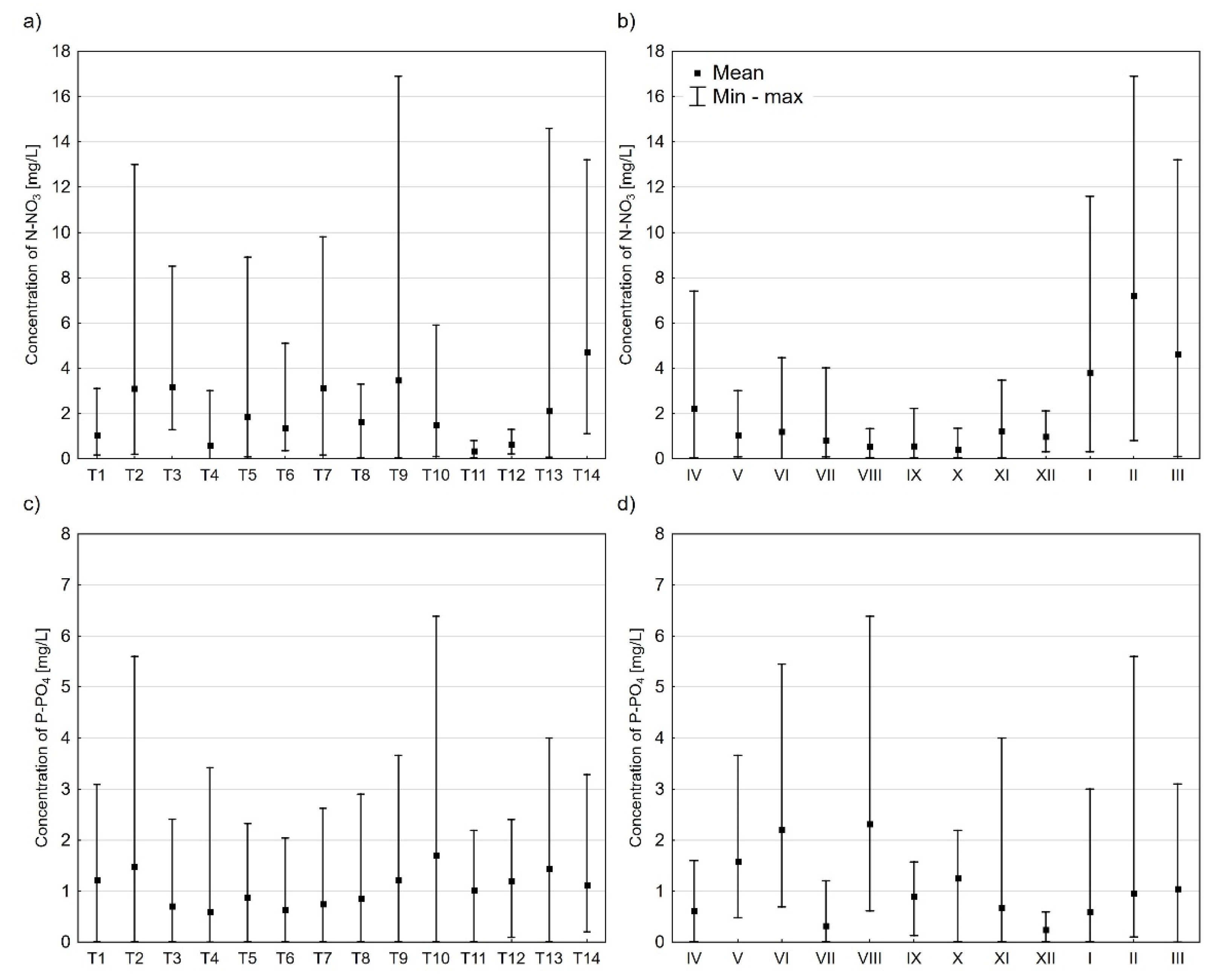
3.2. Spatial and Seasonal Distribution of Nutrients

Clear spatial variability of N-NO3 and P-PO4 concentrations was found between the investigated lowland catchments (Figure 4a–d). In some catchments, the mean and maximum concentrations of N-NO3 did not exceed 1.5 and 2–3 mg/L, respectively, while in other sampling sites values over 15 mg/L were noted, while mean values were definitely higher (Table 3). The variability of N-NO3 concentration measured with the standard deviation was the highest in sampling sites with the highest mean concentration values, such as T2, T9, T13, and T14. In the case of P-PO4, the spatial variability was definitely lower in comparison to N-NO3, while their variability was also generally more aligned across sampling sites, as values of standard deviation ranged from 0.67 to 1.89 mg/L (Table 3).
The seasonal variability of N-NO3 and P-PO4 concentrations was also clearly outlined, as indicated by values from all sampling points, aggregated in the monthly timescale (Figure 4b,d). In the case of N-NO3 relatively low mean and maximum concentrations (not exceed 4.0 mg/L) were mainly observed in the growing season (defined as a period with mean temperature above 5 °C)—particularly from May to as late as December. On the contrary, high values of N-NO3 concentration were noted from January to April, representing winter and early spring months (Figure 4). The seasonal course of P-PO4 concentrations was more complex—high concentrations were interspersed with low ones, which was documented in the summer period. However, in the hot period from May to October generally higher concentrations of P-PO4 were measured in comparison to the winter months (Figure 4).

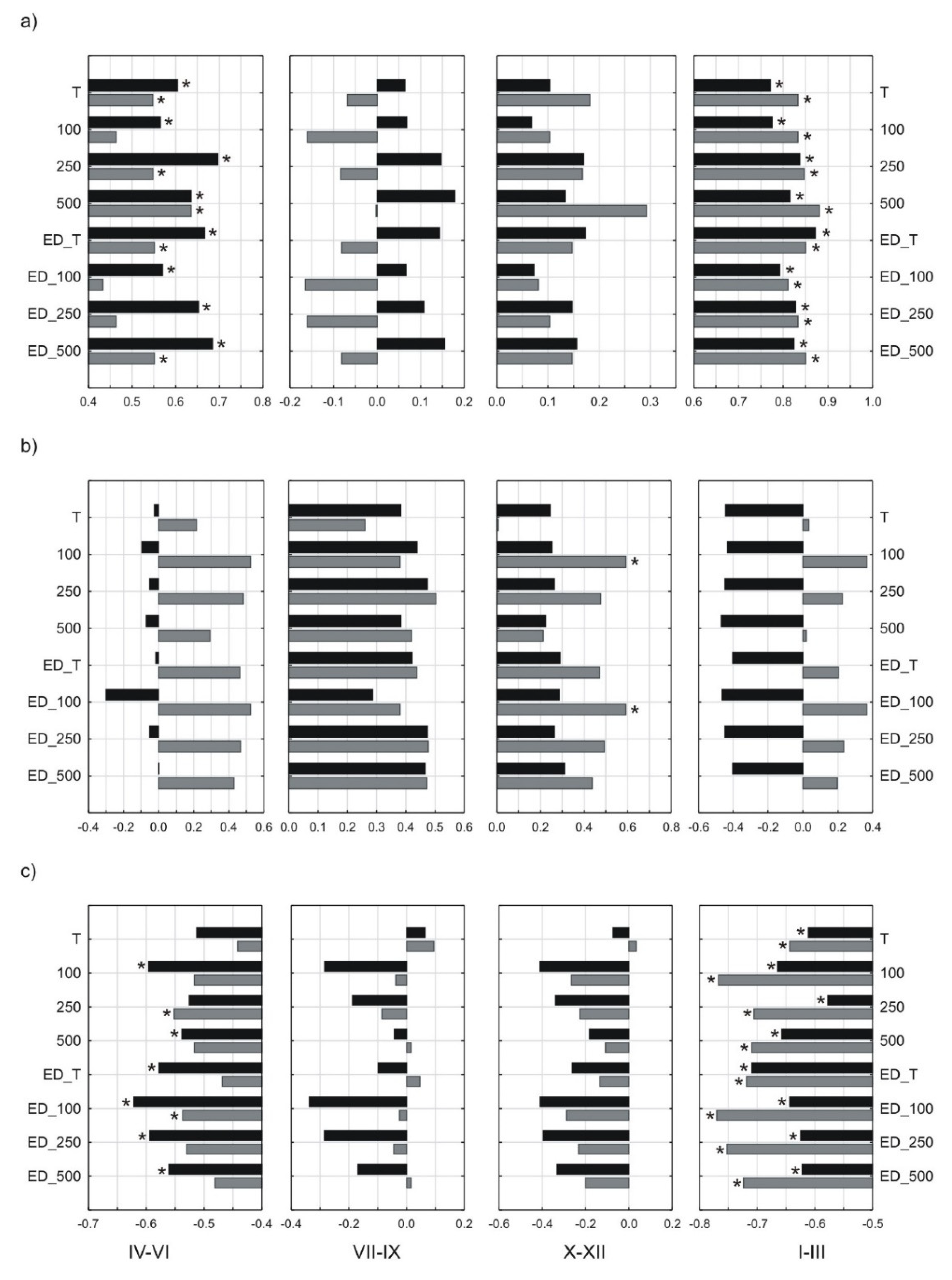
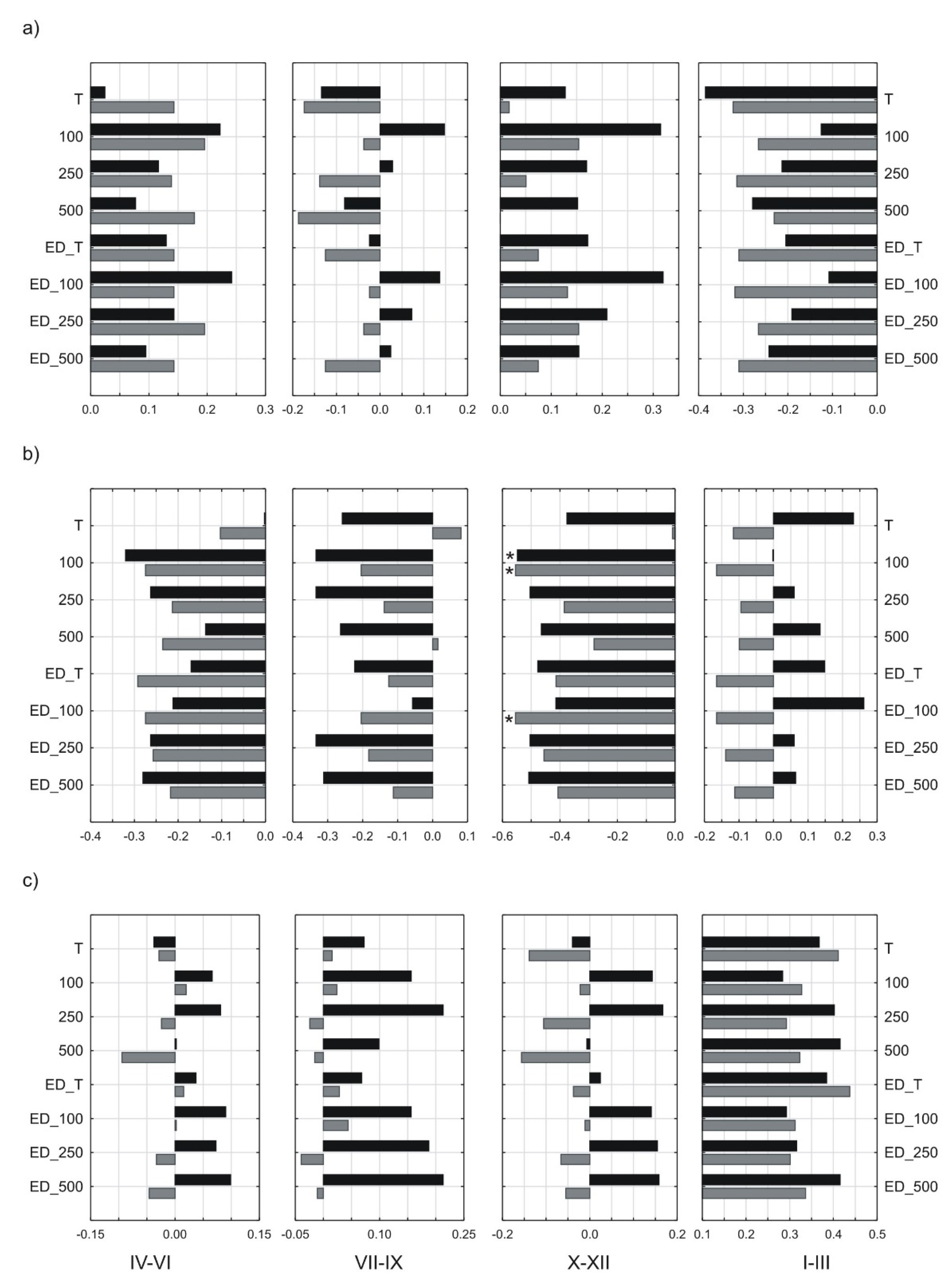
3.3. Land Cover Effects on Nutrient Concentrations

The overall pattern of correlation between selected land cover metrics, calculated for two different datasets, and mean concentrations of N-NO3 and P-PO4 was presented in Table 4. Generally, both in the case of the CLC 2018 and S2GLC datasets, the mean concentration of N-NO3 during the investigated period was positively correlated with the percentage of agricultural lands and negatively correlated with the percentage of forest cover on p < 0.05 (Table 4). For meadow datasets, no statistically significant correlations were found and the relationships, as indicated by the sign of the correlation coefficients, were different depending on the dataset (Table 4). Generally, the CLC 2018 agricultural land and forest datasets provided a slightly better correlation performance with N-NO3 concentrations compared to the respective S2GLC datasets. Across agricultural land datasets, the best performance was found for the larger spatial scales, such as 250-m-wide buffer zones and the total catchment area for CLC 2018 and 500-m-wide buffer zone for S2GLC. The opposite was true for the forest datasets, which were generally better correlated in smaller scales, such as 100-m-wide buffer zones (Table 4). For both land cover datasets, forests were correlated better with N-NO3 concentration with additional Euclidean distance scaling, which was not evidenced for the agricultural lands. In the case of P-PO4 concentration no statistically significant relationships were found with the use of CLC 2018 and S2GLC datasets (p > 0.05) Significant differences in correlation performance, as well as between signs of the correlation, indicate the accidental character of the land cover metrics relationship with P-PO4 concentrations (Table 4).
Changes of the correlation performance across averaged three-month periods provide an insight into the seasonal variability of the land cover effect on N-NO3 concentrations in lowland catchments (Figure 5). Overall, in the case of the agricultural lands dataset, the strongest positive correlation was performed in the winter and spring periods, when nearly all relationships were statistically significant (Figure 5a). The S2GLC agricultural land dataset performance during spring was slightly lower in comparison to CLC 2018 dataset. However, the situation was opposite in the winter period. In the summer and autumn periods, correlation values with agricultural land datasets were insignificant for both CLC 2018 and S2GLC (p > 0.05). Generally speaking, meadows had no significant impact on N-NO3 concentration in the both CLC 2018 and S2GLC datasets (p > 0.05). However, during the autumn period for the buffer zone of 100 m width there was observed single significant positive correlation (Figure 5b). It seems interesting that the S2GLC meadows dataset always provided a positive relationship with N-NO3 concentration, while in the case of the CLC 2018 dataset, the same direction of the impact was noted only in the summer and autumn periods. Additionally, in those seasons the relationship, even not significant, was the strongest. According to the correlation results, the presence of forests generally has a negative impact on N-NO3 concentration for both CLC 2018 and S2GLC datasets in all studied periods (Figure 5c). Positive relationships were documented only in summer and autumn. However, like all of the relationships in those periods, they were found to be statistically insignificant (p < 0.05). The strongest, significant correlations were performed for the CLC 2018 and S2GLC dataset in the winter period. Similar to agricultural lands, in this season the best performance was provided by the S2GLC dataset. This is not true for the spring period, when the CLC 2018 forest dataset performed slightly better. In all periods, the strongest correlations were obtained for the narrowest buffer zones (100 or 250 m), with Euclidean distance scaling.
Correlation performance for the P-PO4 concentration was also seasonally varied, both in the case of agricultural land, meadows, and forest datasets (Figure 6). However, nearly all of the metrics were correlated insignificantly (p < 0.05) and the signs of the correlation varied between the respective CLC 2018 and S2GLC datasets. Only in the case of S2GLC meadows dataset was the direction of the relationships uniform across all of the investigated periods (Figure 6b) and the values of the correlation were relatively higher than for agricultural lands and forests. In the autumn period there was documented an even significant correlation between the P-PO4 concentration and the percentage of meadows in a 100-m-wide buffer zone for both datasets.

4. Discussion

4.1. Spatial and Seasonal Nutrient Dynamics

The effect of land cover on selected nutrient compounds was investigated on the example of lowland agricultural catchments located in central Poland. The sampling period was characterized by unusually hot and dry meteorological conditions compared to the long-term averages. Such conditions have a significant effect on ion sources, migration, and delivery processes in geochemical pools [63]. Nevertheless, clear seasonal and spatial patterns of nitrate and phosphate concentration were observed in the investigated sites. Overall, seasonal changes of N-NO3 concentrations were generally consistent with the typical annual cycle, as documented and discussed previously [64,65,66]. However, low values of N-NO3 concentrations were also documented during autumn, with the minimum values observed as late as in October. Such a clear shift in the annual concentration course can be explained by increased air temperature in the autumn months, even by as much as 3.5 °C in December in comparison to the reference period. Simultaneously, small precipitation totals in this period resulted in a slower rate of N-NO3 ion migration. In comparison to values reported in the literature [67,68], in the studied sites a relatively low concentration of N-NO3 during the summer was observed, as well as its low spatial variability. This could be related to nutrient uptake, especially by the well-developed macrophytes [69], which is an effective process at low flow velocities [70]. In fact, in some of the investigated streams (e.g. T5, T7, T9, and T13), channel beds and banks were locally overgrown by Sagittaria sagittifolia L., Phragmites australis (Cav.) Trin. ex Steud., Sparganium erectum L., and Carex nigra Reichard. In addition, such streams were characterized by greater seasonal variability of N-NO3 than forested, solar-sheltered catchments, where macrophytes occurred only locally (e.g. T8, T10, and T11). Denitrification, which is generally effective in quasi-natural streams in the presence of moderate water temperatures, could also constitute an important process of N-NO3 removal [71]. In the case of P-PO4, seasonal changes of its concentrations were significantly different in comparison to N-NO3. They could be mainly related with hydrological conditions, as during the summer period the concentration of P-PO4 was definitely higher than in the autumn and winter periods. During such summer baseflow periods, as documented by [72], inorganic soluble phosphorus becomes a significant component in the total phosphorous budget. A decrease of P-PO4 concentration as an effect of dilution was particularly visible in July and September, when higher streamflow rate was observed due to intensive rainfall events occurred two and three days before sampling. In can be supposed that such dynamics of P-PO4 after storm events is characteristic for the lowland landscape, where soil and land erosion, the main natural source of P-PO4 ion [73,74], is expected to be insignificant due to slight slopes and generally flat terrain. The presented seasonal variability of P-PO4 concentrations, even reported previously in the literature [75,76,77] is not the dominant, typical pattern, as different seasonal P-PO4 variability was also observed [78,79]. In fact, seasonal changes of N-NO3 and P-PO4 concentrations in the investigated lowland streams are differently driven. In the case of N-NO3 ions, temporal variability mainly results from the biogeochemical activity of terrestrial and aquatic vegetation, while in the case of P-PO4 ions, a clear dependence on hydrological conditions was documented. A similar response of nutrient dynamics to landscape and hydrometeorogical conditions was previously reported by [80] in the Owasco Lake catchment in Northeastern USA.

4.2. Land Cover Effect on Nutrient Variability

Results of the correlation analysis confirmed that agricultural activity has a great impact on N-NO3 released into lowland streams. The positive correlation of the contribution of agricultural lands metrics in the catchment areas and N-NO3 concentration was also extensively documented for other geographical regions [22,34,81,82,83]. On the other hand, the presence of deciduous and coniferous forests resulted in the decrease of the N-NO3 delivered to the watercourses, which could be linked with ion uptake and its retention by woodland vegetation [84,85,86]. However, in the current study, the landscape effect on ion concentration was dependent on the season, both for the agricultural lands and forests. The contribution of agricultural lands and forests was significantly correlated with N-NO3 concentration only in the spring and winter periods. This seasonal tendency can be related to the limited uptake of the N-NO3 ions due to the lack of herbaceous and crop vegetation in this period [66] and increased hydrological connectivity caused by rain or snow precipitation [87], enhanced by low evapotranspiration [88]. Artificial and natural fertilizers, used frequently by farmers, constitute additional sources of nitrogen ions in this period [51,89]. Another factor worth mentioning are decomposition processes of terrestrial vegetation and macrophytes [90], as well as leaf litter from riparian zones [91]. In the spring and summer months, when terrestrial and aquatic vegetation is responsible for an uptake in nutrients, low and more uniform intensity of ion fluxes was observed through the catchments. In the case of P-PO4, the lack of significant relationships between its concentrations and landscape metrics can be explained by the combination of several factors. Apart from the clear dependence of P-PO4 on hydrological conditions, low intensity of soil and land erosion seems to be crucial in such lowland catchments. Moreover, because most of the rural areas in the investigated catchments are not connected to the sanitary sewer, human activity can be an important external source of P-PO4 ions. This was previously evidenced in the neighboring Wilga catchment by [50] and can be confirmed by the increased P-PO4 concentrations in comparison to other investigated lowland catchments. During spring and summer, [53] found that the P-PO4 concentration in three Pomeranian streams always remains below 0.5 mg/L, while in the case of the Mazovian Raszynka River, the maximum annual concentration of P-PO4 only amounted to 0.83 mg/L [52]. It is worth noting that a weak correlation of the phosphorous concentrations in streams with land cover types was also reported for agricultural catchments in other geographical regions [49].
The performance of land cover metrics in water quality prediction, calculated for different spatial scales with even additional distance of flow accumulation scaling, was previously broadly discussed [42,45,92]. However, the presented results are not clear and unequivocal. For example, [81] reported that the concentration of nitrates in the studied watercourses can be equally justified by land use in the whole catchment area and in the 100-m-wide buffer zone. Different conclusions were presented by [64] and indicated that landscape characteristics of the whole catchment area were of greater importance than the characteristics of the buffer zone. In other studies, 100-meter-wide [41] and 300-meter-wide [93] buffer zones were found to be the most accurate in terms of predicting river water quality. In the current study, the use of buffer zones usually increased the performance of the correlation for mean N-NO3 concentration in lowland streams, both for the CLC 2018 and the S2GLC datasets. The application of Euclidean distance in the calculation of metrics resulted in the further increase of the correlation performance, but this effect was widely present only for the forest datasets. In the case of agricultural lands dataset, an increase of the correlation coefficient value after distance weighting was only observed for the total catchment area—the difference in the performance level for buffer zone metrics (100, 250, and 500 m) was negligible or even opposite. Moreover, the performance differentiation between agricultural lands and forests became apparent depending on spatial scale. The highest correlation performance for agricultural lands datasets was reported generally for the widest buffer zone (500 m), as well as the total catchment area. Meanwhile, the presence of the forests was the most important in the narrowest buffer zone (100 m), with additional Euclidean distance weighting. This different performance tendency between land cover types can be explained by their physical nature. The forest cover effect on water quality is the most important in the closest proximity to the stream, where ion uptake, denitrification, and sediment trapping occur [94,95]. On the other hand, the influence of agricultural lands is greater, the larger the area of their drainage. Some of the previous studies also indicated that even with the same land use percentage, landscape configuration, measured with the patch density, edge density, and mean shape index, plays an important role in organic matter and nutrient runoff from catchments [39]. However, this can be more important in larger catchments, where their area is suggested to have a significant effect on metrics performance [42].
In the current study, there was also the possibility to compare metrics performance calculated on the basis of the two independent datasets, both widely accessible for nearly all of the European countries [59,60]. Overall, both CLC 2018 and S2GLC datasets provided similar correlation performance and the differences in significant correlation values usually did not exceed 0.05–0.1. However, it is worth noting that metrics based on S2GLC dataset were better correlated in smaller spatial scales, such as buffer zones of 100 and 250 m width. At such scales, high-resolution datasets seem to be favorable, although this cannot be stated for larger areas. Finally, although the results of the correlation analysis for meadows were not significant, the opposite impact of this land cover type on N-NO3 between used datasets was observed, both for the whole study period and for specific seasons. The contribution of meadows in S2GLC dataset was definitely higher, marking in that way a small participation of agricultural lands in the comparison to the CLC 2018. This indicates that the classification algorithm in the S2GLC dataset classified some agricultural lands as meadows. Moreover, this example suggests that great carefulness is needed when evaluating the impact of meadows on water quality, as it could be overestimated in both ways. Meadows identified from the aerial or satellite level can in fact be different in their functioning, that is, grazed, fertilized, and mowed. In addition, sometimes they are not managed in any way, which makes their functioning much more similar to natural herbaceous vegetation [96]. This is reflected in their impact on water quality, which could be significantly different: from being an additional source of nutrient ions [97] to acting as a biogeochemical barrier [52]. Therefore, uncritical reliance on satellite-based datasets could lead to potentially erroneous conclusions if there is no precise information about such land cover management.

4.3. Implications for Water Quality Management

Understanding the complex relationships observed between terrestrial and aquatic environments is definitely required in appropriate management of lotic ecosystems. The obtained results provided new insight into this subject and could be representative of the other lowland agricultural catchments in the temperate climate, characterized by flat terrain and low hydrological connectivity. Overall, statistical modelling conducted on the basis of landscape predictors should take into account the strong seasonal variability of their impact, driven mainly by vegetation cover changes. As indicated, land cover metrics during summer and autumn seasons could be useless. Nevertheless, this fact points to the need to search for new predictors, which could explain nutrients variability during growing season, and such additional variables could include macrophytes density, as well as soil properties metrics [42]. Moreover, from scaling (weighting) methods presented in the literature [47,98,99], the use of buffer zones and/or Euclidean distance scaling seems to be the optimal solution for modelling purposes in lowland landscapes. Flow accumulation scaling could be difficult to apply due to blind drainage, similar to slope scaling in terms of small differences in elevation and low steeper slopes. Finally, correlation values reported for metrics based on the S2GLC dataset (10 m/pixel) and CLC 2018 dataset (minimum width of objects: 100 m) indicated that the increase of data resolution had not significantly improved modeling performance. This is an important issue in the context of the cost- and time-efficiency of investigations. It can be supposed that using high-resolution land cover maps acquired from photogrammetric low-altitudes flights could be justified only for small experimental catchments, while in such studied mesoscale catchments widely available and cost-free datasets can be used with high efficiency. Meanwhile, the results of the correlation analysis confirm the previous findings [62,95] and suggest that restoring riparian buffer zones covered with trees and woodland vegetation would have a clear impact on the N-NO3 reduction in lowland streams. According to [94], a 30–40-meters-wide buffer zone can effectively protect the physical, chemical, and biological integrity of small streams. However, management in such streams also requires the appropriate treatment of macrophytes, such as periodic planting and cutting, as they are responsible for different effects depending on the season. Maintaining good water quality of small lowland streams is crucial not only in terms of environmental protection, but also ecology and fisheries management, as they act as a refuges for riverine species, especially valuable freshwater fish [100,101].

5. Conclusions

The effect of the land cover on selected nutrient dynamics was investigated in fourteen temperate lowland catchments in central Poland. Generally, a clear spatial and seasonal variability of N-NO3 and P-PO4 concentration was observed in the studied catchments, which could be mainly related with the vegetation cycle and hydrological conditions, respectively. For both the CLC 2018 and S2GLC datasets, the percentage of agricultural lands was found to have a significant positive association with N-NO3 concentration, while the forest percentage was negatively linked with the level of nitrates. However, significant relationships were only found in the spring and winter periods, when ion release from decomposing vegetation and higher hydrological connectivity occur. Meanwhile, the effect of meadows on N-NO3 was usually not significant and its direction was dependent on the land cover dataset. The use of buffer zones usually increased the correlation performance of agricultural land and forest datasets, whereas Euclidean distance scaling improved such performance mainly in the case of forest cover metrics. Overall, the total catchment area and 500-m-wide buffer zone provided the best correlation for agricultural lands, which was opposite to forests, appeared to be the most significant in the 100-m-wide buffer zone. In contrast, P-PO4 concentrations were generally not significantly related with any land cover metrics. The study highlighted the importance of understanding of relationship between land cover and stream nutrient concentrations, as well as evaluating the performance of different metrics scales and datasets in such a prediction for practical implications.

Author Contributions

Conceptualization: M.Ł.; methodology: M.Ł.; formal analysis: M.Ł. and M.F.; investigation: M.Ł., M.F., S.G., Z.K., P.M., J.M., and W.Z.; resources: M.Ł.; writing—original draft preparation: M.Ł. and M.F.; writing—review and editing: M.Ł., M.F., S.G., Z.K., P.M., J.M., and W.Z.; visualization: M.Ł. and M.F. All authors have read and agreed to the published version of the manuscript.

Funding

This research was funded by the Faculty of Geography and Regional Studies, University of Warsaw, grant number SOP-I-53/19 and SWIB 6/2021.

Data Availability Statement

Not applicable.

Acknowledgments

The authors thank the two anonymous reviewers for their helpful and constructive comments.

Conflicts of Interest

The authors declare no conflict of interest.

References

  1. Smith, V.H.; Tilman, G.D.; Nekola, J.C. Eutrophication: Impacts of excess nutrient inputs on freshwater, marine and terrestrial ecosystems. Environ. Pollut. 1999, 100, 176–196. [Google Scholar] [CrossRef]
  2. Schindler, D.W. Recent advances in the understanding and management of eutrophication. Limnol. Oceanogr. 2006, 51, 356–363. [Google Scholar] [CrossRef] [Green Version]
  3. Chislock, M.F.; Doster, E.; Zitomer, R.A.; Wilson, A.E. Eutrophication: Causes, consequences, and controls in aquatic ecosystems. Nature Educ. Knowledge 2013, 4, 10. [Google Scholar]
  4. Romanowska-Duda, Z.; Mankiewicz, J.; Tarczyńska, M.; Walter, Z.; Zalewski, M. The effect of toxic cyanobacteria (blue-green algae) on water plants and animal cells. Pol. J. Environ. Stud. 2002, 11, 561–566. [Google Scholar]
  5. Heisler, J.; Glibert, P.; Burkholder, J.; Anderson, D.; Cochlan, W.; Dennison, W.; Gobler, C.; Dortch, Q.; Heil, C.; Humphries, E.; et al. Eutrophication and harmful algal blooms: A scientific consensus. Harmful Algae 2008, 8, 3–13. [Google Scholar] [CrossRef] [PubMed] [Green Version]
  6. Mankiewicz-Boczek, J.; Palus, J.; Gągała, I.; Izydorczyk, K.; Jurczak, T.; Dziubałtowska, E.; Stępnik, M.; Arkusz, J.; Komorowska, M.; Skowron, A.; et al. Effects of microcystins-containing cyanobacteria from a temperate ecosystem on human lymphocytes culture and their potential for adverse human health effects. Harmful Algae 2011, 10, 356–365. [Google Scholar] [CrossRef]
  7. Smith, R.A.; Alexander, R.B.; Schwarz, G.E. Natural background concentrations of nutrients in streams and rivers of the conterminous United States. Environ. Sci. Techol. 2003, 37, 3039–3047. [Google Scholar] [CrossRef] [Green Version]
  8. Dorgham, M. Effects of eutrophication. In Eutrophication: Causes, Consequences and Control, 1st ed.; Ansari, A., Gill, S., Eds.; Springer: Dordrecht, The Netherlands, 2014; Volume 2, pp. 29–44. [Google Scholar]
  9. Camargo, J.A.; Alonso, A. Ecological and toxicological effects of inorganic nitrogen pollution in aquatic ecosystems: A global assessment. Environ. Int. 2006, 32, 831–849. [Google Scholar] [CrossRef] [PubMed]
  10. Lewis, W.M.; Morris, D.P. Toxicity of nitrite to fish: A review. Trans. Am. Fish. Soc. 1986, 115, 183–195. [Google Scholar] [CrossRef]
  11. Cheng, W.; Chen, J.C. The virulence of Enterococcus to freshwater prawn Macrobrachium rosenbergii and its immune resistance under ammonia stress. Fish Shellfish Immunol. 2002, 12, 97–109. [Google Scholar] [CrossRef] [PubMed]
  12. Nash, L. Water quality and health. In Water in Crisis: A Guide to the World’s Fresh Water Resources, 1st ed.; Gleik, P.H., Ed.; Oxford University Press: New York, NY, USA, 1993; pp. 25–39. [Google Scholar]
  13. Alonso, A.; Camargo, J.A. Short-term toxicity of ammonia, nitrite, and nitrate to the aquatic snail Potamopyrgus antipodarum (Hydrobiidae, Mollusca). Bull. Environ. Contam. Toxicol. 2003, 70, 1006–1012. [Google Scholar] [CrossRef]
  14. Camargo, J.A.; Alonso, A.; Salamanca, A. 2005 Nitrate toxicity to aquatic animals: A review with new data for freshwater invertebrates. Chemosphere 2005, 58, 1255–1267. [Google Scholar] [CrossRef]
  15. Granger, S.J.; Bol, R.; Anthony, S.; Owens, P.N.; White, S.M.; Haygarth, P.M. Towards a holistic classification of diffuse agricultural water pollution from intensively managed grasslands on heavy soils. In Advances in Agronomy, 1st ed.; Sparks, D.L., Ed.; Elsevier: Burlington, MA, USA, 2010; Volume 105, pp. 83–115. [Google Scholar]
  16. Lintern, A.; Webb, J.A.; Ryu, D.; Liu, S.; Bende-Michl, U.; Waters, D.; Leahy, P.; Wilson, P.; Western, W. Key factors influencing differences in stream water quality across space. WIREs Water 2018, 5, e1260. [Google Scholar] [CrossRef] [Green Version]
  17. Gasiūnas, V.; Lysoviene, J. Nutrient retention efficiency of small regulated streams during the season of low-flow regime in Central Lithuanian lowland. Hydrol. Res. 2014, 45, 357–367. [Google Scholar] [CrossRef]
  18. Bączyk, A.; Wagner, M.; Okruszko, T.; Grygoruk, M. Influence of technical maintenance measures on ecological status of agricultural lowland rivers–Systematic review and implications for river management. Sci. Total Environ. 2018, 627, 189–199. [Google Scholar] [CrossRef] [PubMed]
  19. McGrane, S.J. Impacts of urbanisation on hydrological and water quality dynamics and urban water management: A review. Hydrol. Sci. J. 2016, 61, 2295–2311. [Google Scholar] [CrossRef]
  20. Blaszczak, J.R.; Delesantro, J.M.; Zhong, Y.; Urban, D.L.; Bernhardt, E.S. Watershed urban development controls on urban streamwater chemistry variability. Biogeochemistry 2019, 144, 61–84. [Google Scholar] [CrossRef]
  21. Driscoll, C.T.; Whitall, D.; Aber, J.; Boyer, E.W.; Castro, M.; Cronan, C.; Goodale, C.L.; Groffman, P.M.; Hopkinson, C.; Lambert, K.; et al. Nitrogen pollution in the Northeastern United States: Sources, effects, and management options. Bioscience 2003, 53, 357–374. [Google Scholar] [CrossRef]
  22. Poor, C.J.; McDonnell, J.J. The effects of land use on stream nitrate dynamics. J. Hydrol. 2007, 332, 54–68. [Google Scholar] [CrossRef]
  23. Edwards, A.C.; Withers, P.J.A. Transport and delivery of suspended solids, nitrogen and phosphorus from various sources to freshwaters in the UK. J. Hydrol. 2008, 350, 144–153. [Google Scholar] [CrossRef]
  24. Agouridis, C.T.; Workman, S.R.; Warner, R.C.; Jennings, G.D. Livestock grazing management impacts on stream water quality: A review. J. Am. Water Resour. Assoc. 2005, 41, 591–606. [Google Scholar] [CrossRef]
  25. Żelazny, M.; Pufelska, M.; Sajdak, M.; Jelonkiewicz, Ł.; Bukowski, M. Wpływ rozpadu drzewostanu w Tatrzańskim Parku Narodowym na zróżnicowanie przestrzenne stężenia azotanów. Acta Sci. Pol. Formatio Circumiectus 2019, 18, 149–161. [Google Scholar] [CrossRef]
  26. Pärn, J.; Mander, Ü. Landscape factors of nutrient transport in temperate agricultural catchments. WIT Trans. Ecol. Environ. 2007, 104, 411–423. [Google Scholar]
  27. Heathwaite, A.L. Multiple stressors on water availability at global to catchment scales: Understanding human impact on nutrient cycles to protect water quality and water availability in the long term. Freshw. Biol. 2010, 55, 241–257. [Google Scholar] [CrossRef]
  28. Soranno, P.A.; Cheruvelil, K.S.; Wagner, T.; Webster, K.E.; Bremigan, M.T. Effects of land use on lake nutrients: The importance of scale, hydrologic connectivity, and region. PLoS ONE 2015, 10, e0135454. [Google Scholar] [CrossRef] [PubMed] [Green Version]
  29. Billmire, M.; Koziol, B.W. Landscape and flow path-based nutrient loading metrics for evaluation of in-stream water quality in Saginaw Bay, Michigan. J. Great Lakes Res. 2018, 44, 1068–1080. [Google Scholar] [CrossRef]
  30. Šaulys, V.; Survilė, O.; Stankevičienė, R. An assessment of self-purification in streams. Water 2020, 12, 87. [Google Scholar] [CrossRef] [Green Version]
  31. Vidon, P.G.; Hill, A.R. A landscape-based approach to estimate riparian hydrological and nitrate removal functions. J. Am. Water Resour. Assoc. 2006, 42, 1099–1112. [Google Scholar] [CrossRef]
  32. Liu, X.; Mang, X.; Zhang, M. Major factors influencing the efficacy of vegetated buffers on sediment trapping: A review and analysis. J. Environ. Qual. 2008, 37, 1667–1674. [Google Scholar] [CrossRef]
  33. Fatehi, I.; Amiri, B.J.; Alizadeh, A.; Adamowski, J. Modeling the relationship between catchment attributes and in-stream water quality. Water Resour. Manag. 2015, 29, 5055–5072. [Google Scholar] [CrossRef]
  34. Hill, A.R. Factors affecting the export of nitrate-nitrogen from drainage basins in Southern Ontario. Water Res. 1978, 12, 1045–1057. [Google Scholar] [CrossRef]
  35. Uuemaa, A.; Antrop, M.; Roosaare, J.; Marja, R.; Mander, Ü. Landscape metrics and indices: An overview of their use in landscape research. Living Rev. Landsc. Res. 2009, 3, 1–28. [Google Scholar] [CrossRef]
  36. Griffith, J. Geographic techniques and recent applications of remote sensing to landscape-water quality studies. Water Air Soil Pollut. 2002, 138, 181–197. [Google Scholar] [CrossRef]
  37. Ramadas, M.; Samantaray, A.K. Applications of remote sensing and GIS in water quality monitoring and remediation: A state-of-the-art review. In Water Remediation. Energy, Environment, and Sustainability, 1st ed.; Bhattacharya, S., Gupta, A., Gupta, A., Pandey, A., Eds.; Springer: Singapore, 2018; pp. 225–246. [Google Scholar]
  38. Jones, K.B.; Neale, A.C.; Nash, M.S.; Van Remortel, R.D.; Wickham, J.D.; Riitters, K.H.; O’Neill, R.V. Predicting nutrient and sediment loadings to streams from landscape metrics: A multiple watershed study from the United States Mid-Atlantic Region. Landsc Ecol. 2001, 16, 301–312. [Google Scholar] [CrossRef]
  39. Uuemaa, E.; Roosaare, J.; Mander, Ü. Landscape metrics as indicators of river water quality at catchment scale. Nord. Hydrol. 2007, 38, 125–138. [Google Scholar] [CrossRef]
  40. Sliva, L.; Williams, D.D. Buffer zone versus whole catchment approaches to studying land use impact on river water quality. Water Res. 2001, 35, 3462–3472. [Google Scholar] [CrossRef]
  41. Ou, Y.; Wang, X.; Wang, L.; Rousseau, A.N. Landscape influences on water quality in riparian buffer zone of drinking water source area, Northern China. Environ. Earth Sci. 2016, 75, 1–13. [Google Scholar] [CrossRef]
  42. Staponites, L.R.; Barták, V.; Bílý, M.; Simon, O.P. Performance of landscape composition metrics for predicting water quality in headwater catchments. Sci. Rep. 2019, 9, 14405. [Google Scholar] [CrossRef] [PubMed]
  43. Castillo, M.M. Land use and topography as predictors of nutrient levels in a tropical catchment. Limnologica 2010, 40, 322–329. [Google Scholar] [CrossRef] [Green Version]
  44. Hu, X.; Wang, H.; Zhu, Y.; Xie, G.; Shi, H. Landscape characteristics affecting spatial patterns of water quality variation in a highly disturbed region. Int. J. Environ. Res. Public Health 2019, 16, 2149. [Google Scholar] [CrossRef] [Green Version]
  45. Huang, W.; Mao, J.; Zhu, D.; Lin, C. Impacts of land use and land cover on water quality at multiple buffer-zone scales in a Lakeside City. Water 2020, 12, 47. [Google Scholar] [CrossRef] [Green Version]
  46. Liu, Z.; Li, Y.; Li, Z. Surface water quality and land use in Wisconsin, USA—a GIS approach. J. Integr. Environ. Sci. 2009, 6, 69–89. [Google Scholar] [CrossRef]
  47. Medupin, C.; Bark, R.; Owusu, K. Land cover and water quality patterns in an urban river: A case study of river Medlock, Greater Manchester, UK. Water 2020, 12, 848. [Google Scholar] [CrossRef] [Green Version]
  48. Krupa, M.; Tate, K.W.; van Kessel, C.; Serwar, N.L.; Linquist, B.A. Water quality in rice-growing catchments in a Mediterranean climate. Agric. Ecosyst. Environ. 2011, 144, 290–301. [Google Scholar] [CrossRef]
  49. Wang, Y.; Li, Y.; Liu, X.; Liu, F.; Li, Y.; Song, L.; Li, H.; Ma, Q.; Wu, J. Relating land use patterns to stream nutrient levels in red soil agricultural catchments in subtropical central China. Environ. Sci. Pollut. Res. 2014, 21, 10481–10492. [Google Scholar] [CrossRef]
  50. Suchożebrski, J. A method for assessing the conditions of migration of pollutants to the groundwater on the agriculturally used lowland areas. Misc. Geogr. 2002, 10, 175–184. [Google Scholar] [CrossRef] [Green Version]
  51. Lawniczak, A.E.; Zbierska, J.; Nowak, K.; Achtenberg, K.; Grześkowiak, A.; Kanas, K. Impact of agriculture and land use on nitrate contamination in groundwater and running waters in central-west Poland. Environ. Monit. Assess. 2016, 188, 172–189. [Google Scholar] [CrossRef] [Green Version]
  52. Burzyńska, I. Monitoring of selected fertilizer nutrients in surface waters and soils of agricultural land in the river valley in Central Poland. J. Water Land Dev. 2019, 43, 41–48. [Google Scholar] [CrossRef] [Green Version]
  53. Matej-Lukowicz, K.; Wojciechowska, E.; Nawrot, N.; Dzierzbicka-Głowacka, L.A. Seasonal contributions of nutrients from small urban and agricultural watersheds in Northern Poland. PeerJ 2020, 8, e8381. [Google Scholar] [CrossRef]
  54. Kondracki, J. Geografa regionalna Polski, 3rd ed.; PWN: Warsaw, Poland, 2002. [Google Scholar]
  55. Nowakowski, E. Physiographical characteristics of Warsaw and the Mazovian Lowland. Memorabilia Zool. 1981, 34, 13–31. [Google Scholar]
  56. Somorowska, U.; Łaszewski, M. Human-influenced streamflow during extreme drought: Identifying driving forces, modifiers, and impacts in an urbanized catchment in Central Poland. Water Environ. J. 2017, 31, 345–352. [Google Scholar] [CrossRef]
  57. Wrzesiński, D. Reżimy rzek Polski. In Hydrologia Polski, 1st ed.; Jokiel, P., Marszelewski, W., Pociask-Karteczka, J., Eds.; PWN: Warsaw, Poland, 2017; pp. 215–221. [Google Scholar]
  58. Banach, J.; Skrzyszewska, K.; Skrzyszewski, J. Reforestation in Poland: History, current practice and future perspectives. REFORESTA 2017, 3, 185–195. [Google Scholar] [CrossRef] [Green Version]
  59. Rosina, K.; Batista e Silva, F.; Vizcaino, P.; Marín Herrera, M.; Freire, S.; Schiavina, M. Increasing the detail of European land use/cover data by combining heterogeneous data sets. Int. J. Digit. Earth 2020, 13, 602–626. [Google Scholar] [CrossRef]
  60. Malinowski, R.; Lewiński, S.; Rybicki, M.; Gromny, E.; Jenerowicz, M.; Krupiński, M.; Nowakowski, A.; Wojtkowski, C.; Krupiński, M.; Krätzschmar, E.; et al. Automated production of a land cover/use map of Europe based on Sentinel-2 imagery. Remote Sens. 2020, 12, 3523. [Google Scholar] [CrossRef]
  61. Grabowski, Z.J.; Watson, E.; Chang, H. Using spatially explicit indicators to investigate watershed characteristics and stream temperature relationships. Sci. Total Environ. 2016, 551–552, 376–386. [Google Scholar] [CrossRef] [Green Version]
  62. Clune, J.W.; Crawford, J.K.; Chappell, W.T.; Boyer, E.W. Differential effects of land use on nutrient concentrations in streams of Pennsylvania. Environ. Res. Commun. 2020, 2, 115003. [Google Scholar] [CrossRef]
  63. Mosley, L.M. Drought impacts on the water quality of freshwater systems: Review and integration. Earth Sci. Rev. 2015, 40, 203–214. [Google Scholar] [CrossRef]
  64. Martin, C.; Aquilina, L.; Gascuel-Odoux, C.; Molénat, J.; Faucheux, M.; Ruiz, L. Seasonal and interannual variations of nitrate and chloride in stream waters related to spatial and temporal patterns of groundwater concentrations in agricultural catchments. Hydrol. Process. 2004, 18, 1237–1254. [Google Scholar] [CrossRef]
  65. Howden, N.J.K.; Burt, T.P.; Worrall, F.; Whelan, M.J.; Bieroza, M. Nitrate concentrations and fluxes in the River Thames over 140 years (1868–2008): Are increases irreversible? Hydrol. Process. 2010, 24, 2657–2662. [Google Scholar] [CrossRef]
  66. Górski, J.; Dragon, K.; Kaczmarek, P.M.J. Nitrate pollution in the Warta River (Poland) between 1958 and 2016: Trends and causes. Environ. Sci. Pollut. Res. 2019, 26, 2038–2046. [Google Scholar] [CrossRef] [Green Version]
  67. Skorbiłowicz, M.; Ofman, P. Seasonal changes of nitrogen and phosphorus concentration in Supraśl. J. Ecol. Eng. 2014, 15, 26–31. [Google Scholar]
  68. McIsaac, G.F.; David, M.B.; Gertner, G.Z. Illinois river nitrate-nitrogen concentrations and loads: Long-term variation and association with watershed nitrogen inputs. J. Environ. Qual. 2016, 45, 1268–1275. [Google Scholar] [CrossRef] [Green Version]
  69. Birgand, F.; Skaggs, R.W.; Chescheir, G.M.; Gilliam, J.W. Nitrogen removal in streams of agricultural catchments—A literature review. Crit Rev. Environ. Sci. Technol. 2007, 37, 381–487. [Google Scholar] [CrossRef]
  70. Wilcock, R.J.; Scarsbrook, M.R.; Costley, K.J.; Nagels, J.W. Controlled release experiments to determine the effects of shade and plants on nutrient retention in a lowland stream. Hydrobiologia 2002, 485, 153–162. [Google Scholar] [CrossRef]
  71. Zheng, L.; Cardenas, M.B.; Wang, L. Temperature effects on nitrogen cycling and nitrate removal-production efficiency in bed form-induced hyporheic zones. J. Geophys. Res. Biogeosci. 2016, 121, 1086–1103. [Google Scholar] [CrossRef] [Green Version]
  72. Shrestha, A.; Green, M.B.; Boyer, J.N.; Doner, L.A. Effects of storm events on phosphorus concentrations in a forested New England stream. Water Air Soil Pollut. 2020, 231, 376. [Google Scholar] [CrossRef]
  73. Krasa, J.; Dostal, T.; Jachymova, B.; Bauer, M.; Devaty, J. Soil erosion as a source of sediment and phosphorus in rivers and reservoirs-Watershed analyses using WaTEM/SEDEM. Environ. Res. 2019, 171, 470–483. [Google Scholar] [CrossRef] [PubMed]
  74. Alewell, C.; Ringeval, B.; Ballabio, C.; Robinson, D.A.; Panagos, P.; Borrelli, P. Global phosphorus shortage will be aggravated by soil erosion. Nat. Commun. 2020, 11, 4546. [Google Scholar] [CrossRef]
  75. Young, K.; Morse, G.K.; Scrimshaw, M.D.; Kinniburgh, J.H.; MacLeod, C.L.; Lester, J.N. The relation between phosphorus and eutrophication in the Thames catchment, UK. Sci. Total Environ. 1999, 228, 157–183. [Google Scholar] [CrossRef]
  76. Hejduk, L.; Banasik, K. Zmienność stężenia fosforu w górnej części zlewni rzeki Zagożdżonki. Sci. Rev. Eng. Environ. Sci. 2008, 4, 57–64. [Google Scholar]
  77. Gao, L.; Li, D.; Zhang, Y. Nutrients and particulate organic matter discharged by the Changjiang (Yangtze River): Seasonal variations and temporal trends. J. Geophys. Res. 2012, 117, G04001. [Google Scholar] [CrossRef] [Green Version]
  78. Adeyemo, O.K.; Adedokun, O.A.; Yusuf, R.K.; Adeleye, E.A. Seasonal changes in physico-chemical parameters and nutrient load of river sediments in Ibadan City, Nigeria. Glob. Nest J. 2008, 10, 326–336. [Google Scholar]
  79. Rabee, A.M.; Abdul-Kareem, B.M.; Al-Dhamin, A.S. Seasonal variations of some ecological parameters in Tigris River water at Baghdad Region, Iraq. J. Water Resour. Prot. 2011, 3, 262–267. [Google Scholar] [CrossRef] [Green Version]
  80. Lisboa, S.M.; Schneider, R.L.; Sullivan, P.J.; Walter, M.T. Drought and post-drought rain effect on stream phosphorus and other nutrient losses in the Northeastern USA. J. Hydrol. Reg. Stud. 2020, 28, 1–18. [Google Scholar] [CrossRef]
  81. Johnson, L.; Richards, C.; Host, G.; Arthur, J. Landscape influences on water chemistry in Midwestern stream ecosystems. Freshw. Biol. 1997, 37, 192–208. [Google Scholar] [CrossRef]
  82. Arheimer, B.; Liden, R. Nitrogen and phosphorus concentrations from agricultural catchments—Influence of spatial and temporal variables. J. Hydrol. 2000, 227, 499–514. [Google Scholar] [CrossRef]
  83. Kebede, W.; Tefera, M.; Habitamu, T.; Alemayehu, T. Impact of land cover change on water quality and stream flow in Lake Hawassa watershed of Ethiopia. Agric. Sci. 2014, 5, 647–659. [Google Scholar] [CrossRef] [Green Version]
  84. Naiman, R.J.; Decamps, H.; McClain, M.E.R. Riparia: Ecology, Conservation and Management of Streamside Communities, 1st ed.; Elsevier: San Diego, CA, USA, 2005. [Google Scholar]
  85. Wenger, S. A Review of the Scientific Literature on Riparian Buffer Width, Extent and Vegetation, 1st ed.; Office of Public Service & Outreach: Athens, OH, USA, 1999. [Google Scholar]
  86. Bicalho, S.T.T.; Langenbach, T.; Rodrigues, R.R.; Correia, F.V.; Hagler, N.A.; Matallo, M.B.; Luchini, L.C. Herbicide distribution in soils of a riparian forest and neighbouring sugar cane field. Geoderma 2010, 158, 392–397. [Google Scholar] [CrossRef]
  87. Lewis, C.; Rafique, R.; Foley, N.; Leahy, P.; Morgan, G.; Albertson, J.; Kumar, S.; Kiely, G. Seasonal exports of phosphorus from intensively fertilised nested grassland catchments. J. Environ. Sci. 2013, 25, 1847–1857. [Google Scholar] [CrossRef]
  88. Ślązek, M. Analysis of evapotranspiration in the catchment of the Nurzec River, Poland using MODIS data. Misc. Geogr. 2014, 18, 44–51. [Google Scholar] [CrossRef] [Green Version]
  89. Sprague, L.A. Drought effects on water quality in the South Platte River Basin, Colorado. J. Am. Water Resour. Assoc. 2005, 41, 11–24. [Google Scholar] [CrossRef] [Green Version]
  90. Weigelhofer, G.; Hein, T.; Bondar-Kunze, E. Phosphorus and nitrogen dynamics in riverine systems: Human impacts and management options. In Riverine Ecosystem Management. Aquatic Ecology Series, 1st ed.; Schmutz, S., Sendzimir, J., Eds.; Springer: Cham, Switzerland, 2018; Volume 8, pp. 187–202. [Google Scholar]
  91. Bastias, E.; Ribot, M.; Romani, A.M.; Mora-Gómez, J.; Sabater, F.; López, P.; Martí, E. Responses of microbially driven leaf litter decomposition to stream nutrients depend on litter quality. Hydrobiologia 2018, 806, 333–346. [Google Scholar] [CrossRef]
  92. Ding, J.; Jiang, Y.; Liu, Q.; Hou, Z.; Liao, J.; Fu, L.; Peng, Q. Influences of the land use pattern on water quality in low-order streams of the Dongjiang River basin, China: A multi-scale analysis. Sci. Total Environ. 2016, 551–552, 205–216. [Google Scholar] [CrossRef] [PubMed]
  93. Li, K.; Chi, G.; Wang, L.; Xie, Y.; Wang, X.; Fan, Z. Identifying the critical riparian buffer zone with the strongest linkage between landscape characteristics and surface water quality. Ecol. Indic. 2018, 93, 741–752. [Google Scholar] [CrossRef]
  94. Sweeney, B.W.; Newbold, J.D. Streamside forest buffer width needed to protect stream water quality, habitat, and organisms: A literature review. J. Am. Water Resour. Assoc. 2014, 50, 560–584. [Google Scholar] [CrossRef]
  95. Burdon, F.J.; Ramberg, E.; Sargac, J.; Forio, M.A.E.; de Saeyer, N.; Mutinova, P.T.; Moe, T.F.; Pavelescu, M.O.; Dinu, V.; Cazacu, C.; et al. Assessing the benefits of forested riparian zones: A qualitative index of riparian integrity is positively associated with ecological status in European streams. Water 2020, 12, 1178. [Google Scholar] [CrossRef] [Green Version]
  96. Jouany, C.; Cruz, P.; Daufresne, T.; Duru, M. Biological phosphorus cycling in grasslands: Interactions with nitrogen. In Phosphorus in Action. Biological Processes in Soil Phosphorus Cycling, 1st ed.; Bünemann, E.K., Oberson, A., Frossard, E., Eds.; Springer: Berlin/Heidelberg, Germany, 2011; Volume 26, pp. 275–294. [Google Scholar]
  97. Ryden, J.; Ball, P.; Garwood, E. Nitrate leaching from grassland. Nature 1984, 311, 50–53. [Google Scholar] [CrossRef]
  98. Peterson, E.E.; Sheldon, F.; Darnell, R.; Bunn, S.E.; Harch, B.D. A comparison of spatially explicit landscape representation methods and their relationship to stream condition. Freshw. Biol. 2011, 56, 590–610. [Google Scholar] [CrossRef]
  99. Xu, Q.; Wang, P.; Shu, W.; Ding, M.; Zhang, H. Influence of landscape structures on river water quality at multiple spatial scales: A case study of the Yuan river watershed, China. Ecol. Indic. 2021, 121, 107226. [Google Scholar] [CrossRef]
  100. Northcote, T.G. Potamodromy in Salmonidae—living and moving in the fast lane. N. Am. J. Fish. Manag. 1997, 17, 1029–1045. [Google Scholar] [CrossRef]
  101. Brönmark, C.; Hulthén, K.; Nilsson, P.A.; Skov, C.; Hansson, L.-A.; Brodersen, J.; Chapman, B.B. There and back again: Migration in freshwater fishes. Can. J. Zool. 2014, 92, 467–479. [Google Scholar] [CrossRef] [Green Version]
Figure 1. Location of the sampling sites in the Świder River catchment. The hillshade model was created on the basis of digital terrain model SRTM 1 Arc-Second Global (USGS).
Land 10 00182 g001
Figure 2. The channel of the Sienniczanka stream (T4) during spring (a); the same sampling site during summer, overgrown mainly by Sparganium erectum L. (b); the channel of the Ostrowik stream (T12) shaded, with the forest consisting of Populus tremula L. and Alnus glutinosa (L.) Gaertn. (c); a typical agricultural landscape with common wheat crops 10 meters from site T13 (d).
Land 10 00182 g002
Figure 3. Mean monthly air temperature values (a) and monthly precipitation totals (b) from April 2019 to March 2020 on the background of the years 1991–2020 for Warsaw-Okęcie meteorological station. Based on data from the Institute of Meteorology and Water Management—National Research Institute.
Land 10 00182 g003
Figure 4. Spatial and seasonal variability of N-NO3 (a and b, respectively) and P-PO4 (c and d, respectively) across the sampling sites from April 2019 to March 2020.
Land 10 00182 g004
Figure 5. Correlation coefficients between N-NO3 concentration in certain seasons and different land cover metrics calculated for agricultural lands (a), meadows (b), and forests (c) with the use of the CLC 208 and S2GLC datasets, respectively. Abbreviations: T, total catchment area; 100, 250, and 500, width of the buffer zone; ED, metrics computed with the Euclidean distance scaling. The * indicates significant correlation at p = 0.05.
Land 10 00182 g005
Figure 6. Correlation coefficients between P-PO4 concentration in certain seasons and different land cover metrics calculated for agricultural lands (a), meadows (b), and forests (c) with the use of the CLC 2018 and S2GLC datasets, respectively. Abbreviations: T, total catchment area; 100, 250, and 500, width of the buffer zone; ED, metrics computed with the Euclidean distance scaling. The * indicates significant correlation at p = 0.05.
Land 10 00182 g006
Table 1. Classes used to compute land cover metrics and their definitions.
Land Cover TypeCLC 2018 Classes and DefinitionsS2GLC Classes and Definitions
Agricultural lands2.1.1. Non-irrigated arable land—Cultivated land parcels under rainfed agricultural use for annually harvested non-permanent crops, normally under a crop rotation system, including fallow lands within such crop rotation. Cultivated areas—areas managed by humans that include non-irrigated and irrigated arable land with different crops, and land under rice cultivation. It also includes temporary bare soils (e.g., fallow lands).
Meadows2.3.1. Pastures, meadows, and other permanent grasslands under agricultural use—permanent grassland characterized by agricultural use or strong human disturbance. Floral composition dominated by graminacea and influenced by human activity. Typically used for grazing-pastures, or mechanical harvesting of grass–meadows.Herbaceous vegetation—land covered by herbaceous vegetation, including both natural, low productivity grassland and managed grassland, used for grazing and/ or mowing.
Forests3.1.1. Broad-leaved forest—vegetation formation composed principally of trees, including shrub and bush understory, where broad-leaved species predominate.
3.1.2. Coniferous forest—vegetation formation composed principally of trees, including shrub and bush understory, where coniferous species predominate.
3.2.4. Transitional woodland/shrub—
transitional bushy and herbaceous vegetation with occasional scattered trees. Can represent woodland degradation, forest regeneration/recolonization or natural succession.
Broadleaf tree cover—land covered with broadleaved tree canopy that loses leaves seasonally, regardless of the plant height.
Coniferous tree cover—land covered with needle-leaved tree canopy that do not lose needles seasonally, regardless of the plant height.
Table 2. Detailed characteristics of the sampling sites catchments.
StreamSiteA (km2)M
(%)
CLC AL (%)CLCMD (%)CLC FR (%)S2GLC AL (%)S2GLC MD (%)S2GLC FR (%)MN
DO
(%)
SD
DO
(%)
MN
CON
(µS/cm)
SD
CON
(µS/cm)
Parysów StreamT123.76039.217.833.622.235.631.6591647364
Stodzew StreamT26.31562.35.028.544.120.329.1651336344
SienniczankaT320.77047.49.836.529.025.640.4881141667
Pogorzel StreamT412.13533.72.757.913.019.755.1461241334
Żaków StreamT59.38068.616.38.049.433.214.1971539534
StrugaT620.44565.43.121.835.231.824.3841126555
Żelazna StreamT73.78585.60.014.051.727.116.2761726236
Kalonka StreamT86.31559.613.719.826.541.226.046818920
Bolechówek StreamT97.15086.50.312.154.229.112.6661339058
Karpiska StreamT108.24030.90.061.817.411.959.646953170
Chełst StreamT1112.3542.211.341.816.230.140.2671141241
Ostrowik StreamT125.4537.26.855.25.422.858.2721220921
Rzakta StreamT134.94082.60.011.645.534.611.692843069
Glinianka StreamT143.72570.05.919.833.734.022.2701445565
Abbreviations: A—catchment area, M—macrophytes coverage, AL—agricultural lands, MD—meadows, FR—forests, CLC—Corine Land Cover 2018 dataset, S2GLC—Sentinel 2 Global Land Cover dataset, DO—dissolved oxygen saturation, CON—water conductivity, MN—mean values, SD—standard deviation.
Table 3. Mean and standard deviation (SD) values for N-NO3 and P-PO4 concentrations in mg/L in the investigated catchments, calculated for the sampling period from April 2019 to March 2020.
ParameterT1T2T3T4T5T6T7T8T9T10T11T12T13T14
Mean
N-NO3
1.043.103.180.591.871.363.111.643.471.510.350.632.114.72
SD
N-NO3
0.973.562.250.852.511.403.210.875.402.100.250.343.963.56
Mean
P-PO4
1.221.480.700.590.880.640.750.851.221.711.021.201.441.12
SD
P-PO4
1.001.890.820.900.790.680.690.910.921.770.670.701.210.82
Table 4. Spearman rank correlation coefficients linking selected land cover metrics and mean N-NO3 and P-PO4 concentrations across investigated lowland streams during the study period from April 2019 to March 2020. Abbreviations: T, total catchment area; 100, 250, and 500, buffer zone width; ED, Euclidean distance scaling. The * indicates statistically significant correlation at the p = 0.05.
Land Cover TypeMetricsN-NO3 CLCN-NO3 S2GLCP-PO4 CLCP-PO4 S2GLC
Agricultural landsT0.73 *0.75 *–0.010.08
1000.71 *0.71 *0.320.22
2500.82 *0.76 *0.180.11
5000.76 *0.82 *0.100.12
ED_T0.82 *0.76 *0.190.13
ED_1000.72 *0.68 *0.340.17
ED_2500.79 *0.71 *0.230.22
ED_5000.81 *0.76 *0.150.13
MeadowsT–0.26012–0.18–0.05
100–0.260.51–0.47–0.32
250–0.250.38–0.42–0.26
500–0.280.16–0.33–0.19
ED_T–0.210.36–0.32–0.3
ED_100–0.330.51–0.17–0.32
ED_250–0.250.39–0.42–0.33
ED_500–0.190.34–0.41–0.26
ForestsT–0.59 *–0.57 *–0.01–0.03
100–0.74 *–0.71 *0.170.02
250–0.66 *–0.72 *0.22–0.02
500–0.68 *–0.68 *0.07–0.07
ED_T–0.73 *–0.67 *0.070.04
ED_100–0.75 *–0.73 *0.190.02
ED_250–0.72 *–0.73 *0.20–0.03
ED_500–0.70 *–0.68 *0.22–0.02
Publisher’s Note: MDPI stays neutral with regard to jurisdictional claims in published maps and institutional affiliations.

