Multi-Layer Assessment of Land Use and Related Changes for Decision Support in a Coastal Zone Watershed

Abstract

In order to address the challenges in coastal regions, there is the need to understand the extent and impacts of past changes and their implications for future management. Land use data and remotely-sensed imagery are often used to provide insights into these changes. Often, however, existing land use data are inconsistent, thus differences observed through their analyses could also be attributable to error. The use of multiple layers of data, in addition and as related to basic land use layers, has been suggested in the literature as a method to mitigate such error. This study used existing land use data, population, stream flow, climate and water quality data with a view to determining what information could be discerned from multi-layer analyses and whether or how it could be used in watershed-level management decision making. Results showed that all the datasets provided useful, but not necessarily complemental, insights into spatial and temporal changes occurring in the watershed. The information obtained did, however, provide a broader perspective on watershed dynamics, which would be useful for watershed-level decision making. Overall, the multi-layer approach was found suitable in the absence of consistent land use data, provided results were interpreted in context, considering the historical perspective and with a working knowledge of the watershed.

1. Introduction

Coastal regions (shore and near-shore areas) are economically important. For example, in the US, contributions during the period of 1999–2002 include: over 13 million jobs; over $700 billion in goods; over $42 billion in recreational spending; over $28 billion in fisheries; and other non-tangible benefits, such as quality of life, healthy habitats and recreational environments, etc. [1]. Increasing human populations in coastal areas are causing increasing pressures on coastal ecosystems [1,2] and, in particular, on water resources in estuarine areas. Estuarine areas are particularly important in sustaining human populations and marine life [3]. These ecosystems are unique in that they are impacted by activities in upstream areas even beyond the extent and vicinity of the coastline [1,4]. This is in addition to the impacts of activities in shore and near-shore areas (e.g., urban/built-up). Upslope activities impacting coastal areas may include septic systems, animal feeding operations and land use change [1]. In addition, hydrologic modifications on coastal areas, for example, channelization of streams, alter flow and sediment patterns [1] to the detriment of receiving waters. These challenges are not unique to any one region, but rather are experienced globally, as detailed in UN Agenda 21 [5], which calls for holistic and integrated approaches to coastal zone management at local, regional and global levels.

In order to address the challenges in coastal regions, there is the need to understand the extent and impacts of past changes and their implications for future management [6]. This can be accomplished through the application of remote sensing and geographic information systems (GIS), as well as the use of real-time data and modeling approaches [2]. Land use derived from remotely-sensed imagery has previously been used to provide insights into prevailing changes and existing trends [7,8,9], thus providing useful information for guiding watershed-level decision making. Other authors [10,11,12,13,14] have focused on developing, testing and/or evaluating methodologies and techniques for utilizing these imageries, while others [15] have focused on documenting their availability. There have also been various studies focused on methodologies for use in mixed land use watersheds [16,17,18], combining remotely-sensed and ground-truthing data and GIS to assess in detail the changes occurring among existing land use categories. The results obtained are useful in assessing hydrologic and water quality responses within the study area.

However, this type/depth of analysis necessitates consistent datasets, preferably with data having been developed by the same person using the same protocol, so as to minimize the chances that differences observed could be attributed to error [7]. This is rarely the case with most available datasets; often, even data developed by the same entity are not developed by the same person and might even have been developed for different purposes. In order to make sense of these seemingly disparate datasets and to facilitate land use change modeling, Veldkamp [19] proposed a multi-scape model, comprising different layers (scapes) of data, starting with a foundational (physical) layer and comprising an ecological, network and human layer. An assessment of these layers in both time and space would then serve to give a more accurate picture of land dynamics in any one area. A similar concept has been suggested by Burke et al. [4] in relation to reconstructing past ecosystem status in the absence of historical data. This study investigated the suitability of using a layered approach to characterize land use changes and their impacts on water quality in a coastal zone watershed. The study explores a couple of questions: (1) What information can be discerned from multi-layer analyses; and (2) how can this information be used in management decision making at the watershed level? The study uses existing land use data, along with population, stream flow, climate and water quality data, for the assessment. The Caloosahatchee River Watershed in South Florida (Figure 1) is used as a study site for this work. The Caloosahatchee River is listed as impaired for a variety of pollutants, with major concerns being nutrients, bacteria and low dissolved oxygen [20,21]. These pollutants are thought to be emanated from upstream agricultural sources, as well as the downstream urban portion of the watershed [22]. We first present results from analyses of land use data. We then present results from population, hydrologic and water quality analyses and discuss their suitability with respect to watershed-level management decision making in relation to the land use data. Finally, we discuss the suitability of a multi-layered approach for improved watershed decision making in the coastal zone.

Study Site Description

This study focused on the 3,587 km² (1,385 mile²) Caloosahatchee River Watershed in south Florida (Figure 1). The Caloosahatchee River receives drainage waters from Lake Okeechobee and from a series of (primarily) constructed waterways that drain the region between Lake Okeechobee and Charlotte Harbor [23]. The Caloosahatchee River is a channelized river system with three key navigational points: the Moore Haven Lock (S-77) at the head waters, where Lake Okeechobee drains to the river; the Ortona Lock (S-78) midway between the entry point and the tidal portion of the river; and the Franklin Lock and Dam (S-79), which separates the fresh water portion from the tidal portion of the river. Land use in the watershed (Figure 1) is dominated by croplands (43% of the land use area). Other major land uses include urban and built-up (≈20%), forests (≈14%) and wetlands (≈15%), based on 2008/2009 data. In addition to citrus, the major crops grown include sugar cane, tomatoes, bell peppers, water melon and cucumbers [23]. The watershed also has a substantial amount of beef production. Agricultural areas in the watershed are located primarily in the upland areas of the watershed (Figure 1).

The tidal portion of the watershed (downstream of S-79, Figure 1) is predominantly urban and built-up, with the exception of the northeastern area in which there is some agriculture. Precipitation occurs throughout the year within this region, with the average annual (30-yr) precipitation ranging between 1,200 mm (Moore Haven) and 1,400 mm (Fort Myers). The area is also subject to extreme precipitation events, such as hurricanes, for which the greatest effect is observed in the shore and near-shore areas. Long-term average daily temperatures range from about 17.3 °C (63.1 °F) in January to 27.6 °C (81.6 °F) in July. The Caloosahatchee River is listed as impaired for a variety of pollutants, with major concerns being nutrients, bacteria and low dissolved oxygen [20]. Over the years, this study area has experienced a number of changes typical of other coastal areas, [4] including: channelization of the river channel and canal development for irrigation, flood control and navigation; rapid urbanization in the coastal region; and conversion of upland land uses and wetlands to intensive agriculture [20,21,22,23].

Figure 1. Caloosahatchee River Watershed location, major cities and gauging stations and 2008 land use. *Stations are designated Tidal 1, Tidal , and Tidal 3, going downstream from navigational point S-79, in that order.

Figure 1. Caloosahatchee River Watershed location, major cities and gauging stations and 2008 land use. *Stations are designated Tidal 1, Tidal , and Tidal 3, going downstream from navigational point S-79, in that order.

2. Materials and Methods

2.1. Land Use Data Processing

Land use/land cover maps of the study site were obtained from the South Florida Water Management District, SFWMD (http://www.sfwmd.gov/portal/page/portal/levelthree/gis). These were obtained for the period of 1988–2008 based on data availability and specifically covering the years 1988, 1995, 1999, 2004 and 2008. These data were developed as part of the water management district land use data development plan in which land use data were compiled approximately every five years, presumably covering periods in which major land use changes were expected to have occurred within the region. These data were also developed to provide data for watershed decision makers. Details of the development of the datasets are contained in the associated metadata files. Table 1 summarizes the data available at the time of the study, along with associated characteristics. These data were clipped to the Caloosahatchee River watershed, with the boundary being defined to match the planning unit used by the Florida Department of Environmental Protection (FDEP). The Florida Land Use and Cover Classification System, FLUCCS, [24] is the classification system that is used in the state of Florida. It comprises three levels, of which Level 1 is the coarsest and Level 3 is the most descriptive. For example, for Urban and Built-up areas, the classification is as follows: Level 1 1000: urban and built-up; Level 2 1100: residential, low density; and Level 3 1120: mobile home units, low density. Given the nature of available data (as shown in Table 1), there was the need to bring the data to a common form so as to be able to perform the analyses. In addition, it was necessary to convert the data from the original vector format to raster format in order to allow spatial computations to be performed on the data.

As a starting point, the land use distribution for each year was calculated from the available data. Data were then converted to raster format using ArcGIS 10 and using the 1988 dataset as a base. Among the available datasets, the 1988 dataset was the least refined, thus the decision to make it the base for all assessments, since all other datasets could be generalized to match this dataset. The cell size for conversion was 250 m × 250 m. Upon conversion, the resulting distribution of land uses (raster datasets) was compared to that obtained from the vector data, to ensure that conversions were accurate. Comparisons were carried out using the finest classification level (FLUCCS level 3) to ensure the highest possible accuracy. Data were compared by assessing resulting datasets for land uses/land use areas that did not get mapped to the raster datasets or that were mapped to another land use, comparing total areas and by graphical comparisons (scatter plots). Comparisons also served to confirm the appropriateness of the selected cell size. Conversions for all years were very accurate, with virtually all areas being preserved. Scatter plots showed accurate matches, with incidences of misclassified land uses ranging from 0.009% (1999 land use) to 0.18% (1988 land use) at Level 3.

Table 1. Land use data used for land use change assessments.

Land Use Year	Land Use Codes	Scale	Purpose
1988	FLUCCS† (88)‡	1:40,000	Management decision support
1995	FLUCCS	1:40,000	Management decision support
1999	FLUCCS	1:40,000	Land use/land cover mapping project
2004	FLUCCS	1:12,000	Create a more detailed map
2009	FLUCCS	1:12,000	Support various SFWMD missions

^†FLUCCS: Florida Land Use and Cover Classification System; ^‡1988 classification uses letters instead of numbers; transportation and utilities are included with urban and built-up category.

Table 1. Land use data used for land use change assessments.

Land Use Year	Land Use Codes	Scale	Purpose
1988	FLUCCS† (88)‡	1:40,000	Management decision support
1995	FLUCCS	1:40,000	Management decision support
1999	FLUCCS	1:40,000	Land use/land cover mapping project
2004	FLUCCS	1:12,000	Create a more detailed map
2009	FLUCCS	1:12,000	Support various SFWMD missions

^†FLUCCS: Florida Land Use and Cover Classification System; ^‡1988 classification uses letters instead of numbers; transportation and utilities are included with urban and built-up category.

Once conversions were completed, all land uses were reclassified to their respective Level 1 designations. The 1988 FLUCCS classification uses letters instead of numbers. In addition, transportation and utilities are included with the urban and built-up category [24]. Land uses within this dataset were reclassified to their corresponding numbered values (e.g., from U for urban and built-up land, as classified in 1988, to 1000, as in subsequent and current classifications). Once reclassifications were complete, land use distributions were computed for each of the resulting datasets. Resulting datasets showed that classification of water (FLUCCS level 1= 5000) was inconsistent among the datasets. Thus, land uses classified as water were omitted from subsequent analyses. Omission of the water class resulted in more consistent datasets with respect to the analyzed area, thus improving the reliability of subsequent analyses. Any land use that changed to or from water was also omitted from the analyses so as not to re-introduce inconsistencies.

2.2. Land Use Data Analyses

Analyses were then carried out on land use/land cover data to quantify land use changes that have taken place over time and to discern any existing patterns and/or trends in land use in the area. Changes in land use were quantified to determine the areas and extent of gains, losses, net change and persistence (tendency to remain unchanged) in the various land uses. Based on [16], gains (G_+j), losses (L_i+) and the net change (N_ij) occurring between any two years (year 1 and year 2) were determined as:

(1)

(2)

(3)

where [7,16] i is the land use category during year 1 for a total of I land uses; j is the land use category in year 2 for a total of J land uses; T_i+ is the total proportion of the i^th land use in the watershed during year 1; and T_+j is the total proportion of the analyzed area in the j^th land use during year 2. The proportion of the analyzed area that changed from land use i to land use j between year 1 and year 2 is termed P_ij; the corresponding values P_jj (for gains) and P_ii (for losses) denote the proportion of analyzed area in land use i that remains unchanged between year 1 and year 2 (persistence).

A normalized persistence, NP_ij [7] (Equation (4)), was used to allow comparisons of changes occurring among the various land uses. The normalized persistence represented the proportion of a particular land use that remained unchanged between year 1 and year 2.

(4)

In addition, details of gains, losses and persistence as obtained from the analyses were mapped to provide an indication of the spatial extent of the changes, as well as the patterns of change from one period to another for each of the land uses analyzed.

Further analyses were carried out to determine the nature of changes occurring within the study area, that is, whether they were random or systematic. Based on [16], gains (PG_ij) and losses (PL_ij) that would occur from random changes occurring in the watershed were computed as:

(5)

(6)

Differences (D_ij) and Bias (B_ij) (Equations (7) and (8)) were then computed and used to determine (respectively) the tendency of one land use to gain from another and the tendency of one land use to convert to another.

(7)

(8)

where [7,16] PR_ij is the proportion of the analyzed area that could have changed from land use i to land use j between year 1 and year 2 if the changes had been random. PR_ij = PG_ij for gains-based assessments and PR_ij = PL_ij for loss-based assessments. By definition, the values of PG_ij and PL_ij for the prime diagonal were set to be equal to the corresponding persistence.

2.3. Census Data

Population census data were obtained from the US census bureau (USCB, www.census.gov) for the years 1983–2009 in order to be consistent with the land use data analyses. Data were analyzed for up to five years prior to the time of the first land use dataset available (1988) so as to provide an additional historical perspective, assuming that significant changes in land use were likely to be experienced over at least a five year period, as previously discussed. Data obtained from USCB were mainly at the county level, as well as current estimates for various municipalities. Detailed data for Florida municipalities were obtained from the Florida office of Economic and Demographic Research (http://edr.state.fl.us/content/population-demographics/data/index.cfm). These data contained population estimates from 1979 through 2011 for the various municipalities, but did not include population census data (1980, 1990, 2000, and 2010). Census data for the 2000 and 2010 censuses were available from the same site. However, 1990 data were available on a larger (metropolitan) area basis, rather than for municipalities. These data were, therefore, estimated through interpolation. Population data were obtained for the major municipalities within the study watershed—Cape Coral, Fort Myers, LaBelle and Moore Haven. Graphical plots were then prepared from the data. Alongside these plots, urban land use distribution (percentage of watershed area) was plotted on a secondary axis.

2.4. Hydrologic Trends

Stream flow data for the Caloosahatchee River Watershed were obtained from the USGS National Water Information Service. Stream flow data at S-77 were available from 10/1/1938 to 9/30/2003; those for S-78 were available from 07/01/1971 to 09/30/2003. These data are collected at the upstream end of the lock and are representative of flow going through the gates, while those for S-77 were available from 05/1/1966 to 09/30/2010. For this study, each dataset was truncated to use whole calendar years only, for example, 01/01/1967–12/31/2009 for S-79. All available (whole calendar year) data were used so as to provide a long-term perspective in addition to providing data for the land use study period (1988–2008). The hydrology of a watershed is affected by landscape, management and climate changes occurring in the area [25,26], thus any changes occurring in this respect would ideally be reflected in the hydrology. Available stream flow data were analyzed in this regard with a view to: (1) discern patterns in daily flows considering the long-term and the land use study period; (2) determine if there were any trends in the data over the long term and if so; (3) determine where change points occurred; and (4) determine if the change points were reflective of points at which differences in land use occurred. Details are presented in ensuing subsections.

2.4.1. Trend Analyses

Analyses were carried out considering annual maximum, minimum, mean and median time series. Three tests were used to analyze the data for trends, these being the nonparametric Spearman’s Rho, Mann-Kendall test and regression analyses, with the null hypothesis being that there were no trends in the data. The use of these tests in hydrologic and climate analyses is well documented, for example, [25,27,28,29]. Regression analysis presumes that data are normally distributed or at least near-normal. The other tests do not have this requirement. However, all tests do require that the data be independent. Thus, the data were first subject to some preliminary analyses to determine their suitability for the aforementioned tests. Skewness and normal probability plots were used to test for normality. In order to test for independence, autocorrelation coefficients (r_k) were determined at lag 1 and lag 5 (k = 1 and k = 5), with r_k > 1.96/√n signifying interdependence among the data points [25]. Based on preliminary assessments, autocorrelations were found to be significant at lag 1 for mean and median flows at S-77 (r_k = 0.3248 and 0.2846, respectively) and for minimum flows at S-78 and S-79 (r_k = 0.7612 and 0.7733, respectively), as well as at lag 5 for minimum flows at S-78 (r_k = 0.3249). Autocorrelations were not significant for any of the other time series at either lag 1 or lag 5. All annual maximum time series were found to have a normal or near-normal distribution, based on normal probability plots and skewness (−0.1447, 0.1477 and 0.4513 at S-77, S-78 and S-79, respectively). None of the other annual time series showed tendency towards normality. Therefore, only the maximum time series data were used in regression analyses. Both maximum and mean time series were used in the other two trend tests, based on the determined autocorrelations.

2.4.2. Change Detection

Where significant trends were found, change point detection was carried out using the distribution free CUSUM [27,29,30], as well as the (nonparametric) Wilcoxon and Median tests [27]. The CUSUM test calculates the cumulative departure of flow values from the median value. The maximum values of these cumulative departures signify change points. For further analyses, data were broken up, first by periods defined based on change points obtained and then into periods corresponding to ones used for land use data analyses. The resulting datasets were then subjected to further analyses using the Wilcoxon/Kruskal-Wallis Tests, as well as the Median Test. The data were also subjected to the t-test, which served as a confirmatory test and also helped to identify periods in which data were significantly different.

2.4.3. Climate Data

Because changes in climate are also reflected in hydrologic data, available climate data were also analyzed alongside flow data. There are three main climate stations in the watershed (Figure 1): Fort Myers, Ortona Lock (S-78) and Moore Haven. Climate data for Fort Myers were available from the National Climate Data Center (http://www.ncdc.noaa.gov/oa/ncdc.html) for the period of 01/01/1943–12/31/2011. Data for all stations were available from the South East Region Climate Center (http://www.sercc.com/). Data for Moore Haven were available for the period of 01/01/1967–12/31/2011. Data for Ortona Lock were available starting 01/09/2002 and were thus not suitable for use with this study. Climate data for Moore Haven and Fort Myers were analyzed for trends and change points using the same methods as for flow data. Analyses were carried out through 12/31/2009 so as to be in line with the land use and flow data analyzed.

All statistical analyses were carried out using JMP statistical software (JMP^®, Version 7. SAS Institute Inc., Cary, NC, USA, 1989–2009, [31]).

2.5. Water Quality Data

Water quality data were obtained from FDEP databases associated with the Impaired Water Rule [32]. These databases comprise a collection of verified/certified water quality data obtained from various entities throughout Florida, assembled on a Water Boundary Identification (WBID) basis. These WBIDs are the primary units used by FDEP for watershed assessment and planning purposes [33] and comprise drainage areas for individual water bodies and/or segments within planning units. The databases also comprise a series of tools to allow easy access to specific various raw and pre-processed datasets, as well as pre-developed reports, as required by the user. These databases are updated quarterly and made available to the public as data “runs”; the database used for the study was IWR_Run44 dated 10/10/2011 and was current at the time of the analyses. Total nitrogen (TN) and total phosphorus (TP) data were obtained for six locations (Figure 1) for the upland portion of the watershed; these were: above S-78; between S-78 and S-79; and above S-79; while those representing the tidal portion were designated as Tidal 1, Tidal 2 and Tidal 3 going downstream from S-79, in that order. Station S-79 was also a flow data location. For this study, historic trend data (five-year intervals) were extracted as available for the years 1970 to 2005 and reformatted for analyses. Existing data were also averaged to provide indications of concentrations in the upland and tidal areas of the watershed.

As a starting point, descriptive statistics were computed for the data. In addition, data points were plotted against location, both to compare individual locations and also as averaged for the upland and tidal portions of the watershed. The Wilcoxon/Kruskal-Wallis Rank Test was used to determine if there were any significant differences among the data from the various locations. Additionally, more detailed data were extracted from the IWR Database. These data comprised all data collected at all stations, regardless of the entity that collected it. Descriptive statistics were computed and distributions plotted for the data to determine the nature of and variability in the data and to check that it would be suitable to compute and use average values of the data for further analyses. Data were then averaged on an annual basis and then subjected to further analyses. The data were compared between stations to confirm results obtained from generalized data. Data were then analyzed using the Mann-Kendall test to determine if there were any significant trends with time. Finally, the data were plotted alongside available land use data, annual precipitation and annual maximum flows to provide a combined perspective on the data. All statistical analyses were carried out using JMP^®.

3. Results and Discussion

3.1. Quantifying Land Use Changes

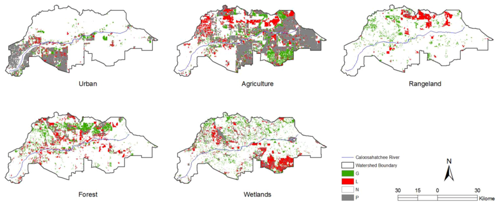
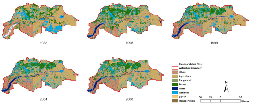
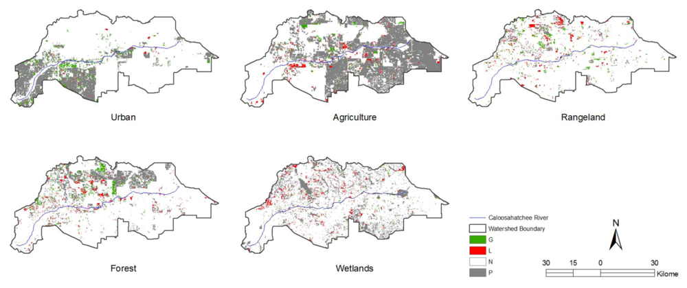
From Figure 2, there were more wetlands in the southeastern portions of the watershed in 1988. However, these may have been converted to agriculture soon thereafter based on the maps from subsequent years. This is not unusual, as there has been extensive drainage of wetlands in the area to make room for agriculture and other land uses [34]. 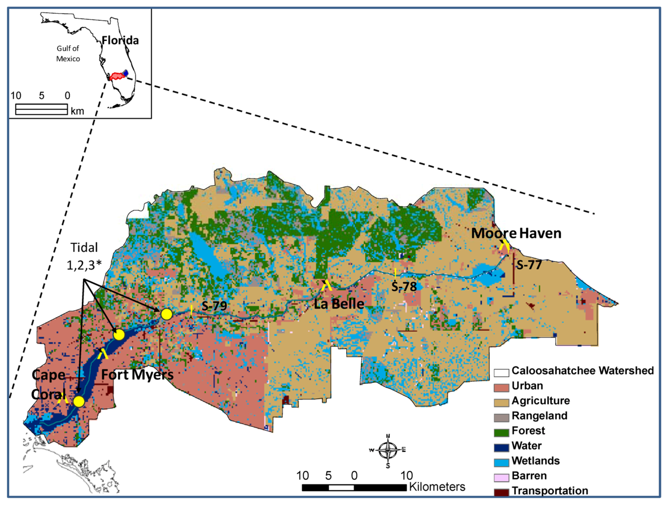Forests were more prevalent in 1995 than in the other years, based on Table 2, and particularly in the northern part of the watershed (Figure 2). Urban areas occurred primarily in the tidal portion of the watershed (downstream of S-79, Figure 1); these areas have experienced some increases throughout the study period, based on Table 2. Transportation was not mapped as extensively in other years as it was in 1995, based on further assessment of the spatial data; in particular, transportation was only mapped for the tidal portion in the 1988 land use, and while more extensive in the other years, the mapping was not as extensive for the tidal portion. For these reasons, changes involving transportation land use were excluded from further analyses. Overall, agriculture has been the dominant land use across the years, occupying >40% of the watershed area, with urban, wetlands and forest land uses being the next largest, and ranging between 16–21%, 15–17% and 13–18% of the watershed area, respectively.

Figure 2. Land-use in the Caloosahatchee River watershed during various periods, as determined from analyses of existing data.

Figure 2. Land-use in the Caloosahatchee River watershed during various periods, as determined from analyses of existing data.

Table 2. Land-use distribution (% of analyzed area, 1988–2008) in the study watershed.

Land Use	1988	1995	1999	2004	2008
Agriculture	46.3	42.0	44.2	43.5	43.3
Urban	17.8	16.3	18.1	19.4	20.3
Wetlands	16.0	15.7	16.4	16.7	14.9
Forest	13.3	18.1	14.0	13.5	14.1
Rangeland	5.5	5.5	6.0	5.5	5.9
Barren	0.7	1.0	0.6	0.6	0.5
Transportation*	0.4	1.4	0.7	0.7	0.9

*Transportation and utilities land use was not mapped as extensively in other years, as it was in 1995, thus values may not necessarily reflect change in the land use.

Table 2. Land-use distribution (% of analyzed area, 1988–2008) in the study watershed.

Land Use	1988	1995	1999	2004	2008
Agriculture	46.3	42.0	44.2	43.5	43.3
Urban	17.8	16.3	18.1	19.4	20.3
Wetlands	16.0	15.7	16.4	16.7	14.9
Forest	13.3	18.1	14.0	13.5	14.1
Rangeland	5.5	5.5	6.0	5.5	5.9
Barren	0.7	1.0	0.6	0.6	0.5
Transportation*	0.4	1.4	0.7	0.7	0.9

*Transportation and utilities land use was not mapped as extensively in other years, as it was in 1995, thus values may not necessarily reflect change in the land use.

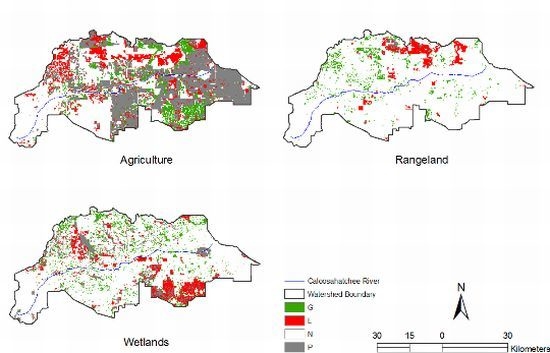
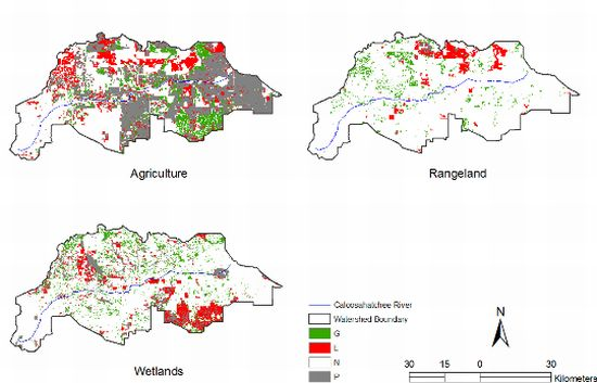
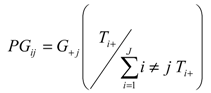
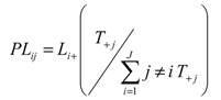
Table 3 shows gains, losses, net changes and persistence of land uses in the Caloosahatchee River Watershed based on analyses of existing data. Figure 3 and Figure 4 show gains (G), losses (L) and persistence (P) of the major land uses in the watershed between 1988 and 1999 (Figure 3) and between 1999 and 2008 (Figure 4). From Table 3, agriculture experienced the highest gains during the period 1988–2008 (10%), with these gains mostly occurring between 1988 and 1999. Similarly, agriculture experienced the largest losses (12.7%), with the largest being in the 1988–1999 period. Despite these changes, the overall net change for agriculture during 1988-2008 was relatively low (2.7%), indicating that the gains balanced the losses. Interestingly, urban areas experienced a corresponding gain (2.7%) during the same time period, based on Table 3.

Table 3. Gains, losses, net changes and persistence of land uses in the Caloosahatchee River Watershed, based on existing data.

	Period
	88–95	95–99	99–04	04–08	88–99	99–08	88–08
Gains
Urban	2.8	3.2	1.6	1.3	3.2	2.6	4.8
Agriculture	8.1	5.9	1.1	1.0	10.1	1.7	10.0
Rangeland	4.6	3.8	0.9	1.8	5.3	2.2	5.5
Forest	11.1	3.6	0.9	2.0	8.3	2.5	8.5
Wetlands	8.1	4.7	0.8	0.5	8.5	0.9	7.3
Barren	0.7	0.3	0.2	0.1	0.4	0.2	0.4
Losses
Urban	4.1	1.5	0.2	0.3	2.7	0.4	2.1
Agriculture	11.9	4.1	1.6	1.1	12.2	2.3	12.7
Rangeland	4.5	3.5	1.4	1.4	4.8	2.3	5.1
Forest	6.1	8.0	1.3	1.4	7.6	2.3	7.6
Wetlands	8.5	3.8	0.6	2.4	8.1	2.7	8.5
Barren	0.4	0.6	0.2	0.1	0.4	0.2	0.5
Net Change
Urban	−1.3	1.7	1.3	0.9	0.5	2.3	2.7
Agriculture	− 3.7	1.8	−0.5	−0.1	−2.1	−0.6	− 2.7
Rangeland	0.1	0.3	−0.5	0.5	0.5	−0.1	0.4
Forest	5.0	− 4.4	−0.4	0.6	0.7	0.2	0.9
Wetlands	−0.3	0.8	0.1	−1.9	0.4	−1.8	−1.2
Barren	0.3	−0.3	0.0	0.0	0.0	0.0	−0.1
Normalized Persistence
Urban	0.77	0.91	0.99	0.98	0.85	0.98	0.88
Agriculture	0.75	0.90	0.96	0.98	0.74	0.95	0.73
Rangeland	0.19	0.38	0.77	0.75	0.13	0.62	0.07
Forest	0.55	0.57	0.91	0.90	0.44	0.84	0.43
Wetlands	0.48	0.75	0.96	0.86	0.50	0.84	0.48
Barren	0.42	0.32	0.74	0.76	0.30	0.64	0.20

Table 3. Gains, losses, net changes and persistence of land uses in the Caloosahatchee River Watershed, based on existing data.

	Period
	88–95	95–99	99–04	04–08	88–99	99–08	88–08
Gains
Urban	2.8	3.2	1.6	1.3	3.2	2.6	4.8
Agriculture	8.1	5.9	1.1	1.0	10.1	1.7	10.0
Rangeland	4.6	3.8	0.9	1.8	5.3	2.2	5.5
Forest	11.1	3.6	0.9	2.0	8.3	2.5	8.5
Wetlands	8.1	4.7	0.8	0.5	8.5	0.9	7.3
Barren	0.7	0.3	0.2	0.1	0.4	0.2	0.4
Losses
Urban	4.1	1.5	0.2	0.3	2.7	0.4	2.1
Agriculture	11.9	4.1	1.6	1.1	12.2	2.3	12.7
Rangeland	4.5	3.5	1.4	1.4	4.8	2.3	5.1
Forest	6.1	8.0	1.3	1.4	7.6	2.3	7.6
Wetlands	8.5	3.8	0.6	2.4	8.1	2.7	8.5
Barren	0.4	0.6	0.2	0.1	0.4	0.2	0.5
Net Change
Urban	−1.3	1.7	1.3	0.9	0.5	2.3	2.7
Agriculture	− 3.7	1.8	−0.5	−0.1	−2.1	−0.6	− 2.7
Rangeland	0.1	0.3	−0.5	0.5	0.5	−0.1	0.4
Forest	5.0	− 4.4	−0.4	0.6	0.7	0.2	0.9
Wetlands	−0.3	0.8	0.1	−1.9	0.4	−1.8	−1.2
Barren	0.3	−0.3	0.0	0.0	0.0	0.0	−0.1
Normalized Persistence
Urban	0.77	0.91	0.99	0.98	0.85	0.98	0.88
Agriculture	0.75	0.90	0.96	0.98	0.74	0.95	0.73
Rangeland	0.19	0.38	0.77	0.75	0.13	0.62	0.07
Forest	0.55	0.57	0.91	0.90	0.44	0.84	0.43
Wetlands	0.48	0.75	0.96	0.86	0.50	0.84	0.48
Barren	0.42	0.32	0.74	0.76	0.30	0.64	0.20

However, a look at Figure 3 and Figure 4 shows that these changes did not correspond with regard to spatial extent, rather that gains in agricultural lands came from primarily wetland areas, while urban and agriculture also experienced gains from other land uses in the watershed. Forests experienced gains of 5% in 1988–1995 and an almost corresponding loss (4.4%) in the subsequent time period. Overall, forests did not experience large changes beyond 1999 and maintained high levels of persistence (≈0.9 or 90% in 1999–2004 and 2004–2008). Barren land showed the lowest net change, as gains experienced in this land use almost always balanced the losses. Urban and agricultural lands experienced the highest level of persistence during the study period, with this being primarily in the period between 1999–2008 (0.95 and 0.98, respectively), suggesting that these land uses remained fairly stable relative to other land uses in the watershed during this period. Rangeland and barren land were the most dynamic land uses, with only 0.07 and 0.20 persistence, respectively. However, these land uses also occupied very small portions of the watershed area (≤6% and ≤1%).

Figure 3. Gains (G), losses (L) and persistence (P) of land uses in the Caloosahatchee River Watershed between 1988 and 1999 based on existing data. Areas not in the land use concerned are represented as “N”.

Figure 3. Gains (G), losses (L) and persistence (P) of land uses in the Caloosahatchee River Watershed between 1988 and 1999 based on existing data. Areas not in the land use concerned are represented as “N”.

Figure 4. Gains (G), losses (L) and persistence (P) of land uses in the Caloosahatchee River Watershed between 1999 and 2008, based on existing data. Areas not in the land use concerned are represented as “N”.

Figure 4. Gains (G), losses (L) and persistence (P) of land uses in the Caloosahatchee River Watershed between 1999 and 2008, based on existing data. Areas not in the land use concerned are represented as “N”.

Based on Figure 3, urban and agricultural lands both gained from wetlands, while forest land use gained from both rangeland and agricultural lands. This is consistent with information in Flaig and Capece [34], which shows increases in agriculture and decreases in wetlands and rangeland in the western portion of the watershed (between S79 and S78). However, this picture is not mirrored in east Caloosahatchee for which Flaig and Capece [34] showed increases in agriculture with corresponding decreases in range land and only very slight decreases in wetlands. Both agriculture and urban lands showed relatively higher levels of persistence during the period of 1988–1999 compared to the other land uses, consistent with the data shown in Table 3. In the period between 1999 and 2008, all land uses showed higher tendencies towards persistence in comparison to the preceding period, and in general. Wetlands, however, appeared to be more dynamic than the other land uses during this period. Urban areas were mainly located in the tidal portions of the watershed, while agriculture mostly occupied the upland portion of the watershed based on the two figures. This is also the current status of the watershed (Figure 1).

Table 4. Inter-category changes in the Caloosahatchee River Watershed in 1988–1999: Focus on gains.

	1999	1	2	3	4	5	6
		Urban	Agric	Range	Forest	Wetlands	Barren	Totals Time 1	Loss
1988
1	Urban	14.86	0.82	0.29	0.75	0.80	0.05	17.57	2.7
	PRij	14.86	3.34	0.99	1.69	1.78	0.07	22.7	7.9
	Dij	0.00	−2.52	−0.70	−0.94	−0.97	−0.01	−5.2	−5.2
	Bij	0.00	−0.76	−0.71	−0.56	−0.55	−0.20	−0.2	−0.7
2	Agric	1.49	34.63	2.62	3.81	4.12	0.19	46.86	12.2
		1.81	34.63	2.65	4.50	4.74	0.18	48.5	13.9
		−0.32	0.00	−0.03	−0.69	−0.63	0.01	−1.7	−1.7
		−0.18	0.00	−0.01	−0.15	−0.13	0.07	0.0	−0.1
3	Range	0.27	1.99	0.73	1.54	1.03	0.00	5.56	4.8
		0.21	1.06	0.73	0.53	0.56	0.02	3.1	2.4
		0.05	0.93	0.00	1.01	0.46	−0.02	2.4	2.4
		0.25	0.88	0.00	1.89	0.83	−0.83	0.8	1.0
4	Forest	0.90	2.78	1.37	5.83	2.47	0.05	13.40	7.6
		0.52	2.55	0.76	5.83	1.36	0.05	11.1	5.2
		0.38	0.23	0.61	0.00	1.11	0.00	2.3	2.3
		0.73	0.09	0.81	0.00	0.82	0.01	0.2	0.4
5	Wetlands	0.41	4.38	1.02	2.18	7.95	0.08	16.02	8.1
		0.62	3.05	0.90	1.54	7.95	0.06	14.1	6.2
		−0.21	1.34	0.12	0.64	0.00	0.02	1.9	1.9
		−0.34	0.44	0.13	0.42	0.00	0.30	0.1	0.3
6	Barren	0.12	0.13	0.03	0.04	0.08	0.18	0.59	0.4
		0.02	0.11	0.03	0.06	0.06	0.18	0.5	0.3
		0.10	0.02	0.00	−0.02	0.02	0.00	0.1	0.1
		4.30	0.19	−0.09	−0.27	0.42	0.00	0.3	0.4
Totals Time 2		18.04	44.74	6.06	14.15	16.45	0.56	100.0
Gain		3.18	10.11	5.33	8.31	8.50	0.39

Positive values of D_ij and B_ij indicate that the land use as it existed in time 2 tended to gain from the corresponding land use in time 1 [7,16]. For this table time 1= 1988, time 2 = 1999.

Table 4. Inter-category changes in the Caloosahatchee River Watershed in 1988–1999: Focus on gains.

	1999	1	2	3	4	5	6
		Urban	Agric	Range	Forest	Wetlands	Barren	Totals Time 1	Loss
1988
1	Urban	14.86	0.82	0.29	0.75	0.80	0.05	17.57	2.7
	PRij	14.86	3.34	0.99	1.69	1.78	0.07	22.7	7.9
	Dij	0.00	−2.52	−0.70	−0.94	−0.97	−0.01	−5.2	−5.2
	Bij	0.00	−0.76	−0.71	−0.56	−0.55	−0.20	−0.2	−0.7
2	Agric	1.49	34.63	2.62	3.81	4.12	0.19	46.86	12.2
		1.81	34.63	2.65	4.50	4.74	0.18	48.5	13.9
		−0.32	0.00	−0.03	−0.69	−0.63	0.01	−1.7	−1.7
		−0.18	0.00	−0.01	−0.15	−0.13	0.07	0.0	−0.1
3	Range	0.27	1.99	0.73	1.54	1.03	0.00	5.56	4.8
		0.21	1.06	0.73	0.53	0.56	0.02	3.1	2.4
		0.05	0.93	0.00	1.01	0.46	−0.02	2.4	2.4
		0.25	0.88	0.00	1.89	0.83	−0.83	0.8	1.0
4	Forest	0.90	2.78	1.37	5.83	2.47	0.05	13.40	7.6
		0.52	2.55	0.76	5.83	1.36	0.05	11.1	5.2
		0.38	0.23	0.61	0.00	1.11	0.00	2.3	2.3
		0.73	0.09	0.81	0.00	0.82	0.01	0.2	0.4
5	Wetlands	0.41	4.38	1.02	2.18	7.95	0.08	16.02	8.1
		0.62	3.05	0.90	1.54	7.95	0.06	14.1	6.2
		−0.21	1.34	0.12	0.64	0.00	0.02	1.9	1.9
		−0.34	0.44	0.13	0.42	0.00	0.30	0.1	0.3
6	Barren	0.12	0.13	0.03	0.04	0.08	0.18	0.59	0.4
		0.02	0.11	0.03	0.06	0.06	0.18	0.5	0.3
		0.10	0.02	0.00	−0.02	0.02	0.00	0.1	0.1
		4.30	0.19	−0.09	−0.27	0.42	0.00	0.3	0.4
Totals Time 2		18.04	44.74	6.06	14.15	16.45	0.56	100.0
Gain		3.18	10.11	5.33	8.31	8.50	0.39

Positive values of D_ij and B_ij indicate that the land use as it existed in time 2 tended to gain from the corresponding land use in time 1 [7,16]. For this table time 1= 1988, time 2 = 1999.

Table 5. Intercategory changes in the Caloosahatchee River Watershed in 1988–1999: Focus on losses.

	1999	1	2	3	4	5	6	Totals Time 1
		Urban	Agric	Range	Forest	Wetlands	Barren		Loss
1988
1	Urban	14.86	0.82	0.29	0.75	0.80	0.05	17.57	2.72
	PRij	14.86	1.48	0.20	0.47	0.55	0.02	17.57
	Dij	0.00	−0.67	0.09	0.28	0.26	0.04	0.00
	Bij	0.00	−0.45	0.46	0.60	0.48	1.91	0.00
2	Agric	1.49	34.63	2.62	3.81	4.12	0.19	46.86	12.2
		3.99	34.63	1.34	3.13	3.64	0.12	46.86
		−2.50	0.00	1.28	0.68	0.48	0.07	0.00
		−0.63	0.00	0.95	0.22	0.13	0.56	0.00
3	Range	0.27	1.99	0.73	1.54	1.03	0.00	5.56	4.8
		0.93	2.30	0.73	0.73	0.85	0.03	5.56
		−0.66	−0.31	0.00	0.81	0.18	−0.03	0.00
		−0.71	−0.13	0.00	1.12	0.21	−0.87	0.00
4	Forest	0.90	2.78	1.37	5.83	2.47	0.05	13.40	7.6
		1.59	3.94	0.53	5.83	1.45	0.05	13.40
		−0.69	−1.16	0.83	0.00	1.02	0.00	0.00
		−0.44	−0.29	1.56	0.00	0.70	0.06	0.00
5	Wetlands	0.41	4.38	1.02	2.18	7.95	0.08	16.02	8.1
		1.74	4.32	0.59	1.37	7.95	0.05	16.02
		−1.34	0.06	0.44	0.81	0.00	0.03	0.00
		−0.77	0.01	0.75	0.59	0.00	0.48	0.00
6	Barren	0.12	0.13	0.03	0.04	0.08	0.18	0.59	0.4
		0.07	0.18	0.02	0.06	0.07	0.18	0.59
		0.05	−0.05	0.01	−0.02	0.02	0.00	0.00
		0.62	−0.28	0.20	−0.29	0.25	0.00	0.00
Totals Time 2		18.04	44.74	6.06	14.15	16.45	0.56	100.0
		23.18	46.86	3.42	11.59	14.50	0.45
		−5.14	−2.13	2.65	2.56	1.95	0.11
		−0.22	−0.05	0.77	0.22	0.13	0.24

Positive values of D_ij and B_ij indicate that the land use as it existed in time 1 tended to lose to the corresponding land use in time 2 [7,16]. For this table time 1= 1988, time 2 = 1999.

Table 5. Intercategory changes in the Caloosahatchee River Watershed in 1988–1999: Focus on losses.

	1999	1	2	3	4	5	6	Totals Time 1
		Urban	Agric	Range	Forest	Wetlands	Barren		Loss
1988
1	Urban	14.86	0.82	0.29	0.75	0.80	0.05	17.57	2.72
	PRij	14.86	1.48	0.20	0.47	0.55	0.02	17.57
	Dij	0.00	−0.67	0.09	0.28	0.26	0.04	0.00
	Bij	0.00	−0.45	0.46	0.60	0.48	1.91	0.00
2	Agric	1.49	34.63	2.62	3.81	4.12	0.19	46.86	12.2
		3.99	34.63	1.34	3.13	3.64	0.12	46.86
		−2.50	0.00	1.28	0.68	0.48	0.07	0.00
		−0.63	0.00	0.95	0.22	0.13	0.56	0.00
3	Range	0.27	1.99	0.73	1.54	1.03	0.00	5.56	4.8
		0.93	2.30	0.73	0.73	0.85	0.03	5.56
		−0.66	−0.31	0.00	0.81	0.18	−0.03	0.00
		−0.71	−0.13	0.00	1.12	0.21	−0.87	0.00
4	Forest	0.90	2.78	1.37	5.83	2.47	0.05	13.40	7.6
		1.59	3.94	0.53	5.83	1.45	0.05	13.40
		−0.69	−1.16	0.83	0.00	1.02	0.00	0.00
		−0.44	−0.29	1.56	0.00	0.70	0.06	0.00
5	Wetlands	0.41	4.38	1.02	2.18	7.95	0.08	16.02	8.1
		1.74	4.32	0.59	1.37	7.95	0.05	16.02
		−1.34	0.06	0.44	0.81	0.00	0.03	0.00
		−0.77	0.01	0.75	0.59	0.00	0.48	0.00
6	Barren	0.12	0.13	0.03	0.04	0.08	0.18	0.59	0.4
		0.07	0.18	0.02	0.06	0.07	0.18	0.59
		0.05	−0.05	0.01	−0.02	0.02	0.00	0.00
		0.62	−0.28	0.20	−0.29	0.25	0.00	0.00
Totals Time 2		18.04	44.74	6.06	14.15	16.45	0.56	100.0
		23.18	46.86	3.42	11.59	14.50	0.45
		−5.14	−2.13	2.65	2.56	1.95	0.11
		−0.22	−0.05	0.77	0.22	0.13	0.24

Positive values of D_ij and B_ij indicate that the land use as it existed in time 1 tended to lose to the corresponding land use in time 2 [7,16]. For this table time 1= 1988, time 2 = 1999.

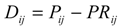
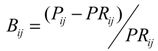
Table 4 and Table 5 show inter-category changes in the Caloosahatchee River watershed with a focus on gains (Table 4) and losses (Table 5). Based on these tables, forests and wetlands had the tendency to gain from rangeland (B_ij = 1.89, 0.83, respectively; Table 4), while rangeland showed a corresponding tendency to lose to forests and wetlands (B_ij = 1.12, 0.21, respectively; Table 5). Rangeland and wetlands showed a tendency to gain from forests (B_ij = 0.81, 0.82, respectively), while forest showed a corresponding tendency to lose to the two land uses (B_ij = 1.56, 0.70, respectively). Agriculture, rangeland, forest and barren lands showed the tendency to gain from wetlands (B_ij = 0.44, 0.13, 0.42 and 0.30, respectively), while wetlands showed a corresponding tendency to lose to these land uses (B_ij = 0.01, 0.75, 0.59 and 0.48, respectively), even though the signal for agriculture was very weak.

Both urban and wetlands showed the tendency to gain from barren lands (B_ij = 4.30, 0.42, respectively), and the corresponding tendency for barren lands to lose to urban and wetlands was seen in Table 5 (B_ij = 0.52, 0.25, respectively). While both urban and agriculture showed a tendency to gain from rangelands based on Table 4 (B_ij = 0.25, 0.88), a corresponding tendency for rangelands to lose to these land uses was not seen in Table 5. Similarly, results from the gains- and loss-based analyses did not correspond with respect to forests and urban lands. Thus, the associated results were disregarded to avoid misinterpretation, consistent with information in [16].

Similarly, for the period 1999–2008, barren lands showed the tendency to gain from agriculture (B_ij = 0.22), while agriculture showed a corresponding tendency to lose to barren lands (B_ij = 3.36). While all land uses showed the tendency to gain from rangelands (B_ij ranging from 1.12 for urban to 4.62 for forest), rangeland only showed a corresponding tendency to lose to forests and barren land (B_ij = 1.82, 1.50, respectively) based on the loss matrix. Urban, rangeland and wetlands showed the tendency to gain from forest (B_ij = 0.50, 1.70, 1.32, respectively), while forest only showed a tendency to lose to urban and rangelands ((B_ij = 0.24, 4.67, respectively). Rangelands and forests had the tendency to gain from wetlands (B_ij = 0.65, 1.27, respectively), while wetlands showed the tendency to lose to both land uses (B_ij = 2.45, 1.41, respectively). Corresponding tendencies were also found between urban and rangelands and barren lands (B_ij = 3.14, 3.70, respectively, for gains; B_ij = 0.80, 4.18, respectively, for losses).

In general, barren lands tended to convert to urban, rangeland and, to some extent, wetlands, based on matrices for 1988–2008. Additionally, rangelands tended to convert to forests and wetlands, forests to rangeland and wetlands and wetlands to rangeland and forest, based on the analyses. As with the periods of 1988–1999 and 1999–2008, there were tendencies for gains that were not mirrored in the loss matrix and vice versa. These were left out to avoid misinterpretation.

3.2. Census Data

Figure 5 shows populations in the various urban centers in the watershed along with the proportions of urban and agricultural land uses in the watershed. Based on Figure 5, population increased dramatically in Cape Coral between 1983 and 2007, peaked shortly thereafter and then started on a downward trend. A similar trend was seen in Fort Myers, although the increases were not as dramatic as those seen in Cape Coral. While urban areas increased somewhat during the same time period, the increase was not very large. In fact, the trend in urban land use somewhat mirrored that of Fort Myers. The cities of Fort Myers and Cape Coral make up the bulk of the urban areas in the tidal portion of the watershed, which is almost entirely urban. That the combined population for this area has shown such a great increase (≈130%) over the past 25 years or so while the area in urban land has increased only minimally (2.7%) during the same time period suggests that any new urban developments were likely cut out from areas already designated as urban. This is not uncommon, especially for older cities in which new development consists of demolishing older buildings and putting up new, modern, higher-occupancy buildings and/or converting existing land covers from lower or medium density to medium and/or higher density developments. As seen from the land use data analyses, agricultural land uses experienced a slightly downward trend during the study period. Based on Figure 5, the cities of LaBelle and Moore Haven did not experience any substantial changes in population during this time period. These two cities are the major urban centers in the upland (agricultural) portion of the watershed. From the analyses, this area has remained fairly stable during the past 25 years or so, as far as land use is concerned.

Figure 5. Populations in the various urban centers in the watershed along with proportions of urban and agricultural land uses in the watershed.

Figure 5. Populations in the various urban centers in the watershed along with proportions of urban and agricultural land uses in the watershed.

3.3. Hydrologic Trends

3.3.1. Trend Analyses

Figure 6 shows time series charts for annual maximum and mean flows at the three stations in the Calooshatchee River Watershed. Table 6 shows test statistics for the same time series at the stations. Based on Figure 6, annual maximum flows at all stations and annual mean flows at S-78 and S-79 showed upward trends over the long-term. A downward trend was observed for mean flows at S-77. Based on Table 6, however, these trends were only significant for the annual maximum time series at S-79 (p-value < 0.05). This time series was further analyzed to detect points at which changes occurred.

Figure 6. Annual maximum and mean flow time series at the three stations in the Calooshatchee River Watershed.

Figure 6. Annual maximum and mean flow time series at the three stations in the Calooshatchee River Watershed.

Table 6. Results from trend analyses of annual maximum and mean time series for Caloosahatchee.

Statistic	S-77		S-78		S-79
	Max	Mean	Max	Mean	Max	Mean
Spearman’s Rho	0.1640	−0.1590	0.2194	0.2625	0.3192	0.2025
p0.05	0.1955	0.2096	0.2358	0.1537	0.0370*	0.1928
Kendalls Tau	0.0879	−0.0863	0.1398	0.1871	0.2317	0.1561
p0.05	0.3051	0.3134	0.2693	0.1392	0.0287*	0.1400
Regression Slope	0.4772		1.1309		2.8563
Slope/RMSE	0.0086		0,0184		0.0220

Table 6. Results from trend analyses of annual maximum and mean time series for Caloosahatchee.

Statistic	S-77		S-78		S-79
	Max	Mean	Max	Mean	Max	Mean
Spearman’s Rho	0.1640	−0.1590	0.2194	0.2625	0.3192	0.2025
p0.05	0.1955	0.2096	0.2358	0.1537	0.0370*	0.1928
Kendalls Tau	0.0879	−0.0863	0.1398	0.1871	0.2317	0.1561
p0.05	0.3051	0.3134	0.2693	0.1392	0.0287*	0.1400
Regression Slope	0.4772		1.1309		2.8563
Slope/RMSE	0.0086		0,0184		0.0220

3.3.2. Change Detection

Results from CUSUM analyses showed a downward trend until 1978 (Figure 7(a,b)). Flows remained more or less constant until 1980, then experienced a general increase until 1987, followed by a decrease up to 1991. The flows showed some fluctuations between 1991 and 2000, after which there was a more or less steady increase up to 2009. Comparison over change periods as identified using CUSUM analyses are shown in Figure 7(c). Based on the Wilcoxon/Kruskal-Wallis and Median tests, there were significant differences in annual maximum flows between the change periods (p_0.05 = 0.0061, 0.0017, respectively). Further analyses using the t-test showed that flows in the period 1988–1991 were significantly different from those in 2001–2009 (p_0.05 = 0.0052), but neither of the flows were significantly different from flows in 1992–2000. Results also showed that the flows in 1967–1980 and 1988–1991 were both significantly different from those in 1981-1987 (p_0.05 = 0.0316, 0.0147, respectively). Flows in 1967–1980 were also significantly different from those in 2001–2009 (p_0.05 = 0.0073). Comparison over the land use study periods (Figure 7(d)) did not show significant differences among the periods in a general sense based on the Wilcoxon/Kruskal-Wallis and Median tests (p_0.05 = 0.1026, 0.0552, respectively), although results of the median test could be considered significant at α = 0.1. Further analyses using the t-test showed a borderline significant difference between annual maximum flows in 1967–1980 and those in 1981–1987 (p_0.05 = 0.0467); no other significant differences were observed.

Figure 7. Results of analyses to detect points of change in annual maximum time series at S-79. (a) Comparison to long-term median. (b) CUSUM values. (c) Comparison of flows during various periods identified in (b). (d) Comparison of flows during the land use study periods.

Figure 7. Results of analyses to detect points of change in annual maximum time series at S-79. (a) Comparison to long-term median. (b) CUSUM values. (c) Comparison of flows during various periods identified in (b). (d) Comparison of flows during the land use study periods.

3.3.3. Climate Trends

Preliminary analyses showed that only the maximum and mean time series data showed independence and only the maximum time series were normal or near-normal. Thus, further tests were only carried out on these two time series. No appreciable trends were observed in climate data based on Spearman’s Rho and the Mann-Kendall test (p-values > 0.05), as well as from the regression analyses, consistent with information in [34]. Thus, trends and differences detected in flow time series could be attributed to landscape and/or management changes, rather than climate trends.

3.4. Water Quality Trends

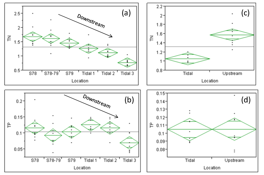
From Figure 8(a), total nitrogen (TN) concentrations decreased coming from the upland to the tidal portion of the watershed, with nitrogen concentrations being above the global mean for the watershed (solid horizontal line) in the upland portion and below the mean in the tidal portion of the watershed. Comparison test showed that TN concentrations were significantly different among the various locations (p_0.05 = 0.0001). In contrast, phosphorus concentrations (Figure 8(b)) were scattered among the locations, with no clear trend being observed. In the upland portion of the watershed, total phosphorus (TP) concentrations were higher above S-78, this possibly being reflective of discharges from Lake Okeechobee, and dropped between S78-79. However, concentrations increased again at S-79, possibly reflecting contributions from agricultural lands. Mean concentrations in the tidal portions of the watershed (Tidal 1 and Tidal 2) were higher than those at S-79 and between S-78 and S-79, but were close to the mean concentration at S-78. This increase in TP concentrations in the tidal portions of the watershed is possibly indicative of contributions from the urban lands surrounding that area. Concentrations at Tidal 3 were much lower than those from all the other sections of the watershed, possibly due to a dilution effect and/or from influx of sea water and storm surges. TP concentrations at Tidal 1 and Tidal 2 were comparable to those at S-78, which are reflective of inflows from Lake Okeechobee.

Figure 8. (a) Total N concentrations (mg/L) along the Caloosahatchee River. (b) Total P concentrations (mg/L) along the Caloosahatchee River. (c) Comparisons between upstream and tidal reaches for Total N. (d) Comparisons between upstream and tidal reaches for Total P.

Figure 8. (a) Total N concentrations (mg/L) along the Caloosahatchee River. (b) Total P concentrations (mg/L) along the Caloosahatchee River. (c) Comparisons between upstream and tidal reaches for Total N. (d) Comparisons between upstream and tidal reaches for Total P.

Comparison test for TP also showed significant differences among the various locations (p_0.05 = 0.0133). Comparing the averages for the upland and tidal portions of the watershed (Figure 8(c)) for TN, concentrations in the upland areas of the watershed were significantly higher (p_0.05 = 0.0003) than those in the tidal portions of the watershed. For TP (Figure 8(d)), there were no significant differences between average upland and tidal concentrations (p_0.05 = 0.8946). These findings were confirmed through an analysis of more detailed data at S-79 and at Tidal 1, in which TN differences were found to be significant (p_0.05 = 0.0002), while those for TP were not significant (p_0.05 = 0.0617). An analysis of more detailed data showed a significant downward trend with time in TN (Kendall’s Tau = −4074; p_0.05 = 0.0023) at S-79. TN at Tidal 1 also exhibited a significant downward trend (Kendall’s Tau = −0.2934; p_0.05 = 0.0318) over the years, although not as strongly as at S-79. At S-79, TP also exhibited a significant downward trend over time (Kendall’s Tau = −0.3757; p_0.05 = 0.0050) based on analyses of detailed data. TP trends were, however, not significant at Tidal 1.

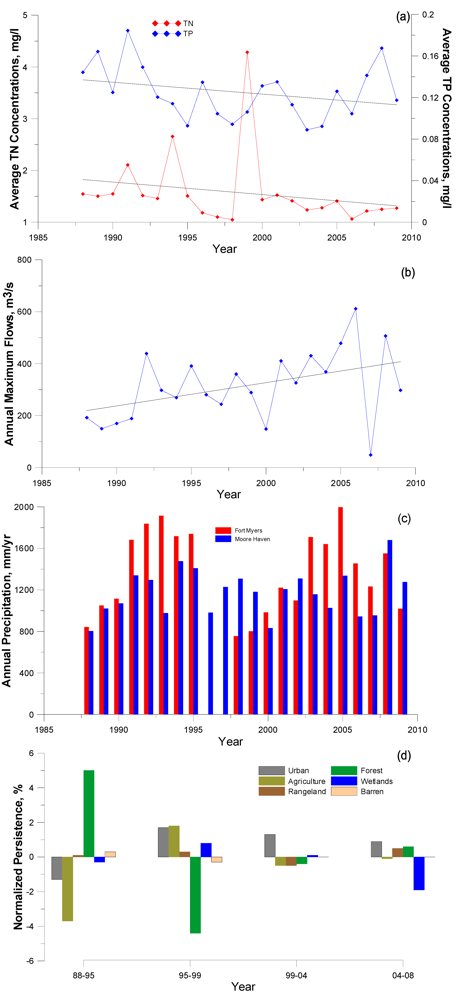
Figure 9. (a) mean daily total nitrogen (TN) and total phosphorus (TP) concentrations. (b) daily maximum flows. (c) annual precipitation at Fort Myers and Moore Haven. (d) net changes in land use (%). Flow and nutrient values are from/for S-79.

Figure 9. (a) mean daily total nitrogen (TN) and total phosphorus (TP) concentrations. (b) daily maximum flows. (c) annual precipitation at Fort Myers and Moore Haven. (d) net changes in land use (%). Flow and nutrient values are from/for S-79.

Based on Figure 9(a,b), there was a general decrease in TN and TP concentrations between 1988 and 2009 and a steady increase in maximum daily flows at S-79, consistent with previous results. The general decrease in concentrations might be attributable to a dilution effect resulting from the general increase in flows, or might be reflective of a change in management in the watershed. A look at climate data Figure 9(c) showed that precipitation followed a normal cyclic pattern with periods of highs and lows, typical of precipitation in many areas. As seen previously, the major changes in land use occurred in the period between 1988 and 1999, with forests experiencing the largest gain in 1988–1995 and a subsequent loss in 1995–1999. Agriculture and urban areas experienced a corresponding loss in 1988–1995 and subsequent gains in 1995–1999. Wetlands experienced an appreciable decrease in 2004–2008, a loss which was spread out among the other land uses.

3.5. General Discussion

Based on the analysis of land use data, agriculture and urban land uses experienced the highest levels of persistence, with the land uses experiencing a net decrease and a net increase of 2.7%, respectively. More detailed assessments, however, showed that gains in urban areas did not occur in the same spatial locations as did losses in agricultural lands, and thus, gains in urban areas were not a result of losses in agriculture. While the net changes observed in agricultural and urban lands are relatively low during the study period, current coverage is reflective of tremendous changes that have occurred historically, following channelization of the main channel and construction of flow regulating structures [22]. These land uses combined occupied less than 2% of the watershed area in the late 1950s, with the watershed being primarily in forest and wetlands at that time [34]. Additionally, results from analysis of census data suggest that a substantial change might have occurred in land cover within already existing urban land use areas during the study period. While forests and wetlands exhibited relatively high levels of persistence in 1999–2008 (84%), their overall persistence over the land use study period was low (43% and 48%, respectively). This lack of persistence was also reflected in the developed maps. Wetlands are difficult to map due to their highly dynamic nature [35,36], and their classification is often reflective of the existing management and/or hydrologic regime [36]. Thus, while major changes in wetlands can be discerned from the analyses, transitions between wetlands, and (particularly) forests and rangelands, may be more reflective of the status at the time of classification, rather than of true land use changes.

Significant trends in time series data in the period of 1988–2008 were mainly observed at S-79. These included increases in maximum daily flows at S-79, as well as decreases in TN and TP concentrations. While trends were observed in some of the other time series that were analyzed, they were not significant. Based on existing literature, however, changes in daily flows do occur over the course of a year with great variations between seasons [22,34]. 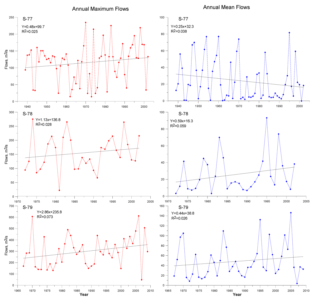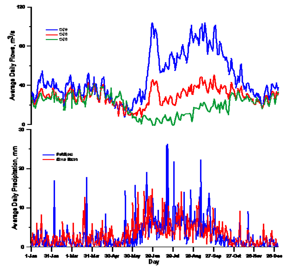This is reflected in Figure 10, which shows average daily flows at the three stations in the watershed during the period of 1988–2002 (2002 was used as the cutoff for comparison purposes, as two of the stations only had data through 2002). During the summer months (June–October), flow through S-79 often exceeded the recommended 70 m³/s documented in [34], which has implications on the ecological well-being of the Caloosahatchee estuary. While flows during November to May did not differ much among the stations, flows were much higher at S-79 than at the other two stations and were also higher at S-78 than at S-77. The latter reflects primarily discharges from Lake Okeechobee, while the former two reflect primarily contributions from the watershed, consistent with information in [37]. There were no appreciable trends in precipitation, based on the analyses of long-term data. In addition, changes in hydrology and water quality were not necessarily reflective of changes in land use; rather, these changes were thought to be reflective of changes in the management of the stream channel to meet ecological needs. Further, since no appreciable changes occurred in agricultural land use during the land use study period, decreases in nutrient concentrations could also be attributable to changes in management within existing agricultural land use. The data did, however, show somewhat higher TP concentrations in the tidal portion of the watershed than in the mid (agricultural) section of the watershed, suggesting substantial contributions from urban areas. This is in line with census data, which showed a rapidly increasing urban population in an area that did not exhibit corresponding spatial expansion.

Figure 10. Average daily flows and precipitation (secondary Y-axis) at the Caloosahatchee stations during the period of 1988–2002.

Figure 10. Average daily flows and precipitation (secondary Y-axis) at the Caloosahatchee stations during the period of 1988–2002.

Overall, results provided useful information and insights into the extent, nature of and possible impacts of land use and related changes that have occurred in the watershed in the recent past, all of which can be used for watershed decision making. For example, results suggest that there have been localized changes within urban land uses and that these changes are potentially impacting estuarine water quality, thus pointing to the need for a more in-depth assessment of this land use and, similarly, for agriculture. In this regard, the information obtained can also be used to guide the development of conservation measures and/or land use development policies. Results also show that stream flow patterns along the main channel are not reflective of watershed dynamics, thus pointing to the need to monitor tributary channels more extensively in order to better characterize watershed responses for future watershed decision making. Further assessments using automated modeling techniques, such as those described in [38,39,40], would allow more detailed evaluation and would be especially useful in detecting additional historical patterns that are otherwise not discernible. The accuracy of modeling techniques, however, varies with the net change experienced and with the resolution of the data [40]. Thus, the results would also need to be interpreted in context, considering the historical perspective, and with a working knowledge of the watershed.

4. Conclusions

This study explored the use of a multi-layer approach in characterizing land use changes and their related impacts, with a view to determining its suitability for use in watershed decision making. The study used existing land use data, along with population, stream flow, climate and water quality data, for the analyses. In general, all datasets provided valuable insights into changes and dynamics occurring in the watershed. However, the datasets did not necessarily complement each other, and results could easily be confounding without an in-depth knowledge of the watershed from both a historical and current perspective. Nevertheless, the different information obtained from the datasets did serve to provide a broader perspective on watershed dynamics, making the methodology particularly useful in cases where existing land use data are limited and/or disparate. Further work using related modeling techniques would allow more detailed analyses and help provide further insights into watershed dynamics. With respect to decision making, the approach and associated results provide the information necessary to allow watershed decision makers to discern current trends and their impacts, as well as to anticipate possible future scenarios based on existing trends. This would, in turn, aid in developing knowledge-based strategies and practices for environmental protection to prevent or minimize such impacts consistent with [5]. While our results are site-specific, the approaches and methodologies used are applicable to other watersheds beyond the study site.