Relationship between Industrial Water Use and Economic Growth in China: Insights from an Environmental Kuznets Curve

Abstract

Global inequity and the unbalance of water resources has been a critical issue for many years; and the Chinese per capita water resources are only 1/4 of the global average. Meanwhile, as the Chinese economy is growing rapidly, the demand of Chinese industrial water use is also increasing. In this case, it is important to balance the relationship between economic growth and industrial water use. In this study, a reduction model is established for the northeastern, northern coastal, eastern coastal, southern coastal, middle Yellow River, middle Yangtze River, southwestern, and northwestern regions to verify the environmental Kuznets curve (EKC) for their respective industrial water use and provide theoretical support for decision making from an economic perspective. It adopts the per capita industrial water use and GDP of the eight economic zones from 2002 to 2014. The unit root test and co-integration test were adopted to analyze the stationarity of the data, and the triple reduction model was used for the fitting of variables. The relationship between per capita industrial water use and GDP showed an inverted U-shaped curve from 2002 to 2014 for China, as well as for the eastern coastal and middle Yangtze River regions, with the coordinates of the turning points being (9.8749, 4.6735), (10.3098, 5.4783), and (9.8184, 5.0622), respectively. The per capita GDP at the turning point of the inverted U-shaped curve is 18,000–30,000 Yuan (at constant prices from 2000). This study provides important thoughts and lessons for collaborative research into the relationship between industrial water consumption and economic development. The central government should focus on the central and western regions when creating policies for water resource management and technological development to improve their industrial water use efficiency.

1. Introduction

The insufficient and imbalanced water resources across the globe is an important problem facing the 21st century. The World Water Council [1] estimated that approximately 40% of the world population experiences water shortages, and the ratio is likely to reach 50% by 2025. As the most populous country, China accounts for 21% of the world population but possesses a measly 6% of global water resources, and its per capita water resources amount to merely 2048 m³ or 29% of the global average. The situation is severe. In the water use structure of China, agriculture accounts for the largest share, but the proportion is declining. By contrast, the proportion of industrial water use continues to grow. The National Bureau of Statistics [2] stated that the proportion of agricultural water use in China fell from 69% to 63% from 2000 to 2014, whereas that of industrial water use rose from 21% to 22%. The World Bank [3] estimates that before 2050, the agricultural water use rate will drop to roughly 50%, but the industrial water use rate will increase steadily. The Chinese government established goals for energy and water use intensity in the 12th Five-Year Plan, along with objectives for nationwide water use at the end of this five-year plan. Programs such as “Strengthening the Foundation through Industry” and “Intelligent Manufacturing in China” are advanced in the 13th Five-Year Plan, and Made in China 2025 is promulgated. China’s industrial economy will usher in rapid development, and industrial water demand is also projected to change. To create a well-rounded, moderately prosperous society by 2020, China will implement strict water resource management policies and control the consumption, as well as the consumption intensity, of water resources. Analyzing the relationship between industrial water use and economic development is considerably significant for removing the bottleneck problems related to the water resources of China. In this study, per capita industrial water use and GDP/GRP (hereinafter referred to as GDP) are used as indicators to investigate the EKC of China, in the northeastern, northern coastal, eastern coastal, southern coastal, middle Yellow River, middle Yangtze River, southwestern, and northwestern regions. Regional panel data from 2002 to 2014 were utilized for verifying and analyzing the EKC for industrial water use and economic development to provide a scientific reference for the concerted development of industrial water use and economic growth.

In 1955, Kuznets [4] advanced that the curve of income distribution will form an inverted U-shape with the course of economic development. That is, the gap of wealth will first increase and then decrease along with economic growth. This inverted U-shaped relationship is called the environmental Kuznets curve (EKC). Since 1992, scholars have conducted various EKC studies focusing on environmental pollution and energy. Panayotou et al. [5] verified the EKC relationship between environmental degradation and economic growth using forest logging rate and per capita income as indicators. Selden et al. [6] verified the EKC for air pollution with suspended particulate matters, SO₂, NO, CO, and per capita GDP as indicators. By studying the relationship between energy consumption and per capita GDP in 113 countries, Luzzati et al. [7] demonstrated that transnational EKC research requires more detailed discussion.

Foreign studies have been conducted on the EKC for water use, but few of them have focused on industrial water use. Consistent with the EKC hypothesis, Rock [8] suggested that both per capita water intake and water use follow an inverted U-shaped curve of development on the basis of cross-regional data for water intake and panel data for water use in the US. Katz [9] verified that the EKC has a certain limitation with regard to water policy making and planning; the curve cannot accurately represent the performance of an individual country. Gleick [10] indicated that no clear relevance exists between nationwide per capita water use and income, but the research did not adopt a rigorous method of statistical analysis. Hemati [11] studied the per capita industrial water use and income elasticity of 132 countries, verifying a bell-shaped relationship between the two.

In China, studies have been conducted to verify the EKC for industrial water use. Jia [12] studied the relationship between the per capita water use index and the GDP of OECD states and found that most OECD states follow the EKC for industrial water use; however, this study did not include a non-OECD state. Li Qiang et al. [13] studied the EKC for per capita industrial and domestic water use in China and confirmed that the EKC for per capita industrial water use exists, but the EKC for per capita agricultural and domestic water use is unavailable. Despite these important findings, the research could not provide a reliable reference for the industrial development of each region because of the considerable differences in regional economic and industrial development. Zhang Bingbing et al. [14] tested the industrial added value and water use for east, central, and west China and indicated that the relationship is represented by an inverted U-shaped curve for East China, an N-shaped curve for Central China, and an approximately progressive increase for China and West China. The research could not provide a prominent conclusion because the division of regions failed to feature the geographical characteristics and the per capita added industrial value. A portion of per capita GDP cannot represent the national economic level.

With regard to methodology, EKC is sensitive to data and statistical approaches. The smooth transition regression (STR) model was applied in the studies of Hemati [8], Bacon [15], and Teräsvirta [16]. The relatively common reduction model was employed by Cole [17], Katz [18], and Bhattarai [19]. The panel smooth transition regression (PSTR) model was adopted by Duarte [20] and Fouquau [21]. Katz [18] demonstrated that in EKC studies on pollution, the results were sensitive to the data selection and analytical method and that no method could make the per capita water recycled in all databases conform to an EKC. List et al. [22] analyzed the relationship between per capita emissions of SO₂ and NO and income in the US from 1929 to 1994 using the regression model and stated that it could verify the inverted U-shaped curve. Despite its prevalence, the inverted U-shaped relationship is not applicable to all data, and a statistical error may be generated if the model is used indiscriminately. With the quadratic polynomial fixed effect regression model and the PSTR model, Duarte et al. [20] verified the inverted U-shaped relationship between per capita water use and income of 65 countries from 1962 to 2008, but these models resulted in significantly different curve forms and estimated turning points as well as varying water use in different time periods and countries.

In general, the reduction model is applied frequently in EKC research. Katz [18] verified that the regression model is suitable for analyzing the relevance between economic growth and water use given the limitation of data collection. Grossman et al. [23] regressed environmental indexes to income or its square or cube; this simplified model can be used to emphasize the direct or indirect relationship with income. Moomaw et al. [24] demonstrated that the regression model cannot reflect the random factors in nature. Seldon et al. [25] also concluded that the regression model cannot account for other complicated influencing variables (e.g., politics and educational level). Rock [5] attempted to adopt a complex model, but many variable errors may be incurred because all relevant parameters should be covered.

In this study, per capita industrial water use and GDP are employed as indices to analyze the EKC for the industrial water use of the entire China along with the northeastern, northern coastal, eastern coastal, southern coastal, middle Yellow River, middle Yangtze River, southwestern, and northwestern regions. This study explores the relationship between the industrial water use and economic development of these regions on the basis of their unique development characteristics and development stages.

2. Materials and Methods

2.1. Method and Model

The reduction model proposed by Katz et al. [18] was employed in this study. This model can reflect the relevance between independent and dependent variables rather than the direct influence of the former on the latter. The method adopted is consistent with that of initial EKC research. The logarithm to the per capita GDP of China and each of the eight economic zones from 2002 to 2014 was derived as the independent variable, and the per capita industrial water use was obtained as the dependent variable. Logarithms of the independent and dependent variables were used because they can mitigate data fluctuation, remove the heteroscedasticity of the time series, and reduce the extremum, abnormal distribution, and heteroscedasticity of variables. This method is identical to that in the EKC research of Stern [25]. Consistent with the research of Katz [18], per capita data are employed because they can reflect the living standard directly, whereas nationwide industrial water use data is affected by population.

The reduction model was adopted, including the first power, square, and cube of the independent variable. The cubic model was used because per capita industrial water use does not decline after a turning point, and the model can display two turning points. The failed reflection of the original data trend and the reduced accuracy in the quadratic model could be avoided. List et al. [22] also adopted the cubic model.

The adopted reduction model was defined as follows:

$$\log {\mathrm{water}}_{it}={\beta }_0+a_i+{\beta }_1\times \log {\mathrm{GDP}}_{it}+{\beta }_2\times {\left(\log {\mathrm{GDP}}_{it}\right)}^2+{\beta }_3\times {\left(\log {\mathrm{GDP}}_{it}\right)}^3+e_{it}$$

(1)

where $\log {\mathrm{water}}_{it}$ represents the logarithm of per capita industrial water use in region i in year t; $\log {\mathrm{GDP}}_{it}$ is the logarithm of per capita GDP in region i in year t; ${\beta }_1,{\beta }_2,{\beta }_3$ represent the parameters to be identified in the model; $a_i$ is the correction factor of region i; and $e_{it}$ is the error term.

2.2. Samples and Data

The Development Research Center of the State Council [26] reported that the original division of China into eastern, central, and western regions cannot reasonably reflect regional characteristics because they cover a large area and population. The regional development strategy is now focused on the concerted development of all regions rather than only on coastal regions, and, thus, a detailed division of east, central, and west China is encouraged. In 2004, the Development Research Center of the State Council divided China into the northeastern, northern coastal, eastern coastal, southern coastal, middle Yellow River, middle Yangtze River, southwestern, and northwestern regions. Li Shantong et al. [27] suggested that the adjacent areas of each region possess similar natural conditions and resource structures.

To accurately represent the economic development characteristics of each region, analyze the regions with different features, and obtain results consistent with the actual economic development, this study divides China into eight regions. The northeastern region includes the provinces of Liaoning, Jilin, and Heilongjiang. The northern coastal region consists of Beijing Municipality, Tianjin Municipality, Hebei Province, and Shandong Province. The eastern coastal region comprises Shanghai Municipality, Jiangsu Province, and Zhejiang Province. The southern coastal region covers the provinces of Fujian, Guangdong, and Hainan. The middle Yellow River region includes Shanxi Province, the Inner Mongolia Autonomous Region, Henan Province, and Shaanxi Province. The middle Yangtze River region comprises provinces of Anhui, Jiangxi, Hubei, and Hunan. The southwestern region consists of Guangxi Zhuang Autonomous Region, Chongqing Municipality, Sichuan Province, Guizhou Province, and Yunnan Province. The northwestern region covers Tibet Autonomous Region, Gansu Province, Qinghai Province, Ningxia Hui Autonomous Region, and Xinjiang Uygur Autonomous Region. This division follows that of the eight economic zones of National Bureau of Statistics.

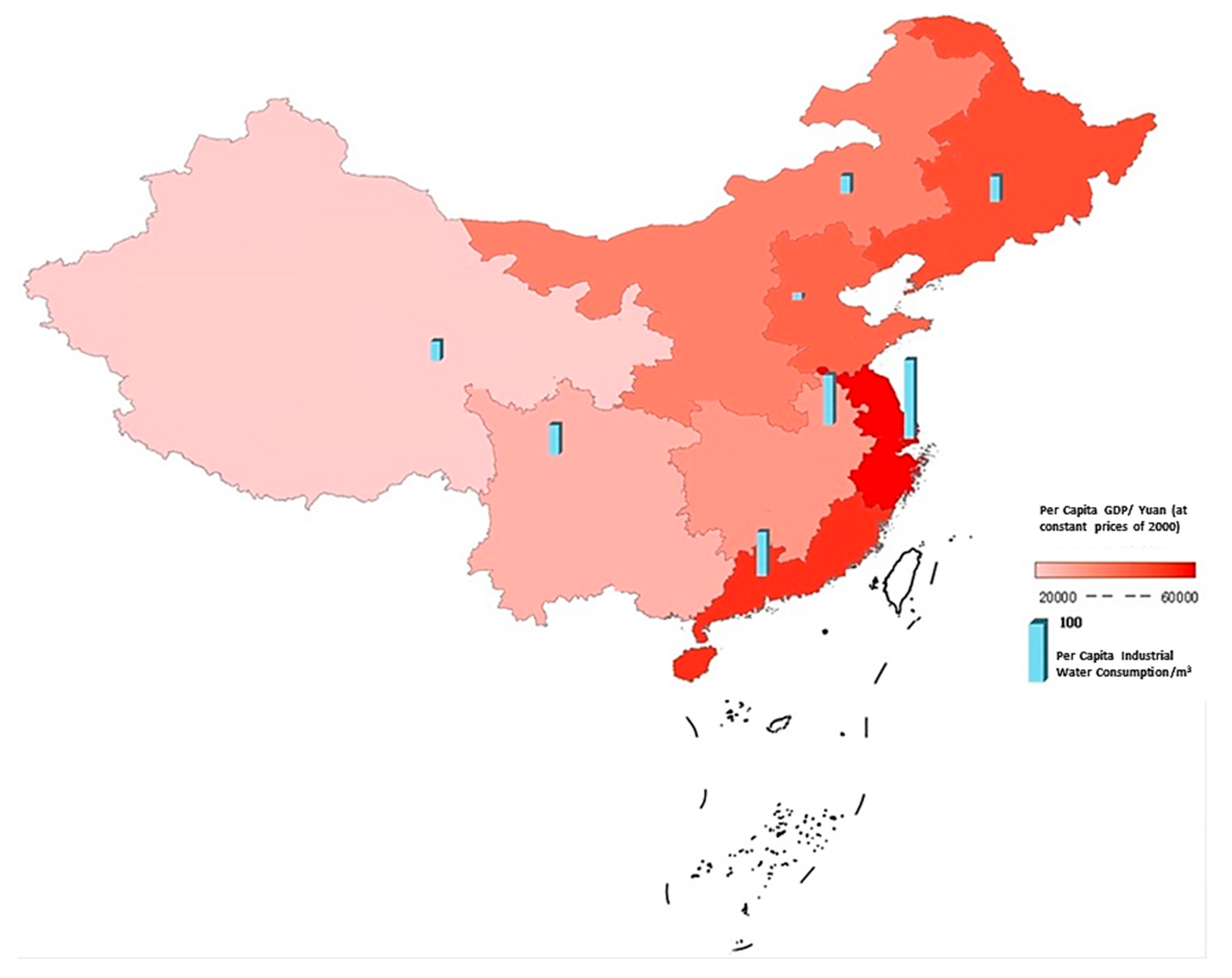
The relationship between per capita industrial water use and GDP of the eight regions from 2002 to 2014 was fitted and analyzed. The data included concerned industrial water use, population, and per capita GDP of each region. Data on total industrial water use were derived from the China Statistical Yearbook, although that of 2011 is missing. The mean value method was adopted; the mean value of two continuous years was taken for supplementation. Data on the per capita regional GDP for each province were provided by the National Bureau of Statistics. Current year prices of per capita GDP of each region were converted into constant prices based on 2000. The per capita regional GDP index, for which 100 was designated for 2000, was determined according to the per capita GDP index of the National Bureau of Statistics, for which 100 was designated for the previous year. Data on regional population were derived from the National Bureau of Statistics. Figure 1 illustrates the relationship between per capita industrial water use and GDP in 2014 for the eight economic zones. Most regions with higher GDP boast a greater per capita industrial water use.

3. Data Verification and Results

Two types of time series exist: the stationary and non-stationary time series. In the former, mean value, variance, and covariance do not change along with time displacement and the randomness on each time point is distributed according to certain probability. In the latter, mean value, variance, and covariance vary along with time placement.

In 1974, Granger et al. [28] stated that insufficient consideration had been given to the autocorrelation of residual error in many studies and that testing the significance of regression standards may be misguided by unstable macro data. In a non-stationary time series, the outstanding regression relationship between a variable and another random variable may result in spurious regression. A hypothesis and a unit root test should be made to investigate whether variables are integrated in the same order. On this basis, a co-integration test should be subsequently conducted. If a co-integration relationship exists in a group of non-stationary time series, then a linear combination exists in this group of data. Consequently, its mean value, variance, and covariance will no longer vary with time displacement. Under such circumstances, no spurious regression will be observed in the time series.

Data in this paper are in time series and its statistical law varies along with the change of time, thus becoming non-stationary. Therefore, a unit root test is conducted for each series through ADF (Augmented Dickey-Fuller test) before proceeding with variable regression. It reaches stationary series when the number of integration orders is identical. A co-integration test is then conducted on the series with a same number of integration orders to achieve a stationary or co-integration series and avoid spurious regression.

3.1. Unit Root Test

The unit root test of panel data can be conducted through various methods. The most commonly used methods include the ADF method proposed by Dickey et al. [29], the PP (Phillips&Perron) method proposed by Phillips et al., the ERS-DFGLS (Elliott, Rothenberg and Stock proposed Dickey-Fuller Test GLS Detrending (DFGLS)) method, and the Kwiatkowski–Philips–Schmidt–Shin (KPSS) method proposed by Elliott. The null hypothesis for the ADF, PP, and ERS methods are a non-stationary series. For the KPSS method, the null hypothesis is a stationary or trend stationary series. In this study, the most classic and common ADF method was adopted, and Eviews 8.0 was used to conduct the unit root test and the following co-integration test.

Given that three explaining variables exist, the number of integrated of order of all explained variables cannot be higher than that of any explaining variable. When the number of integrated of order of all explaining variables is greater than that of explained variables, two or more explaining variables whose number of integrated of order is greater than that of all the explained variables must exist. If the result of the unit root test indicates the non-same-order integration of variables, then the co-integration test and the following sequence analysis should not be conducted. In this study, data were verified at a confidence interval of 95% and 90%, but only the latter passed the verification. Nevertheless, the data passed the verification.

The result of the unit root test for the per capita GDP nationwide from 2002 to 2014 is shown in

Table 1. ADF (Augmented Dickey-Fuller test) test on per capita GDP index of China (2002–2014).

Unit Root Test Result	Critical Value under Significance Level			ADF Test Value	p Value
	1%	5%	10%
Original Sequence	−4.121990	−3.144920	−2.713751	−2.554599	(0.1280)
First-order Difference	−4.200056	−3.175352	−2.728985	−1.083218	(0.6812)
Second-order Difference	−4.297073	−3.212696	−2.747676	−3.015682	(0.0672)

. The test statistics of the original sequence based on the ADF method was −2.554599. This value was greater than the critical value under the 10% significance level, and the original sequence was non-stationary. The test statistics of first-order difference based on ADF was −1.083218, which remains greater than the critical value under the 10% significance level. After second-order difference, the test statistics was −3.015682, which is less than the 10% significance level. When the confidence coefficient is 90%, the time series after the second-order difference is stationary, indicating that the number of integration orders is two.

The unit root test was first conducted on $\log {\mathrm{water}}_{it}$, $\log {\mathrm{GDP}}_{it}$, ${\left(\log {\mathrm{GDP}}_{it}\right)}^2$, and ${\left(\log {\mathrm{GDP}}_{it}\right)}^3$ of China and its eight regions.

Given that the trend chart does not start from the original point and that the mode is non-linear, the intercept term, rather than the trend term, was included in the test. The maximum lag period of the difference term was defined as two by default. When the original data does not pass the unit root test, the first-order difference is conducted on the data for testing. If the data fails the test, the second-order difference test is conducted. The second-order difference test determines the number of integration orders of the corresponding data.

Table 2. Unit root test results of panel data.

Unit Root Test Result	$\mathbf{log}\mathbf{G}\mathbf{D}{\mathbf{P}}_{\mathit{i}\mathit{t}}$	${\left(\mathbf{log}\mathbf{G}\mathbf{D}{\mathbf{P}}_{\mathit{i}\mathit{t}}\right)}^2$	${\left(\mathbf{log}\mathbf{G}\mathbf{D}{\mathbf{P}}_{\mathit{i}\mathit{t}}\right)}^3$	$\mathbf{log}\mathbf{w}\mathbf{a}\mathbf{t}\mathbf{e}{\mathbf{r}}_{\mathit{i}\mathit{t}}$
China	−2.554599	−1.951466	−1.352739	−2.533588
Original sequence	−1.083218	−1.327039	−1.609779	−1.037902
First-order difference	−3.015682 *	−3.013465 *	−3.014400 *	−3.918492 **
Second-order difference
Northeastern region	−4.206730 **	−4.706684 **	−6.269113 **	−1.012680
Original sequence	-	-	-	−1.820042
First-order difference	-	-	-	−3.443118 **
Second-order difference
Northern coastal region	−3.450119 **	−3.852843 **	−4.294858 **	−4.062908 **
Original sequence
Eastern coastal region	−7.046073 **	−5.835000 **	−4.651630 **	−3.060754 *
Original sequence
Southern coastal region	−4.024572 **	−3.941847 **	−3.786593 **	−0.570084
Original sequence	-	-	-	−3.446596 **
First-order difference
Middle Yellow River region	−4.118118 **	−2.924842	−1.788681	−1.659138
Original sequence	-	0.530117	−1.107944	−1.585040
First-order difference	-	3.049401 *	−2.915919 *	−3.248551 **
Second-order difference
Middle Yangtze River region	−2.517084	−2.044433	−1.559913	−2.715546
Original sequence	−1.070017	−1.606389	−2.015681	−1.629209
First-order difference
Southwestern region	−1.754490	−1.438379	−1.199019	−0.232726
Original sequence	−1.251042	−1.585236	−1.773876	−0.652887
First-order difference	−2.655894 *	−2.515806 *	−2.389672 *	−3.356203 **
Second-order difference
Northwestern region	−0.691475	0.915056	1.704604	−3.272664 **
Original sequence	−3.490019 **	−3.259445 **	−2.468211
First-order difference	-	-	−2.701544
Second-order difference

Note: ** represents the data pass the test at a confidence level of 95%, * indicates the data pass the test at a confidence level of 90%, those without * fail the test.

provides the results of the unit root test.

The data for China, as well as the northern coastal, eastern coastal, and middle Yangtze River regions passed the unit root test. The original sequence was stationary at a confidence level of 95% and 90% for the northern coastal and eastern coastal region, respectively. At a confidence level of 90%, the number of integration orders was two for both explaining variables and explained variables for China and the middle Yangtze River region.

By contrast, the data of the northeastern, southern coastal, middle Yellow River, northwestern, and southwestern regions failed the unit root test. Explanatory variables for the southwestern region remained non-stationary until the second-order difference. For the four other groups of sequences, explaining and explained variables were integrated in different orders.

3.2. Co-Integration Test

The co-integration was first proposed by Engle et al. [30] in 1987; it is used to describe the long-term secular stability of non-stationary series. Various methods can be used for co-integration. The E-G (Engle-Grange) two-step method is based on regression residuals. In the J-J (Johansen-Juselius) co-integration test proposed by Johansen et al. [31], the maximum likelihood method is used to verify the co-integration relationship among multiple variables under the vector auto-regression (VAR) system.

The most commonly used E-G two-step method was adopted in this study. First, co-integration regression was conducted, where the ordinary least squares (OLS) method was employed to estimate the long-term equilibrium relationship and determine the non-equilibrium error $e_t$ of the sequence. Then, a unit root test was conducted on $e_t$. If $e_t$ is a stationary sequence, then it proves co-integration; if $e_t$ submits to the root of unity, then no co-integration exists.

Two groups of zero-order stationary sequences (for the northern and eastern coastal regions) and two groups of second-order stationary sequences (for China and the middle Yangtze River region) were obtained through the unit root test (

Table 3. Co-integration test results.

Co-integration Test	Statistical Value	p Value
China	−3.391487	0.0356 **
Middle Yangtze River Region	−3.061418	0.0627 *

Note: ** indicates the data passed the test at a confidence level of 95%, * indicates the data passed the test at a confidence level of 90%, those * failed the test.

). The co-integration test was conducted on the second-order stationary sequences via the E–G two-step method.

In Table 3, co-integration regression was conducted on the second-order stationary sequence of China, which resulted in the non-equilibrium error $e_t$. The ADF test was also conducted on $e_t$, which resulted in a P value of 0.0356. This value was smaller than 5%, indicating that $e_t$ is a stationary sequence at a confidence level of 95% and that the original hypothesis is rejected. Co-integration regression was then conducted on the second-order stationary sequence of the middle Yangtze River region, which resulted in the non-equilibrium error $e_t$. The ADF test was conducted on $e_t$, which resulted in a P value of 0.0627. This value was greater than 5%; however, with a confidence level of 90%, the statistics of the sequence (−3.061418) were smaller than the critical value (−2.747676), indicating that the data passed the ADF test at a confidence level of 90%. Therefore, $e_t$ is a stationary sequence. At a confidence level of 90%, China and the middle Yangtze River region passed the co-integration test, indicating a long-term stable relationship. A data regression was able to be conducted.

3.3. Data Fitting and Result Analysis

After the unit root and co-integration test, four groups of data were derived, which were for the entire China as well as the northern coastal, eastern coastal, and middle Yangtze River regions. The four groups of data were fitted and analyzed according to Formula (1). The fitting coefficients and analysis results are provided in

Table 4. EKC (Environmental Kuznets Curve) fitting parameters of China, northern coastal, eastern coastal and middle Yangtze River regions.

Fitting Parameters	0. China	2. Northern Coastal Region	3. Eastern Coastal Region	6. Middle Yangtze River Region
${\beta }_0$	188.291	283.146	−1071.672	230.655
${\beta }_1$	−61.022	−80.174	307.748	−75.631
${\beta }_2$	6.711	7.651	−29.286	8.387
${\beta }_3$	−0.245	−0.243	−0.928	−0.308
$R^2$	0.9721	0.9709	0.7114	0.9619
$F$	104.4502	100.2204	7.3948	75.7087
$p$	0.0000	0.0000	0.0084	0.0000

. $R^2$ is the determination coefficient, and the change of the explanatory ratio between the independent and dependent variables grows as its value approaches 1. F is statistics, and $p$ represents the probability that the $F\left(1,n-2\right)$ distribution is greater than $F$. When $p<\alpha$, the original hypothesis is rejected, and the regression model is significant on the whole.

The statistics and probability in Table 4 indicate that the $p$ of the four groups of data is smaller than 0.01, implying that all four models are significant overall at a confidence level of 99%. However, $R^2$ is greater than 0.96 for China and the three regions, indicating that 96% of the logarithm change of their per capita water use can be explained by the EKC model. $R^2$ of the east coastal region is 0.71, and thus not fully explained by the EKC model.

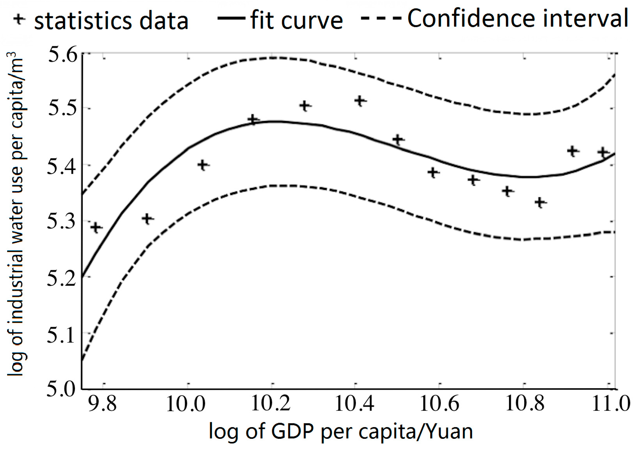
Figure 2 illustrates the fitting curve for water use in the east coastal region to explain the relatively unsatisfying fitting result.

The two last sets of data were inconsistent with the increase-to-decrease trend of EKC, and the data for 2013 and 2014 were relatively different from the data of other years. This disparity is inconsistent with the variation law of curves. The unfitting data were judged preliminarily as outliers, which probably explains the small $R^2$ value. Therefore, the data points for 2013 and 2014 were removed before reconducting the fitting.

Table 5. Fitting parameters and analysis results corrected with the EKC method.

Fitting Parameters	0. China	2. Northern Coastal Region	3. Eastern Coastal Region	6. Middle Yangtze River Region
${\beta }_0$	188.291	283.146	−301.181	230.655
${\beta }_1$	−61.022	−80.174	82.080	−75.631
${\beta }_2$	6.711	7.651	–7.267	8.387
${\beta }_3$	−0.245	−0.243	0.213	−0.308
$R^2$	0.9721	0.9709	0.8475	0.9619
$F$	104.4502	100.2204	12.9702	75.7087
$p$	0.0000	0.0000	0.0030	0.0000
Shape	Inverted U	Declining	Inverted U	Inverted U
Coordinates of Turning Point	(9.8749, 4.6735)	-	(10.3098, 5.4783)	(9.8184, 5.0622)
(Per Capita GDP, Industrial Water use Per Capita)	(19,436,107)	-	(30,025,239)	(18,369,158)

presents the corrected fitting parameters of EKC for the water use and analysis results for China and the three regions.

The statistics and probability in Table 5 indicate that the corrected results are satisfactory. The fitted curve is effective at a confidence level of 99% for each group of data. The $R^2$ value of the eastern coastal region rises to 85% overall, indicating that 86% of the dependent variables can be explained by independent variables with the corrected fitting result.

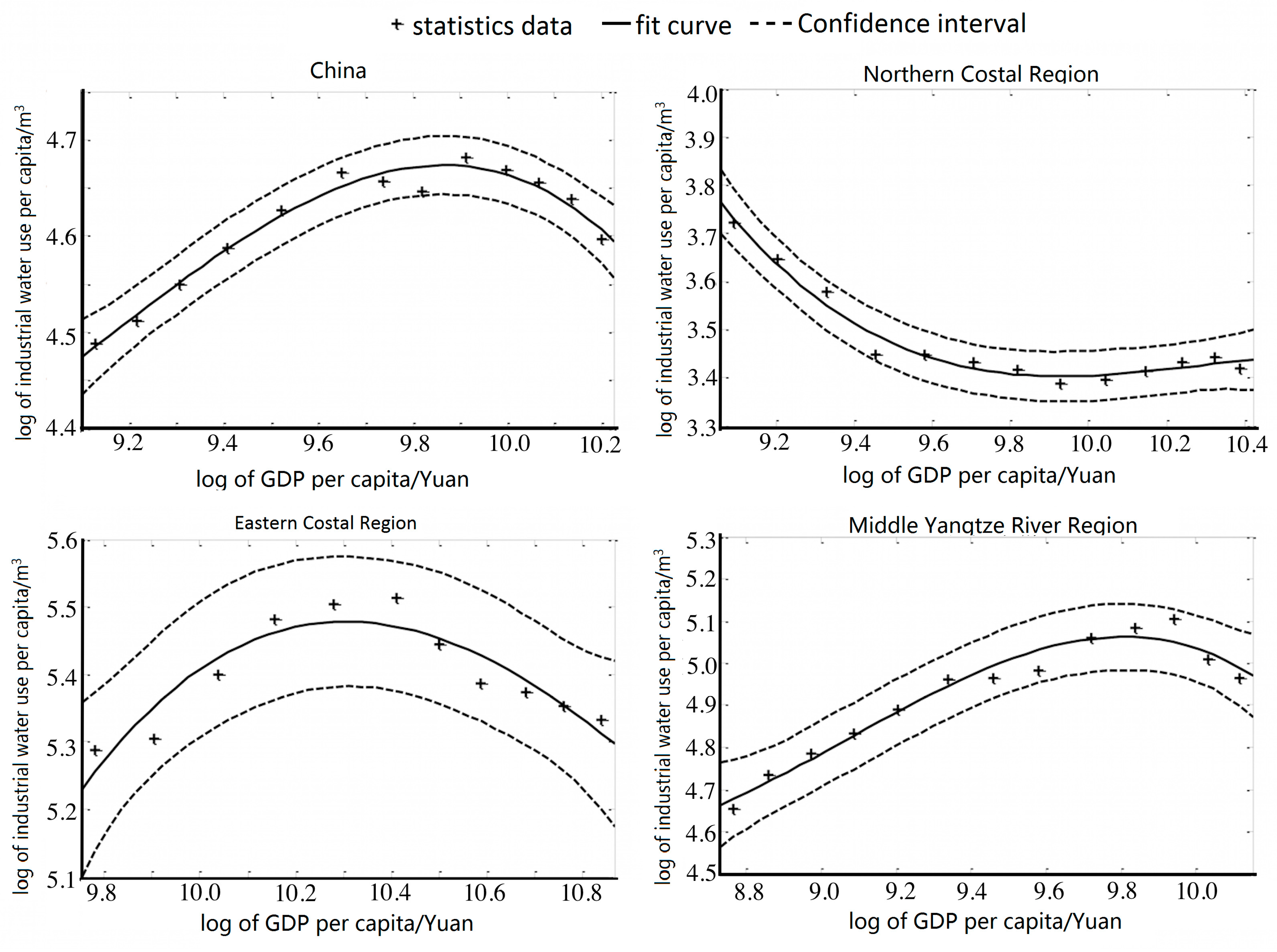
The corrected regression curve formulas for China and the three regions are given in Formulas (2)–(5), with Figure 3 illustrating the charts. The splashes represent the data of different groups, the full-line curves denote fitted curves, the dotted lines above and below the fitted curves signify the confidence level, and the cross of dotted lines is the turning point.

$${\mathrm{logwater}}_0=-0.245{\mathrm{logGDP}}_0^3+6.711{\mathrm{logGDP}}_0^2-61.022{\mathrm{logGDP}}_0+188.291$$

(2)

$${\mathrm{logwater}}_2=-0.243{\mathrm{logGDP}}_2^3+7.651{\mathrm{logGDP}}_2^2-80.174{\mathrm{logGDP}}_2+283.146$$

(3)

$${\mathrm{logwater}}_3=0.213{\mathrm{logGDP}}_3^3-7.267{\mathrm{logGDP}}_3^2+82.080{\mathrm{logGDP}}_3-301.181$$

(4)

$${\mathrm{logwater}}_6=-0.308{\mathrm{logGDP}}_6^3+8.387{\mathrm{logGDP}}_6^2-75.631{\mathrm{logGDP}}_6+230.655$$

(5)

4. Discussion

The results of the parametric regression support the EKC hypothesis overall. The relationship between economic growth and water use displays an inverted U-shape for China and the three regions during the period covered. The per capita industrial water use of the northern coastal region has started to decline. The relationship between per capita industrial water use and GDP showed an inverted U-shaped curve from 2002 to 2014 for China as well as the eastern coastal and middle Yangtze River regions, with the coordinates of the turning points being (9.8749, 4.6735), (10.3098, 5.4783), and (9.8184, 5.0622), respectively. However, the turning point of the northern coastal region was not discovered because of the short period of statistics. In China as well as the eastern coastal and middle Yangtze River regions, the relationship between per capita industrial water use and GDP supports the EKC hypothesis. In Beijing, Tianjin, and Hebei, which are parts of the northern coastal region, economic and industrial development are advanced; thus, their curves exhibit an overall decline during the period of statistics. They may have passed the turning point before the start of the statistical period. The EKC hypothesis should not be rejected in the relationship between per capita industrial water use and GDP of the northern coastal region.

The per capita GDP at the turning point of the inverted U-shaped curve is 18,000–30,000 Yuan (at constant prices from 2000). The turning point of the EKC for per capita industrial water use appears in 2009–2010 for the entire China, in 2006–2007 for the eastern coastal region, and in 2010–2011 for the middle Yangtze River region, with a per capita GDP of 19,436 Yuan, 30,025 Yuan, and 18,369 Yuan, respectively, at the turning point. When the per capita GDP exceeds 2000 Yuan, industrial water use will start to decline along with economic growth in these regions.

Differences exist in the per capita industrial water use at the turning point between 200 and 240 m³. The value is 107 m³, 239 m³ and 158 m³ for the entire China, eastern coastal, and middle Yangtze River regions, respectively, closely relating to their stages of industrial and economic development. Results for the north coastal region show that it has passed the turning point, is on the decline, and has achieved a win–win situation with economic growth and industrial water use decrease. Other regions will also pass the turning point in the short term. For the regions that fail the data test, the EKC hypothesis is not accepted theoretically.

5. Conclusions

The classic EKC theory reveals the economy–pollution relationship and considers that environmental indicators (emissions and other ecological impacts) will increase with the development of the economy, without changes in economic structure and technical process. It is regarded as a scale effect. Along with improvements in technical process and production efficiency, economic further development will not destroy the environment. It is considered as a technical effect. With economic development, more environment requirements will be raised and will contribute to improving ecological quality. Per capita industrial water use will decline along with economic development based on the experience of developed countries. A relationship described by the Kuznets curve can be observed for a number of developed countries.

The EKC for the industrial water use in China was verified through a reduction model according to unit root and co-integration tests—based on the data on per capita industrial water use and GDP of China and the eight economic zones from 2002 to 2014—in order to accurately represent the economic development characteristics of each region, analyze the regions with different features, and obtain results consistent with actual economic development. This study found that increasing industrial water use in China is consistent with EKC characteristics and that an inverted U-shaped relationship exists between per capita industrial water use and GDP. The major reasons for this trend include improvements in water use efficiency resulting from technological innovation and water use transfer attributed to industrial structure upgrades.

Imbalanced regional development will differentiate the turning point for industrial water use in China. During the period studied, China along with the eastern coastal and middle Yangtze River regions experienced their turning point between 2006 and 2011. The northern coastal region is assumed to have passed its turning point before 2002; thus, its per capita industrial water use is constantly declining in the statistics. The difference in the turning points is attributable to the different levels of industrial development and economy of these regions. For instance, the eastern coastal region, including Beijing, Tianjin, Hebei, and Shandong, boasts a high per capita GDP and an advanced economy. Particularly, both Tianjin and Hebei are important industrial cities for China. This region achieved technological breakthroughs and industrial structural adjustments early and experienced an early turning point of the EKC for industrial water use. Other regions will also pass the turning point in the short term and witness a decrease in industrial water use while achieving economic development.

Research on the EKC for industrial water use is highly significant. In the foreseeable future, the economy of China will continue to grow rapidly, the industry share in GDP will keep rising, and the disharmony between economic growth and industrial water use will remain. On 2 April 2015, China released the Water Pollution Prevention and Control Action Plan, requiring the adjustment of industrial structures and the optimization of spatial arrangements. This plan aims to promote cyclic development, control total water use, improve water use efficiency, conserve industrial water effectively, popularize and demonstrate applicable technology, develop cutting-edge technology, intensify water pollution control, and assure national water security. This study provides important thoughts and lessons for collaborative research on the relationship between industrial water use and economic development. It is also helpful in balancing the relationship between industrial water use and economic development. The central government should focus on central and western regions when creating policies for water resource management and technological development to improve their industrial water use efficiency. The government should also promote the deceleration of their water use consumption while shrinking the economic gap between the mid-western regions and mid-eastern regions. In addition, the government should create multiple policies to promote economic development and remove difficulties resulting from increasing industrial water use, pass the turning point, and achieve a win–win situation at the soonest possible time.

The results presented in this study are indefinite because the data were limited, and factors such as the complicated population, technical advancements, and policy adjustments could not be analyzed in the model. Future research should consider the selection of data indices and the scope of panel data in order to provide detailed analysis and discussion.

References

- World Water Counsil. World Water Vision 2025; Earthscan Publications Ltd.: London, UK, 2000. [Google Scholar]
- National Bureau of Statistics. China Statistical Yearbook 2015; China Statistics Press: Beijing, China, 2015.
- The World Bank. China: Air, Land and Water-Environmental Priorities for a New Millennium; The World Bank: Washington, WA, USA, 2001. [Google Scholar]
- Kuznets, S. Economic growth and income inequality. Am. Econ. Rev. 1955, 45, 1–28. [Google Scholar]
- Panayotou, T. Empirical Tests and Policy Analysis of Environmental Degradation at Different Stages of Economic Development; International Labour Office: Geneva, Switzerland, 1993. [Google Scholar]
- Selden, T.M.; Song, D. Environmental quality and development: Is there a Kuznets curve for air pollution emissions? J. Environ. Econ. Manag. 1994, 27, 147–162. [Google Scholar] [CrossRef]
- Luzzati, T.; Orsini, M. Investigating the energy-environmental kuznets curve. Energy 2009, 34, 291–300. [Google Scholar] [CrossRef]
- Rock, M.T. Freshwater use, freshwater scarcity, and socioeconomic development. J. Environ. Dev. 1998, 7, 278–301. [Google Scholar] [CrossRef]
- Katz, D. Water use and economic growth: Reconsidering the environmental kuznets curve relationship. J. Clean. Prod. 2015, 88, 205–213. [Google Scholar] [CrossRef]
- Gleick, P. Water Use. Annu. Rev. Environ. Resour. 2003, 28, 275–314. [Google Scholar] [CrossRef]
- Hemati, A.; Mehrara, M.; Sayehmiri, A. New vision on the relationship between income and water withdrawal in industry sector. Nat. Resour. 2011, 2, 191–196. [Google Scholar] [CrossRef]
- Jia, S.F.; Zhang, S.F.; Yang, H. The relationship between industrial water consumption and economic development—Kuznets curve for water use. J. Nat. Resour. 2004, 19, 279–284. [Google Scholar]
- Li, Q.; Wang, L.F.; Jia, X.M. Research on the relationship between water resource utilization and economic growth based on EKC. Sci. Technol. Ind. 2015, 15, 133–136. [Google Scholar]
- Zhang, B.B.; Shen, M.H. Analysis on the Kuznets curve for industrial water consumption. Resour. Sci. 2016, 38, 0102–0109. [Google Scholar]
- Bacon, D.W.; Watts, D.G. Estimating the transition between two intersecting straight lines. Biometrika 1971, 58, 525–534. [Google Scholar] [CrossRef]
- Teräsvirta, T. Modeling economic relationships with smooth transition regressions. In Handbook of Applied Economic Statistics; Marcel Dekker, Inc.: New York, NY, USA, 1998. [Google Scholar]
- Matthew, A.C. Economic growth and water use. Appl. Econ. Lett. 2004, 11, 1–4. [Google Scholar]
- Katz, D.L. Water, Economic Growth, and Conflict: Three Studies; University of Michigan: Michigan, MI, USA, 2008. [Google Scholar]
- Bhattarai, M. Irrigation Kuznets Curve Governance and Dynamics of Irrigation Development: A Global Cross-Country Analysis from 1972 to 1991; International Water Management Institute: Colombo, Sri Lanka, 2004. [Google Scholar]
- Duarte, R.; Pinilla, V.; Serrano, A. Is there an environmental kuznets curve for water use? A panel smooth transition regression approach. Econ. Model. 2013, 31, 518–527. [Google Scholar] [CrossRef]
- Fouquau, J.; Destais, G.; Christophe, H. Energy demand models: A threshold panel specification of the “Kuznets curve”. Appl. Econ. Lett. 2009, 16, 1241–1244. [Google Scholar] [CrossRef]
- List, J.A.; Gallet, C.A. The environmental Kuznets curve: Does one size fit all? Ecol. Econ. 1999, 31, 409–423. [Google Scholar] [CrossRef]
- Grossman, G.M.; Krueger, A.B. Economic growth and the environment. Q. J. Econ. 1995, 110, 353–378. [Google Scholar] [CrossRef]
- Moomaw, W.R.; Unruh, G.C. Are environmental Kuznets curves misleading us? The case of CO2 emissions. Environ. Dev. Econ. 1997, 2, 451–463. [Google Scholar] [CrossRef]
- Stern, D.I. The rise and fall of the environmental Kuznets curve. World Dev. 2014, 32, 1419–1439. [Google Scholar] [CrossRef]
- Li, S.T.; Hou, Y.Z.; Feng, J. Strategic thinking and policy measures for achieving regional coordinated development. Shanghai Invest. 2005, 7, 4–8. [Google Scholar]
- Li, S.T.; Hou, Y.Z. Mainland China: Division of eight social-economic regions. Forw. Position Econ. 2003, 5, 12–15. [Google Scholar]
- Granger, C.W.J.; Newbold, P. Spurious regressions in econometrics. J. Econ. 1974, 2, 111–120. [Google Scholar] [CrossRef]
- Dickey, D.A.; Fuller, W.A. Distribution of the estimators for autore-gressive time series with a unit root. J. Am. Stat. Assoc. 1979, 74, 427–431. [Google Scholar]
- Engle, R.; Granger, C. Cointegration and error correction: Representation, estimation, and testing. Econometrica 1987, 55, 251–276. [Google Scholar] [CrossRef]
- Johansen, S.; Juselius, K. Maximum likelihood estimation and inference on cointegration-with applications to the demand for money. Oxf. Bull. Econ. Stat. 1990, 52, 169–210. [Google Scholar] [CrossRef]
Figure 1.
Relationship between per capita industrial water use and GDP of eight economic zones in China (2014).
Figure 2.
Estimated EKC of the eastern coastal region.
Figure 3.
Estimated EKC curve of China, northern coastal, eastern coastal, and middle Yangtze River regions (corrected).