Dependence of Sediment Suspension Viscosity on Solid Concentration: A Simple General Equation


College of Water Sciences, Beijing Normal University, Beijing 100875, China
*
Author to whom correspondence should be addressed.
Water 2017, 9(7), 474; https://doi.org/10.3390/w9070474
Submission received: 27 May 2017
/
Revised: 24 June 2017
/
Accepted: 26 June 2017
/
Published: 28 June 2017
Abstract
:In this study, a simple and new parametric equation is proposed that describes the relative viscosity of a suspension as a function of suspended solid concentration, covering a range from very dilute to highly concentrated states, based on Costa (2005). The proposed viscosity law depends mainly on the solid volumetric concentration and maximum packing fraction at which a regime transition occurs. Furthermore, the viscosity of dilute as well as a highly-concentrated kaolinite suspension (in excess of 40% and lower than 50%) was measured in a coaxial cylinder rheometer. The proposed formula shows a capability of fitting the measured bulk viscosity into the hyper-concentrated regime in the experiment. Finally, the proposed equation could also be found to show a good fitting relationship with published experimental results on partially crystallised Li2Si2O5 melt and partially melted granite with solid contents from 75% to 95%.
1. Introduction
Cohesive sediment commonly exists in harbour, estuary and coastal waters all over the world [1]. Understanding cohesive sediment transport is important for engineering projects related to dredging operations of navigation channels, morphological changes of shorelines and water quality control in estuarine and coastal areas [2,3,4,5,6]. Transport of cohesive sediment occurs both in the water column and in the near-bed water layer. For the latter, the sediment concentration is often very high and the term “fluid mud” has been used to describe it [7,8,9]. Motion of fluid mud layer, which is caused by water current and wave, may lead to a high sediment transport rate [6]. In order to predict the onset and motion characteristics of the fluid mud layer, it may be important to understand their rheological properties (including bulk viscosity and yield stress) [6,10,11]. Furthermore, the viscosity of the fluid mud layer has been shown to be important for evaluation of the entrainment rate of sediment between the fluid mud layer and the overlying water layer [12,13]. Meanwhile, the hindering settling velocities of cohesive sediment flocs, which is an important variable for calculation of suspended sediment flux, are also related to the viscosity of water-sediment suspension when sediment concentration is high enough [14,15]. Thus, investigating rheological properties of the cohesive sediment mixture especially in the case of a highly concentrated suspension, where no experimental data are seemingly available [2,3,14], could be helpful to better understand cohesive sediment transport in estuarine and coastal waters. This study focuses on the suspension viscosity. The suspension viscosity, not limited to the sediment mixture, is affected by particle concentration, shear rate, particle shape, particle size distribution and particle deformability [16,17,18]. Among these factors, the dependence of suspension viscosity on the particle concentration is of great interest in the sediment field [2,3,19,20]. Experiments have been performed to study this relationship, and some models have been used to describe it [21,22,23,24,25,26]. However, a simple relationship may not exist because the particle in a suspending medium can be subject to hydrodynamic, Brownian, colloidal force and other effects, which are not easily modelled in a simple form [16,27,28,29].
Some proposed models characterizing the suspension viscosity-solid particle concentration relationship are simply summarized as follows. In the case of a notably dilute suspension of spherical non-interacting mono-disperse particles, Einstein [30] derived an analytical solution to describe the relative viscosity of the suspension () (defined as the ratio of the suspension viscosity and viscosity of the suspended medium) as a function of solid fraction,
where is the volumetric concentration (or fraction) of particles, defined as the volume occupied by particles and total volume of the suspension, and is the Einstein coefficient with a theoretical value of 2.5 for hard spheres. Batchelor [31] theoretically extended this relationship to the second order,
where = 6.2 for Brownian suspensions in any flow, and = 7.6 for non-Brownian suspensions in a straining flow. When particle concentrations are high, particle crowding causes hydrodynamic interactions among particles, which results in large positive deviations from the viscosity value of highly concentrated suspensions from Equations (1) and (2) [16].
For the case of a highly concentrated suspension, Roscoe [32] proposed the following expression starting from the Einstein equation,
where the new parameter is the maximum packing concentration of particles, at which there is no longer sufficient fluid to lubricate relative particle motion, and the incompressible solid would prevent any flow [21]. Its value varies depending on various factors, such as the variation of particles from mono-size, and the geometric arrangement of particles [16,17,18].
Equations (1)–(3) apply only to the suspension in which non-cohesive particles are suspended. In such cases, Boyer et al. [25] proposed the following —dependent constitutive laws of dense suspensions, by modelling the friction law of dense suspension as the sum of two contributions coming from contact between particles and hydrodynamic stresses between particle and surrounding fluid,
wit , an , and were suggested in Boyer et al. [25]. Later, by conducting numerical simulation of an athermal dense suspension under shear, Trulsson et al. [26] showed that the Newtonian and Bagnoldian regimes of dense suspension rheology could be unified as a function of a single dimensionless number.
On the other hand, some rheologists have proposed many semi-empirical or empirical models to fit the observed experimental results, considering Equation (1) as a starting point [21,22,23,24]. A frequently adopted model that fits experimental data well is the semi-empirical expression, introduced by Krieger and Dougherty [21] for mono-dispersed suspensions,
For very dilute suspensions (), this expression can be reduced to the Einstein equation: . Some experiments have shown that the exponent of Equation (5) (i.e., ) is always approximately two for many suspensions [33,34]. The exact particle concentration () at which there is no fluid to lubricate particle motion for a system of particles remains a matter of debate [16,34], and its determination appears to be an open problem. In many experiments, was commonly used as an adjustable parameter, so that Equation (5) can provide an excellent fitting relationship with the experimental data. Other fitting expressions proposed by some authors also used as an adjustable parameter, like for example, the equation proposed by Chong et al. [22],
and the proposed equation by Dabak and Yucel [23],
After summarizing the common form of some semi-empirical fitting expressions, Liu [24] proposed a more general formula to describe the viscosity behaviour of suspensions,
with , where and are the slope and intercept values of the straight line vs. relation, which must be experimentally determined, and is a flow-dependent suspension-specific parameter (the author used = 2). The term is clearly interpreted as the effective space available for particles to move in the matrix fluid.
The majority of the proposed models for a highly concentrated suspension assume that there is a critical solid concentration at which the incompressible solid would prevent any flow. It may be reasonable to consider that when the solid concentration increases across , the suspension experiences a transition of rheological regime: the suspension rheology changes from being primarily determined by the liquid phase to exhibiting remarkably non-Newtonian behaviour with a yield stress [19,20,28,29,35]. In the latter regime, the rheology is much more complex than the former regime. Costa noticed this transition of rheological regime of the suspension, and further proposed a general parameterization to characterize the suspension viscosity-solid concentration relationship as follows,
where , and are three adjustable parameters. According to Equation (9), the suspension viscosity initially increases (here we term it an initial linear increasing regime), and then experiences an intermediate increasing process (here called an intermediate increasing regime) with the increasing solid particle concentration. However, with the continual increase of solid concentration, the suspension viscosity predicted by Equation (9) exhibits an asymptotic behaviour and finally reaches a steady state for a very high solid concentration. The assumption that the highly-concentrated suspension has a fixed viscosity value seems questionable. In fact, our experimental works (as discussed in Section 4) on the viscosity of kaolinite suspension across a certain range in particle concentration shows that the suspension viscosity increases with increasing solid concentration. Moreover, measured data for viscosity-crystal fraction relationship in partially crystallised Li2Si2O5 and observation data of partially melted granite with solid content from 75% to 95% also clearly indicated this increasing behaviour when crystal fraction exceeds the maximum packing concentration (as also discussed in Section 4) [36,37]. Costa [35] has used these data to verify Equation (9), but neglecting the increasing behaviour of the suspension viscosity at a high solid concentration. Therefore, a more general parameterization may be necessary to describe the complex behaviour of the suspension, covering a range of solid concentration from very dilute to highly concentrated states.
This study attempts to identify a more general relationship between and , based on Costa [35]. The proposed equation is intended to not only describe the aforementioned rheological transitions of the suspension (especially the increasing trend at high solid concentration), but also to provide adjustable parameters that can be easily interpreted from a physical perspective and that reduce to the Einstein equation for a very dilute suspension (), similar to previously proposed models. This paper is arranged as follows. Section 2 proposes a simple new parameterization. An experiment that measures viscosity-solid concentration values of a water-kaolinite suspension, performed to verify the validity of the proposed equation, is detailed in Section 3. Section 4 presents the comparisons of the proposed equation with experimental results in this study and previously published experimental results on partially crystallised Li2Si2O5 and partially melted granite. Finally, some concluding remarks are presented in Section 5.
2. Simple Newly-Proposed Equation
In order to reproduce the continually increasing behaviour of for higher than , we simply add a power function of solid concentration (up to second order) on the right-handed side of Costa equation, so that the final form of the suspension viscosity as a function of solid concentration becomes
where is an exponent (), and is the non-dimensional form of the solid concentration. The error function is the integral of the Gaussian distribution: at , and it shows a rapid and an asymptotic increasing behaviour with continually increasing . Its Taylor expansion near is: .
For very dilute suspensions (), the argument of the error function approaches , and further the error function becomes by virtue of the Taylor expansion. Thus the curly bracket part of the right-handed side of Equation (10) could reduce to as . Meanwhile, the square bracket part of the right-handed side of Equation (10) approaches unity when . Therefore, the − parameterisation for very dilute suspensions becomes: , which is similar to well-established Einstein equation valid for dilute suspensions, where the Einstein coefficient becomes , and could be regarded as a correction coefficient due to the non-linear term in the argument of the error function. For highly concentrated solid-liquid systems (large ), the error function approaches unity with increasing , and the curly bracket part of the right-handed side of Equation (10) becomes . Moreover, the square bracket part exhibits an increasing behaviour with . As a result, for highly concentrated solid-liquid systems shows an expected increasing trend with increasing .
A graphical analysis is employed to explore the physical explanations of all parameters incorporated in Equation (10), as shown in Figure 1. As discussed previously, and shown in Figure 1a, the parameter controls the viscosity value from which the suspension exhibits remarkably non-Newtonian behaviour with a yield stress, and the continually increasing regime of with for large begins. Parameter (Figure 1b), controls the slope of the initial linear regime of viscosity (as shown in reduced form of Equation (10) as ), and partially determines the slope curve between the initial linear and continually increasing regime. Parameter (Figure 1c), similar to parameter , determines the width of the intermediate increasing regime and can be regarded as a measure of the rapidity to reach the continually increasing regime from the initial linear increasing regime. A smaller parameter leads to a larger width of the intermediate increasing regime. The newly-added parameter in this study primarily controls the rate at which the viscosity increases with particle concentration in the continually increasing regime, as shown in Figure 1d.
3. Experiment Introduction
In order to avoid discussing the effect of particle mineral composition on the suspension [38], this study simply adopted kaolinite (China clay) suspended in deionized water to form the solid–liquid suspension. The grain size distribution of the kaolinite sample was measured using a laser diffraction particle size analyser (Helos & Rodos; produced by Sympatec Corporation, Clausthal-Zellerfeld, Germany), and more information about measurement method of this instrument (including dry dispersion for sample powder) can be found on the website [39]. As shown in Figure 2, the median size of this sample was 3.71 μm with a range of 0.5–18.5 μm. The kaolinite concentration in the suspension was chosen to be in the range of 1.88 × 10⁻³ to 0.48 in this study, covering a very dilute to highly concentrated state [2,3,4]. The upper limit value of kaolinite concentration (i.e., 0.48) is determined based on the experimental finding that the suspension shear stress value, when particle concentrations are higher than 0.48, exceeds the upper limit value of measuring scope of the rheometer in this experiment.
Rheological properties of the water-kaolinite suspension were measured using a Brookfield RST-CCT40 rheometer(Brookfield Engineering Laboratories Incorporation, Middleboro, MA, USA) This rheometer mainly consists of a touch screen, an electronic unit and a measuring drive, which is coupled to coaxial cylinder systems and the Rheo3000 software (Rheo3000 1.2.1395.1, Brookfield Engineering Laboratories Incorporation, Middleboro, MA, USA. When a coaxial cylinder spindle, which consists of a shaft and a measuring bob, is immersed in the sample cup (filled with the water-kaolinite sample, volume 68.5 mL) and driven at different angular velocities, the torques experienced by the spindle are detected. The angular velocity of the spindle is converted to shear rate in the suspension using a shear rate factor, and the torque corresponds to shear stress using the shear stress factor. A comprehensive introduction to the rheometer configuration and measuring system can be found on the website [40]. The Rheo 3000 software coupled with a personal computer was used to remotely manipulate the rheometer. The shear rate was set to be 2.16–644.41 , covering the low to high shear conditions in this experiment [3].
After the water-kaolinite suspension was prepared for a kaolinite concentration of , it was gently injected into the sample cup, and the rheological measurement was initiated. The angular velocity of the spindle was adjusted to gradually increase over 100 s, resulting in a shear rate range of 2.16–644.41 The torque (corresponding to the shear stress) that the spindle experienced was measured. The measuring system plotted the shear stress-shear rate relationship in real time, and presented the suspension viscosity value. For every kaolinite concentration, we repeated the procedure, from preparing the sample to measuring rheological characteristics, three times. The viscosity value of the water-kaolinite suspension was finally determined as the mean of the three measured viscosity values. For some water-kaolinite suspensions, we carefully monitored the solid particle concentration before the experiment was initiated and again after the experiment was completed, and found that there was no obvious variation for particle concentration due to the possible appearance of the sedimentation effect of the kaolinite particle [19]. Before all experiments, the viscosity of deionized water was also measured. The experimental temperature was 21 ± 0.5 °C.
4. Comparison with Experimental Results and Published Observational Data
4.1. Comparison with Experimental Results
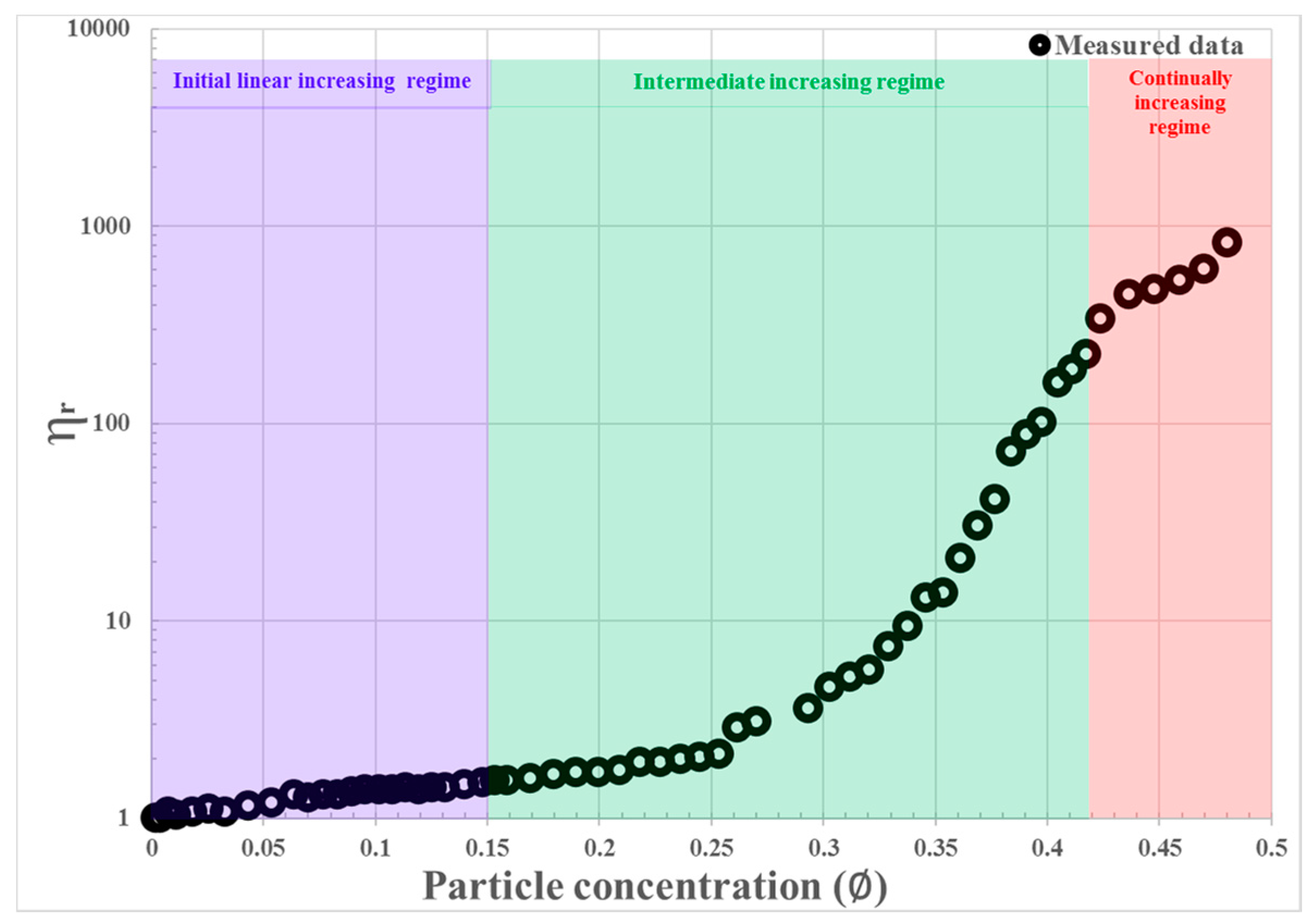
Figure 3 shows the measured relative viscosity values of the water-kaolinite suspension for particle concentrations from 1.88 × 10⁻³ to 0.48. With increasing , first increased linearly (0 < < 0.15) (as shown by blue background colour in Figure 3), then showed intermediate increasing behaviour (0.15 < < 0.42) (as shown by the green background colour), and finally a continuous increasing trend (0.42 < < 0.48) (as shown by the red background colour). The presence of the continually increasing regime during this experiment may indicate complicated rheological properties of the highly concentrated suspension, which exhibited obvious non-Newtonian characteristics and behaved as a solid with applied stress.
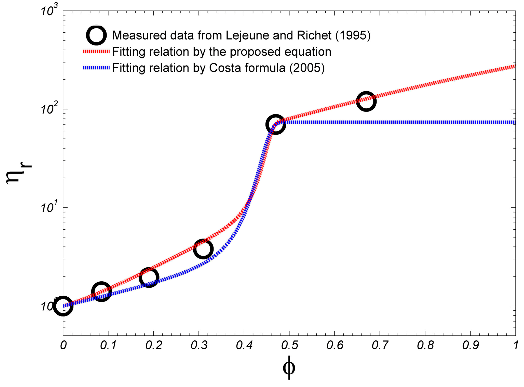
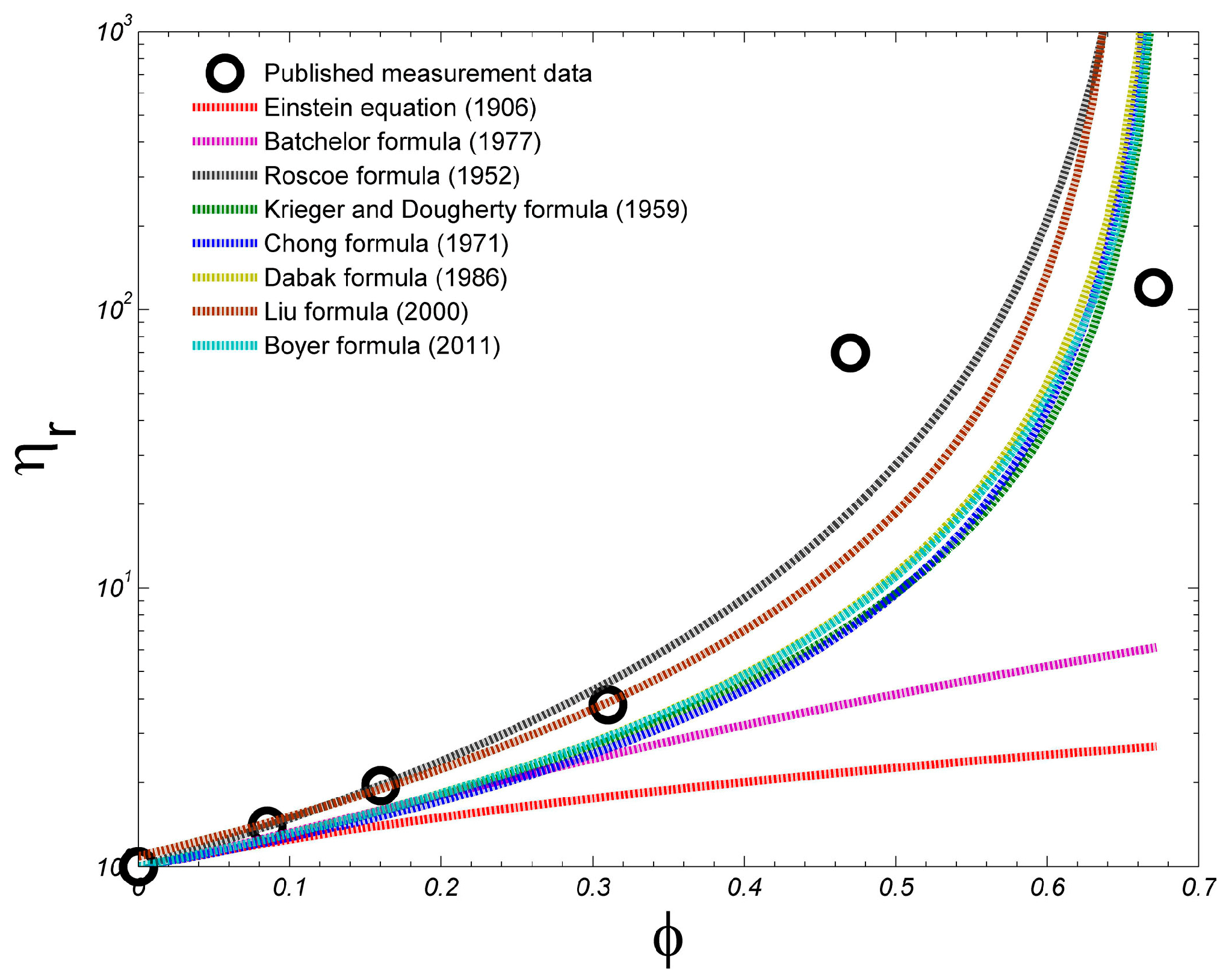
We attempt to fit these measured data using the proposed equation and the formula already proposed by Costa [35], as well as published formulae proposed by other authors, as shown in Figure 4. Goodness of fit is measured with the correlation coefficient, , defined as , and normalized root mean square error, NRMSE, defined as , where and are the modelled and observed points, respectively, and is the number of observed points. Goodness of fit increases as increases and NRMSE decreases. As presented in Table 1, in general, the proposed equation provides the best fit with the measured data, because all four adjustable parameters have been incorporated, and Costa formula also exhibits a better fit result. They are followed by the Krieger and Dougherty formula [21], which gives a high of 0.73; the Boyer formula [25] provides a small NRMSE value equal to 0.14. As observed in Figure 4, with increasing , all formulae predict the viscosity value well for 0 < < 0.05; when reaches 0.1, the Roscoe formula [32] and Liu formula [24] clearly deviate from the measured viscosity values. As approaches 0.15, the Chong formula [22] begins to overestimate the viscosity value, and then underestimates it from = 0.33. For 0.2 < < 0.25, the Dabak [23] and Krieger and Dougherty [21] formulae slightly overestimate the suspension viscosity. The Dabak formula [23] begins to underestimate the viscosity from = 0.3 on, and from = 0.25 on, the Krieger and Dougherty formula [21] starts to underestimate the viscosity. For 0 < < 0.25, the Batchelor formula [31] still provides a better fit effect to measured data, whereas the Einstein equation [30] still underestimates the suspension viscosity value from = 0.1 on. Across the entire range of solid concentration, the Boyer formula [25] is still very close to the Chong formula [22] except for a narrow range of 0.45 < < 0.48, during which the viscosity values predicted by the Chong formula [22] are slightly larger than those by the Boyer formula [25].
The Costa formula [35] that contains three adjustable parameters can fit the initial increasing regime and intermediate increasing regime of suspension viscosity value as a function of solid concentration well. However, as solid concentration exceeds 0.42 (the highly-concentrated suspension starts to exhibit obvious non-Newtonian characteristics during the experiment), it simply tackles the suspension viscosity-solid concentration relationship as a steady state. In fact, when 0.42 < < 0.48, note that the vertical axis is logarithmic coordinate in Figure 4, the suspension viscosity rises rapidly with increasing solid concentration . The proposed formula is capable of modelling this continual increasing regime of suspension viscosity with solid concentration with the cost of adding another new adjustable parameter.
4.2. Comparison with Published Observational Data
To the best of our knowledge, few measured viscosity values for water-sediment suspensions at high solid concentrations are available in the sediment research field, and it is possible that the rheometer does not work properly at high volumetric concentrations because of the critical yield stress, particle migration and non-homogeneous suspension [16,41]. To further confirm the validity of the proposed equation, we attempt to use two groups of previously-published measurement data for high solid concentrations that were introduced by Costa [35].
The first group of published data was conducted by Lejeune and Richet [37]. They measured the viscosity of partially crystallized Li2Si2O5 under uniaxial compression as a function of crystal volumetric concentration. The Li2Si2O5 melt contains small ellipsoidal crystals. Their experimental results suggested that the rheology of the melts is primarily determined by the crystal fraction, even though additional measurements would be helpful to determine the possible influence of other factors, such as the size distribution or shape of inclusions.
Figure 5 shows the measured viscosity-crystal fraction relationship for a partially crystallized Li2Si2O5 melt. A comparison between measured data and predicted values by the proposed equation and that between measured data and predicted values by the Costa formula are also presented in this figure. The agreement with the proposed formula is fairly good, with an value of 0.99 and an NRMSE value of 0.03, whereas the Costa formula also gives a good fit effect with an value of 0.92 and an NRMSE value of 0.16. However, the Costa formula neglects the increasing behaviour of the melt viscosity as the crystal volumetric concentration increases from 0.47 to 0.67, and simply regards it as a plateau of viscosity with solid concentration. In contrast, the proposed formula captures the increasing characteristic of the melt viscosity-crystal concentration relationship. Finally, it should be pointed out that there are very limited experimental data points in this figure to calibrate the proposed equation; in particular, there are no available measured results for larger than 0.67. More experimental results at high solid concentrations to calibrate the proposed equation are necessary in future studies.
We also compare these measured data with some published formulae proposed by other authors, as shown in Figure 6, and Table 2 shows goodness values of fitting for these published formulae. Since the Roscoe formula, the Krieger and Dougherty formula, the Chong formula, the Dabak formula, the Liu formula and the Boyer formula deviate greatly from the measured viscosity value at = 0.67, in general the Batchelor formula provides the best fit to measured data with an value of 0.94 and an NRMSE value of 0.45 among such formulae. For 0 < < 0.31, the Liu formula fits the measured data very well, followed by the Roscoe formula, whereas the rest formulae still underestimate the measured viscosity values.
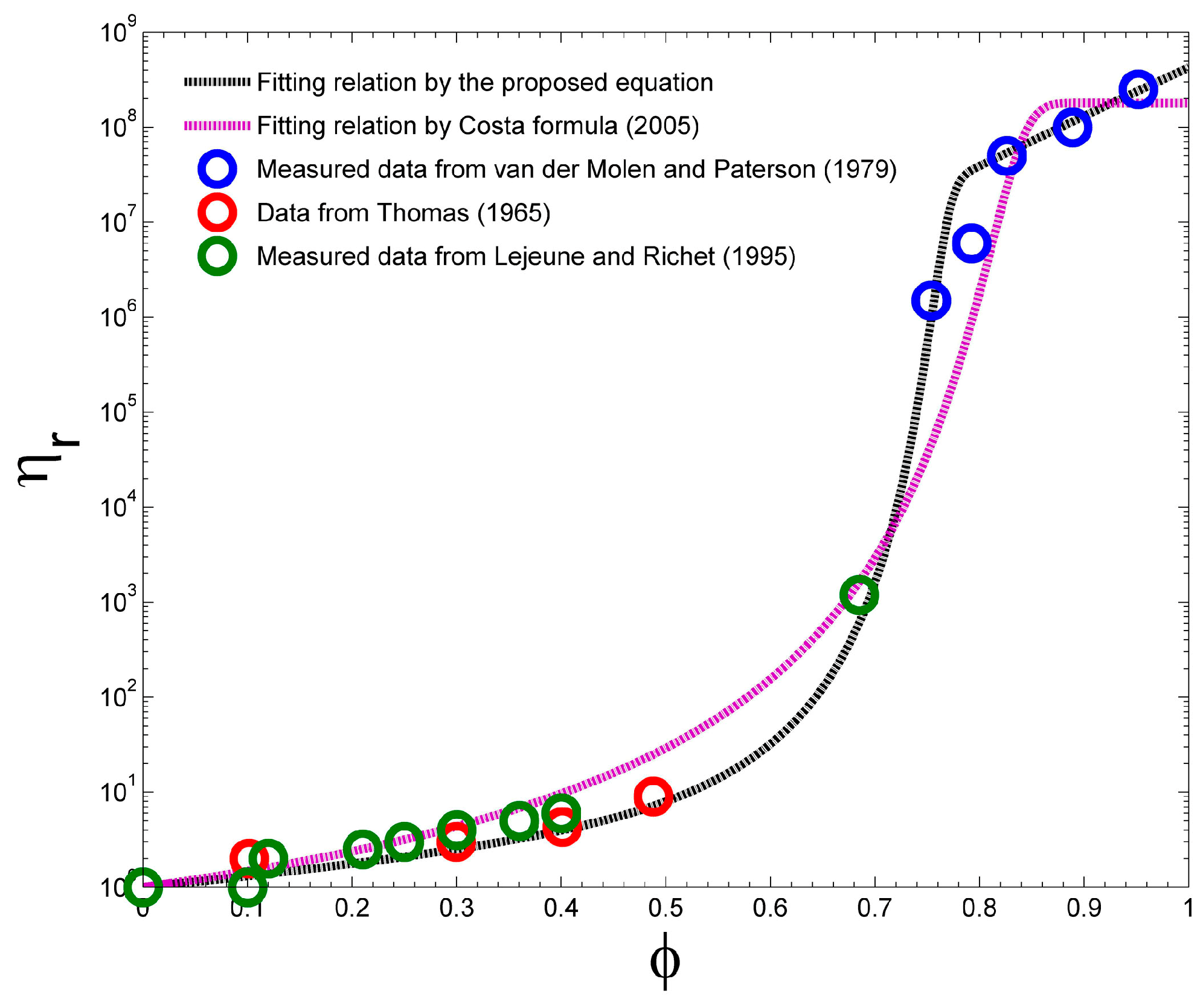
The second group of published data was mainly conducted by van der Molen and Paterson [36]. They investigated the deformation of partially melted granite with solid concentrations from 75% to 95% at 800 and 300 MPa confining pressure and measured viscosity-solid fraction values for partially melted granite. Their measurement results suggested that the critical crystal concentration differentiating granular-framework-controlled flow behaviour from the suspension-like behaviour could be around 0.72. Measured viscosity-crystal fraction values at low solid concentrations for partially crystallized Mg3Al2Si3O12 melt by Lejeune and Richet [37] (for the Mg3Al2Si3O12 melt, crystals are well rounded), and other viscosity-solid fraction values for uniform spherical particles by Thomas [42] were also incorporated into this group of published data in order to make a simple comparison between the available experimental results and the proposed equation [35], although these experimental data are limited and their sources are not coherent.
Figure 7 shows the comparisons of these measurement data with the proposed formula in this study and also with the Costa formula. Fitting by the proposed formula has an value of 0.98 and an NRMSE value of 0.03, whereas the Costa formula only has an value of 0.82 and an NRMSE value of 0.10. As solid concentration increases from 0 to 0.3, the Costa formula agrees with the measured viscosity value slightly better than the proposed formula. For 0.3 < < 0.69, the Costa formula overestimates the viscosity values, whereas it underestimates the viscosity value for 0.69 < < 0.83. When solid concentration continually increases from 0.83 to 0.95, the Costa formula simply adopts a steady state value of the highly-concentrated suspension viscosity, which do not characterize the continually increasing trend of the viscosity with solid concentration. In this respect, the proposed formula is capable of characterizing this behaviour.
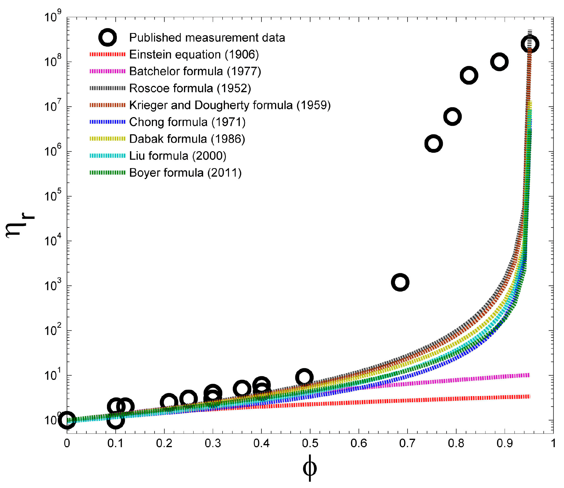
The comparisons of measured data with some published formulae are shown in Figure 8. Table 3 shows goodness values of fitting for these published formulae, among which, the Krieger and Dougherty formula [21] provides the best fit to published experimental data, with an value of 0.83 and a lowest NRMSE value of 0.12.
Finally, although the proposed equation in this study has a good fitting relationship with the measured data and some published experimental data, there is an intrinsic limitation: there are four adjustable parameters incorporated within it, and it has no simple form, whereas the previously proposed published formulae do. Future work should be aimed at simplifying the proposed equation and further improving its applicability to fit experimental or observational results.
5. Concluding Remarks
In this study, a general equation was proposed that describes the relative viscosity of a suspension as a function of suspended solid concentration, covering a range from very dilute to highly concentrated states, based on Costa [35]. The viscosity of dilute as well as a highly concentrated kaolinite suspension (in excess of 40% and lower than 50%) was measured in a coaxial cylinder rheometer. A comparison with measured viscosity-solid concentration values showed the validity of the proposed equation. The proposed equation also showed a good fitting relationship with published rheological behaviours of partially crystallised Li2Si2O5 and Mg3Al2Si3O12. Simplifying the proposed equation and further improving its fit with experimental or observational results should be the goal of future research.
Acknowledgments
This work is supported by the National Natural Science Foundation of China (Number: 51509004).
Author Contributions
Zhongfan Zhu had the original idea, developed the models, carried out experiments, analyzed the results and wrote the paper. Hongrui Wang joined the discussion of experimental results and contributed to the revision of the original manuscript. Dingzhi Peng contributed to the revised one of the original manuscript.
Conflicts of Interest
The author declare no conflict of interest.
References
- Dean, R.G.; Dalrymple, R.A. Coastal Processes with Engineering Applications, 1st ed.; Cambridge University Press: Cambridge, UK, 2002; pp. 471–478. ISBN 0521602750. [Google Scholar]
- Julien, P.Y.; Lan, Y. Rheology of hyperconcentrations. J. Hydraul. Eng. 1991, 117, 346–353. [Google Scholar] [CrossRef]
- Huang, Z.; Aode, H. A laboratory study of rheological properties of mudflows in Hangzhou Bay, China. Int. J. Sediment Res. 2009, 24, 410–424. [Google Scholar] [CrossRef]
- Bai, Y.C.; Ng, C.O.; Shen, H.T.; Wang, S.Y. Rheological properties and incipient motion of cohesive sediment in the Haihe Estuary of China. China Ocean Eng. 2002, 16, 483–498. [Google Scholar]
- Huang, X.; Garcia, M.H. A Herschel-Bulkley model for mud flow down a slope. J. Fluid Mech. 1998, 374, 305–333. [Google Scholar] [CrossRef]
- Van Kessel, T.; Blom, C. Rhelogy of cohesive sediments: Comparison between a natural and an artificial mud. J. Hydraul. Res. 1998, 36, 591–612. [Google Scholar] [CrossRef]
- Mehta, A.J. Understanding fluid mud in a dynamic environment. Geo-Mar. Lett. 1991, 11, 113–118. [Google Scholar] [CrossRef]
- Shi, Z. Acoustic observations of fluid mud and interfacial waves, Hangzhou Bay, China. J. Coast. Res. 1998, 14, 1348–1353. [Google Scholar]
- Mehta, A.J. Mudshore dynamics and controls. In Muddy Coasts of the World: Processes, Deposits and Function, 1st ed.; Healy, T., Wang, Y., Healy, J.A., Eds.; Elsevier: Amsterdam, The Netherlands, 2002; pp. 19–60. ISBN 0-444-510192. [Google Scholar]
- Faas, R.W.; Wartel, S.I. Rheological properties of sediment suspensions from Eckernforde and Kieler Forde bays, western Baltic Sea. Int. J. Sediment Res. 2006, 21, 24–41. [Google Scholar]
- Granboulan, J.; Feral, A.; Villerot, M.; Jouanneau, J.M. Study of the sedimentological and rheological properties of fluid mud in the fluvio-estuarine system of the Gironde estuary. Ocean Coast. Manag. 1989, 12, 23–46. [Google Scholar] [CrossRef]
- Kranenburg, C.; Winterwerp, J.C. Erosion of fluid mud layers. I: Entrainment model. J. Hydraul. Eng. 1997, 123, 504–511. [Google Scholar] [CrossRef]
- Winterwerp, J.C.; Kranenburg, C. Erosion of fluid mud layers. II: Experiments and model validation. J. Hydraul. Eng. 1997, 123, 512–519. [Google Scholar] [CrossRef]
- Winterwerp, J.C. On the flocculation and settling velocity of estuarine mud. Cont. Shelf Res. 2002, 22, 1339–1360. [Google Scholar] [CrossRef]
- Dankers, P.J.T.; Winterwerp, J.C. Hindered settling of mud flocs: Theory and validation. Cont. Shelf Res. 2007, 27, 1893–1907. [Google Scholar] [CrossRef]
- Genovese, D.B. Shear rheology of hard-sphere, dispersed, and aggregated suspensions, and filler-matrix composites. Adv. Colloid Interface Sci. 2012, 171, 1–16. [Google Scholar] [CrossRef] [PubMed]
- Stickel, J.J.; Powell, R.L. Fluid mechanics and rheology of dense suspensions. Annu. Rev. Fluid Mech. 2005, 37, 129–149. [Google Scholar] [CrossRef]
- Mueller, S.; Llewellin, E.W.; Mader, H.M. The rheology of suspensions of solid particles. Proc. R. Soc. Lond. 2010, 466, 1201–1228. [Google Scholar] [CrossRef]
- Coussot, P. Structural similarity and transition from Newtonian to non-Newtonian behavior for clay-water suspensions. Phys. Rev. Lett. 1995, 74, 3971–3974. [Google Scholar] [CrossRef] [PubMed]
- Fossum, J.O. Flow of clays. Eur. Phys. J. Spec. Top. 2012, 204, 41–56. [Google Scholar] [CrossRef]
- Krieger, I.M.; Dougherty, T.J. A mechanism for non-Newtonian flow in suspensions of rigid spheres. J. Rheol. 1959, 3, 137–152. [Google Scholar] [CrossRef]
- Chong, J.S.; Christiansen, E.B.; Baer, A.D. Rhelogy of concentrated suspensions. J. Appl. Polym. Sci. 1971, 15, 2007–2021. [Google Scholar] [CrossRef]
- Dabak, T.; Yucel, O. Shear viscosity behavior of highly concentrated suspensions at low and high shear rates. Rheol. Acta 1986, 25, 527–533. [Google Scholar] [CrossRef]
- Liu, D.M. Particle packing and rtheological property of highly-concentrated ceramic suspensions: Phi determination and viscosity prediction. J. Mater. Sci. 2000, 35, 5503–5507. [Google Scholar] [CrossRef]
- Boyer, F.; Guazzelli, É.; Pouliquen, O. Unifying suspension and granular rheology. Phys. Rev. Lett. 2011, 107, 188301. [Google Scholar] [CrossRef] [PubMed]
- Trulsson, M.; Andreotti, B.; Claudin, P. Transition from the viscous to inertial regime in dense suspensions. Phys. Rev. Lett. 2012, 109, 118305. [Google Scholar] [CrossRef] [PubMed]
- Jeffrey, D.; Acrivos, A. The rheological properties of suspensions of rigid particles. AIChE J. 1976, 22, 417–432. [Google Scholar] [CrossRef]
- Coussot, P.; Ancey, C. Rheophysical classification of concentrated suspensions and granular pastes. Phys. Rev. E 1999, 59, 4445–4457. [Google Scholar] [CrossRef]
- Coussot, P. Rheophysics of pastes: A review of microscopic modelling approaches. Soft Matter 2007, 3, 528–540. [Google Scholar] [CrossRef]
- Einstein, A. Eineneue Bestimmung der Moleküldimensionen. Ann. Phys. 1906, 19, 289–306. (In German) [Google Scholar] [CrossRef]
- Batchelor, G.K. Effect of Brownian motion on bulk stress in a suspension of spherical particles. J. Fluid Mech. 1977, 83, 97–117. [Google Scholar] [CrossRef]
- Roscoe, R. The viscosity of suspensions of rigid spheres. Br. J. Appl. Phys. 1952, 3, 267–269. [Google Scholar] [CrossRef]
- Russel, W.B.; Sperry, P.R. Effect of microstructure on the viscosity of hard sphere dispersions and modulus of composites. Prog. Org. Coat. 1994, 23, 305–324. [Google Scholar] [CrossRef]
- Quemada, D.; Berli, C. Energy of interaction in colloids and its implications in rheological modeling. Adv. Colloid Interface Sci. 2002, 98, 51–85. [Google Scholar] [CrossRef]
- Costa, A. Viscosity of high crystal content melts: Dependence on solid fraction. Geophys. Res. Lett. 2005, 32. [Google Scholar] [CrossRef]
- Van der Molen, I.; Paterson, M. Experimental deformation of partially melted granite. Contrib. Mineral. Pet. 1979, 70, 299–318. [Google Scholar] [CrossRef]
- Lejeune, A.; Richet, P. Rheology of crystal-bearing silicate melts: An experimental study at high viscosity. J. Geophys. Res. 1995, 100, 4215–4229. [Google Scholar] [CrossRef]
- Son, M.W. Flocculation and Transport of Cohesive Sediment. Ph.D. Thesis, University of Florida, Gainesville, FL, USA, 2009. [Google Scholar]
- Helos and Rodos Introduction. Available online: http://www.sympatec.com/EN/LaserDiffraction/RODOS.html (accessed on 1 January 2016).
- Brookfield Rheometers. Available online: http://www.brookfieldengineering.com/products/rheometers (accessed on 1 January 2015).
- Wiederseiner, S.; Andreini, N.; Epely-Chauvin, G.; Ancey, C. Refractive-index and density matching in concentrated particle suspensions: A review. Exp. Fluids 2011, 50, 1183–1206. [Google Scholar] [CrossRef]
- Thomas, D. Transport characteristics of suspensions: VIII. A note on the viscosity of Newtonian suspensions of uniform spherical particles. J. Colloid Sci. 1965, 20, 267–277. [Google Scholar] [CrossRef]
Figure 1.
Sensitivity of Equation (10) to different parameters (a); (b); (c) and (d). Variations in individual parameters are based on the other parameters set as constants, = 0.8, = 0.01, = 10 and = 3. Here, is simply taken as 0.45.
Figure 1.
Sensitivity of Equation (10) to different parameters (a); (b); (c) and (d). Variations in individual parameters are based on the other parameters set as constants, = 0.8, = 0.01, = 10 and = 3. Here, is simply taken as 0.45.
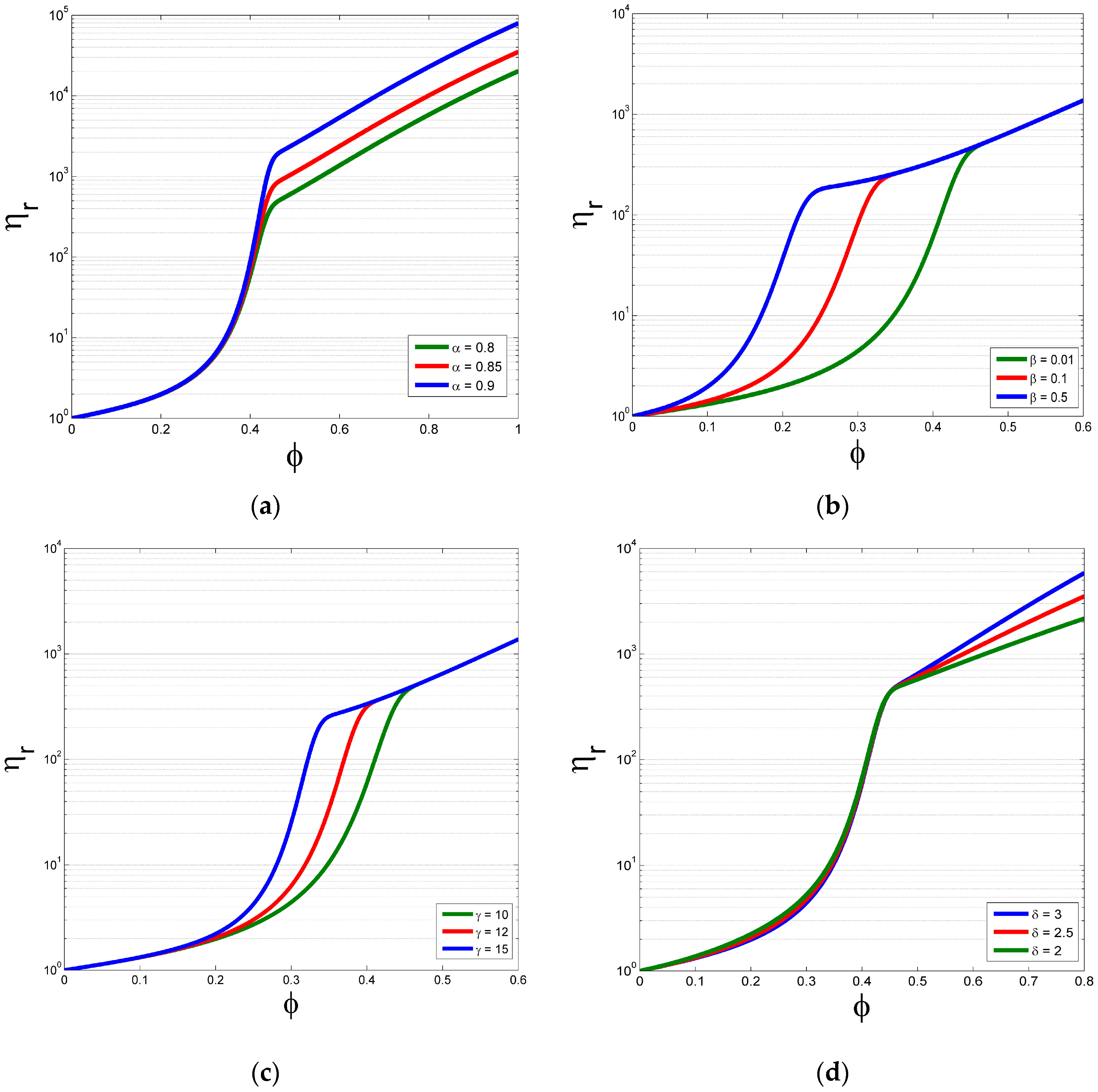
Figure 2.
Cumulative particle-size distribution for the kaolinite sample.
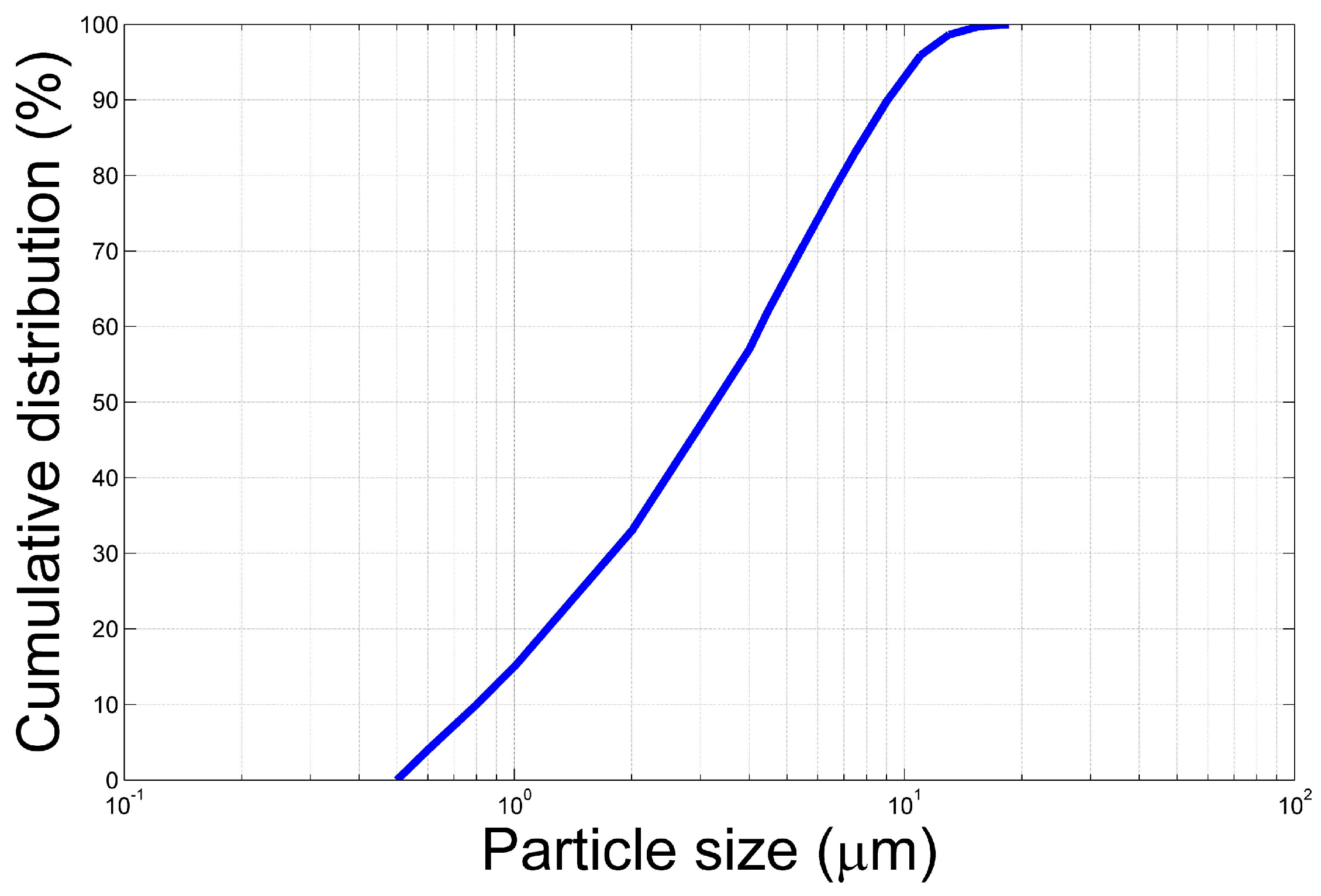
Figure 3.
Measured relative viscosity values as a function of kaolinite particle concentration.

Figure 4.
Comparison of measured data with the proposed equation, and other published formulae, including the Einstein equation [30], the Batchelor formula [31], the Roscoe formula [32], the Krieger and Dougherty formula [21], the Chong formula [22], the Dabak formula [23], the Liu formula [24] and the Boyer formula [25]. is taken as 0.48 in this study. Fitting values are: = 0.8, = 0.0096, = 10.3, and = 3.
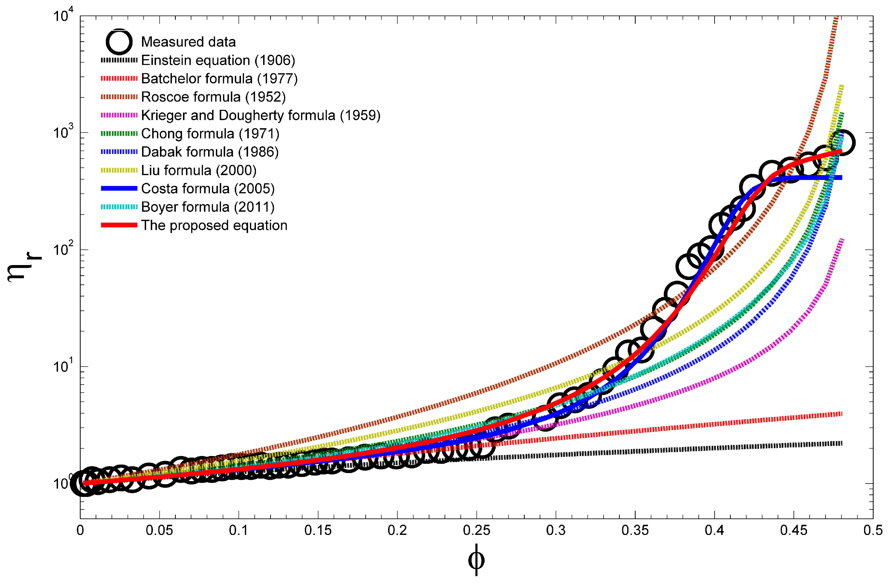
Figure 5.
Comparison of measured values (indicated by black circles) for the viscosity-crystal fraction relationship for partially crystallized Li2Si2O5 melt from Lejeune and Richet [37], predicted values from the proposed equation (indicated by red dashed line) and those from the Costa formula (indicated by blue dashed line). Here is taken as 0.45 from the experiment results of Lejeune and Richet [37]. The experimental temperature is 770.8 K. Fitting values of the proposed formula are: = 0.38, = 0.00001, = 20, and = 1.3.

Figure 6.
Comparison of measured data for the viscosity-crystal fraction relationship for partially crystallized Li2Si2O5 melt from Lejeune and Richet [37] with some published formulae, including the Einstein equation [30], the Batchelor formula [31], the Roscoe formula [32], the Krieger and Dougherty formula [21], the Chong formula [22], the Dabak formula [23], the Liu formula [24] and the Boyer formula [25]. Here is taken as 0.67 in this study.

Figure 7.
Comparison of measured viscosity-solid fraction values for partially melted granite (indicated by blue circle) from van der Molen and Paterson [36], partially crystallized Mg3Al2Si3O12 melt (green circle) from Lejeune and Richet [37], uniform spherical particles (red circle) from Thomas [42] at low solid concentration, and predicted values from the proposed equation (black dashed line) and those from the Costa formula (pink dashed line). Here is taken as 0.72 from the experiment results of van der Molen and Paterson [36], Lejeune and Richet [37] and Thomas [42]. The experimental temperature in Lejeune and Richet [37] is 1175 K. Fitting values of the proposed equation are: = 0.9975, = 0.014, = 3.5 and = 6.

Figure 8.
Comparison of measured viscosity-solid fraction values presented in Figure 7 and other published formulae, including the Einstein equation [30], the Batchelor formula [31], the Roscoe formula [32], the Krieger and Dougherty formula [21], the Chong formula [22], the Dabak formula [23], the Liu formula [24] and the Boyer formula [25]. Here is taken as 0.95.


Table 1.
Goodness of fit for the proposed equation, Costa formula and other published formulae (compared with measured data in Figure 3).
Table 1.
Goodness of fit for the proposed equation, Costa formula and other published formulae (compared with measured data in Figure 3).
| The Proposed Equation | Einstein Equation | Batchelor Formula | Roscoe Formula | Krieger and Dougherty Formula | Chong Formula | Dabak Formula | Liu Formula | Costa Formula | Boyer Formula | |
|---|---|---|---|---|---|---|---|---|---|---|
| R2 | 0.98 | 0.40 | 0.51 | 0.45 | 0.73 | 0.53 | 0.53 | 0.52 | 0.93 | 0.59 |
| NRMSE | 0.03 | 0.22 | 0.22 | 2.82 | 0.20 | 0.17 | 0.15 | 0.30 | 0.08 | 0.14 |
Table 2.
Goodness of fit for some published formulae (compared with published measured data in Figure 5).
Table 2.
Goodness of fit for some published formulae (compared with published measured data in Figure 5).
| Einstein Equation | Batchelor Formula | Roscoe Formula | Krieger and Dougherty Formula | Chong Formula | Dabak Formula | Liu Formula | Boyer Formula | |
|---|---|---|---|---|---|---|---|---|
| R2 | 0.85 | 0.94 | 0.71 | 0.71 | 0.71 | 0.71 | 0.71 | 0.71 |
| NRMSE | 0.46 | 0.45 | 130.40 | 4.07 | 8.60 | 11.11 | 12.99 | 5.16 |
Table 3.
Goodness of fit for published formulae based on the comparison with measured viscosity-solid fraction values presented in Figure 7.
Table 3.
Goodness of fit for published formulae based on the comparison with measured viscosity-solid fraction values presented in Figure 7.
| Einstein Equation | Batchelor Formula | Roscoe Formula | Krieger and Dougherty Formula | Chong Formula | Dabak Formula | Liu Formula | Boyer Formula | |
|---|---|---|---|---|---|---|---|---|
| R2 | 0.37 | 0.48 | 0.83 | 0.83 | 0.83 | 0.83 | 0.83 | 0.83 |
| NRMSE | 0.26 | 0.26 | 0.28 | 0.12 | 0.25 | 0.25 | 0.25 | 0.26 |
© 2017 by the authors. Licensee MDPI, Basel, Switzerland. This article is an open access article distributed under the terms and conditions of the Creative Commons Attribution (CC BY) license (http://creativecommons.org/licenses/by/4.0/).
Share and Cite
MDPI and ACS Style
Zhu, Z.; Wang, H.; Peng, D. Dependence of Sediment Suspension Viscosity on Solid Concentration: A Simple General Equation. Water 2017, 9, 474. https://doi.org/10.3390/w9070474
AMA Style
Zhu Z, Wang H, Peng D. Dependence of Sediment Suspension Viscosity on Solid Concentration: A Simple General Equation. Water. 2017; 9(7):474. https://doi.org/10.3390/w9070474
Chicago/Turabian StyleZhu, Zhongfan, Hongrui Wang, and Dingzhi Peng. 2017. "Dependence of Sediment Suspension Viscosity on Solid Concentration: A Simple General Equation" Water 9, no. 7: 474. https://doi.org/10.3390/w9070474
Note that from the first issue of 2016, this journal uses article numbers instead of page numbers. See further details here.