Assessing the Effects of Climate Change on Water Quantity and Quality in an Urban Watershed Using a Calibrated Stormwater Model

Abstract

Assessing climate change (CC) impacts on urban watersheds is difficult due to differences in model spatial and temporal scales, making prediction of hydrologic restoration a challenge. A methodology was developed using an autocalibration tool to calibrate a previously developed Storm Water Management Model (SWMM) of Difficult Run in Fairfax, Virginia. Calibration was assisted by use of multi-objective optimization. Results showed a good agreement between simulated and observed data. Simulations of CC for the 2041–2068 period were developed using dynamically downscaled North American Regional CC Assessment Program models. Washoff loads were used to simulate water quality, and a method was developed to estimate treatment performed in stormwater control measures (SCMs) to assess water quality impacts from CC. CC simulations indicated that annual runoff volume would increase by 6.5%, while total suspended solids, total nitrogen, and total phosphorus would increase by 7.6%, 7.1%, and 8.1%, respectively. The simulations also indicated that within season variability would increase by a larger percentage. Treatment practices (e.g., bioswale) that were intended to mitigate the negative effects of urban development will need to deal with additional runoff volumes and nutrient loads from CC to achieve the required water quality goals.

1. Introduction

Historical evaluations of the U.S. climate (1950–2009) revealed significant temperature increases for nearly all US cities, which was attributed to climate change (CC) as opposed to “heat island” effects caused by urban development [1]. Nearly 30% of the urban areas exhibited a significant increase in extreme precipitation. Hayhoe et al. [2] predicted an increase in precipitation during winter and spring under higher and lower emissions by the end of the 21st century. Najjar et al. [3] found that, in the mid-Atlantic region, precipitation magnitude and intensity, CO₂ concentrations, sea level, and water temperatures are likely to increase by the end of the 21st century. These predicted increases in rainfall magnitude and intensity could cause infrastructure failures due to increased runoff volumes and rates [4,5,6,7], overwhelming systems designed for much less. Limited studies using design storms and intensity-duration-frequency (IDF) curves have been conducted to assess the relative impact of CC on stormwater infrastructure. For example, Madsen and Figdor [8] found that CC in the mid-Atlantic region would increase the frequency of a one-year return period storm to 7.7 months. Moglen and Rios Vidal [9] used intensity-duration-frequency (IDF) curves generated from regional climate models (RCMs) to assess impacts from urban development and CC and concluded that the impact on infrastructure from each was roughly equivalent. Peck et al. [10] used a non-parametric weather generator to develop IDF curves for CC scenarios and found significant increases in anticipated precipitation intensities. Collectively, these studies provide a first assessment of what could be a major impact of CC, increased flooding of urban areas, which will require significant efforts, both financial and regulatory, to address [11].

More complex methods have been conducted using continuous simulation modeling incorporating altered climate predictions produced by a global climate model (GCM) and/or RCMs. Unfortunately, GCMs lack the spatial and temporal resolution for application to urban watersheds, and while the spatial resolution of RCMs (50 km²) is acceptable, they cannot achieve the sub-hourly temporal scales necessary to simulate the flashy urban runoff response [12]. Downscaling is a method used to bridge the mismatch between the spatial resolution of GCMs and RCMs and the required resolution for assessment of the CC impacts [13]. Two widely used downscaling methods are dynamical and statistical downscaling. Systematic errors are inevitable in RCM outputs; therefore, bias correction is often necessary after downscaling to a higher spatial resolution. Biases may occur in the climate model outputs due to a coarse spatial resolution, simplified processes, or numerical diffusion inherent in any model. Such errors can affect the projected results and should be corrected before using any climate model [14]. Wood et al. [15] reviewed six methods for generating future precipitation data for use in runoff modeling, consisting of three statistical downscaling methods: linear interpolation (LI), spatial disaggregation (SD), and bias-correction and spatial disaggregation (BCSD) applied to either the Parallel Climate Model GCM (PCM) or to the output after using a RCM to downscale the PCM. The authors found that the BCSD applied to the dynamically downscaled RCM was able to reproduce observed weather and provided the most plausible results compared to historical data. Teutschbein and Seibert [16] compared linear scaling, local intensity scaling, power transformation, variance scaling, distribution transfer, and the delta-change approach, and found that all methods were capable of correcting bias; however, significant differences were apparent between them. Gudmundsson et al. [17] compared distribution derived, parametric, and nonparametric transformation methods for correcting bias of RCM outputs. The results indicated that nonparametric transformations were best at reducing bias in RCM outputs. Lafon et al. [18] compared linear, nonlinear, γ-based quantile mapping, and empirical quantile mapping for reducing bias in RCM precipitation output. The results revealed that the third (skewness) and fourth (kurtosis) moments were sensitive to the choice of bias correction method, and the γ-based quantile-mapping technique performed significantly better than other methods. Linear scaling, local intensity scaling, daily translation, daily bias correction, quantile mapping based on an empirical distribution, and quantile mapping based on a gamma distribution were compared by Chen et al. [14] to reduce bias from RCM outputs driven by North American Regional CC Assessment Program (NARCCAP) data. The results indicated all methods improved RCM output. Chen et al. found the calibration performance of a hydrological model was influenced by bias correction method and watershed location.

Rosenberg et al. [19] compared historical hourly precipitation data sets from Washington State from 1970 to 2000 to a generated dynamically downscaled data set from 2020 to 2050 and output from a weather generator from several GCMs, and used these data to estimate streamflow. While few areas showed statistically significant differences in streamflow, the authors caution that improvements in downscaling methods for RCM outputs need to be made before results could be generalized sufficiently for drainage design. Recently, Wang and Chen [20] developed and tested a bias correction method using a modified version of equiratio cumulative distribution function matching. This method corrects model data using multiplicative scaling factors and improves the equidistant approach in bias correction of precipitation and enhances its performance. A modified version of this method was used for downscaling RCMs in this paper.

A variety of models are available for simulation of runoff, including Win TR-55 [21], Hydrologic Engineering Center Hydrologic Modeling System (HEC-HMS) [22], Mike-Urban [23], and the U.S. Environmental Protection Agency’s (EPA) Storm Water Management Model (SWMM) [24,25]. HEC-HMS, Mike-Urban, and SWMM have the capability of being used in both event-based and continuous simulation modes [26,27]. Of these three, HEC-HMS and SWMM are in the public domain. SWMM is widely applied for continuous rainfall-runoff simulation in urban areas [28,29,30]. SWMM simulates surface runoff, infiltration, evapotranspiration (ET), snowmelt, surface water routing, surface water storage, groundwater, water quality, and treatment processes. SWMM is able to simulate the production of pollutant loads associated with runoff through modeling buildup and washoff processes from specific land uses during dry weather and storm events, respectively [31].

Urban development creates large amounts of impervious surfaces for roads, parking, buildings, and sidewalks. As impervious surfaces are created, large increases in runoff volume and rates occur. SWMM has been applied to evaluate the combined hydrologic impacts of urbanization and CC [28,32,33,34]. Few studies were found addressing water quality impacts from CC in urban areas at the watershed scale. Hydrologic changes from urban development cause erosion from landscapes and streambanks, as well as channel scour and degradation [35,36]. Runoff mobilizes pollutants such as metals, nutrients, and toxicants [37], affecting streams, lakes, rivers, and estuaries as runoff is transported downstream. Elevated nutrient levels contribute to aquatic “dead zones” affecting many estuaries worldwide, perhaps the most notable example being the Chesapeake Bay [38]. To address deterioration of the aquatic health of the Bay, the U.S. EPA established a Total Maximum Daily Load (TMDL), restricting nitrogen (N), phosphorus (P), and sediment in discharges to each tributary of the Chesapeake Bay [39]. The objective of the TMDL is to reduce N, P, and sediment loadings by implementing stormwater control measures (SCMs), also known as best management practices (BMPs), to reduce runoff or N, or P, and/or sediment loading. CC impacts temperature, precipitation, and other climatic variables (wind speed, humidity, solar radiation, and etc.) [40,41], leading to changes, often reductions in SCM effectiveness [42]. N, P, and sediment export from the landscape to surface waters are controlled by the combination of key biogeochemical processes driven by hydrologic transport. When the potential impact of CC variability is added to the system, critical biogeochemical processes will be altered across the Chesapeake Bay watershed [43]. A better understanding of these coupled processes is critical to managing N, P and sediment exports from the Bay watershed to the estuary from urban and agricultural systems; this paper focuses on the urban contribution to watershed loading for N, P, and sediment. Improving the ability to predict CC impacts on water quality in urban watershed is needed to evaluate conditions and select the best treatment options.

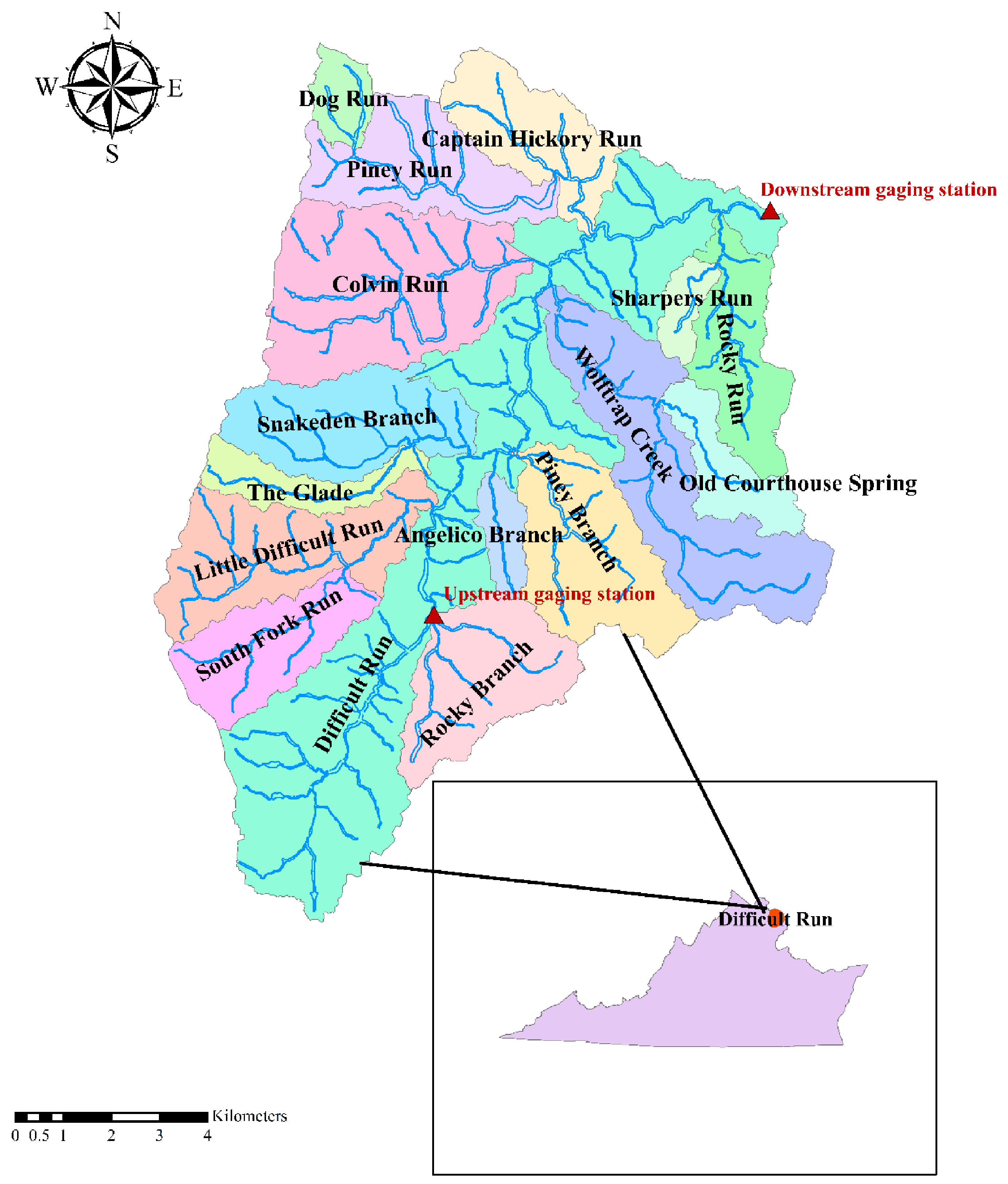
The objective of this study is to evaluate the impacts of CC on an urban watershed including the impact on runoff volume, peak flow, and water quality (Total Suspended Solids, TSS; Total Nitrogen, TN; and Total Phosphorous, TP), using a SWMM calibrated with a robust autocalibration tool, R for Storm Water Management Model (RSWMM), developed within the R environment. Hourly precipitation data from a mid-range emission scenario and regional climate model are used to force the SWMM model. A multi-objective optimization package, the Non-dominated Sorting Genetic algorithm (NSGA-II) was incorporated into RSWMM, providing functions for box-constrained multi-objective optimization using a genetic algorithm. A postprocessor for classifying output into events and plotting probability of exceedance curves of user selected outputs was incorporated for ease of comparing scenarios. As a case study, the tool is applied to the calibration of a previously developed SWMM model of the Difficult Run watershed in Fairfax County, Virginia, which is tributary to the Chesapeake Bay, using historical and downscaled projected precipitation and temperature data. This new and novel method will then be used to assess the impact of CC on predicted water quality from the watershed.

2. Methods

2.1. Study Area

The Difficult Run watershed, the largest watershed in Fairfax County VA, is 150 km² in size, and consists of 18 named tributary sub-watersheds (Figure 1). The Difficult Run mainstem is approximately 63 km in length, and the length of its tributaries is approximately 233 km. Ground slope is low to moderate. The watershed is within Piedmont physiographic province of Virginia and is part of the greater Washington, D.C., metropolitan region.

Soils are classified by NRCS into four soil hydrologic groups ranging from A to D, where A has the least runoff potential and D has the greatest runoff potential. The majority of the soils in the watershed (40.5%) are Glenelg, soil hydrologic group B, which signifies a moderate infiltration capacity, but is also highly susceptible to erosion [44]. A small proportion (5%) of the soils adjacent to streambeds are subject to inundation during high flows. Current land uses in the Difficult Run watershed range from forest to urban; of the latter, the most predominant subtype is urban residential development at approximately 57% [44]; shown in

Table 1. Existing landuse/landcover Difficult Run watershed.

LULC Type	Existing (%)
Open Water	0.4
Developed, Open Space	32.2
Developed, Low Intensity	12.5
Developed, Medium Intensity	6.6
Developed, High Intensity	1.47
Barren Land (Rock/Sand/Clay)	0.02
Deciduous Forest	35.9
Evergreen Forest	2.11
Mixed Forest	1.39
Shrub/Scrub	0.9
Grassland/Herbaceous	0.06
Pasture/Hay	1
Cultivated Crops	0.8
Woody Wetlands	4.3
Emergent Herbaceous Wetlands	0.01

. The percentage of impervious surfaces in the watershed is approximately 18.4%, which is about 1/3rd of the urban area [44].

Like much of Fairfax County and metropolitan D.C., the Difficult Run watershed has experienced significant urban development, which has degraded water quality, reduced aquatic habitat, and increased flooding not unlike other streams draining rapidly urbanized watersheds [45]. After conducting a detailed hydrologic and water quality study of the Difficult Run watershed, a comprehensive watershed management plan (WMP) was adopted by Fairfax County Fairfax County [44] to address water quality and quantity issues. In the development of the WMP, over 900 existing SCMs were assessed. These SCMs provide peak flow storage and varying degrees of treatment for urban runoff. The WMP assessed stream conditions for the mainstem and 18 main tributaries. Using geographic information system (GIS) data provided by the county, hydraulic/hydrologic (H/H) and water quality models were developed for the Difficult Run watershed [44]. These models were used to assess current conditions, and to guide future management planning to meet water quantity and quality goals under anticipated future conditions.

After the study was complete, the U.S. Geological Survey (USGS), in partnership with Fairfax County, conducted a comprehensive, seven-year monitoring program of Difficult Run [46]. This study provided the hydrologic and water quality data used for calibration and verification. Difficult Run sediment yields ranged from 378.3 to 9939.2 kg per ha (kg/ha) annually; with higher loads associated with the degree of urbanization. Total N loads ranged from 4.1 to 18.2 metric tons and corresponding yields ranged from 5.9 to 14.7 kg per ha (kg/ha), annually. Total P loads ranged from 0.190 to 3.79 tones and corresponding yields ranged from 0.24 to 2.8 kg per ha (kg/ha), annually. Monitoring stations in Difficult Run showed higher TSS loading in 2008, and 2011 associated with Tropical Storms Hanna and Lee, respectively. Dissolved N composed 60 to 85 percent of the total annual N load, and the annual dissolved N load was correlated with runoff volume [46]. Total P loads were composed of about 74% sediment-associated P, resulting in a strong correlation between total and dissolved P and annual peak runoff. Dissolved TN and TP sources in Difficult Run were attributed to application of fertilizer to residential lawns, and human and animal waste from inefficient septic systems [46].

2.2. Hydraulic/Hydrology (H/H) Modeling

Urban H/H models use climatological data (precipitation, temperature), land use data, and hydraulic system data to estimate water and pollutant flux across the landscape by simulating hydrologic and water quality processes. Key hydrologic processes include rainfall-runoff, infiltration, evapotranspiration, and flow routing. In this study, the U.S. EPA’s SWMM version 5.1.010 was employed for H/H modeling (U.S. Environmental Protection Agency, Edison, NJ, USA). SWMM can perform both single event and continuous simulation and has been widely used in urban areas [24,25,31,47]. Outputs of the model include runoff and/or streamflow and water quality constituent loads and/or concentrations. SWMM simulates groundwater flow for each subcatchment through a single aquifer, which is defined by the depth of its unsaturated upper zone and lower saturated zone, bottom of aquifer, groundwater flow parameters, porosity, wilting point, field capacity and saturated hydraulic conductivity. This data was obtained from the geologic map [48,49] and SSURGO database [50]. These parameters were taken from raster grids or attributes associated with a specific area. GIS spatial operations were conducted to create a weighted area average for each subcatchment.

Evaporation from subcatchment surfaces, from subsurface water in aquifers, and from streams was modeled using methods outlined in [51]. SWMM uses the Hargreaves equation for evaporation simulation [31]. Evaporation in the SWMM models used in this study was computed from daily minimum and maximum temperatures, including historical or projected. The Green-Ampt infiltration method was used to estimate infiltration and excess rainfall. This method was selected due to the physical basis of its parameters (suction head, hydraulic conductivity, and initial moisture deficit), and their availability in the Soil Survey Geographic database (SSURGO) database [50]. Flow routing used SWMM’s dynamic wave option was selected due to its accuracy and ability to simulate non-uniform, unsteady state flow conditions. Land use and soil data for the watershed were obtained from the WMP [44]. Two USGS stream gauges draining areas of 7 km² and 150 km², respectively, are located within the watershed. Data from these stations were used to calibrate and verify the model. Then, projections for precipitation, and temperature across the watershed from the NARCCAP [52] for historical and future conditions was used in the calibrated and verified model to predict streamflow, and TSS, TN and TP concentrations for historical and projected CC conditions.

2.3. Water Quality Modeling

Water quality was modeled using an estimated event mean concentration (EMC) washoff loading during runoff events. A simple treatment functions which is commonly used in many urban models were employed in this study as follows:

$$C_{t+1}=C_0(1-e^{-kt})$$

(1)

where: $C_{t+1}$ is concentration of pollutant at time t + 1 in mg/L, $C_0$ is initial concentration of pollutant in mg/L, and k is removal constant.

Water quality characteristics were developed based upon EMCs, which were set to 40 mg/L for TSS, 2.9 mg/L for TN, and 0.27 mg/L for TP, based upon average values for Virginia [53].

In SWMM, water quality treatment expressions have the form of:

$$R=\{P,R_P,V\}$$

(2)

$$C=\{P,R_P,V\}$$

(3)

where: R is fractional removal, C is concentration of pollutant in mg/L, P is the pollutant, R_p is the pollutant removal for pollutant, and V is a process variable.

Treatment expressions in SWMM were developed by assuming irreducible concentrations [54]. This concept holds that treatment effectiveness is reduced once a low level of pollutant concentration has been reached, i.e., it gets more difficult to remove the last fraction of pollutant. The irreducible concentration relationship is often used to characterize runoff quality data [55], and was recently applied by Chretien et al. to characterize TSS, TN, and TP behavior within an agricultural BMP [56]. TSS and TN concentrations were estimated by:

$$C_{\mathrm{TSS},i+1}=20+(C_{\mathrm{TSS},i}-20)e^{-{10}^{-4}(\frac{\mathrm{DT}}{D})}$$

(4)

$$C_{\mathrm{TN},i+1}=1.9+(C_{\mathrm{TN},i}-1.9)e^{-0.5·{10}^{-9}(\frac{\mathrm{DT}}{D})}$$

(5)

where: $C_{TSS}$ is the concentration of TSS, and $C_{TN}$ is the concentration of TN, D is water depth in m, DT is time step in seconds, i and i + 1 represent the previous and current time.

TP was split into two fractions, soluble phosphorus (SP) and particulate phosphorus (PP):

$$C_{\mathrm{TP},i+1}=C_{\mathrm{SP},i+1}+C_{\mathrm{PP},i+1}$$

(6)

The SP reduction was estimated by:

$$C_{\mathrm{SP},i+1}=0.23+(C_{\mathrm{SP},i}-0.23)e^{-5.2·{10}^{-5}(\frac{\mathrm{DT}}{D})}$$

(7)

The PP reduction was computed as a function of removal of TSS:

$$R{R}_{\mathrm{PP}}=R_{\mathrm{TSS}}$$

(8)

2.4. R for Stormwater Management Model (RSWMM)

In order to efficiently calibrate the model without altering the SWMM source code, an external, freely available control program was needed. SWMM is constantly being updated; so, use of a non-altered SWMM source code ensures compatibility with future updates. R [57] (RCD Team, 2015) is an open source, freely available system that can be used for statistical analysis and programming. R has been successfully used in hydrological modeling and its capabilities are well recognized [58]. R is compatible with most operating systems. Because of these capabilities, R was chosen for use in this study for development of a control module that could execute SWMM simulations repetitively, changing key parameters according to user needs. An existing R code known as RSWMM (https://www.openswmm.org/Topic/4390/rswmm-autocalibration-of-swmm-in-r) was identified and was used for this study [59]. Several enhancements were developed as part of this project, including separation of events, incorporating an autocalibration tool described in a later section, and a post-processor to view exceedance curves of the output. The reader is referred to

Table A1. Software/Data Availability.

Software/Data Availability	Information
Name of software or data set	RSWMM
Developer and contact address	Peter Steinberg (original), Nasrin Alamdari (this revised version)
Telephone	216-715-4492; 716-239-9288
Fax	(540) 231-3199
Email numbers	[email protected]; [email protected]
Year first available	3/24/2014
Hardware required	Personal computer, recommended minimum 64 bit machine, i7 or better, 8GB RAM or better, at least 500 GB storage available
Software required	R 3.2.5 for windows available for free download from https://cran.r-project.org/bin/windows/base/
Availability	https://github.com/RSWMM/R--Stormwater-Management-Model
Cost	Free
Program language	R
Program size	76 kb
Data: form of repository (database, files, spreadsheet)	Files
Size of archive	<1 MB
Access form	FTP

in the Appendix A for further information on the RSWMM code.

2.5. Calibration

A typical SWMM model application contains many input parameters. As mentioned previously, SWMM model outputs are sensitive to hydraulic width, imperviousness and depression storage depth [34,60], the first two parameters being positively correlated to peak flow, the latter, negatively correlated. Calibration of the Difficult Run watershed model was conducted by varying hydraulic width (the sub-catchment area divided by the maximum overland flow length), imperviousness and depression storage depth (a depth that must be filled prior to the runoff occurs) for 2010 data. Hourly rainfall data were disaggregated to 15-min time step for the proposed H/H simulations using NETSTORM [61]. Then, the simulation results were aggregated to an hourly time series and SWMM was calibrated with respect to peak flows and runoff volume during all events in upstream and downstream catchments. A 6 h minimum inter-event period was used to classify data into events. Two gauging stations located in upstream and downstream sub-watersheds (location shown in Figure 1) were used for calibration and verification. Calibration and verification were performed using events from 2010 and 2013, to calibrate and verify the model performance, respectively.

2.6. Autocalibration Methods

The autocalibration tool within RSWMM utilizes a multi-objective optimization package, NSGA-II, which provides functions for box-constrained multi-objective optimization. Three objective functions were used. These included: coefficient of determination (R²), Nash Sutcliffe Efficiency (NSE), and Percent Bias (PBIAS). R² describe the degree of collinearity between simulated and observed data and ranges from 0 to 1. R² close to 1 indicate less error variance and is desirable. Values greater than 0.5 are considered satisfactory in the study by Santhi et al. [62] and Van Liew et al. [63].

NSE is a normalized statistic which indicates how well the plot of observed versus simulated data fits and ranges from −∞ to 1.0 [64]. A value of NSE close to 1 is considered as an excellent level of performance. NSE was calculated as:

$$\mathrm{NSE}=1-\left[\frac{{{\displaystyle \sum }}_{i=1}^{i=n}{({Y_i}^{obs}-{Y_i}^{sim})}^2}{{{\displaystyle \sum }}_{i=1}^{i=n}{({Y_i}^{obs}-Y^{mean})}^2}\right]$$

(9)

where ${Y_i}^{obs}$ is observed data values, ${Y_i}^{sim}$ is simulated data values, and $Y^{mean}$ is the mean of observed data.

Percent bias (PBIAS) shows the deviation of data and expressed as a percentage. It measures the average tendency of the simulated data to be different from observed data [65]. PBIAS close to 0 is considered to be an excellent level of performance. PBIAS was calculated as:

$$\mathrm{PBIAS}=\left[\frac{{{\displaystyle \sum }}_{i=1}^{i=n}({Y_i}^{obs}-{Y_i}^{sim})\times 100}{{{\displaystyle \sum }}_{i=1}^{i=n}({Y_i}^{obs})}\right]$$

(10)

where ${Y_i}^{obs}$ is observed data values, and ${Y_i}^{sim}$ is simulated data values.

SWMM was calibrated using an autocalibration procedure, adjusting specific model parameters described within a defined range. Observed and simulated outputs were compared at upstream and downstream gauging stations to determine the parameter set that provide the best model simulated runoff peak and volume. With the completion of a given optimization, sets of calibrated parameters were obtained through optimization. Default values that were used from the previously developed model as initial model parameters. Based on the study by Ref. [62,63], R² and NSE ≥ 0.75 and PBIAS ≤ ±10%, which are considered to be very good calibration performance. R² and NSE ≥ 0.65 and ±10% ≤ PBIAS ≤ ±15%, which are considered to be good calibration performance. R² and NSE ≥ 0. 5 and ±15% ≤ PBIAS ≤ ±20% are considered as satisfactory calibration performance. The autocalibration approach aims to minimize the difference between measured and simulated values. Initial parameter values were allowed to vary by ±20% to create parameter sets to initialize the autocalibration procedure. Calibration and verification were performed on the 2010 and 2013 data, respectively, with a maximum number of iterations set at 500. Because the SWMM model was based on subhourly rainfall data, the run time for each iteration was large.

2.7. Climate Modeling

To predict future CC impacts on runoff quantity and quality, projections are required for precipitation and temperature across the watershed. In this study, simulations from the North American Regional CC assessment program (NARCCAP) [52] were used. Projections were based upon dynamical downscaling; embedding a regional climate model (RCM) with 50 km² spatial resolution into a global climate model (GCM). Two time periods, 1971–1998 and 2041–2068 were used for historical and future CC conditions, respectively. The latter scenario represents a medium-high greenhouse gas emissions assumption, A2 [66].

Data were obtained from one GCM-RCM combination, the MM5I-CCSM, which was selected based on its ability to accurately simulate historical temperature and precipitation. Annual mean temperature and precipitation were averaged over the region for nine of the NARCCAP models including CRCM_cgcm3, ECP2_gfdl, HRM3_gfdl, HRM3_hadcm3, MM5I-CCSM, MM5I_hadcm3, RCM3_cgcm3, RCM3_gfdl, WRFG_cgcm3, and compared the means to the mean obtained from an observation-based dataset. Figure 2a,b show the annual mean temperature and precipitation of 9 models, respectively.

Although the historical performance of the model was reasonable, bias was still evident, so, bias-correction was conducted. Bias correction was applied using a modified version of the equiratio cumulative distribution function matching method [20]. This method corrects model data using multiplicative scaling factors. The scaling factor applied to each model data point is the ratio of the observed value at the data point’s quantile to the historical-period model value at the data point’s quantile. Using the notation of Wang and Chen [20], this is expressed mathematically as:

$${\tilde{x}}_{m-p,adjust}=x_{m-p}\times \frac{F_{o-c}^{-1}(F_{m-p}(x_{m-p}))}{F_{m-c}^{-1}(F_{m-p}(x_{m-p}))}$$

(11)

where $x_{m-p}$ is a value from the model during the prediction period (which may be either the historical or future period), $F_{m-p}$ is the empirical cumulative distribution function (CDF) of the model prediction data, $F_{o-c}^{-1}$ is the inverse CDF of the observed data, and $F_{m-c}^{-1}$ is the inverse CDF of the model data during the historical (or current) period. This correction method was applied to the model-simulated precipitation and temperature data for both time periods. The observed CDFs in the numerator of Equation (10) were determined using forcing data from Phase 2 of the North American Land Data Assimilation System (NLDAS-2) [67]. This dataset was selected since it has matching variables for all climate model data, it has a relatively high spatial (1/8 degree) and temporal (hourly) resolution, and did not have missing data.

Several modifications were applied to the correction algorithm. For precipitation, use of Equation (10) would set the frequency of zero precipitation to be equal to the observed frequency in the historical and future periods. To relax this restriction, model data with a CDF value less than the frequency of no precipitation in the observed dataset were set to zero. For the historical period, this results in the frequency of corrected model dry values equaling the frequency of observed dry values. However, for the future period the frequency of dry values in the corrected data may change. The correction in Equation (10) was then applied using only values greater than zero in each dataset. For downwelling shortwave radiation, the bias correction was only applied using modeled and observed values greater than zero. Model air temperature predictions were corrected using an additive shift rather than a multiplicative ratio. Unlike precipitation and other variables, an additive correction applied to temperature is unlikely to produce values that are below zero. The bias correction and temporal disaggregation were applied separately for each calendar month.

NARCCAP provides model output at three-hour intervals. This temporal resolution was deemed sufficient for all variables except precipitation. Temporal disaggregation was applied to convert precipitation data to hourly frequency using a method developed to create input data for the Variable Infiltration Capacity model [68]. This method starts with daily precipitation totals (produced from upscaled and subsequently bias-corrected 3 h NARCCAP precipitation) and uses a CDF mapping approach to assign the daily amounts to fall during hours such that the disaggregated model CDFs of precipitation duration and hour of occurrence match the observed CDFs, using hourly precipitation totals at the Ronald Reagan National Airport in Washington, D.C. Separate CDFs and corrections were applied for each calendar month and for five daily-total precipitation bins: 0–5, 5–10, 10–15, 15–20, and 20+ mm. Unlike the bias correction method, this temporal disaggregation method does not allow the distributions of duration and time of occurrence to change from the historical to the future period. However, because the disaggregation step preserves the daily total amounts, which it receives from the bias correction step, the daily total precipitation amounts may still change from the historical to the future CC projection.

2.8. Statistical Analysis

Changes in precipitation, runoff, TSS, TN, and TP in the watershed were investigated using the student’s t-test to find whether there was a significant difference between the historical and future conditions. The two-sample t-test was used to test the null hypothesis that the population means of two groups are the same. The t-test assumes the underlying distribution is normal, therefore the normality of the datasets was tested using Shapiro-Wilk test [69]. In addition, flow statistics, i.e., Q95, Q50 and Q10, which represent low, median, and high flows, respectively, were computed and compared to historical and predicted conditions using exceedance probability plots.

3. Results and Discussion

3.1. Calibration and Verification

Calibration and verification were performed using the data from upstream and downstream gauging stations. Performance metrics of the model with respect to peak flow and runoff volume after calibration and verification for upstream and downstream gauges are provided in

Table 2. Summary of model performance for calibration and verification periods at the Difficult Run upstream gauging station with respect to peak flow.

Period	Model Performance
	R2	NSE	PBIAS
Calibration	0.77	0.72	14.9%
Verification	0.83	0.79	13.8%

and

Table 3. Summary of model performance for calibration and verification periods at the Difficult Run downstream gauging station with respect to peak flow.

Period	Model Performance
	R2	NSE	PBIAS
Calibration	0.84	0.76	14.5%
Verification	0.78	0.73	12.1%

, respectively. According to the criteria of Santhi et al., Van Liew et al., and Moriasi et al. [62,63], and [70], simulated and observed runoff volume showed a good level of agreement on an event basis.

The most sensitive parameters identified in previous studies were hydraulic width, imperviousness, and depression storage for impervious and previous areas. During calibration, each parameter was adjusted to improve agreement between observed and predicted peak flows and runoff volume. However, adjusting the hydraulic width of some of the smaller catchments in the watershed did not have much impact on runoff. Depression storage for impervious and pervious did not have significant effects on the results. Calibration and verification results based on the peak flows are shown in Figure 3 and Figure 4.

The results indicate an underestimation of peak flow in the verification period, especially in wet events that may be due to missing of some processes in the SWMM model such as groundwater recharge. While SWMM has a groundwater flow component, it is primarily a surface runoff model, and some subsurface processes are neglected [31]. Flows that are produced via infiltration loss and routed through subsurface may not be fully captured and simulated by the model.

Performance metrics of the model with respect to runoff volume for upstream and downstream gauges are provided in

Table 4. Summary of model performance for calibration and verification periods at the Difficult Run upstream gauging station with respect to runoff volume.

Period	Model Performance
	R2	NSE	PBIAS
Calibration	0.74	0.71	−17.8%
Verification	0.75	0.65	6.1%

and

Table 5. Summary of model performance for calibration and verification periods at the Difficult Run downstream gauging station with respect to runoff volume.

Period	Model Performance
	R2	NSE	PBIAS
Calibration	0.78	0.73	13.3%
Verification	0.72	0.69	15.4%

, respectively. The results revealed that simulated and observed runoff volume showed a good level of agreement on an event basis.

Simulated and observed hydrographs for some selective events including dry and wet events are shown in Figure 5.

Average annual flow in the calibration and verification period at upstream and downstream gauging stations are provided in

Table 6. Annual mean flow of simulated and observed data at the Difficult Run upstream gauging station.

Period	Annual Flow (m3/s)
	Simulated	Observed
Calibration	0.34	0.26
Verification	0.29	0.23

and

Table 7. Annual mean flow of simulated and observed data at the Difficult Run downstream gauging station.

Period	Annual Flow (m3/s)
	Simulated	Observed
Calibration	1.81	2.01
Verification	1.76	1.67

, respectively. The results indicate good performance of the calibration in simulating mean annual flow during calibration and verification periods. A map of the model calibrated parameters by sub-catchments in the watershed are provided in Figure 6.

A simplified assessment of performance was conducted by comparing predicted values with station annual loads. Model results at the upstream gauging station for TSS, TN, and TP showed an R² of 0.61, 0.57, and 0.58, respectively, during the calibration; and an R² of 0.65, 0.59, and 0.61, during the calibration at the downstream gauging station. The performance of the model through calibration for TSS, TN, and TP is illustrated in Figure 7a,b for upstream and downstream gauge locations, respectively. The final model parameters for each sub-catchment are provided in

Table 8. Model calibrated parameters for sub-catchments in the Difficult Run watershed.

Sub Catchments	Model Parameters
	Hydraulic Width (m)	Imperviousness (%)	Depression Storage (Previous) (cm)	Depression Storage (Impervious) (cm)
Angelico Branch	667.8	7.4	0.51	0.3
Captain Hickory Run	674.1	7.7	0.58	0.31
Colvin Run	645.6	16.3	0.68	0.38
Difficult Run (Lower)	779.1	6.5	0.67	0.29
Difficult Run (Middle)	200.7	10.1	0.54	0.37
Difficult Run (Upper)	850.3	24.8	0.56	0.43
Dog Run	667.8	11.1	0.53	0.41
The Glade	699.6	11.3	0.61	0.33
Little Difficult Run	683.7	7.4	0.64	0.31
Old Courthouse Spring Branch	745.7	29.5	0.53	0.35
Piney Branch	689.1	16	0.56	0.32
Piney Run	604.2	11.4	0.56	0.27
Rocky Branch	689.1	12.2	0.61	0.38
Rocky Run	705.9	8.4	0.66	0.3
Sharpers Run	665.6	6.8	0.63	0.3
Snakeden Branch	711.7	19	0.69	0.27
South Fork Run	715.5	8.6	0.55	0.43
Wolftrap Creek	685.3	16.2	0.53	0.36

.

3.2. Climate Change Impacts

After calibration and verification, the flow and water quality in the watershed was simulated for the 2041–2068 period. The annual average flow and water quality during historical and future periods were calculated and compared. The simulation results indicate that the mean annual runoff is predicted to increase by 6.5% with CC. The mean annual TSS, TN, and TP were predicted to increase by 7.7%, 7.0%, and 8.1%, for upstream and downstream locations, respectively.

Seasonal changes in runoff, TSS, TN, and TP are shown in Figure 8a–c, respectively.

Annual precipitation for 2041–2068 increased by 6.1%, while temperature rose by 1.6 °C relative to 1971–1998. Seasonal changes in runoff during 2041–2068 ranged from −22.3% to 32.3%, with the highest increase occurring from October to December. Analysis of seasonal runoff variations indicates increasing runoff in fall and summer and decreasing in winter and spring. Smaller increases in runoff were predicted during the summer, which could be due to increased evapotranspiration and less groundwater recharge. In the CC projections, summer and fall are associated with more precipitation and higher temperatures, with more frequent occurrences of heavy precipitation. Higher temperatures will lead to higher evapotranspiration rates and lower soil moisture. Lower rainfall and higher temperatures in the winter and spring will result in less runoff volume because the water can be absorbed by the soil, whereas higher rainfall and temperature in summer and fall will lead to increased runoff volume due to more precipitation.

Precipitation during the CC projection was characterized by more frequent occurrences of heavy precipitation. Annual mean temperature during the CC projection was 1.6 °C warmer than during the historical period; the warming is relatively uniform throughout the seasons. During September–December, the model predicted runoff, TSS, TN, and TP to increase by 22.5%, 13.2%, 12.8%, and 14.1%, respectively, relative to the historic time period. On a monthly basis, the greatest expected increase was December, with runoff volume, TSS, TN, and TP projected to increase by 32.3%, 29.7%, 24.8%, and 37.7%, respectively. April shows the greatest decrease, with runoff volume, TSS, TN, and TP projected to decrease by 22.3%, 25.7%, 24.7%, and 27.3%, respectively. Imperviousness in highly urbanized watersheds like Difficult Run has been identified as one of the main drivers of runoff pollution and stream degradation [46] from this watershed. Increased precipitation resulting from CC would result in increased streamflow which will likely lead to further stream instability and erosion, resulting in further water quality degradation from anticipated higher level of imperviousness, temperature, and precipitation.

Pair-wise comparison to determine if there was a significant difference between the mean monthly historical and CC projections was conducted using a t-test for runoff volume, TSS, TN, and TP. A Shapiro-Wilk test [69] indicated that, at p-value > 0.05, the dataset follows a normal distribution. The results of t-test are shown in

Table 9. Student’s t-test pairwise results.

Simulation Results	Statistical Parameters
	t-Calculated	t-Critical	p-Value
Runoff Volume	0.27	2.2	0.78
TSS	1.64	2.2	0.12
TN	1.35	2.2	0.2
TP	3.63	2.2	0.003

.

The results of the t-test indicated that the differences between the mean monthly values of historical and predicted CC runoff volume, TSS, and TN were not significant at the 95% confidence level. TP values were significantly different at 95% confidence interval, which implies that TP may be more sensitive to CC. In general, TP loads are composed of soluble phosphorus (SP) and particulate phosphorus (PP), both of which are strongly correlated with TSS and peak runoff. As a result, increases in peak runoff and TSS may lead to higher levels of TP compared to runoff, TSS, and TN in the watershed under anticipated CC.

The mean, median, and maximum values, and the range between the 10th and 95th percentiles (Q10 and Q95) for the future period, were compared with statistical parameters for the historical period (

Table 10. Statistical parameters during events for the historical and future periods.

Simulation Results	Statistical Parameters
	Mean	Median	Max	Range (90th–10th)
Historical Period
Runoff Volume (m3)	4.5	0.8	100.3	26.91
TSS (mg/L)	186.4	154.2	859.4	510.4
TN (mg/L)	18	14.9	79.4	48.7
TP (mg/L)	0.29	0.0008	3.49	1.5
Future Period
Runoff Volume (m3)	10.4	1.32	166.2	53.9
TSS (mg/L)	221.7	167.1	1010	553.1
TN (mg/L)	21.2	15.89	93.8	53
TP (mg/L)	0.45	0.06	4.2	1.8

). Compared with the historical period, the mean, median, maximum runoff volume, TSS, TN, and TP loads during the events increase under CC.

In addition to the increase in the mean, median, maximum, runoff, TSS, TN, and TP, the interannual variability increased in most months. Interannual variability of precipitation, temperature, streamflow, TSS, TN, and TP are shown in Figure 9a–f, respectively.

To analyze the effect of CC on runoff volume and water quality parameters, exceedance probability curves were developed, as shown in Figure 10a–d, for runoff volume, TSS, TN, and TP, respectively. The curves were created by plotting the simulated results by event for the historical and future periods. Values of runoff volume, TSS, TN, and TP for the 10th, the 50th, and 95th percentiles are provided in

Table 11. Statistics during events for the historical and future periods.

Simulation Results	Statistical Parameters
	Q10	Q50	Q95
Historical Period
Runoff Volume (m3)	28.92	0.8	0.0012
TSS (mg/L)	529.36	154.2	15.4
TN (mg/L)	50.8	14.9	1.1
TP (mg/L)	1.61	0.0008	1.8 × 10−7
Future Period
Runoff Volume (m3)	55.95	1.32	0.0031
TSS (mg/L)	583.12	167.1	20.1
TN (mg/L)	55.9	15.89	1.9
TP (mg/L)	1.91	0.06	6.5 × 10−5

.

Figure 10a shows a significant difference between the historical and future runoff volume during larger storm events occurring at the 10% probability. Historical and future exceedance curves for TSS and TN track very closely, except for small differences apparent in mid-range events (Figure 10b,c). Of the water quality constituents, TP shows the most difference, and there are more frequent events (Figure 10d). Results in Table 11 show that all the flow statistics (Q95, Q50, and Q10) increase under CC. The results also indicate a 30% to 158% increase in Q10.

The results of this study provide a guidance to better understand which pollutants are most critical and pose the greatest variability under CC projections. Therefore, it helps managers and decisionmakers develop better mitigation actions and select the most appropriate SCMs. It may enable a more reliable and rational CC decision-making process for this specific case study watershed. Overlooking the impact of CC on water quantity and quality could result in failing to achieve water quality goals, may result in unanticipated flooding, and likely will result in damages and waste.

4. Conclusions

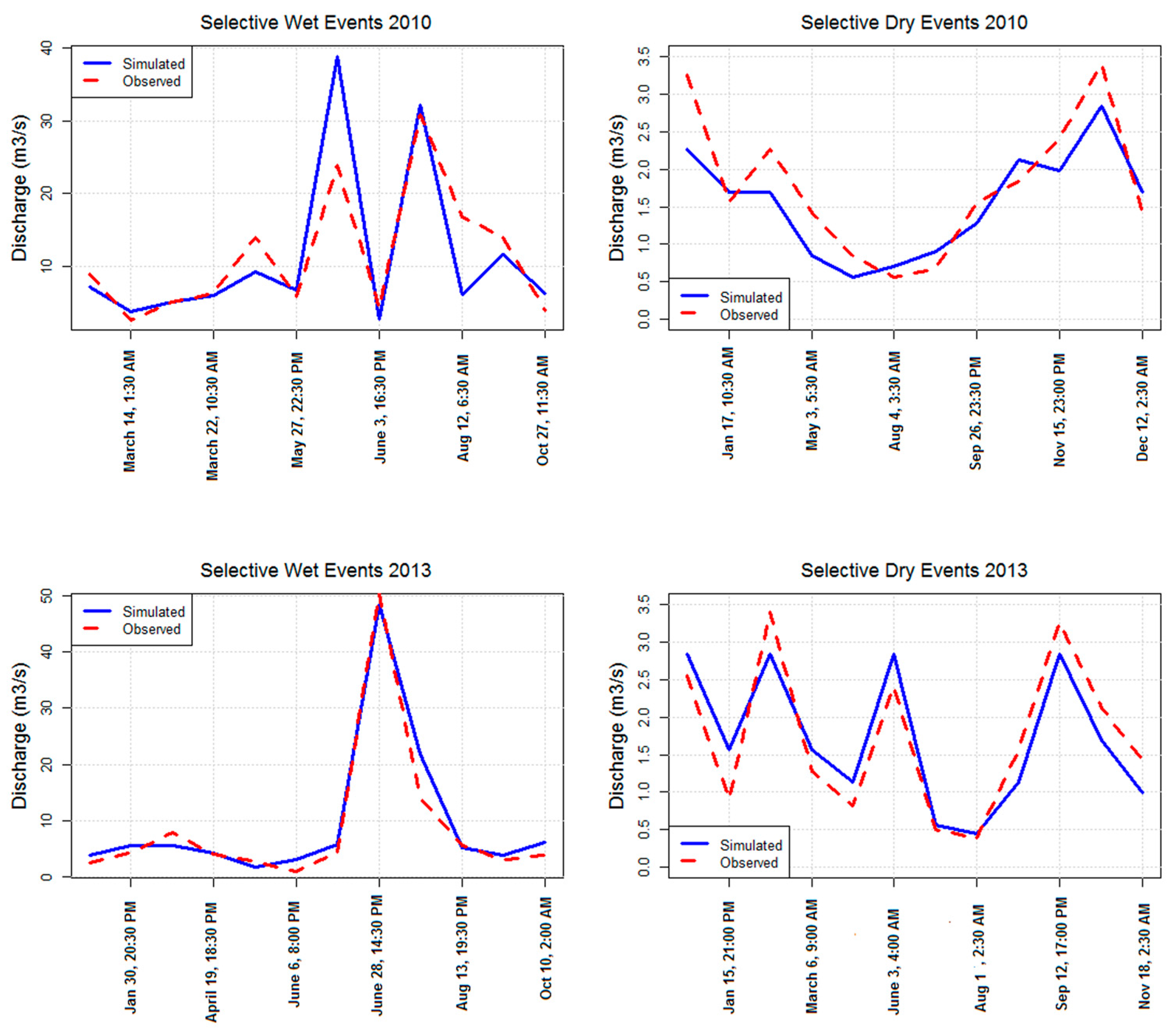
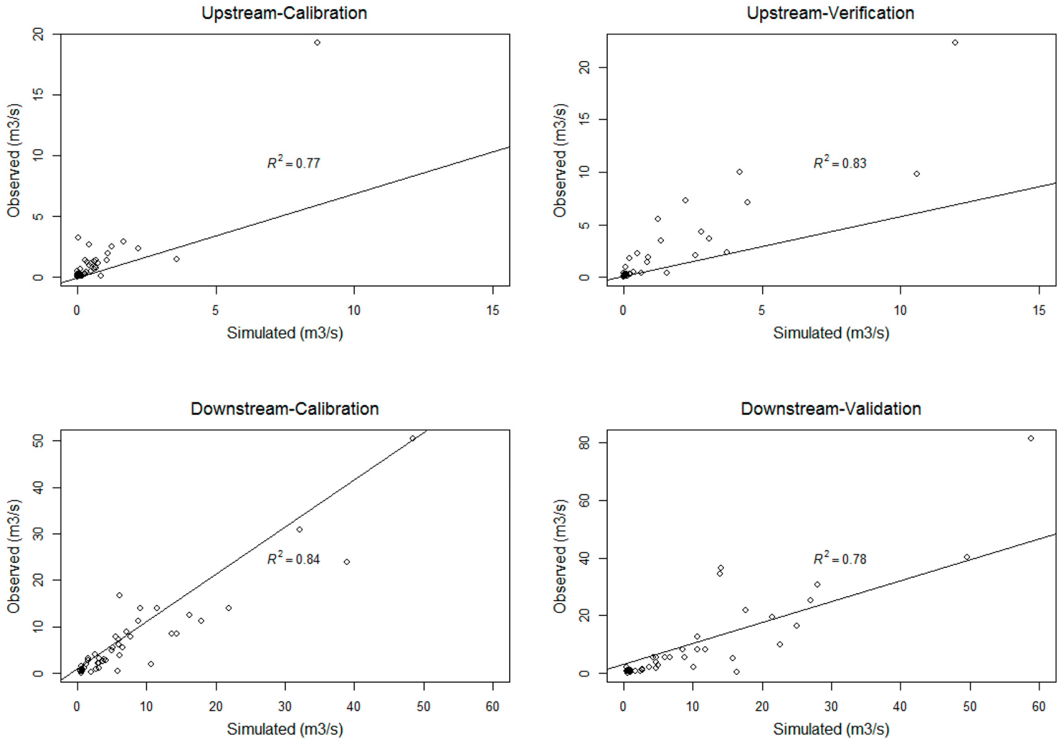
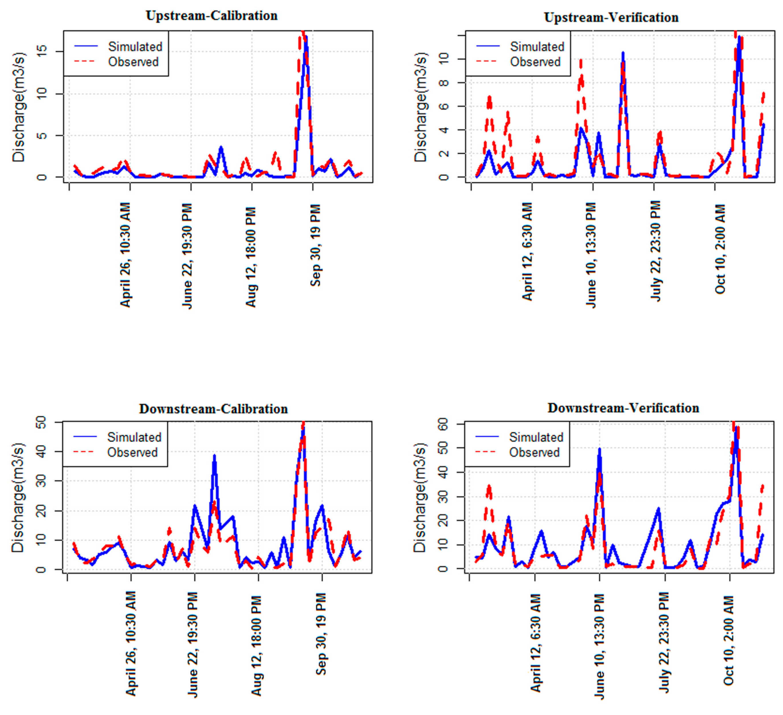
A hydrologic/hydraulic/water quality model (SWMM) was used to simulate a continuous rainfall-runoff response in an urban watershed, Difficult Run, Fairfax, VA. The model was then calibrated to observed conditions for peak flows, runoff volume, and water quality using two gauging stations in the watershed. The calibrated model was verified by assessing its performance against historical data. After calibration and verification, the impact of CC on the runoff volume and water quality in the watershed was assessed using downscaled precipitation and temperature data. Recent simulations from the NARCCAP were adapted for this purpose, using dynamic downscaling. The hydrology of the Difficult Run watershed was then simulated using SWMM, with the assistance of RSWMM for calibration, event processing and exceedance curve plotting for historical and future conditions. The following conclusions can be drawn from the study:

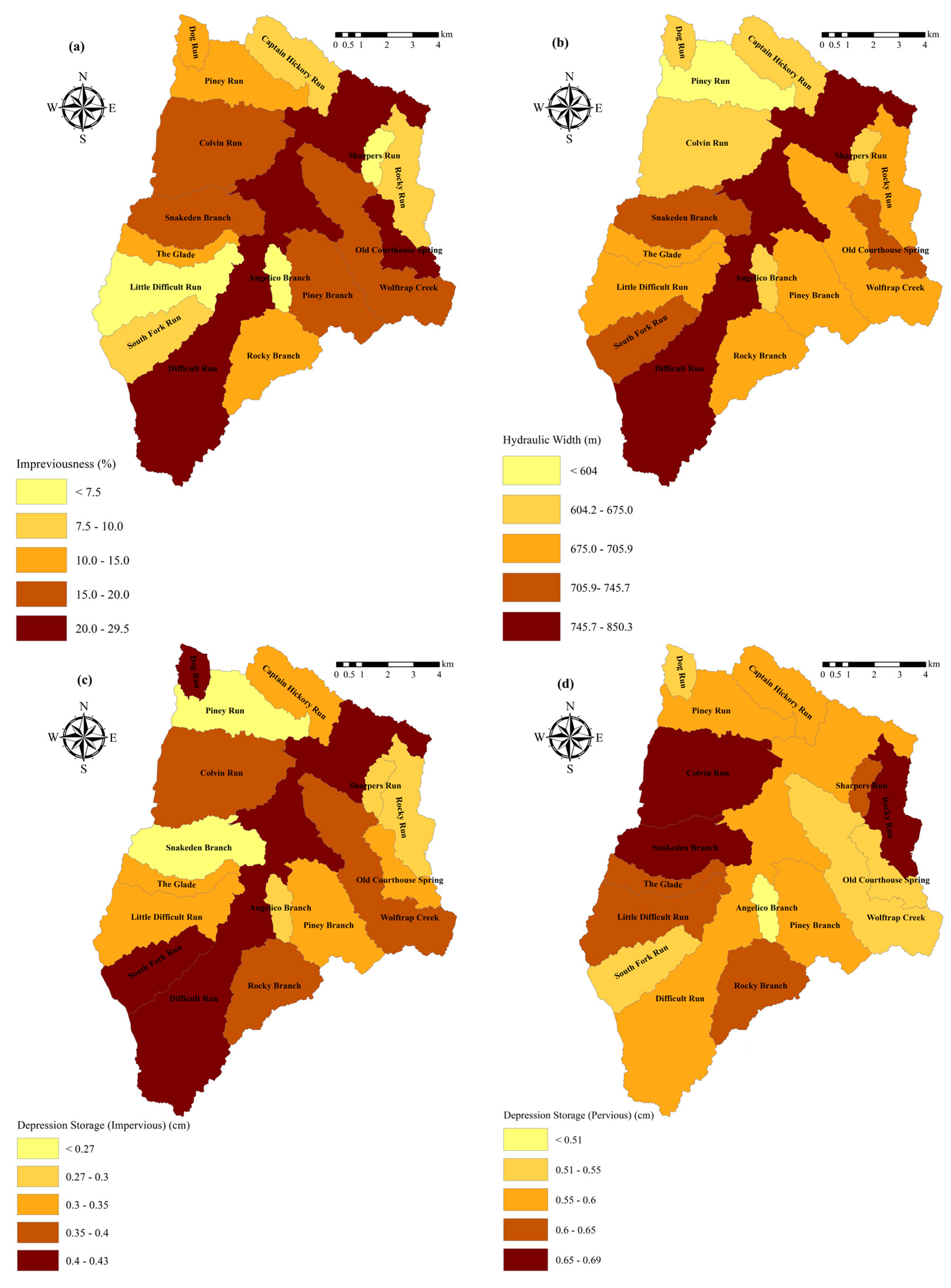
• Three SWMM parameters, including hydraulic width, imperviousness, and depression storage, were altered during calibration. Hydraulic width and imperviousness were the most sensitive parameters affecting peak flows.
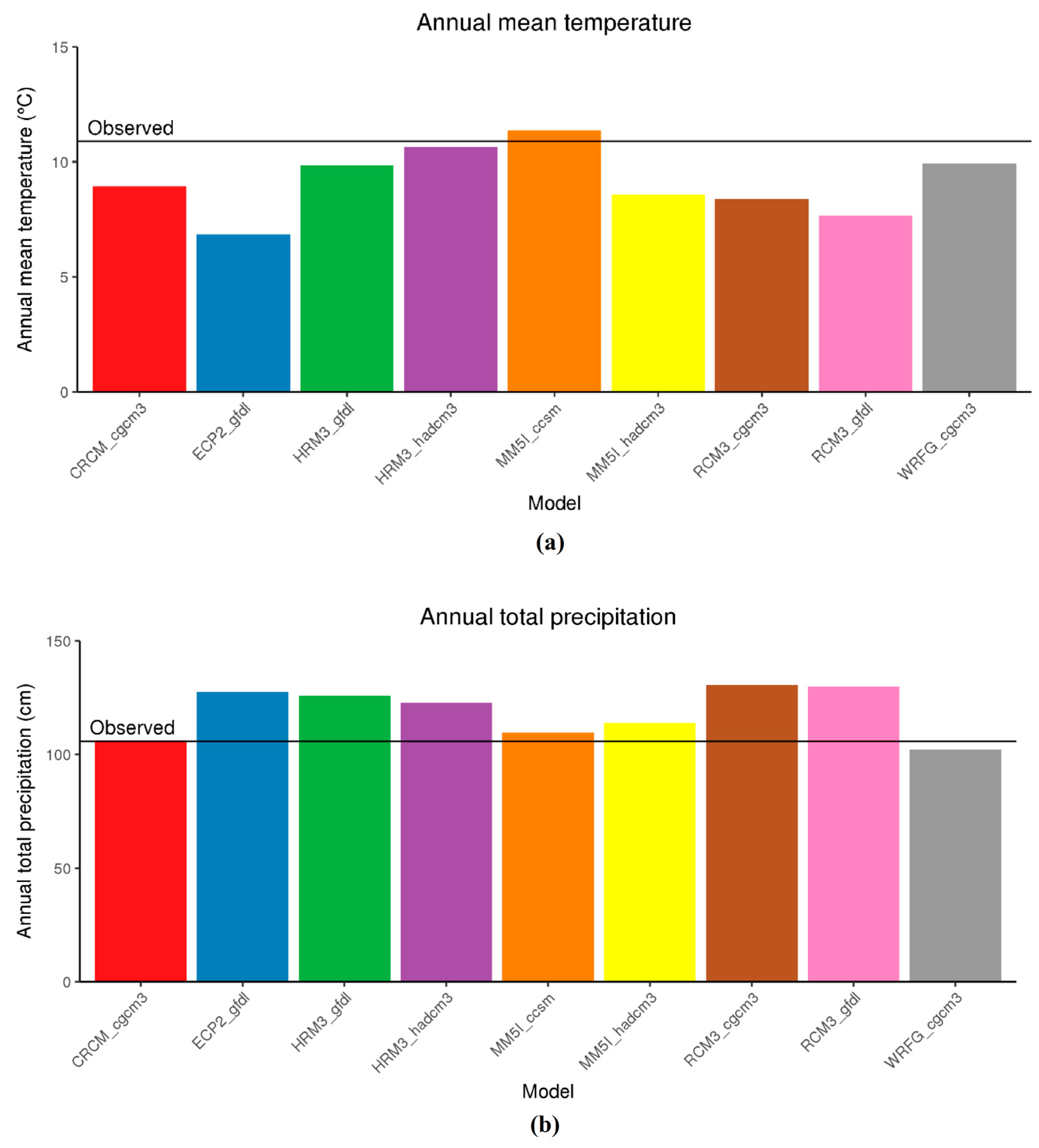
• NARCCAP and other dynamically downscaled model datasets are particularly useful for hydrological modeling because they provide downscaled data for all of the necessary variables from multiple global and regional models and are openly available online. Dynamical downscaling of the CMIP5 models is being performed by the North American Coordinated Regional Climate Downscaling Experiment (NA-CORDEX), but this project is not yet complete. Temperature and precipitation data from NA-CORDEX have been recently published, but other data that are needed for hydrological simulations, such as wind speed and radiation, are not yet available. Thus, the NARCCAP dataset is still the most current set of complete downscaled model data for our study area.
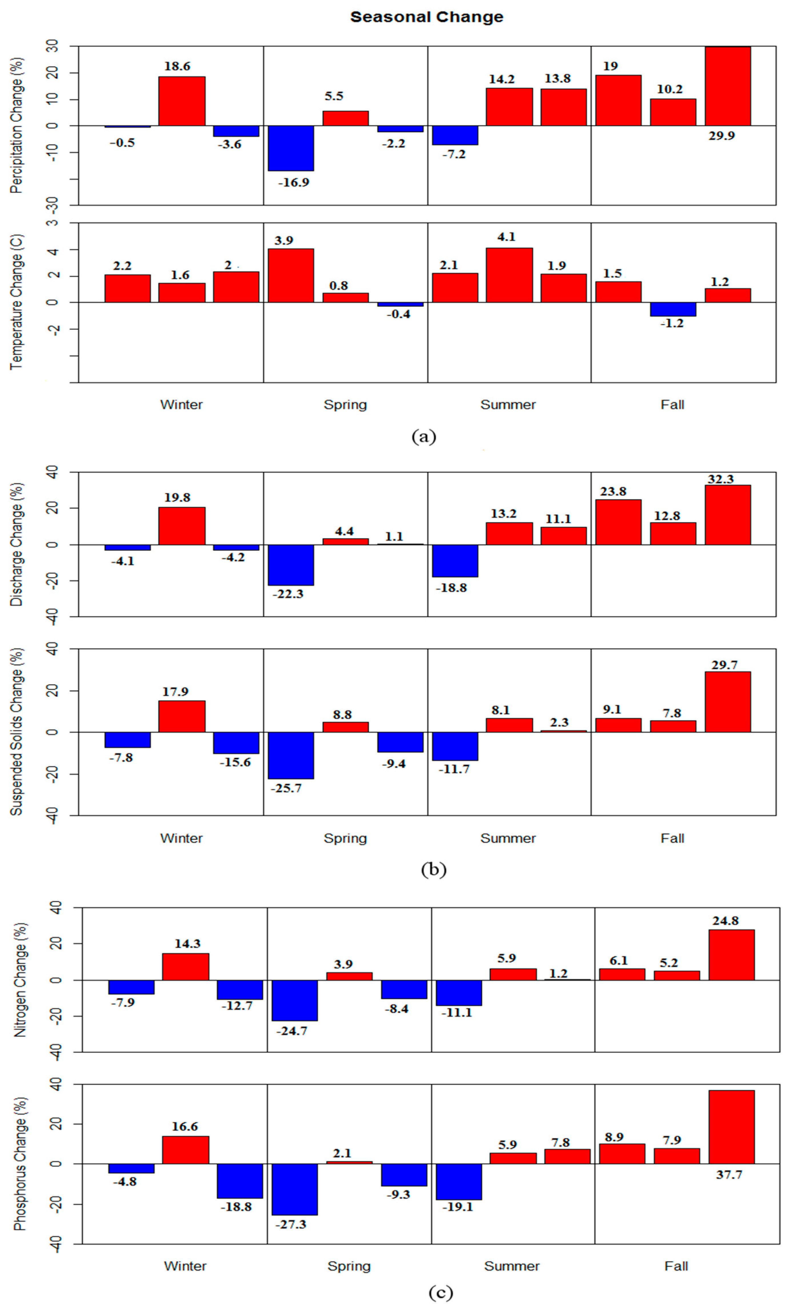
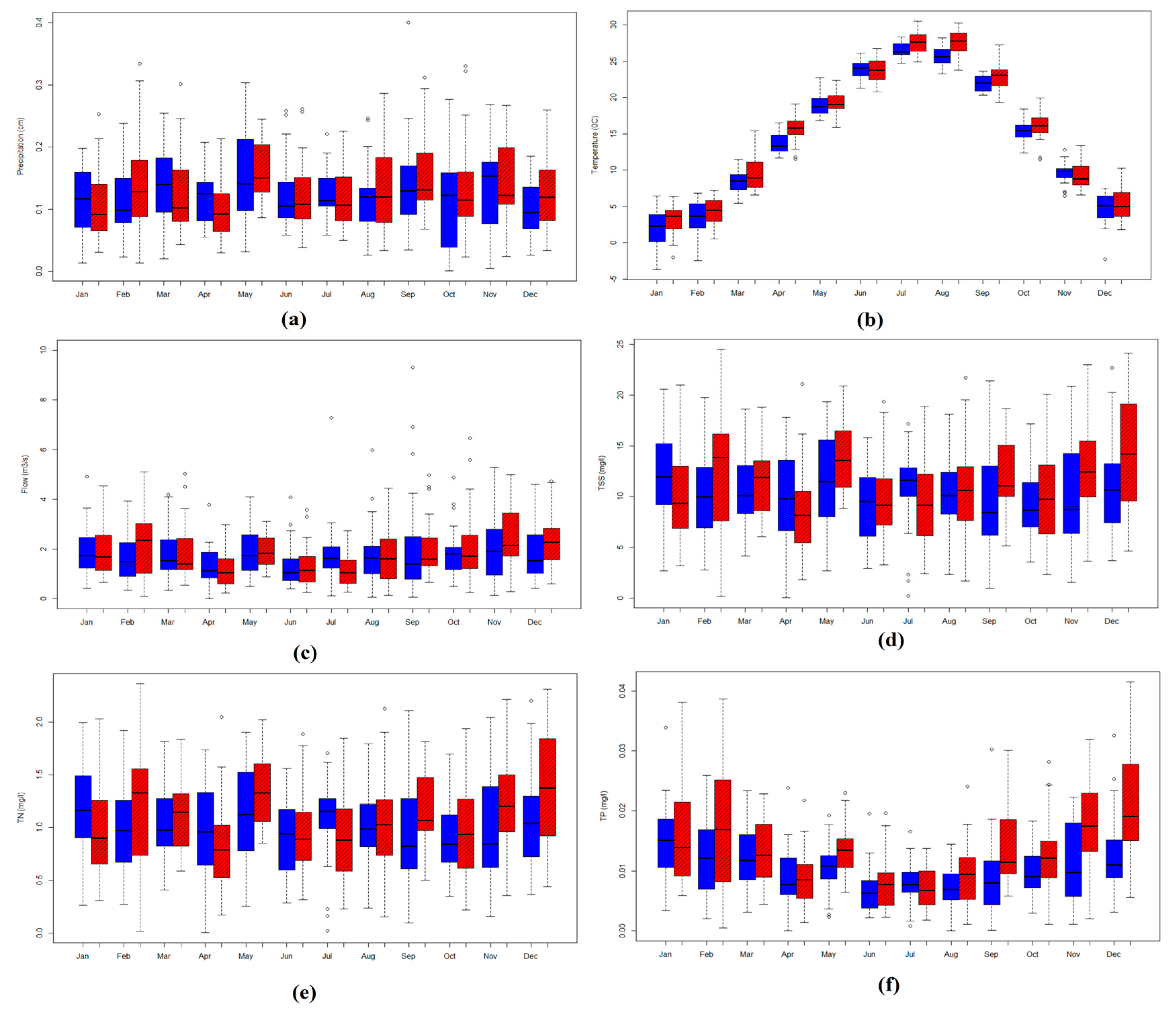
• The hydrological impact of the CC projection indicates that the mean annual runoff is predicted to increase by 6.5%, and TSS, TN, and TP are predicted to increase by 7.66%, 6.99%, and 8.1%, respectively. Statistically, only projected TP loads were significantly different than historical TP loads.
• The simulation results demonstrate that the mean, median, maximum, and the range between the 10th and 95th percentiles were projected to increase in the future with CC conditions. The interannual variability in the future is also projected to increase.
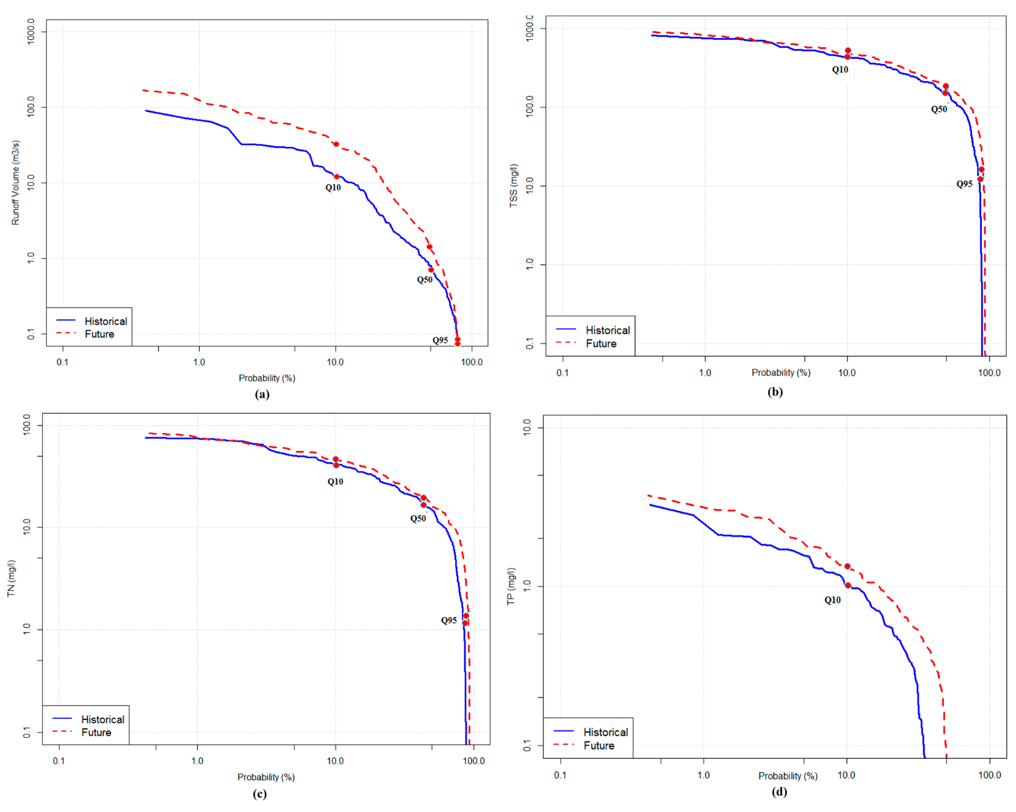
  Q10, Q50, and Q95 were compared using exceedance probability curves. Results show that these flow statistics are projected to increase in the future with CC; the greatest difference occurred at the 10th percentile for runoff volume.

The limitations of this analysis stem from the sources of uncertainty, which include: uncertainty in GCMs, including their inherent assumptions regarding future emission of greenhouse gases, uncertainty in the representation of climatology at regional and local scales, and uncertainty of parameters required for input in development of hydrological models. Analysis of uncertainty propagating through the multiple models and processes covered in this study was beyond the scope of this case study, but is a research recommendation. A key limitation of the case study analysis is the use of a single greenhouse emission scenario. However, the contribution of this paper is its development of methods for water quality modeling of an urban watershed subjected to CC. Methods used in this paper can be extended to incorporate a wide range of CC models.

Understanding CC effects on water quantity and quality in urban watersheds will help water resource managers and planners make better decisions in managing water resources issues. Studies such as these can assist them as they evaluate the complex physical, social and economic impacts of CC on urban communities. In addition, making predictions of the impact of CC will help improve the management of stormwater systems to reduce flooding and to produce better water quality through appropriate selection of SCMs.

References

1. Mishra, V.; Lettenmaier, D.P. Climatic trends in major U.S. urban areas, 1950–2009. Geophys. Res. Lett. 2011, 38, L16401. [Google Scholar] [CrossRef]
2. Hayhoe, K.; Wake, C.; Anderson, B.; Liang, X.-Z.; Maurer, E.; Zhu, J.; Bradbury, J.; DeGaetano, A.; Stoner, A.; Wuebbles, D. Regional climate change projections for the Northeast USA. Mitig. Adapt. Strateg. Glob. Chang. 2008, 13, 425–436. [Google Scholar] [CrossRef]
3. Najjar, R.G.; Pyke, C.R.; Adams, M.B.; Breitburg, D.; Hershner, C.; Kemp, M.; Howarth, R.; Mulholland, M.R.; Paolisso, M.; Secor, D.; et al. Potential climate-change impacts on the Chesapeake Bay. Estuar. Coast. Shelf Sci. 2010, 86, 1–20. [Google Scholar] [CrossRef]
4. Zahmatkesh, Z.; Burian, S.; Karamouz, M.; Tavakol-Davani, H.; Goharian, E. Low-impact development practices to mitigate climate change effects on urban stormwater runoff: Case study of new york city. J. Irrig. Drain. Eng. 2014, 141, 04014043. [Google Scholar] [CrossRef]
5. Semadeni-Davies, A.; Hernebring, C.; Svensson, G.; Gustafsson, L.-G. The impacts of climate change and urbanisation on drainage in Helsingborg, Sweden: Combined sewer system. J. Hydrol. 2008, 350, 100–113. [Google Scholar] [CrossRef]
6. Pavlovic, S.; Perica, S.; Martin, D.; Roy, I.; StLaurent, M.; Trypaluk, C.; Unruh, D.; Yekta, M.; Bonnin, G. NOAA Atlas 14: Updated Precipitation Frequency Estimates for the United States; National Weather Service: Silver Spring, MD, USA, 2013.
7. Ahmadisharaf, E.; Kalyanapu, A.J. Investigation of the impact of streamflow temporal variation on dam overtopping risk: Case study of a high-hazard dam. In Proceedings of the World Environmental and Water Resources Congress, Austin, TX, USA, 17–21 May 2015; pp. 1050–1057. [Google Scholar]
8. Madsen, T.; Figdor, E. When it Rains, it Pours: Global Warming and the Rising Frequency of Extreme Precipitation in the United States; Environment Texas Research & Policy Center: Austin, TX, USA, 2007; p. 47. [Google Scholar]
9. Moglen, G.; Rios Vidal, G. Climate Change and Storm Water Infrastructure in the Mid-Atlantic Region: Design Mismatch Coming? J. Hydrol. Eng. 2014, 11, 04014026. [Google Scholar] [CrossRef]
10. Peck, A.; Prodanovic, P.; Simonovic, S.P. Rainfall intensity duration frequency curves under climate change: City of London, Ontario, Canada. Can. Water Resour. J. 2012, 37, 177–189. [Google Scholar] [CrossRef]
11. Wright, L.; Chinowsky, P.; Strzepek, K.; Jones, R.; Streeter, R.; Smith, J.; Mayotte, J.-M.; Powell, A.; Jantarasami, L.; Perkins, W. Estimated effects of climate change on flood vulnerability of U.S. bridges. Mitig. Adapt. Strateg. Glob. Chang. 2012, 17, 939–955. [Google Scholar] [CrossRef]
12. Schoof, J.T. Scale Issues in the development of future precipitation scenarios. J. Contemp. Water Res. Educ. 2012, 147, 8–16. [Google Scholar] [CrossRef]
13. Fowler, H.J.; Wilby, R.L. Beyond the downscaling comparison study. Int. J. Climatol. 2007, 27, 1543–1545. [Google Scholar] [CrossRef]
14. Chen, J.; Brissette, F.P.; Chaumont, D.; Braun, M. Finding appropriate bias correction methods in downscaling precipitation for hydrologic impact studies over North America. Water Resour. Res. 2013, 49, 4187–4205. [Google Scholar] [CrossRef]
15. Wood, A.W.; Leung, L.R.; Sridhar, V.; Lettenmaier, D.P. Hydrologic implications of dynamical and statistical approaches to downscaling climate model outputs. Clim. Chang. 2004, 62, 189–216. [Google Scholar] [CrossRef]
16. Teutschbein, C.; Seibert, J. Bias correction of regional climate model simulations for hydrological climate-change impact studies: Review and evaluation of different methods. J. Hydrol. 2012, 456, 12–29. [Google Scholar] [CrossRef]
17. Gudmundsson, L.; Bremnes, J.; Haugen, J.; Engen-Skaugen, T. Technical Note: Downscaling RCM precipitation to the station scale using statistical transformations—A comparison of methods. Hydrol. Earth Syst. Sci. 2012, 16, 3383–3390. [Google Scholar] [CrossRef]
18. Lafon, T.; Dadson, S.; Buys, G.; Prudhomme, C. Bias correction of daily precipitation simulated by a regional climate model: A comparison of methods. Int. J. Climatol. 2013, 33, 1367–1381. [Google Scholar] [CrossRef]
19. Rosenberg, E.A.; Keys, P.W.; Booth, D.B.; Hartley, D.; Burkey, J.; Steinemann, A.C.; Lettenmaier, D.P. Precipitation extremes and the impacts of climate change on stormwater infrastructure in Washington State. Clim. Chang. 2010, 102, 319–349. [Google Scholar] [CrossRef]
20. Wang, L.; Chen, W. Equiratio cumulative distribution function matching as an improvement to the equidistant approach in bias correction of precipitation. Atmos. Sci. Lett. 2014, 15, 1–6. [Google Scholar] [CrossRef]
21. Natural Resources Conservation Service. WinTR-55 Watershed Hydrology; USDA Natural Resource Conservation Service: Washington, DC, USA, 2016.
22. U.S. Army Corps of Engineers. Hydrologic Modeling System HEC-HMS, Version 4.1; Hydrologic Engineering Center: Davis, CA, USA, 2016. [Google Scholar]
23. Danish Hydrauic Institute. Mike Urban; Danish Hydrauic Institute: Hørsholm, Denmark, 2016. [Google Scholar]
24. Rossman, L.A. Storm Water Management Model User’s Manual, Version 5.0; U.S. Environmental Protection Agency: Cincinatti, OH, USA, 2004.
25. Huber, W.C.; Dickinson, R.E.; Rosener, L.A.; Aldrich, J.A. Stormwater Management Model User’s Manual, Version 4; U.S. Environmental Protection Agency: Athens, GA, USA, 1988.
26. Zoppou, C. Review of urban storm water models. Environ. Modell. Softw. 2001, 16, 195–231. [Google Scholar] [CrossRef]
27. Elliott, A.; Trowsdale, S. A review of models for low impact urban stormwater drainage. Environ. Model. Softw. 2007, 22, 394–405. [Google Scholar] [CrossRef]
28. Warwick, J.; Tadepalli, P. Efficacy of SWMM Application. J. Water Res. Plan. Manag. 1991, 117, 352–366. [Google Scholar] [CrossRef]
29. Selvalingam, S.; Liong, S.Y.; Manoharan, P.C. Use of RORB and SWMM models to an urban catchment in Singapore. Adv. Water Res 1987, 10, 78–86. [Google Scholar] [CrossRef]
30. Campbell, C.W.; Sullivan, S.M. Simulating time-varying cave flow and water levels using the Storm Water Management Model. Eng. Geol. 2002, 65, 133–139. [Google Scholar] [CrossRef]
31. James, W.; Rossman, L.A.; James, W.R.C. User’s Guide to SWMM 5; Computational Hydraulics International: Guelph, ON, Canada, 2010; p. 905. [Google Scholar]
32. Zahmatkesh, Z.; Karamouz, M.; Goharian, E.; Burian, S. Analysis of the effects of climate change on urban storm water runoff using statistically downscaled precipitation data and a change factor approach. J. Hydrol. Eng. 2014, 20, 05014022. [Google Scholar] [CrossRef]
33. Bhaduri, B.; Minner, M. Long-term hydrologic impact of urbanization: A tale of two models. J. Water Resour. Plan. Manag. 2001, 127, 13–19. [Google Scholar] [CrossRef]
34. Barco, J.; Wong, K.M.; Stenstrom, M.K. Automatic Calibration of the U.S. EPA SWMM model for a large urban catchment. J. Hydraul. Eng. 2008, 134, 466–474. [Google Scholar] [CrossRef]
35. Kaushal, S.S.; Belt, K.T. The urban watershed continuum: Evolving spatial and temporal dimensions. Urban Ecosyst. 2012, 15, 409–435. [Google Scholar] [CrossRef]
36. Nelson, E.J.; Booth, D.B. Sediment sources in an urbanizing, mixed land-use watershed. J. Hydrol. 2002, 264, 51–68. [Google Scholar] [CrossRef]
37. Hatt, B.E.; Fletcher, T.D.; Walsh, C.J.; Taylor, S.L. The Influence of urban density and drainage infrastructure on the concentrations and loads of pollutants in small streams. Environ. Manag. 2004, 34, 112–124. [Google Scholar] [CrossRef] [PubMed]
38. National Research Council. Clean Coastal Waters: Understanding and Reducing the Effects of Nutrient Pollution; National Academies Press: Washington, DC, USA, 2000. [Google Scholar]
39. U.S. EPA. Chesapeake Bay Total Maximum Daily Load for Nitrogen, Phosphorous, and Sediment in: USEPA Region III; United States Environmental Protection Agency: Philadelphia, PA, USA, 2010; p. 261.
40. Lee, Y.J.; Boynton, W.R.; Li, M.; Li, Y. Role of late winter–spring wind influencing summer hypoxia in Chesapeake Bay. Estuar. Coasts 2013, 36, 683–696. [Google Scholar] [CrossRef]
41. Scully, M.E. The importance of climate variability to wind-driven modulation of hypoxia in Chesapeake Bay. J. Phys. Oceanogr. 2010, 40, 1435–1440. [Google Scholar] [CrossRef]
42. Hathaway, J.M.; Brown, R.A.; Fu, J.S.; Hunt, W.F. Bioretention function under climate change scenarios in North Carolina, USA. J. Hydrol. 2014, 519, 503–511. [Google Scholar] [CrossRef]
43. Schaefer, S.C.; Alber, M. Temperature controls a latitudinal gradient in the proportion of watershed nitrogen exported to coastal ecosystems. Biogeochemistry 2007, 85, 333–346. [Google Scholar] [CrossRef]
44. Fairfax County. Difficult Run Watershed Management Plan; Government Center Parkway: Fairfax, VA, USA, 2007.
45. Liu, J.; Sample, D.; Bell, C.; Guan, Y. Review and research needs of bioretention used for the treatment of urban stormwater. Water 2014, 6, 1069–1099. [Google Scholar] [CrossRef]
46. Jastram, J.D. Streamflow, Water Quality, and Aquatic Macroinvertebrates of Selected Streams in Fairfax County, Virginia, 2007–2012; Scientific Investigations Report 2014-5073; U.S. Geological Survey Will: Reston, VA, USA, 2014; p. 82.
47. Ahmadisharaf, E.; Tajrishy, M.; Alamdari, N. Integrating flood hazard into site selection of detention basins using spatial multi-criteria decision-making. J. Environ. Plan. Manag. 2016, 59, 1397–1417. [Google Scholar] [CrossRef]
48. Drake, A.A. Geologic Map of the Fairfax Quadrangle; U.S. Geological Survey: Fairfax County, VA, USA, 1986.
49. Dicken, C.; Nicholson, S.; Horton, J.; Kinney, S.; Gunther, G.; Foose, M.; Mueller, J. Preliminary Integrated Geologic Map Databases for the United States; U.S. Geologic Survey: Fairfax County, VA, USA, 2007.
50. Natural Resources Conservation Service. Web Soil Survey. Available online: http://websoilsurvey.nrcs.usda.gov/ (accessed on 17 May 2015).
51. Rossman, L.A. Storm Water Management Model Reference Manual: Volume I, Hydrology; US Environmental Protection Agency: Cincinnati, OH, USA, 2015.
52. Mearns, L.O.; Gutowski, W.; Jones, R.; Leung, R.; McGinnis, S.; Qian, Y. A regional climate change assessment program for North America. Earth Space Sci. News 2009, 90, 311. [Google Scholar] [CrossRef]
53. Hirschman, D.; Collins, K.; Schueler, T. Technical Memorandum: The Runoff Reduction Method; Center for Watershed Protection & Chesapeake Stormwater Network: Ellicott City, MD, USA, 2008. [Google Scholar]
54. U.S. EPA. Stormwater Best Management Practices (BMP) Performance Analysis; Tetra Tech, Inc.: Fairfax, VA, USA, 2010; p. 232. [Google Scholar]
55. Park, D.; Roesner, L.A. Evaluation of pollutant loads from stormwater BMPs to receiving water using load frequency curves with uncertainty analysis. Water Res. 2012, 46, 6881–6890. [Google Scholar] [CrossRef] [PubMed]
56. Chretien, F.; Gagnon, P.; Theriault, G.; Guillou, M. Performance analysis of a wet-retention pond in a small agricultural catchment. J. Environ. Eng. 2016, 142, 10. [Google Scholar] [CrossRef]
57. R Team. R: A Language and Environment for Statistical Computing; R Foundation for Statistical Computing: Vienna, Austria, 2014. [Google Scholar]
58. Fuka, D.R.; Walter, M.T.; MacAlister, C.; Steenhuis, T.S.; Easton, Z.M. SWATmodel: A multi-operating system, multi-platform SWAT model package in R. J. Am. Water Res. Assoc. 2014, 50, 1349–1353. [Google Scholar] [CrossRef]
59. Alamdari, N. Development of a robust automated tool for calibrating a SWMM watershed model. In Proceedings of the World Environmental and Water Resources Congress, West Palm Beach, FL, USA, 22–26 May 2016; p. 221. [Google Scholar]
60. Temprano, J.; Arango, O.; Cagiao, J.; Suarez, J.; Tejero, I. Stormwater quality calibration by SWMM: A case study in northern Spain. Water SA 2006, 32, 55–63. [Google Scholar] [CrossRef]
61. CDM Smith Inc. NETSTORM Version 2015.2. Available online: http://www.dynsystem.com/netstorm/ (accessed on 20 March 2015).
62. Santhi, C.; Arnold, J.G.; Williams, J.R.; Dugas, W.A.; Srinivasan, R.; Hauck, L.M. Validation of the SWAT model on a large river basin with point and nonpoint sources. J. Am. Water Res. Assoc. 2001, 37, 1169–1188. [Google Scholar] [CrossRef]
63. Van Liew, M.W.; Arnold, J.G.; Garbrecht, J.D. Hydrologic simulation on agricultural watersheds: Choosing between two models. Trans. ASAE 2003, 46, 1539–1551. [Google Scholar] [CrossRef]
64. Nash, J.E.; Sutcliffe, J.V. River flow forecasting through conceptual models part I—A discussion of principles. J. Hydrol. 1970, 10, 282–290. [Google Scholar] [CrossRef]
65. Gupta, H.V.; Sorooshian, S.; Yapo, P.O. Status of automatic calibration for hydrologic models: Comparison with multilevel expert calibration. J. Hydrol. Eng. 1999, 4, 135–143. [Google Scholar] [CrossRef]
66. Nakićenović, N.; Swart, R. (Eds.) Special report on emission scenarios. In Emssions Scenarios; Cambridge Univesity Press: Cambridge, UK, 2000; p. 570. [Google Scholar]
67. Xia, Y.L.; Mitchell, K.; Ek, M.; Sheffield, J.; Cosgrove, B.; Wood, E.; Luo, L.F.; Alonge, C.; Wei, H.L.; Meng, J.; et al. Continental-scale water and energy flux analysis and validation for the North American Land Data Assimilation System project phase 2 (NLDAS-2): 1. Intercomparison and application of model products. J. Geophys. Res. Atmos. 2012, 117. [Google Scholar] [CrossRef]
68. Gao, H.; Tang, Q.; Shi, X.; Zhu, C.; Bohn, T.; Su, F.; Sheffield, J.; Pan, M.; Lettenmaier, D.; Wood, E.F. Water budget record from Variable Infiltration Capacity (VIC) model. In Algorithm Theoretical Basis Document for Terrestrial Water Cycle Data Records; University of Washington: Washington, DC, USA, 2010. [Google Scholar]
69. Shapiro, S.S.; Wilk, M.B. An analysis of variance test for normality (complete samples). Biometrika 1965, 52, 591–611. [Google Scholar] [CrossRef]
70. Moriasi, D.N.; Arnold, J.G.; Van Liew, M.W.; Bingner, R.L.; Harmel, R.D.; Veith, T.L. Model evaluation guidelines for systematic quantification of accuracy in watershed simulations. Trans. ASAE 2007, 50, 885–900. [Google Scholar] [CrossRef]
Figure 1. Subwatershed location map.
Water 09 00464 g001
Figure 2. (a) Annual mean temperature for nine global climate models/regional climate models (GCM-RCM); (b) Annual mean precipitation for nine GCM-RCM.
Water 09 00464 g002
Figure 3. Calibration and validation results at the Difficult Run upstream and downstream gauging stations.
Water 09 00464 g003
Figure 4. Comparison of observed and simulated data at the Difficult Run upstream and downstream gauging stations for calibration (2010) and verification (2013) periods.
Water 09 00464 g004
Figure 5. Comparison of observed and simulated data at the Difficult Run downstream gaging station for selective events.
Water 09 00464 g005
Figure 6. Model calibrated parameters for sub-catchments in Difficult Run watershed, (a) imperviousness (percentage); (b) hydraulic width (m); (c) depression storage (of impervious portion) (cm); and (d) depression storage (of pervious portion) (cm).
Water 09 00464 g006
Figure 7. (a) Water quality calibration results at the Difficult Run upstream gauging station; (b) Water quality calibration results at the Difficult Run downstream gauging station.
Water 09 00464 g007
Figure 8. Seasonal changes. (a) Precipitation (top) and temperature (bottom); (b) flow (top) and Total Suspended Solids (TSS) (bottom); (c) Total Nitrogen (TN) (top) and Total Phosphorus (TP) (bottom).
Water 09 00464 g008
Figure 9. Interannual variability of: (a) precipitation; (b) temperature; (c) flow; (d) TSS; (e) TN; and (f) TP. Historical is shown in blue and projected in red cross hatching.
Water 09 00464 g009
Figure 10. Exceedance probability curves for (a) runoff volume; (b) TSS; (c) TN; and (d) TP.
Water 09 00464 g010