Impact of Future Climate Change on Regional Crop Water Requirement—A Case Study of Hetao Irrigation District, China

1
Institute of Soil and Water Conservation, Northwest A&F University, Yangling 712100, China
2
Institute of Water Saving Agriculture in Arid regions of China, Northwest A&F University, Yangling 712100, China
3
Key Laboratory of Agricultural Soil and Water Engineering in Arid and Semiarid Areas, Ministry of Education, Northwest A&F University, Yangling 712100, China
4
College of Water Resources and Architectural Engineering, Northwest A&F University, Yangling 712100, China
5
Institute of Soil and Water Conservation, Chinese Academy of Sciences and Ministry of Water Resources, Yangling 712100, China
*
Authors to whom correspondence should be addressed.
Water 2017, 9(6), 429; https://doi.org/10.3390/w9060429
Submission received: 11 April 2017
/
Revised: 6 June 2017
/
Accepted: 8 June 2017
/
Published: 13 June 2017
(This article belongs to the Special Issue Adaptation Strategies to Climate Change Impacts on Water Resources)
Abstract
:Water shortage is a limiting factor for agricultural production in China, and climate change will affect agricultural water use. Studying the effects of climate change on crop irrigation requirement (CIR) would help to tackle climate change, from both food security and sustainable water resource use perspectives. This paper applied SDSM (Statistical DownScaling Model) to simulate future meteorological parameters in the Hetao irrigation district (HID) in the time periods 2041–2070 and 2071–2099, and used the Penman–Monteith equation to calculate reference crop evapotranspiration (ET0), which was further used to calculate crop evapotranspiration (ETc) and crop water requirement (CWR). CWR and predicted future precipitation were used to calculate CIR. The results show that the climate in the HID will become warmer and wetter; ET0 would would increase by 4% to 7%; ETc and CWR have the same trend as ET0, but different crops have different increase rates. CIR would increase because of the coefficient of the increase of CWR and the decrease of effective precipitation. Based on the current growing area, the CIR would increase by 198 × 106 to 242 × 106 m3 by the year 2041–2070, and by 342 × 106 to 456 × 106 m3 by the years 2071–2099 respectively. Future climate change will bring greater challenges to regional agricultural water use.
1. Introduction
According to the Assessment Report 5 of the Intergovernmental Panel on Climate Change (IPCC), the global surface temperature has increased by 0.65–1.06 °C during the years 1880–2012, and the rate of the temperature increase after 1951 has been approximately 0.12 °C per 10 years, which is almost twice the rate since 1880. Furthermore, it is predicted that by the end of the 21st century (2081–2100), the average global surface temperature will be 1.5–2.0 °C higher than that in the years 1850–1900 [1,2]. Climate change could not only affect global food production and supply [3], but can also impact the quality and safety of agricultural products [4,5]. Therefore, the world’s Food and Agriculture Organization (FAO) has made it a worldwide challenge to cope with climate change when solving world’s food supply problem and relieving hunger [6]. Climate change would have impacts on crop growth and water consumption pattern, as well as the quantity of irrigation water that crops require to grow well [7,8,9]. Exploring the changes in crop water requirement (CWR) and crop irrigation requirement (CIR) under the climate change circumstance could provide a theoretical basis for the design of irrigation water conservation facilities and agricultural water resources management.
General circulation models (GCMs) can simulate the important characteristics of future climate on a large scale very well in the study of regional climate change; however, the GCMs have limited value because they have a low spatial resolution and lack the regional climate information. Currently, there are two ways to make up for the inadequacy of GCMs in predicting regional climate change: one is to develop new GCMs with higher resolution, and another is to downscale GCMs to the regional scale. Due to the large amount of calculation required to improve the spatial resolution of the GCMs, downscaling techniques have gained in popularity [10]. Downscaling techniques can be further divided into dynamical downscaling and statistical downscaling. Dynamical downscaling is actually to build a regional climate model which has a clear physical meaning and will not be affected by the observation data; however, it also has some disadvantages. For example, it requires significant computing resources and is not readily transferred to new regions or domains. Statistical downscaling is based on the view that the regional climate is conditioned by the large-scale climatic state and local physiographic features. From this perspective, regional climate information can be derived from a statistical model which relates large-scale climate variables to regional variables. Although this method cannot be interpreted physically, it is computationally inexpensive and can be used to provide site-specific information. Statistical downscaling techniques are also widely used because they include three major types of methods (i.e., weather classification, regression models, and weather generators [11,12]), providing more choice to its users.
The studies of the impact of climate change on reference crop evapotranspiration (ET0) have different results in different study areas. Reference [13] used the LARS-WG (Long Ashton Research Station-Weather Generator) to generate future climate data in Suwon, South Korea, and found that the ET0 during the years 2080–2099 would be nearly 100 mm larger than of 1973–2088. In reference [14], the future ET0 in Puerto Rico was calculated, and the results show that the ET0 would keep an upward trend in the following 100 years under A2 scenario. The generalized linear model (GLM) was used in reference [15] to estimate the future ET0 in the UK, and the results indicate that the southern part of the UK will be more sensitive to the change in ET0 than the north. Reference [16] downscaled ET0 during 2011–2099 from HadCM3 (Hadley Centre Coupled Model, version 3) outputs by SDSM (Statistical DownScaling Model) in the Loess Plateau of China, finding a continuous increase and a possible increasing gradient from northeast to southwest region in ET0 in the 21st century. These theses mainly focus on the variations of the temporal and spatial aspects of future ET0, but they pay less attention to how the change of ET0 would affect the agricultural water use.
The Hetao irrigation district (HID) is one of the largest irrigation districts in addition to being an important commodity grain production base in China. It is of great significance to study how the climate, the future ET0 and CWR of HID would change, because the study would guide agricultural production planning in this area. This paper adopts two emission scenarios released by the IPCC; i.e., A2 (under this scenario, the global population continues to increase, and the economy grows rapidly) and B2 (under this scenario, the growth of population is slower than under A2, and a sustainable development strategy is adopted), and then use the Statistical DownScaling Model (SDSM) to predict main meteorological parameters in the time periods 2041–2070 and 2071–2099 in the HID under scenarios A2 and B2. The change of each parameter in the future are analyzed, and the future ET0 and crop evapotranspiration (ETc) of HID—which can provide a reference for the agricultural production—are calculated and analyzed.
2. Material and Methods
2.1. Study Area
The HID (Figure 1) is in western Inner Mongolia, China (40°19′–41°18′ N, 106°20′–109°19′ E), and is the largest gravity irrigation district in Asia [17]. It is located in the continental monsoon climate zone, which means that it has low precipitation, high evaporation, strong wind, large differences in temperature, and long sunshine hours. The annual average temperature is 6–8 °C, and the weather is dry and hot in the summer and severely cold with little snow in winter. The annual precipitation is 130–215 mm, of which 70% is during summer and autumn. The annual evaporation is 2100–2300 mm, which is ten times as large as the precipitation. The irrigation area currently covers 574 × 103 ha, and the annual amount of irrigation water is about 5 × 10⁹ m3, mainly derived from the Yellow River. The major crops grown are spring wheat, maize, and sunflower [18,19].
2.2. Data
(1) Observed data: The China Meteorological Administration [20] offers daily meteorological data including maximum temperature (Tmax, °C), minimum temperature (Tmin, °C), relative humidity (RH, %), wind speed (WS, m·s−1), precipitation (P, mm), and sunshine hours (SH, h) during the period of 1980–2013 of eight meteorological stations in and around HID, and geological data including the altitude, longitude, and latitude of each meteorological station .
(2) Reanalysis data: The National Centre for Environmental Prediction (NCEP) [21,22] provides daily reanalysis data of 26 factors including mean temperature, mean sea level pressure, near surface relative humidity, near surface specific humidity, 500 hPa geopotential height, 850 hPa geopotential height, and relative humidity, geostrophic airflow velocity, vorticity, zonal velocity component, meridional velocity component, wind direction and divergence at surface, 500 hPa height, and 850 hPa height respectively. The grid resolution is 2.5 degrees of latitude by 2.5 degrees of longitude.
2.3. Calculation of ET0, ETc, and Effective Precipitation (PE)
The reference crop evapotranspiration (ET0) is calculated according to the FAO Penman–Monteith equation [25] as follows:
where is the slope of the vapor pressure curve (kPa·°C−1); is the net radiation at the crop surface (MJ·m−2·d−1); G is the soil heat flux density (MJ·m−2·d−1); γ is the psychrometric constant (kPa·°C−1); T is the average air temperature (°C); is the wind speed measured at 2 m height (m·s−1); is the saturation vapor pressure (kPa); and is the actual vapor pressure (kPa)
Evapotranspiration over the crop-growing period (ETc) is calculated as follows:
where KC is the crop coefficient (which is dimensionless), and in this paper we assume that the future KC will not change.
Effective precipitation (PE) over the growth period is calculated as follows [26]:
where P is the precipitation during crop growing period (mm).
Crop irrigation requirement (CIR) is the amount of water other than precipitation that crops need to meet water demand, and can be calculated as follows:
where CIR is the crop irrigation requirement, ETc the crop evapotranspiration and PE the effective precipitation over the crop growth period.
The total crop irrigation requirement in the study area can be calculated as follows:
where is the planting area of crop , the irrigation requirement of crop .
2.4. Statistical DownScaling Model
The Statistical DownScaling Model is a decision support tool [27] now at version 5.2. It combines regression models and weather generators, and is easy and convenient to use.
The SDSM model was built by inputting the daily observed data and the NCEP data (the data with time period of 1980–1999 are used to calibrate the model and 2000–2013 to validate model). This model was then applied to simulate the present climate by inputting HadCM3 data under A2 and B2 scenarios within the time period of 1980–2013. The control area in HID of each meteorological station—which is the base of the computation of the weight index—was calculated by the Thiessen polygon, and the climate of HID was the weight average of the meteorological parameters of related meteorological stations. Table 1 shows the results of the evaluation indicators under A2 and B2 scenarios, among which the Tmax, Tmin, SH, WS, and P were the result of downscaling, and ET0 was calculated by Equation (1).
To evaluate the results of the SDSM, this paper used R2 and Nash–Sutcliffe efficiency coefficient (E) as evaluation indicators.
where Q0 is the observed data, Qm is the simulated data, Qt is the value at the moment t, and is the average value of the observed data. The range of E is (−∞,1]; if E is close to 1, it means that the simulation result is reliable; if E is close to 0, it means that the simulation result is similar to the average value of the observed data; and if E is less than 0, it means that the result is undependable.
The R2 and E values of each parameter under the two scenarios are greater than 0.85, which means the model is reliable and can simulate the observed data in HID very well. It is fair to say that the SDSM could be applied to process the output of HadCM3 in HID.
3. Results
3.1. Temporal and Spatial Analysis of Meteorological Parameters
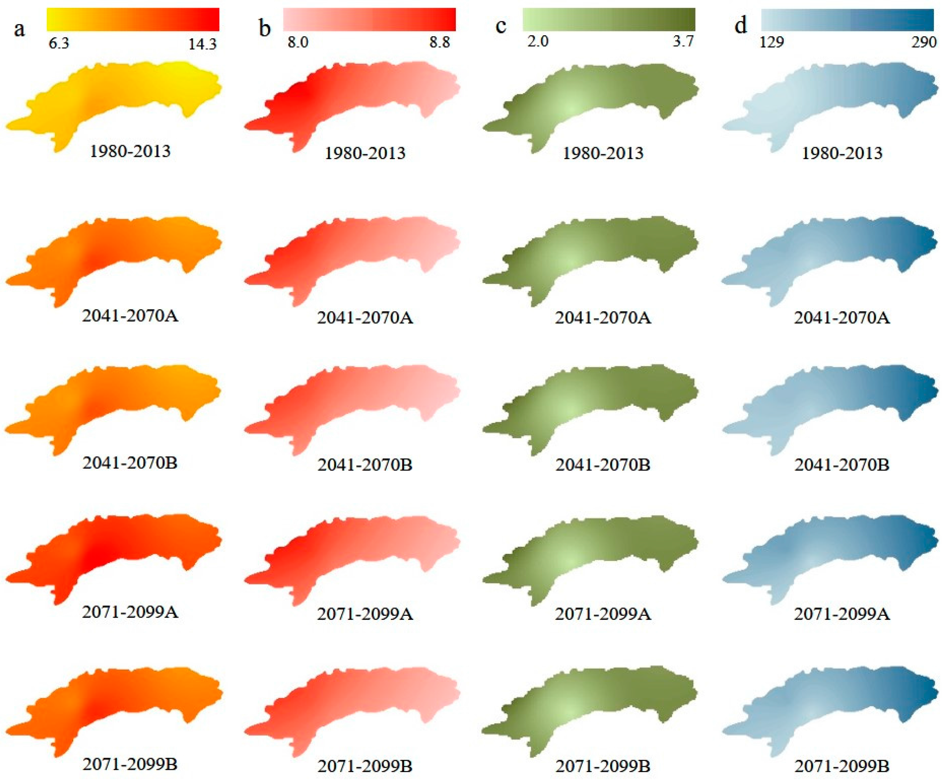
The average value of each parameter and their spatial distribution in different time periods are shown in Table 2 and Figure 2, respectively.
In the last decades of 21st century, the Tmin and Tmax of HID under scenario A2 would rise to 5.4 and 18.5 °C, respectively, and the average temperature is about 4 °C higher than the present stage. Temperature under scenario B2 increases relatively less with the increment 4.2 and 17.1 °C respectively—3 °C higher than the present stage. In terms of the SH, the phenomenon shows under both scenarios that during the years 2041-2070 the SH reaches its lowest value, while in the years 2071–2099 the value goes up but is still lower than that of the present stage. The SH under scenario A2 is longer than that under B2 scenario during the same time period, and the SH during the years 2041–2070 under scenario B2 is the lowest with only 8.5 h, which is 1.28% lower than that of the present stage. The precipitation in the years 2041–2070 and 2071–2099 does not have much difference under A2 or B2 scenario, but compared with the value of the present stage, P would increase by about 20 mm under scenario B2 and just a little bit less under A2. The wind speed and relative humidity in HID would not change significantly. Overall, the climate in HID would get warmer and wetter.
In terms of the spatial distribution, the maximum average annual temperature is 9.2 °C, which shows in the southern of the middle of HID during the present stage, and the minimum shows in western and northern of HID. The WS has a spatial distribution contrary to that of temperature, and its highest value is 3.5 m·s−1 and lowest 2 m·s−1 during the present stage. The SH peaks at 8.8 h during the present stage in the northwestern part of HID, while in the east the value shrinks down to just over 8 h; its spatial distribution shows a trend of decreasing from west to east, which is opposite to the distribution of precipitation whose lowest value is only 129 mm, shown in the west, and highest value is more than 240 mm, shown is the east. In the future, the spatial distribution of precipitation would change slightly with a decreasing trend in the middle area of HID, and it is more distinct under scenario A2. The spatial distribution pattern of other parameters does not change much, but the range of the values would change—especially the value of temperature, which will increase notably.
3.2. Temporal and Spatial Analysis of ET0
The change of meteorological parameters will cause a change in ET0. Figure 3 shows that during 1990–2003, the ET0 was below or just slightly above the average ET0 (1318 mm), while after 2003 the phenomenon reversed and in most years the ET0 was much higher than the average value. The climate inclination rate during the present stage is 11.5 mm per 10a, which means, on average, the ET0 rose 1.15 mm per year during this period of time. However, in the future (2021–2099), the average increment of ET0 is 2.28 mm per year under scenario A2, which is almost twice the present increasing rate; the rate under scenario B2 is 1.23 mm per year. ET0 would increase by 6.09% and 12.19% during the years 2041–2070 and 2071–2099, respectively, under scenario A2. The increase trend is the same under scenario B2, wherein the growth rate would increase over time, and the increments during the years 2041–2070 and 2071–2099 are 3.88% and 7.48%, respectively. Based on the fact that SH, WS, and RH would not change much in the future while the temperature would rise, it can be concluded that the increase of ET0 is mostly affected by the increase of temperature in HID. The temperature would maintain the growing trend in the future and would be higher under scenario A2 than under B2, and thus so would ET0. The spatial distribution of meteorological factors that affect ET0 would remain almost the same (Figure 2), so it is deducible that the spatial distribution of ET0 would hardly change (Figure 4). The highest value of ET0 shown in the west of HID and the lowest value in the east of HID.
Overall, with the change of meteorological parameters, ET0 in HID would continue to grow, which would cause a rise in CWR and further influence the hydrologic cycle, water balance, and agricultural production in the district.
3.3. Future Crop Water Requirement in Potential Climate Scenarios
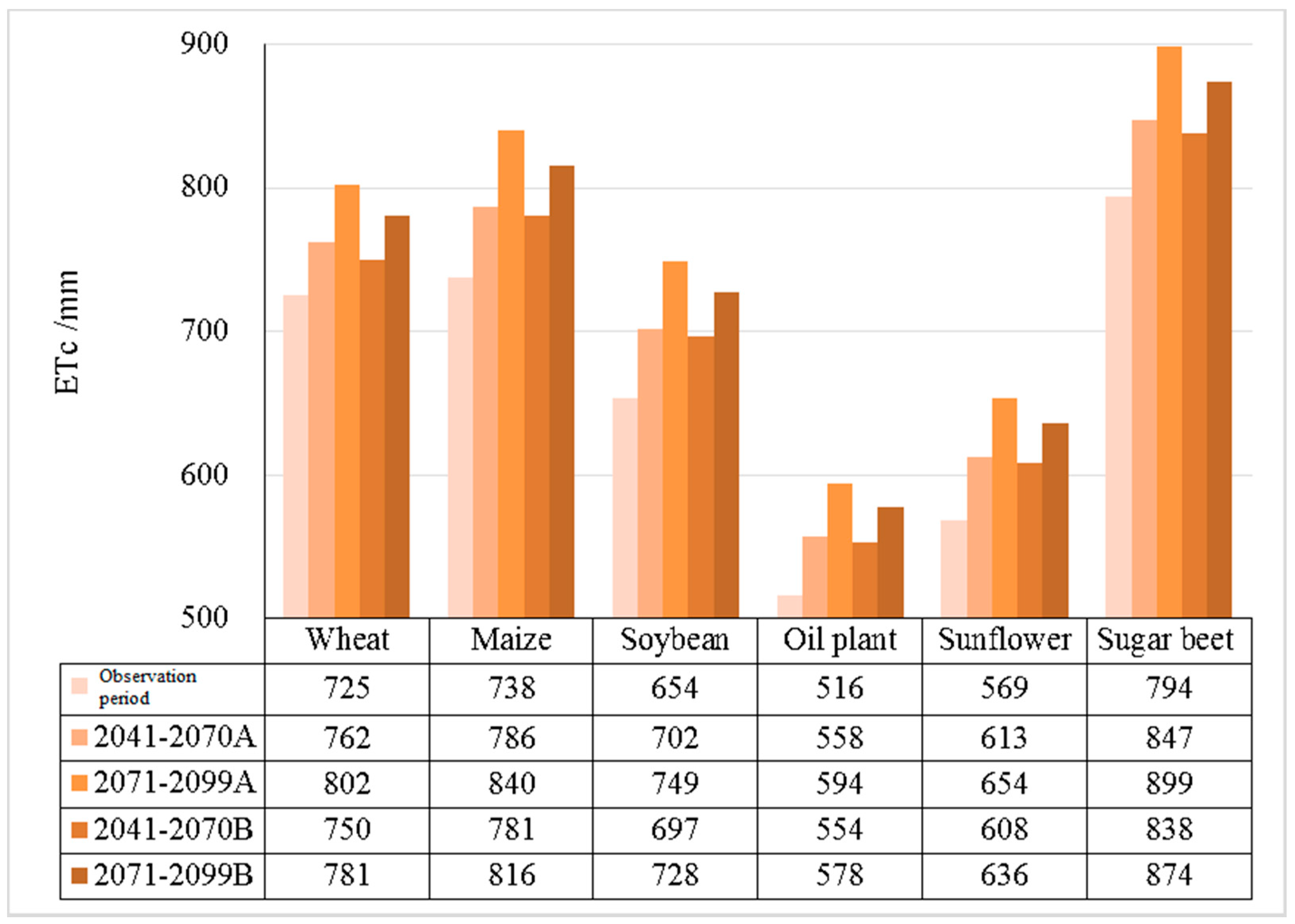
ETc is closely correlated with ET0, and indicates the amount of water that a type of plant needs during its growth season (i.e., CWR in this case). Figure 5 shows the ETc of six main crops grown in HID. Owing to the different growing periods and KC, the ETc of the six crops are different.
In terms of growth duration, maize is the longest among the six crops, followed by sugar beet. However, due to a higher KC, the ETc of sugar beet takes the first place, with 794 mm. The ETc of wheat, soybean, sunflower, and oil plant are reduced in turn, which is positively correlated with the growth duration of crops. The ETc of oil plant is the lowest with 516 mm, which is only 65% of that of sugar beet. The ETc of six crops all have the same temporal tendency as ET0, which means the future ETc would grow over time and the increment under scenario A2 would be more distinct. However, because of the difference in the growth season, the increment of ETc of the six crops are different, and when sorted in a descending order, it would be wheat, sugar beet, maize, soybean, sunflower, and oil plant. The increment of ETc of the six crops are the smallest during the years 2041–2070 under scenario B2, with 3.4–7.3%, and the largest during the years 2071–2099 under scenario A2, with 10.5–15.2%. So, the ETc of the six crops would grow as time passes, and the CWR in HID would increase.
3.4. Future Crop Water Irrigation Requirement in Potential Climate Scenarios
CIR is the quantity of additional water needed by crops via irrigation, beyond precipitation, to satisfy the crop’s growing period water requirements and guarantee their yield. A careful calculation of CIR is important in guiding the construction of water conservancy facilities and the management of water resources. This paper estimated the total CIR of the main crops grown in HID based on current sown area of crops.
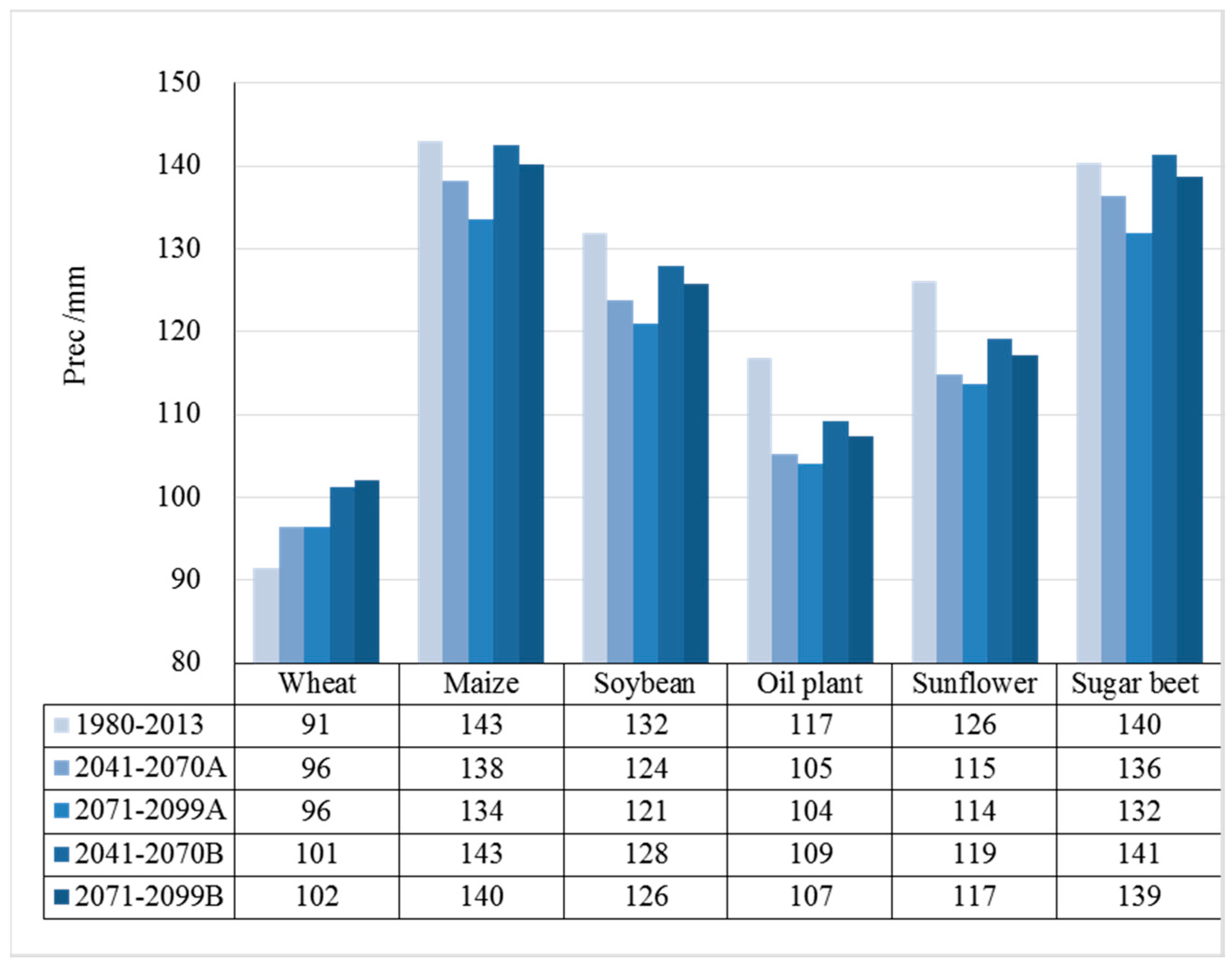
It can be seen from Figure 6 that the PE of 6 crops mainly show a downward trend, and the reduction is greater during the year 2071–2099. Because maize and sugar beet have similar plant and harvest dates (which means the length of their growth season are alike), the PE and reduction of PE during their growth season are almost the same, with 9 and 2 mm reduction during the years 2071–2099 under scenarios A2 and B2, respectively. Wheat ranks the third in the length of the growth season among these crops, but because of the earliest plant data which is in the dry season of the district, wheat has the lowest PE during the growth period, and even if it is the only crop whose future PE during the growth period would increase (about 5 mm under scenario A2 and 10 mm under scenario B2), its rank would not change. The length of the growth period of soybean, sunflower, and oil plant are reduced in turn, and so too are their PE during growth season. The reduction of PE of sunflower and oil plant during their growth season are the largest, with 12 mm under scenario A2 and 8 mm under scenario B2.
Due to the joint influence of increased ETc and decreased PE during the growth season, the future CIR would show an upward trend (Figure 7). The irrigation requirement of sugar beet is the largest among the six crops, and would show the largest increment. The increment would be 57 and 43 mm during the time period 2041–2070 under scenarios A2 and B2, respectively, and 113 and 81 mm during the time period 2071–2099 under scenarios A2 and B2, respectively. The PE of wheat during its growth period would increase, but the increment cannot compensate the increment in water demand of wheat, so the irrigation requirement of wheat shows an upward trend. The irrigation requirement of wheat would increase by 5–11% under scenario A2 and 2–7% under scenario B2.
Assuming the planting area of crops remain the same, this paper calculated the total CWR and CIR in HID during different time periods, and the results are shown in Table 3. The total CIR of HID is about 2.3 × 10⁹ m3 during the present stage, while under scenario A2 it would increase by 10.4% and 19.7% during the years 2041–2070 and 2071–2099 respectively, and under scenario B2, the increase during the years 2041–2070 and 2071–2099 would be 8.5% and 14.8%, respectively. Generally speaking, the changes of CWR and CIR have the same pattern, which is that the increment under scenario A2 is greater than under scenario B2, and greater during the years 2071–2099 than during the years 2041–2070. Furthermore, the increment would increase with the passage of time, which would bring HID an increasing pressure in water resource and a serious challenge in meeting the amount of water that crops need.
4. Discussion
According to the IPCC, it is almost certain that the global temperature and precipitation will rise in the future [2]. In the past few decades, researchers have pointed out that the temperature and precipitation have shown an increasing trend in Western China [28,29,30,31], and indicate that there is a chance that the climate in Western China will be warmer and wetter [32,33]. The results of this paper show that regardless of the climate scenario (A2 or B2), the temperature of HID would rise apparently and the future precipitation in HID would also increase, while the temperature increase would be greater under scenario A2 and the precipitation increase would be greater under scenario B2. The results indicate that the future climate of HID would be more hot and humid, which correspond with the results of others.
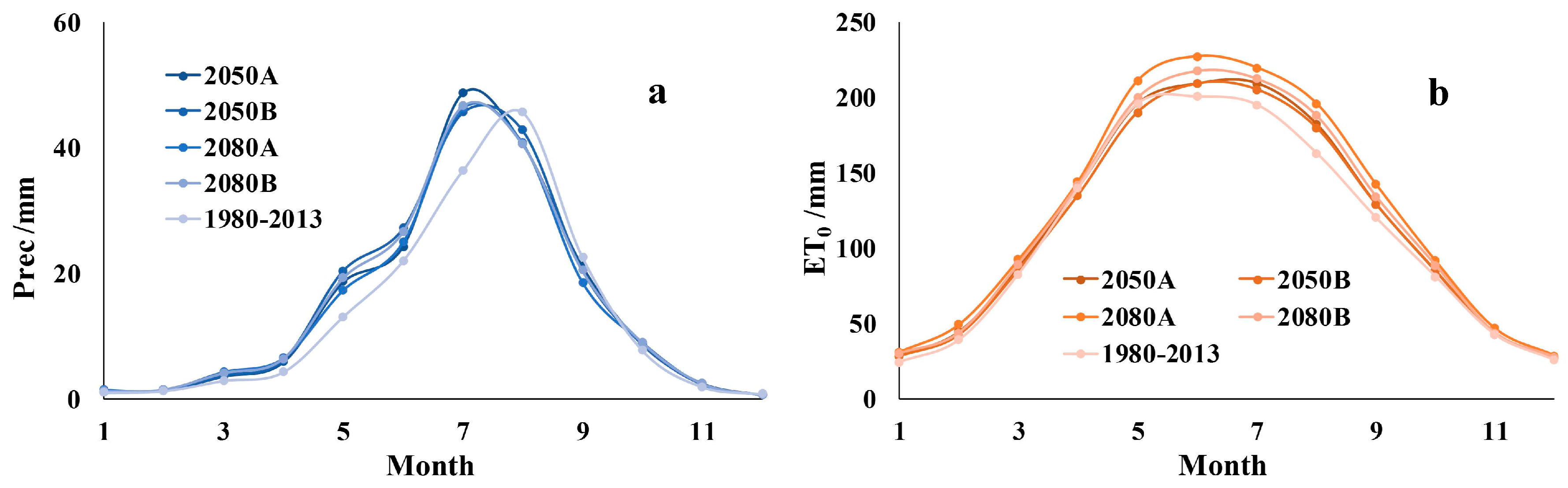
The results in Section 3.4 of this paper show that in spite of an increasing trend in annual precipitation, the PE during crop growth season would decrease. It can be learned from Figure 8a that the future precipitation mainly grows between March and July, and the month with largest precipitation would advance from August to July, and the future precipitation would be equal to or less than that of present after August. That is to say, the rainy season of HID would come earlier. However, the growing season of crops in HID is between April and September; furthermore, the growing season of sunflower and oil plant—whose sown area rank currently first among crops planted in HID—are mainly during June to September. The advance of rainy season leads to a discrepancy between growing season and rainy season, which means less precipitation during the crops’ growing period, and that is why the annual precipitation would increase while the PE of crops would decrease.
At the same time, the future ET0 would be greater (Figure 8b). Apart from the ET0 during the years 2041–2070 under B2 (whose value in April and May is slightly less than that of current day), the increase is mostly between April and September, which is the time period of the growth season of HID. The distribution of ET0 in every month under A2 and B2 have not much difference until the years 2071–2099, when the monthly average increase is 21 mm under A2 and 13 mm under B2. So, in the future, during the growth season of HID, the ET0 would be greater while PE would be less, which contributes to an increase in CIR and would bring an adverse condition to the agricultural production in HID.
Compared with B2, scenario A2 has a greater greenhouse gas emission, and the increment of temperature and ET0 under A2 would correspondingly be larger than under B2. With the increment of precipitation less than 20 mm, the pressure on agricultural production under A2 would be greater. It is required in the national comprehensive planning of water resources that by the year 2030, the irrigation water use efficiency should reach 0.60. So, calculations of the amount of water should be derived based on this regulation; the best condition is during the years 2041–2070 under B2, and 4.2 × 10⁹ m3 of water should be derived; the worst condition is during the years 2071–2099 under A2, and 4.6 × 10⁹ m3 of water should be derived. According to the water allocation set by the country, HID is allowed to derive 4 × 10⁹ m3 of water from the Yellow River, and the quota might be lower in the future. So, there would be a non-negligible gap between the water need and supply, which will threaten the agricultural production.
Some drawbacks of this study may be objects of future investigation. Although SDSM is a reliable tool in downscaling, it has no physical meaning, and the details for changes of parameters cannot be known. Many studies suggest that [34,35] ET0 has been changing periodically. This research is based on a 34-year period of time, which is not long enough to study the cycle of ET0 in HID, and if it does have a cycle at the present stage, whether or not the future ET0 will have the same cycle is not taken in to account.
5. Conclusions
The future sunshine hours of HID would be slightly lower, while the precipitation would increase. The average temperature would rise as time goes on, and the increase is greater under scenario A2. The spatial distribution of parameters would not change much. Hetao irrigation district will experience a warming and wetting climatic pattern in future.
ET0 is 1318 mm at present stage, and would increase by 7.14% and 4.48% during 2021–2099 under scenarios A2 and B2, respectively, and it increases predominantly throughout the growth period of crops. The main reason for the rise of ET0 is the rise of temperature. The spatial distribution of ET0 remains the same as the present stage, which reduces from west to east.
ETc and PE during crop growth season have a positive relationship with the length of the growth season of crops, but ETc shows an increasing trend while PE a decreasing one. The increment of ETc under A2 is greater than that under B2. The advance of the rainy season in the future is the major reason for the reduction of PE, and with the coefficient of the increasing of ETc and decreasing of PE, CIR during the years 2071–2099 would increase by 19.7% and 14.8% under scenarios A2 and B2, respectively.
Acknowledgments
This work is jointly supported by the National Key Research and Development Program of China (2016YFC0400201), National Natural Science Foundation of China (51409218), the Natural Science Basic Research Plan in Shaanxi Province of China (2016JQ5092; 2016KTZDNY-01-01) and the Fundamental Research Funds for the Central Universities (2014YB050).
Author Contributions
Pute Wu and Shikun Sun designed the study. Xiaobo Luan and Xiaolei Li did the literature search and data collection. Yubao Wang and Tianwa Zhou managed and analyzed the data. Suikun Sun and Tianwa Zhou drew the figures and wrote the paper. All authors discussed and commented on the manuscript.
Conflicts of Interest
The authors declare no conflict of interest.
References
- Solomon, S. Climate Change 2007—The Physical Science Basis: Working Group I Contribution to the Fourth Assessment Report of the IPCC; Cambridge University Press: Cambridge, UK, 2007. [Google Scholar]
- Stocker, T. Climate Change 2013: The Physical Science Basis: Working Group I Contribution to the Fifth Assessment Report of the Intergovernmental Panel on Climate Change; Cambridge University Press: Cambridge, UK, 2014. [Google Scholar]
- Schmidhuber, J.; Tubiello, F.N. Global food security under climate change. Proc. Natl. Acad. Sci. USA 2007, 104, 19703–19708. [Google Scholar] [CrossRef] [PubMed]
- Santis, B.; Dekkers, S.; Filippi, L.; Hutjes, R.W.A.; Noordam, M.Y.; Pisante, M.; Piva, G.; Prandini, A.; Toti, L.; van den Born, G.J.; et al. Climate change and food safety: An emerging issue with special focus on Europe. Food Chem. Toxicol. 2009, 47, 1009–1021. [Google Scholar] [CrossRef]
- Sun, S.K.; Wu, P.T.; Wang, Y.B.; Zhao, X.N.; Liu, J.; Zhang, X.H. The impacts of interannual climate variability and agricultural inputs on water footprint of crop production in an irrigation district of China. Sci. Total Environ. 2013, 444, 498–507. [Google Scholar] [CrossRef] [PubMed]
- FAO—Profile for Climate Change. Available online: http://www.fao.org/3/a-i1323e.pdf (accessed on 14 May 2009).
- Mehta, V.K.; Haden, V.R.; Joyce, B.A.; Purkey, D.R.; Jackson, L.E. Irrigation demand and supply, given projections of climate and land-use change, in Yolo County, California. Agric. Water Manag. 2013, 117, 70–82. [Google Scholar] [CrossRef]
- Saadi, S.; Todorovic, M.; Tanasijevic, L.; Pereira, L.S.; Pizzigalli, C.; Lionello, P. Climate change and Mediterranean agriculture: Impacts on winter wheat and tomato crop evapotranspiration, irrigation requirements and yield. Agric. Water Manag. 2015, 147, 103–115. [Google Scholar] [CrossRef]
- Wang, X.J.; Zhang, J.Y.; Ali, M.; Shahid, S.; He, R.M.; Xia, X.H.; Jiang, Z. Impact of climate change on regional irrigation water demand in Baojixia irrigation district of China. Mitig. Adapt. Strateg. Glob. Chang. 2016, 21, 233–247. [Google Scholar] [CrossRef]
- Wilby, R.L.; Dawson, C.W.; Murphy, C.; O’Connor, P.; Hawkins, E. The Statistical DownScaling Model—Decision Centric (SDSM-DC): Conceptual basis and applications. Clim. Res. 2014, 61, 259–276. [Google Scholar] [CrossRef]
- Diaz-Nieto, J.; Wilby, R.L. A comparison of statistical downscaling and climate change factor methods: Impacts on low flows in the River Thames, United Kingdom. Clim. Chang. 2005, 69, 245–268. [Google Scholar] [CrossRef]
- Wilby, R.L.; Dawson, C.W. The Statistical DownScaling Model: Insights from one decade of application. Int. J. Climatol. 2013, 33, 1707–1719. [Google Scholar] [CrossRef]
- Lee, E.J.; Kang, M.S.; Park, S.W.; Kim, H.K. Estimation of Future Reference Evapotranspiration Using Artificial Neural Network and Climate Change Scenario; American Society of Agricultural and Biological Engineers: Pittsburgh, PA, USA, 2010. [Google Scholar]
- Harmsen, E.W.; Miller, N.L.; Schlegel, N.J.; Gonzalez, J. Downscaled Climate Change Impacts on Reference Evapotranspiration and Rainfall Deficits in Puerto Rico. In Proceedings of the World Environmental and Water Resources Congress 2007: Restoring Our Natural Habitat, Tampa, FL, USA, 15–19 May 2007. [Google Scholar]
- Chun, K.P.; Wheater, H.S.; Onof, C. Projecting and hindcasting potential evaporation for the UK between 1950 and 2099. Clim. Chang. 2012, 113, 639–661. [Google Scholar] [CrossRef]
- Li, Z.; Zheng, F.L.; Liu, W.Z. Spatiotemporal characteristics of reference evapotranspiration during 1961–2009 and its projected changes during 2011–2099 on the Loess Plateau of China. Agric. For. Meteorol. 2012, 154, 147–155. [Google Scholar] [CrossRef]
- Sun, S.K.; Wu, P.T.; Wang, Y.B.; Zhao, X.N.; Liu, J.; Zhang, X.H. The temporal and spatial variability of water footprint of grain: A case study of an irrigation district in china from 1960 to 2008. J. Food Agric. Environ. 2012, 10, 1246–1251. [Google Scholar]
- Bai, G.; Zhang, R.; Geng, G.; Ren, Z.; Zhang, P.; Shi, J. Integrating Agricultural Water-saving Technologies in Hetao Irrigation District. Bull. Soil Water Conserv. 2011, 31, 149–154. [Google Scholar]
- Sun, S.K.; Wang, Y.B.; Liu, J.; Cai, H.J.; Wu, P.T.; Geng, Q.L.; Xu, L.J. Sustainability assessment of regional water resources under the DPSIR framework. J. Hydrol. 2016, 532, 140–148. [Google Scholar] [CrossRef]
- China Meteorology Administration. Available online: http://data.cma.cn/data/detail/dataCode/A.0029.0001.html (accessed on 22 April 2015).
- National Centers for Environmental Prediction. Available online: http://www.ncep.noaa.gov/ (accessed on 30 June 2015).
- Canadian Climate Data and Scenarios. Available online: http://www.cccsn.ec.gc.ca/?page=pred-hadcm3 (accessed on 10 May 2015).
- Met Office. Available online: http://www.metoffice.gov.uk/climate-guide/science/- science-behind-climate-change/hadley (accessed on 21 May 2015).
- Statistical Downscaling Model. Available online: http://co-public.lboro.ac.uk/cocwd/SDSM/data.html (accessed on 1 June 2015).
- Allen, R.G.; Pereira, L.S.; Raes, D.; Smith, M. Crop Evapotranspiration-Guidelines for Computing Crop Water Requirements—FAO Irrigation and Drainage Paper 56; FAO: Rome, Italy, 1998; Volume 300, p. D05109. [Google Scholar]
- Clarke, D.; Smith, M.; El-Askari, K. CropWat for Windows: User Guide; IHE: Oak Brook, IL, USA, 2001. [Google Scholar]
- Wilby, R.L.; Dawson, C.W.; Barrow, E.M. SDSM—A decision support tool for the assessment of regional climate change impacts. Environ. Modell. Softw. 2002, 17, 147–159. [Google Scholar] [CrossRef]
- Li, D.; Wei, L.; Cai, Y.; Zhang, C.; Feng, J.; Yang, Q.; Yuan, Y.; Dong, A. The present facts and the future tendency of the climate change in Northwest China. J. Glaciol. Geocryol. 2003, 25, 135–142. [Google Scholar]
- Wang, J.; Fei, X.; Wei, F. Further study of temperature change in Northwest China in recent 50 years. J. Desert Res. 2008, 28, 724–732. [Google Scholar]
- Wang, P.; Yang, J.; Zhang, Q.; He, J.; Wang, D.; Lu, D. Climate Change Characteristic of Northwest China in Recent Half Century. Adv. Earth Sci. 2007, 22, 649–656. [Google Scholar]
- Yu, S.; Lin, X.; Xu, X. The Climatic Change in Northwest China in Recent 50 Years. Clim. Environ. Res. 2003, 8, 9–18. [Google Scholar]
- Shi, Y.; Shen, Y.; Li, D.; Zhang, G.; Ding, Y.; Hu, R.; Kang, E. Disscussion on the present climate change from warm-dry to wram-wet in northwest China. Quat. Sci. 2003, 23, 152–164. [Google Scholar]
- Xu, Y.; Ding, Y.; Zhao, Z. Scenario of Temperature and Precipitation Changes in Northwest China Due to Human Activity in the 21st Century. J. Glaciol. Geocryol. 2003, 25, 327–330. [Google Scholar]
- Chen, X.; Lei, H.; Xu, J.; Huang, X.; Zhang, Z.; Hu, J.; Shang, C.; Yang, J. Spatial and Temporal Distribution Characteristics of Drought during Crop Growth Period in Guizhou Province from Climate Change Perspectives. J. Nat. Recourse 2015, 10, 1735–1749. [Google Scholar]
- Zeng, L.; Song, K.; Zhang, B.; Wang, Z.; Du, J. Spatiotemporal variability of reference evapotranspiration over the Northeast region of China in the last 60 years. Adv. Water Sci. 2010, 21, 194–200. [Google Scholar]
Figure 1.
The location of the Hetao Irrigation District.
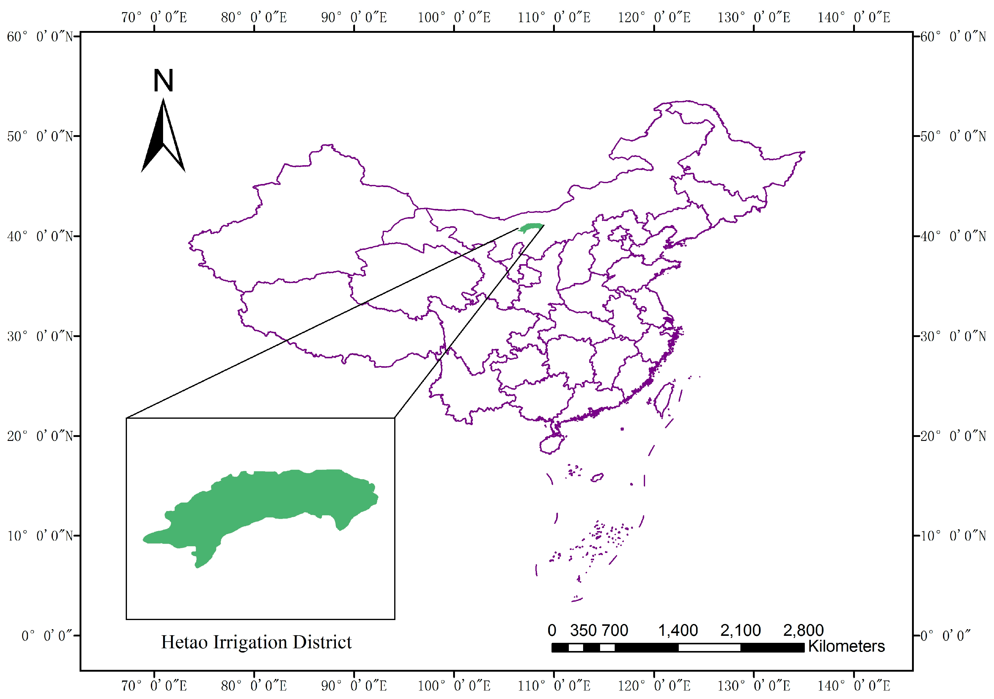
Figure 2.
The spatial distribution of the parameters during different time periods. (a–d) stand for average annual temperature (°C), sunshine hours (h), wind speed (m/s), and precipitation (mm), respectively.
Figure 2.
The spatial distribution of the parameters during different time periods. (a–d) stand for average annual temperature (°C), sunshine hours (h), wind speed (m/s), and precipitation (mm), respectively.

Figure 3.
The temporal change of ET0 during (a) 2021–2099 under scenario A2; (b) 2021–2099 under scenario B2; and (c) the present stage.
Figure 3.
The temporal change of ET0 during (a) 2021–2099 under scenario A2; (b) 2021–2099 under scenario B2; and (c) the present stage.
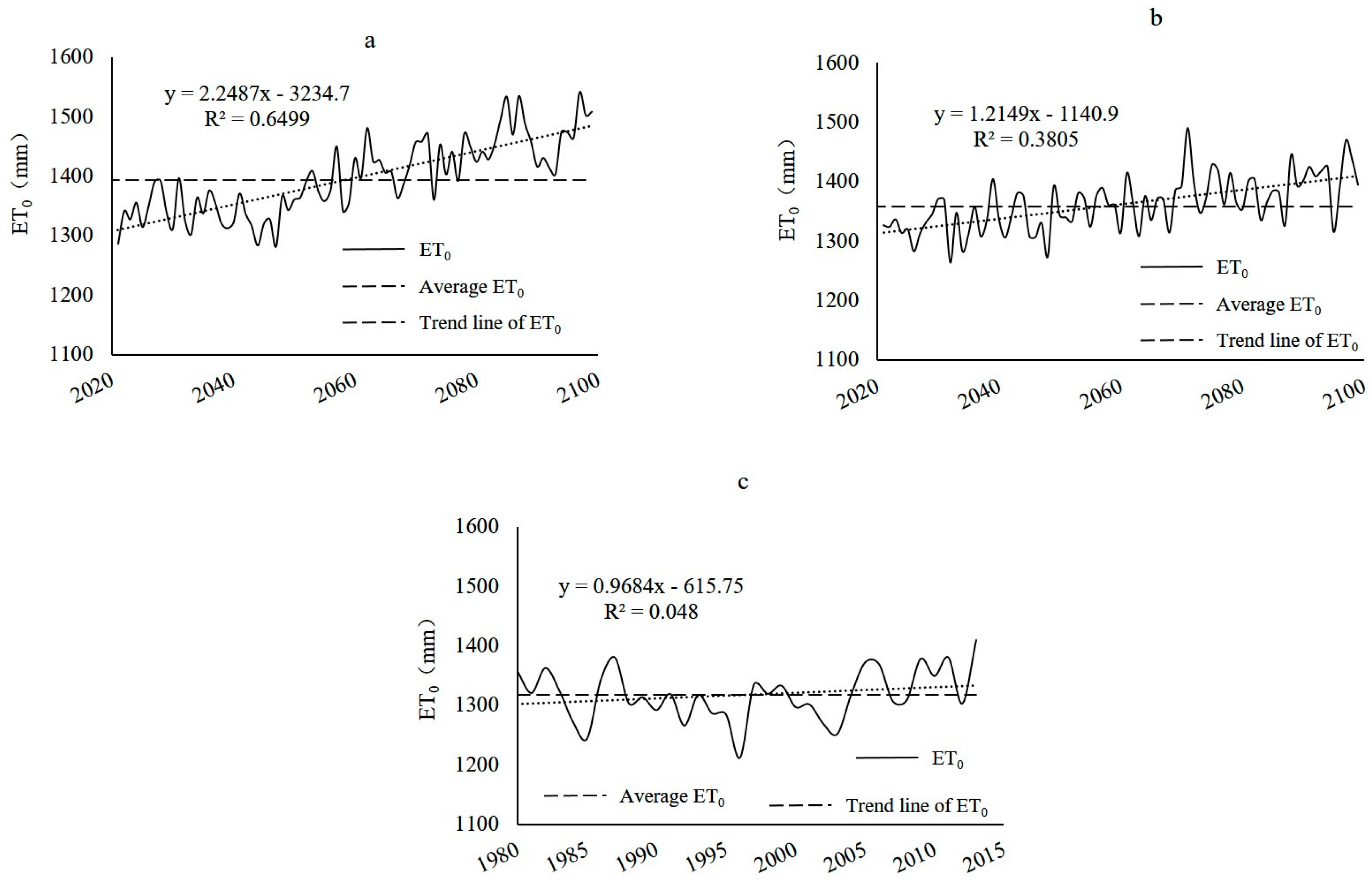
Figure 4.
The spatial distribution of ET0 during different time periods.
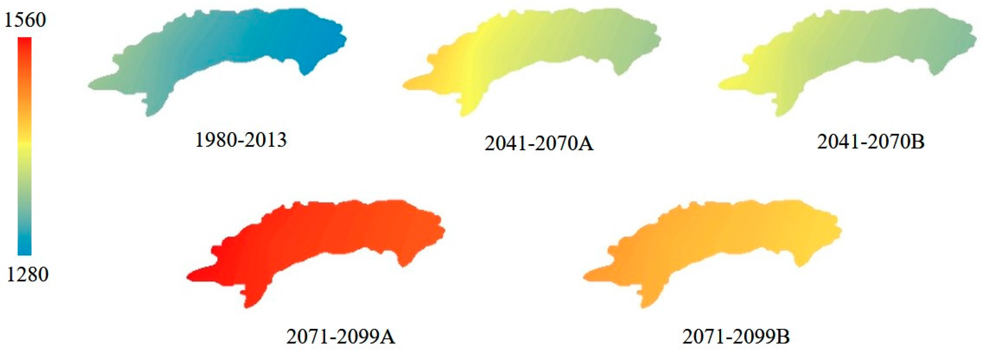
Figure 5.
ETc of different crops in different time periods.

Figure 6.
Effective precipitation (PE) during the growth period of different crops in different time periods.
Figure 6.
Effective precipitation (PE) during the growth period of different crops in different time periods.

Figure 7.
Crop irrigation Requirement (CIR) in different time periods.
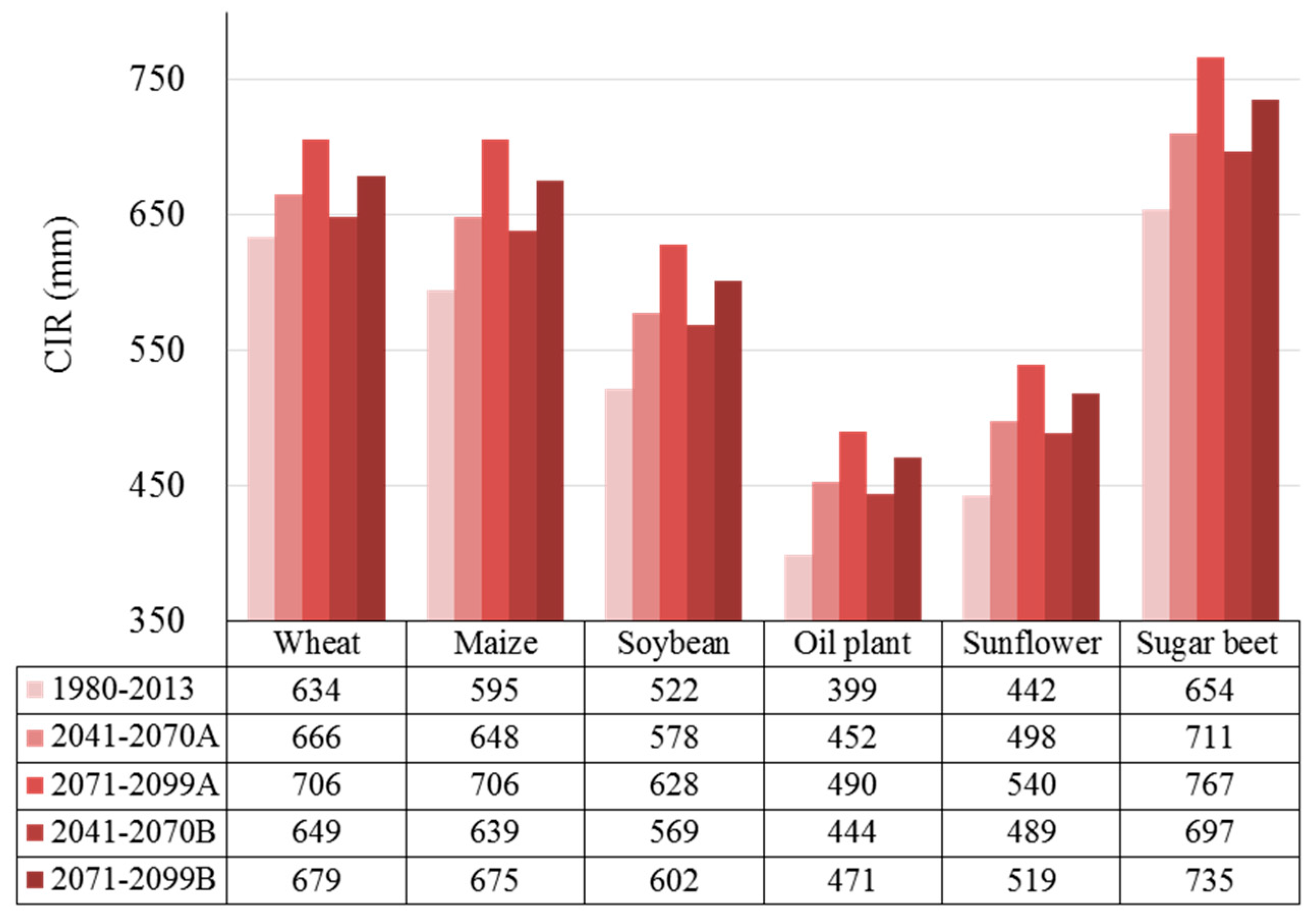
Figure 8.
Monthly average (a) precipitation and (b) ET0 in different time periods.


Table 1.
R2 and E of the average monthly value of the downscaled parameters.
| Parameters | A2 | B2 | ||
|---|---|---|---|---|
| R2 | E | R2 | E | |
| Tmin | 0.986 | 0.986 | 0.986 | 0.985 |
| Tmax | 0.997 | 0.997 | 0.997 | 0.996 |
| SH | 0.869 | 0.867 | 0.891 | 0.890 |
| WS | 0.916 | 0.854 | 0.923 | 0.853 |
| P | 0.967 | 0.929 | 0.974 | 0.943 |
| ET0 | 0.991 | 0.990 | 0.992 | 0.991 |
Notes: Tmin is the minimum temperature; Tmax the maximum temperature; SH the sunshine hours; WS the wind speed; P the precipitation; and ET0 the reference crop evapotranspiration.
Table 2.
The average value of parameters in different time periods.
| Time Period | Tmin (°C) | Tmax (°C) | SH (h) | WS (m/s) | P (mm) | RH (%) | |
|---|---|---|---|---|---|---|---|
| 1980–2013 | 1.15 | 14.02 | 8.61 | 2.46 | 159.10 | 48.25 | |
| A2 | 2041–2070 | 3.57 | 16.55 | 8.58 | 2.50 | 173.52 | 50.28 |
| 2071–2099 | 5.41 | 18.50 | 8.67 | 2.47 | 176.99 | 51.13 | |
| B2 | 2041–2070 | 3.20 | 16.03 | 8.50 | 2.49 | 180.53 | 50.46 |
| 2071–2099 | 4.21 | 17.12 | 8.56 | 2.46 | 178.81 | 51.07 | |
Notes: Tmin is the minimum temperature; Tmax is the maximum temperature; SH is the sunshine hours; WS is the wind speed; P is the precipitation; and RH is the relative humidity.
Table 3.
CWR and CIR of HID in different time periods (×109 m3).
| Time Period | 1980–2013 | 2041–2070A | 2041–2070B | 2071–2099A | 2071–2099B |
|---|---|---|---|---|---|
| CWR | 2.905 | 3.111 | 3.087 | 3.315 | 3.223 |
| CIR | 2.318 | 2.560 | 2.516 | 2.774 | 2.660 |
Notes: CWR is crop water requirement; CIR is crop irrigation requirement and HID is Hetao irrigation district.
© 2017 by the authors. Licensee MDPI, Basel, Switzerland. This article is an open access article distributed under the terms and conditions of the Creative Commons Attribution (CC BY) license (http://creativecommons.org/licenses/by/4.0/).
Share and Cite
MDPI and ACS Style
Zhou, T.; Wu, P.; Sun, S.; Li, X.; Wang, Y.; Luan, X. Impact of Future Climate Change on Regional Crop Water Requirement—A Case Study of Hetao Irrigation District, China. Water 2017, 9, 429. https://doi.org/10.3390/w9060429
AMA Style
Zhou T, Wu P, Sun S, Li X, Wang Y, Luan X. Impact of Future Climate Change on Regional Crop Water Requirement—A Case Study of Hetao Irrigation District, China. Water. 2017; 9(6):429. https://doi.org/10.3390/w9060429
Chicago/Turabian StyleZhou, Tianwa, Pute Wu, Shikun Sun, Xiaolei Li, Yubao Wang, and Xiaobo Luan. 2017. "Impact of Future Climate Change on Regional Crop Water Requirement—A Case Study of Hetao Irrigation District, China" Water 9, no. 6: 429. https://doi.org/10.3390/w9060429
Note that from the first issue of 2016, this journal uses article numbers instead of page numbers. See further details here.