
System Reliability Evaluation in Water Distribution Networks with the Impact of Valves Experiencing Cascading Failures


1
Department of Construction Management, School of Economics and Management, Beijing Jiaotong University, Beijing 100044, China
2
Beijing Center for Industrial Security and Development Research, Beijing 100044, China
3
College of Geophysics and Information Engineering, China University of Petroleum, Beijing 102249, China
*
Author to whom correspondence should be addressed.
Water 2017, 9(6), 413; https://doi.org/10.3390/w9060413
Submission received: 31 March 2017
/
Revised: 8 May 2017
/
Accepted: 5 June 2017
/
Published: 9 June 2017
Abstract
:Water distribution networks (WDNs) represent a class of critical infrastructure networks. When a disaster occurs, component failures in a WDN may trigger system failures that result in larger-scale reactions. The aim of the paper is to evaluate the evolution of system reliability and failure propagation time for a WDN experiencing cascading failures, and find the critical pipes which may reduce system reliability dramatically. Multiple factors are considered in the method such as network topology, the balance of water supply and demand, demand multiplier, and pipe break isolation. The pipe-based attack with multiple failure scenarios is simulated in the paper. A case WDN is used to illustrate the method. The results show that the lowest capacity gets stronger when a WDN is short of supply, becoming the dominant factor that decides the evolution of system reliability and failure propagation time. The valve ratio (VR) and system reliability present a flattened S curve relationship, and there are two turning points in VR. The critical pipes can be identified. With the fixed 5% valves, a WDN can improve system reliability and resist cascading failures effectively. The findings provide insights into the system reliability and failure propagation time for WDNs experiencing cascading failures. It is proven to be useful in future studies focused on the operation and management of water services.
1. Introduction
Our modern society is highly dependent on critical infrastructures such as communication, power, transportation, and water supply systems. Water distribution networks (WDNs) collectively form a key component of the supply system. The stability and reliability of such systems are significant factors in ensuring public safety and normal city operations. However, failure is inevitable during the lifetime of a WDN, which can reduce the integrity of the supply system and interrupt its continuous operation [1]. It is vital to monitor and detect the worst failure scenarios.
A WDN can be represented as a spatially organized network consisting of nodes (e.g., reservoirs, tanks, and consumers) and links (e.g., pipes, pumps, and valves) [2,3]. As time passes by, WDNs have been upgraded to form a complex and nonlinear network structure requiring a continuous reliable design and optimal controls for random user demand.
Given its correlation with various geographic distributions, WDNs are particularly sensitive to disturbances caused by natural and man-made disasters [4]. Damage to key components of a WDN may result in property loss and even impact overall socioeconomic development and human life. In studies on network attacks [5,6,7], cascading failures have become an increasingly vital issue in network security. More specifically, a cascading failure is a process of conductive failures [8]. When a network encounters natural or man-made disasters, i.e., an attack on the network, the abnormal event may spread through the entire system, often resulting in a large-scale chain reaction and secondary failures. Such failure scenarios can trigger multiple unfavorable impacts on a WDN. They reduce WDN reliability dramatically and result in unexpected consequences.
Network attacks can be categorized into either random or intentional attacks [9]. A random attack indicates randomly occurring damage to a certain component of a WDN, whereas an intentional attack implies an attack on a certain component with a particular selection strategy. In studies of attacks involving cascading failures, Albert et al. [10] found that scale-free networks provide a high level of robustness versus random disturbances, but extreme vulnerabilities to intentional attacks. Since the urban infrastructure network is associated with a geographic spatial distribution, natural disasters do not typically fall into the random attack category. As an example, human populations, telecommunications, transportation infrastructure, and finance centers may all be distributed around earthquake-prone regions, such as the Pacific Rim [11]. According to studies on urban infrastructure network attacks (e.g., [8]), infrastructure networks are usually able to withstand random failures; however, given an intentional attack, network components with higher loads are more likely to be targets and trigger cascading failures.
Given the above, it is very important to study cascading failures in WDNs facing intentional attacks. The cascading failures can be categorized into multiple failure scenarios. Single failure in WDNs has been wildly discussed in the literature [12,13,14], and few studies have focused on multiple failure scenarios. Multiple failure scenarios mean more than one pipe failure at a time. Gheisi et al. [15] indicated that a WDN was in multiple failure scenarios at 78.5%. Berardi et al. [16] stated that multiple mechanical failures can result in abrupt modifications of WDN topology and water supply capacity. Gheisi et al. [17] reported very little attention has been paid to multiple failure scenarios due to the large computational workload was required. Laucelli et al. [18] emphasized that multiple failures was the most critical scenario. They analyzed the consequences of multiple pipe failures in WDNs to earthquakes. The cascading failures in WDNs involve several pipe failures at a time, and this situation may lead to more pipes failing in the next failure step. A WDN is reliable at a single failure state but may be unreliable when multiple failures are considered. To check cascading failures in a WDN, the multiple failure scenarios need to be embedded in the reliability simulation.
Many studies have focused on analyzing WDNs using graph theory. Yazdani et al. [19] proposed that WDNs can be viewed as spatially organized networks, thus giving researchers the opportunity to consider more complex network properties, such as network structure, efficiency, robustness, and vulnerability, to evaluate WDNs. Yazdani et al. [2] focused their research on an urban WDN, quantifying both redundancy and failure tolerance. They found it effective to analyze using the network structure, but inferior to assess resilience and robustness against a disaster and disturbances. Hawick [20] argued that WDNs have developed into highly complex networks after numerous optimizations and design changes. Betweenness can be used to sort WDNs’ component reliability and the influence of component failure was analyzed. However, studies that are focused on reliability using graph theory, which specifically consider cascading failures, are still rather limited. Yazdani et al. [21] evaluated and quantified the ability of WDNs to withstand cascading failures by applying a statistical analysis of graph theory and a complex network. Sitzenfrei et al. [22] established a cascade risk map using a geographic information system (GIS), proposing that ignoring the cascade effect leads to significant underestimations of risk. Therefore, assessing the impact of the cascade effect is crucial to WDN risk analysis.
In the above studies, the analysis of WDN performance was implemented based on the network topological structure; such methods are classified as topology-based methods. Unfortunately, these topology-based methods ignore node heterogeneity. Instead, these methods primarily capture topological features, paying little attention to the function of supply nodes, trans-shipment nodes, and demand nodes [23,24]. Therefore, topology-based methods alone do not have access to sufficient information regarding flow performance of real system infrastructures [25]. To assess the reliability of a WDN, the topology-based methods should be analyzed with firm hydraulic knowledge [26].
In general, WDN system reliability while facing failures depends on two key factors, i.e., the topological structure and the balance of water supply and demand. We have described the former above, whereas the latter is derived from service delivery. In the method classification, the service that is made and delivered is classified as flow-based methods. Hence, unlike the purely topological methods, in this paper, we apply the flow-based approach. We analyze both the redistribution of water hydraulics and updates to the network structure. To present a more practical model, we adopt uncertainties such as pressure, flow, water demand, and valve ratio in our simulations.
In addition to the above, the capacity in the cascading failure model is described as the maximum load that a given node can bear. The capacity Ci is thereby proportional to its initial load Li, i.e., Ci = λi. Li, where λi > 1, is the tolerance parameter. Note that this model has been used in a complex network and power grid evaluation [5,8,9,25,27,28,29].
In WDNs, the nodal load can be expressed as nodal pressure [30]. Here, nodal pressure should be neither too high nor too low. High pressure can lead to a pipe breaking, whereas low pressure can result in flow reductions. Therefore, capacity is limited in two ways, i.e., a maximum capacity for avoiding pipe leakage or aging pipe bursts and a minimum capacity for effectively maintaining water supply. Thus, nodal capacities can change as the water supply system runs for long periods of time. As an example, after long-term utilization, the pressure tolerance decreases with aging components, and extra pressure assisted devices are used to enhance the bearing ability with the pressure deficiency problem. In this paper, in contrast to the original cascading failure model, the maximum and minimum capacities are both considered as dynamic constraints in evaluating WDN reliability. We thereby model the dynamic process of WDN reliability facing cascading failures.
More specifically, in this paper, we evaluate WDN from two perspectives, i.e., system reliability and failure propagation time. Here, system reliability is defined as the probability of satisfying user demand with an appropriate pressure given various possible failures at any given time. Furthermore, the failure propagation time describes the time that cascading failures transmit and spread through a WDN. The pipe-based cascading failures, i.e., the multiple failure scenarios, are simulated in the paper. Multiple factors are considered in the method such as network topology, the balance of water supply and demand, demand multiplier, and pipe break isolation. A quantitative investigation of the system reliability and failure propagation time of WDNs facing cascading failures and maintaining a balance of water service is provided. One WDN extracted from a real system is presented as a numerical example to illustrate our analysis. Through the simulations, the dynamic process of system reliability and failure propagation time with the highest and lowest pressure constraints are conducted. The evolution of the system reliability and valve ratio is discussed. Further, the critical pipes and the fixed valve locations can be obtained. The WDN system reliability is improved with the valve adjustment scheme. Our findings provide insight into the reliability of WDNs given cascading failures. It is proven to be useful for future studies into the operation and management of water services.
2. Pipe-Based Cascading Failure Model
2.1. Evaluation
WDN is evaluated by the system reliability and failure propagation time, each of which is described below.
2.1.1. Reliability
There are two types of WDN reliability, i.e., mechanical reliability and hydraulic reliability [31]. Mechanical reliability focuses on network topology analysis and connectivity of the system given a failure, but ignores the ability of the system to effectively supply water. Hydraulic reliability refers to the ability of the system to meet the requirements of water flow and pressure and focuses on the failures caused by changes in demand, aging pipes, and an insufficient water supply, all of which cause WDN to fail to meet the water demand. In some studies, these are merged to evaluate WDNs [13,32,33].
In this paper, system reliability is defined as the probability that water is successfully supplied to customers during a failure period [34]. Mathematically, system reliability is expressed as the ratio of the total actual water demand versus the total required water demand given different failures.
where Rsys represents system reliability, and m represents the number of nodes in the given WDN, Qk,t,act is the actual demand delivered to the kth node at time step t, and Qk,req is the required demand at the kth node.
2.1.2. Failure Propagation Time
The time during cascading failures with different initial failures in a WDN is typically not the same. The time step t is introduced to describe the load redistribution process during cascade propagation. First, t = 0 represents the initial state, i.e., a point in time when no failures occur. Next, t = 1 describes a certain component failure that causes the network topology and load to change. After this, t = 2 describes secondary failures. Throughout this process, new failure nodes and pipes may appear owing to load redistribution. If the redistributed load exceeds the nodal capacity, the node is recognized as a new failure node. The outflow pipes connected with the failure node are recognized as new failure pipes. Finally, t = 3, 4, 5… describes the cascading propagation process. At each time step, new failure nodes and pipes appear.
The cascading propagation process stops when no new failure components are generated. The failure propagation time is selected as the time step when the cascading propagation stops. It describes the time that cascading failures transmit and spread through WDN.
2.2. Representation of WDN
A WDN can be represented as a directed graph that represents water flowing in a certain direction. In general, a directed graph consists of a set of nodes and one-way links [35]; here, we represent the intersections of pipes, tanks, and reservoirs as nodes and pipes, valves, and pumps as links. Overall, the directed graph describes the network connectivity, which is recorded using incidence matrix A. An incidence matrix describes the relationship between nodes and links. The m rows of N represent the nodes, whereas the n columns represent the links. For each cell A(i, j), if the cell’s value is set to 1, node i is the initial point of directed link j, whereas a value of −1 represents node i as the terminal point of link j; otherwise, 0 is assigned.
The node-link incidence matrix B is used to describe the relationship between nodes, pipes, and valves. The rows of B represent the nodes while the columns represent the pipes or valves. Values of B can be 0, 1, or −1. The elements in B can be expressed as
With these link-node representations A and B, WDN topologic information can be recognized and processed via the computer.
2.3. Capacity
The effect and reaction of a WDN experiencing cascading failures can be observed by the network capacity and load. Here, capacity represents the extra network flow that a component can bear during a failure, and load represents the network flow passing through the component. In previous studies, researchers have used topological metric parameters, e.g., betweenness or degree, to approximate the network load [36]; however, a WDN is operated with a balance in water supply and demand. Pressure in a WDN should be neither too low nor too high. With this condition, the nodal service pressure Pser is adopted as the initial load [30]. Here, Pser ensures the supply and demand requirements under normal operating conditions. In this paper, load is different from that of topology-based methods in that we make use of both water hydraulics and topological features.
Attacks on pipes lead to perturbations in WDN. Such a perturbation is a small unusual change that may trigger flow redistribution. If the redistributed load exceeds its capacity, new failures occur downstream. Cascading failures are a series of failures caused by flow redistributions after component failures. In general, capacity determines whether or not each failure occurs.
Capacity is therefore an important factor in a WDN. With cities expanding, WDNs are often expanded based on their original scale. Increases in population and industry cause dynamic changes in water demand. These requirements lead to peak usage and trough usage each day. With such variations in demand, node pressures deviate from their original design value and typically keep changing. For WDNs that exist for long periods of time, it is necessary to consider changes in node pressure.
We define the highest capacity of nodal pressure as
where Pk,ser is the service pressure at the kth node. Pk,max represents the highest capacity of cost and aging water system components, with α included as a tolerance parameter greater than 0. Essentially, α represents the extra pressure that a node in the given WDN can bear. The larger α we use here, the larger the capacity range will be, indicating that the safe range of the given node is larger.
After a failure occurs, there are three potential patterns for nodal pressure to follow; these are the following: (1) the node receives extra pressure from the broken node; (2) the node pressure remains the same; and (3) the node pressure is lower than the initial load. Lower pressure usually leads to interruptions in supply.
Considering this third potential pattern, we define the lowest capacity of nodal pressure as
where Pk,min represents the lowest capacity of carrying pressure within which the shortage of supply is tolerated. Here, 1 ≥ β ≥ 0 is a tolerance parameter. When α and β have a consistent change direction, there are minimal or no changes in the probability of node failure.
2.4. Pressure-Driven Analysis
Redistributed loads can be calculated using hydraulic simulations; we adopt a pressure-driven analysis, which is one of the most recent WDN modeling methods that can effectively avoid negative pressure given a failure [37]. To analyze the redistributed load, we express some necessary factors below.
Water demand is a dynamic factor in a WDN. In general, changes in water demand depend on the daily activities of consumers [38]. The required demand describes the amount that consumers use, which can be expressed as
where Qk,req is the required demand at the kth node, DMk is the nodal demand multiplier (i.e., DM) at the kth node, which changes dynamically throughout the day, and Qk,base is the base demand at the kth node.
Unfortunately, supply cannot always meet the requirements of demand. Actual demand describes the actual amount that consumers can use. To obtain the actual demand, Wagner’s model is used to calculate nodal demand for networks with component failures [39,40]:
where Pk,t is the computed pressure at the kth node at time step t.
EPANET (2.0, Environmental Protection Agency, Cincinnati, OH, USA) is used to implement our hydraulic simulations [41]. To realize the pressure-driven analysis described above, MATLAB 2010a is used to call EPANET 2.0 Toolkits dynamic link library to simulate cascading failures. The nodal pressure is calculated by EPANET 2.0 Toolkits, while the actual demand delivered to customers under abnormal conditions is conducted by MATLAB 2010a.
2.5. Rules for Pipe Break Isolation
A WDN contains valves, which allows it to isolate segments to limit the effect of a pipe break. Hence valves are a crucial factor in evaluating the reliability of a WDN under cascading failures. There are a numbers of studies that focus on identification of the segments [42,43,44]. The method of pipe break isolation is adopted by Zhuang et al. [45].
This method contains three steps. After a pipe break, the valves near the failure pipe are firstly recognized. The depth-first search (DFS) method [46] is used to locate the nearest valves. The direct isolated segments with nodes and pipes can be obtained. The unintended isolation may also happen due to some nodes that are disconnected with all sources by the closing valves. The topological detection is then carried out to determine the redundant valves. The redundant valves are located between the direct and unintended isolation. The final isolated segments are surrounded with valves except the redundant valves.
For hydraulic analysis software such as EPANET 2.0, it cannot perform the analysis if a node is not connected to the sources but still has water demand. Node demands are updated after topological detection. For nodes within the isolated segments, their nodal demands are set to zero. For nodes on the edge of isolated segments, it is assumed that their nodal demands are reduced by the rate of isolated links and total links.
2.6. Pipe-Based Cascading Failures
Intentional attacks are adopted in this paper. As previously noted, trigger conditions for failures are typically divided into random attacks and intentional attacks [9]. Random attacks target network components selected at random, whereas intentional attacks target network components using a strategy. If the network information is unknown, components can only be attacked randomly. Often ignored, in real systems, the relative importance of each component may be different from one another. When network information can be entirely obtained or only in part, the network may be broken more easily if the priority is given to key components.
In general, real systems are able to withstand random failures; however, in contrast, intentional attacks are likely to trigger cascading failures that then lead to large-scale consequences and secondary failures. Moreover, load-based intentional attacks are more likely to trigger an overall cascading failure. Despite its high tolerance, damage to a high capacity node can still result in failures of the associated components.
Intentional attacks can start from the nodes or pipes. In this paper, we focus on the pipe-based attack. If a pipe is broken, the first step is to search the nearest valves and determine the isolation segments. The network topological structure has changed according to the closed valves, and the node demand is also adjusted to perform the hydraulic analysis.
The hydraulic failure is not necessarily related to a network mechanical failure even if the network is correctly designed on average. However, WDNs have uncertainties of spatial-temporal fluctuations in the flow demand, of pipe roughness, and of reservoir levels. These uncertainties can affect the network and lead to the hydraulic failure. As discussed in Darvini et al. [47], when the supply request is at the minimum, the uncertainties only lead to a small increase of hydraulic failure with respect to that due to pipe burst, and the nodal reliability is dominated by the mechanical failure only. In contrast, by increasing the supply request, the nodal reliability is strongly affected by the uncertainties. The uncertainties increase the hydraulic unavailability for the medium and maximum request. Hence, after the mechanical failure of the pipe, the network flow is redistributed. The nodal pressure generally decreases. Somewhere the nodal pressure may increase, e.g., due to a reduction of the water demand and consequently of the head losses. Nodes fail when the pressure falls below the lowest capacity, due to (i) mechanical unavailability; or (ii) uncertainty related to the distribution of nodal demand and to the pipe roughness. In both cases, cascade failures may take place. It is noted that the node-based attack starts from a certain node. It has a similar simulation to the pipe-based attack. Hence in this paper, we focus on the pipe-based attack.
2.7. Assumptions and Algorithm
2.7.1. Assumptions
1. Nodes. Each demand node has three states: operation, failure, or reduction of service. A node is operational if its nodal pressure is neither higher than the highest capacity nor lower than the lowest capacity. The downstream pipes which connect with a failure node need to be isolated by valves. The reduction of service means that the nodal pressure is higher than the minimum pressure, but lower than the service pressure. The amount of water demand is available but supplied at a reduced level.
2. Pipes. Each pipe has two states: operation or failure. A pipe is operational if water can flow smoothly. A failure pipe is isolated by the valves.
3. Valves: the N valve rule indicates that one pipe can be isolated by two valves at its opposite nodes. However, a real WDN can hardly achieve this condition. The maximum number of valves in a WDN is 2n (n is the total number of links). Define the valve ratio (VR) as the ratio of actual valves and maximum valves. It is assumed that valves are located randomly by the valve rate.
4. Node demand. Node demand is equally distributed among the links connected to the node. After a failure occurs, the node demand is updated according to the detection of isolation segments.
5. Multiple failure scenarios. A certain pipe failure may lead to multiple failures. It is assumed that several pipes are in failure at a time according to the topological and hydraulic analysis.
6. Terminating condition. Two terminating conditions are set for cascading failures: (1) no other pipe fails; (2) all valves are closed.
2.7.2. Algorithm
Algorithm 1 summarizes our cascade propagation process. First, we load the basic information of the WDN; here, the basic information includes topology information, i.e., the incidence matrix, and water information, i.e., the nodal elevation, base demands, pipe diameters, lengths, and roughness coefficient.
Second, we run the hydraulic simulation software to obtain the service pressure under normal conditions. This is a conventional definition, due to the fact that a WDN system is usually operating in a normal range of pressure and flow conditions. We use service pressure as the initial load. Nodal capacity is then calculated using Equations (3) and (4). For the initial step, t = 0 represents the obtained normal conditions.
Third, we set four parameters before we truly start our cascade simulation. More specifically, we set the demand multiplier DM to analyze the supply–demand relationship. Tolerant parameters α and β are used to calculate the highest capacity and lowest capacity, respectively; here, α and β evaluate the safe range in which the load can change. These three parameters are set according to the given WDN conditions. The last parameter is the valve ratio VR. It states how many valves are set in WDN. The locations of the valves are random.
Fourth, we simulate the pipe-based attack. Each pipe in the WDN is simulated separately as the attack target. Therefore, t = 1 represents the time at which the ith pipe fails. For each pipe, after a failure occurs, the failed pipe is isolated by the valves.
Next, we compute the isolated, hydraulic, and topological analyses. The isolated analysis searches for the isolation segments which combine the direct and unintended isolation. The WDN topological structure is then changed and the node demands are updated according to the isolation segments.
The hydraulic analysis simulates the status of the WDN and obtains the pressure and flow. If the nodal pressure is lower than the lowest capacity, the node is recognized as a secondary failure due to the node that cannot meet the demand. If the mean nodal pressure is higher than the highest capacity, the node maybe hydraulically failed due to the uncertainties in the WDN. For the operational node, the actual demand is calculated according to the updated pressure by using Equation (6). For the nodal pressure lower than the lowest capacity, the actual demand is set to zero.
Our topological analysis updates the network topology structure in two steps. First, we update the incidence matrix according to the updated flow. Second, the outflow pipes associated with the failed node are regarded as new failure pipes.
We repeat these three analyses until the network reaches a new stable state, i.e., a state in which no new pipe or node failures occur. The system reliability is then calculated using Equation (1), and the failure propagation time is obtained via the iteration.
After all pipes are simulated as attack targets, network reliability can then be calculated. Note that we use average values for our final network reliability assessments to avoid fluctuations in each pipe or node cascade simulation. More specifically, for pipe-based attacks, the network system reliability is the average for the given n pipes; likewise, the network failure propagation time is the average for the given n pipes’ failure propagation time.
| Algorithm 1. Simulation of cascade propagation in a WDN | |
| 1: | Load the basic WDN information. |
| 2: | Calculate the initial load and capacity. |
| 3: | Set t = 0 |
| 4: | Set simulation parameters DM, α, and β. |
| 5: | Case DM |
| 6: | for α = 0 → maximum do |
| 7: | for β = 0 → maximum do |
| 8: | for i = 1 → n (for pipe-based attack) do |
| 9: | Set t = 1. |
| 10: | while new failures exist do |
| 11: | Set t = t + 1. |
| 12: | Perform isolated analysis. Update topological structure and node demand. |
| 13: | Perform hydraulic analysis. Update loads after redistribution. |
| 14: | Perform topological analysis. Update topology structure after redistribution. |
| 15: | end while |
| 16: | Calculate system reliability and failure propagation time. |
| 17: | end for |
| 18: | end for |
| 19: | end for |
| 20: | end Case |
| Calculate network reliability. | |
3. Results
3.1. Case Study
To clarify the proposed pipe-based cascading failure model and assess the roles of different parameters involved in the model, a WDN reported by Islam et al. [48] is applied and analyzed as an example. The network topological structure, nodal elevations, base demands, pipe diameters, lengths, and Hazen-Williams roughness are shown in Figure 1. This water network is constructed using 2 reservoirs, 25 nodes, and 40 pipes. Nodes 26 and 27 are elevated reservoirs with total heads of 90 and 85 m, respectively. The total pipe length is 19.5 km, with pipe lengths ranging from 100 to 680 m. Pipe diameters vary from 200 to 700 mm, and the base demands vary from 33.33 to 133.33 L/s. The Hazen-Williams formula is used to calculate head loss.
Initially, the water network is in balance, i.e., the water supply meets the requirements of demand, and no failures have occurred. The nodal pressures are calculated with EPANET 2.0. The calculation results are shown in Table 1.
In our simulation, there are four parameters that must be set, i.e., DM, α, β, and VR. Here, water demands dynamically change throughout a given day according to consumer use. In our present work, we chose four potential situations that may occur in terms of water usage, i.e., DM values of 0.5, 1.0, 1.5, and 2.0.
According to Equations (3) and (4), tolerant parameters α and β are used to calculate the highest and lowest capacities, respectively. The value of the tolerant parameters depends on the WDN. To cover all possible conditions, the value of α and β are set within the range of 0 to 0.5, with an iterative step of 0.05.
3.2. System Reliability Evolution with Fixed VR
VR is fixed at 100% to study the evolution of system reliability and duration given cascading failures.
Table 2 shows the maximum value of system reliability (MVSR) results with different DMs. Here, the reduction is calculated as the difference between the previous DM and the current DM. From the table, the MVSR decreases with increases in DM. Further, the MVSR changes slightly as DM < 1, i.e., the reduction between DM = 0.5 and DM = 1.0 only drops 0.26%. In contrast, the MVSR decreases dramatically as DM > 1. The reduction between DM = 2.0 and DM = 1.5 is three times larger than the reduction between DM = 1.5 and DM = 1.0. It indicates that the shortage of supply accelerates the influence of cascading failures.
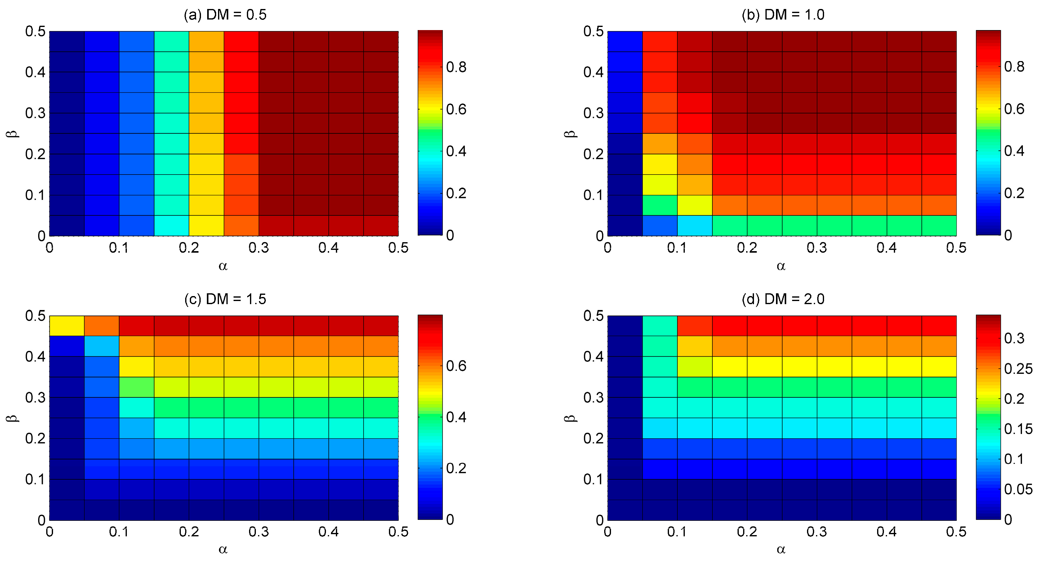
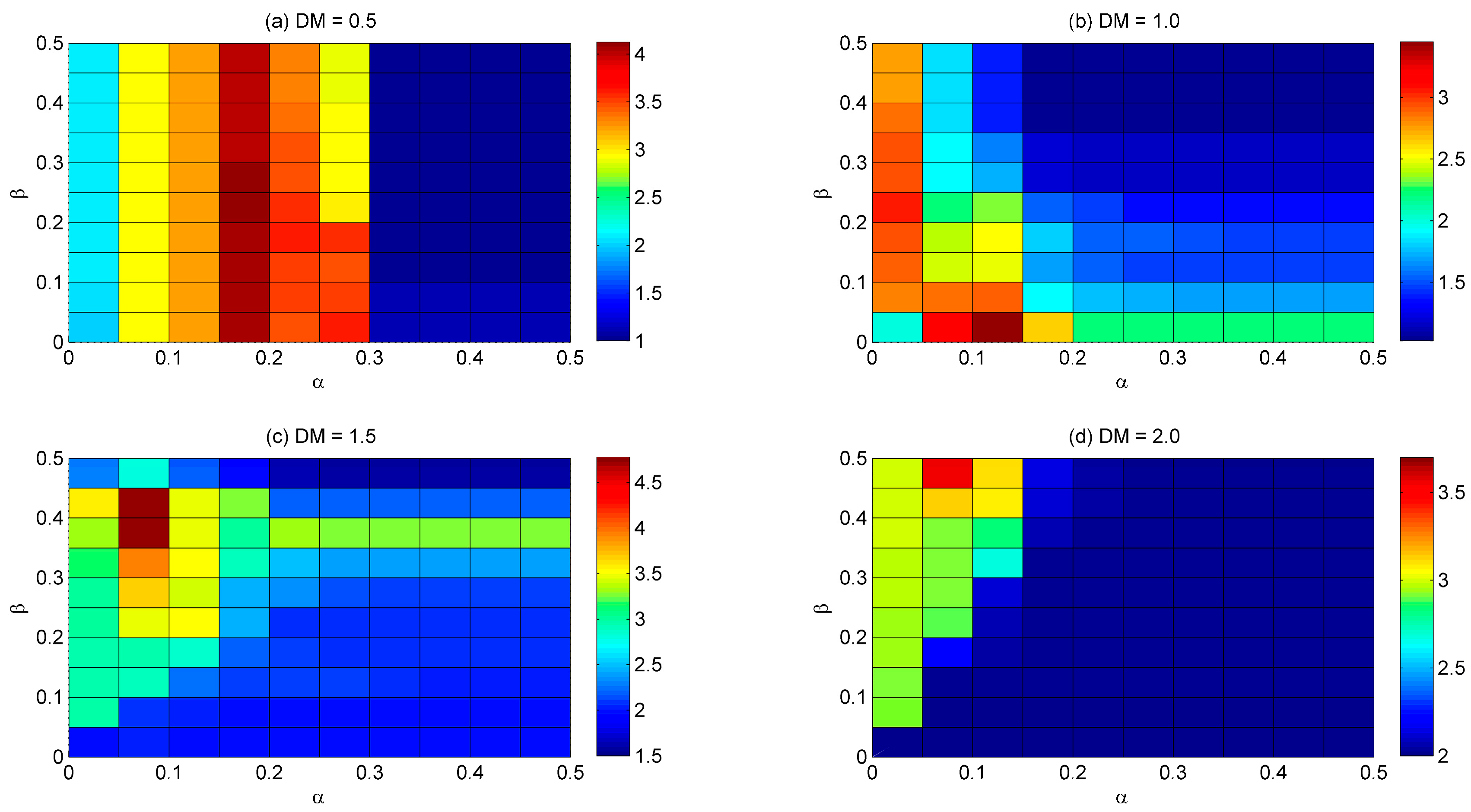
For a pipe-based attack, Figure 2 and Figure 3 display the evolution process of system reliability and failure propagation time with different DM conditions. The Z axis describes system reliability, whereas the X and Y axes describe tolerant parameters α and β, respectively. The gradual color change from dark blue to red indicates the system reliability changing from weak to strong.
It can be observed that the system has a stronger potential ability to absorb and withstand local failures with increases in α and β. The evaluation of the system reliability and failure propagation time shows the same change pattern.
It can be seen that the influence of the highest capacity (α) and lowest capacity (β) on the system reliability and failure propagation time are different. To be specific, when DM < 1.0, the system reliability and failure propagation time change in the direction of α. Conversely, the influence that β has on the system reliability and failure propagation time becomes stronger when DM ≥ 1.0, exceeding the influence that α has, thus becoming the dominant factor that decides the evolution of system reliability and failure propagation time.
3.3. System Reliability Evolution with Fixed DM
Valves are a crucial factor in evaluating the reliability of a system under cascading failures. Unfortunately, valve data on the existing case were not provided. The valve rate VR is used in this section. In the previous section, we discuss the impact of DM with a fixed VR. In this section, DM is fixed as 1.0 and the influence of VR is then analyzed.
In the simulation process, values of VR are set at 10% to 100% with an interval of 10%. WDN only has a few valves at VR = 10%, while at VR = 100%, each pipe is placed with two valves at its initial and terminal nodes, respectively. Valves are located randomly with different VR. It is assumed that the minimum pressure for each node is 35 m. To obtain system reliability, α changes from 0 to 0.5 with an interval of 0.05 with each VR, and each VR scenario is simulated 30 times. Hence the total simulation time for each VR scenario is 330. The average values are then calculated.
It can be seen in Figure 2 that system reliability can achieve a stable value, i.e., system reliability would not change with the tolerance parameter variation. The stable value of system reliability and VR are picked. The results are drawn in Figure 4.
The relationship of system reliability, failure propagation time, and VR presents a flattened S curve relationship. System reliability increases with increasing VR. After a few valves are located, the WDN is able to resist cascading failures. However, the resistance of the cascading effect is not obvious with these small amounts of valves. System reliability grows rapidly when VR runs over 20%, and the growth rate slows down after VR is greater than 80%.
The S curve relationship can be divided into three stages.
The first stage is the initial phase of system reliability. In this stage, the VR changes slowly. It is difficult to isolate cascading failures after the pipe is broken. Secondary failures in WDN spread rapidly. System reliability remains unchanged when the VR is between 10% and 20%. It can be seen that the VR has no significant effect on system reliability under cascading failures when the VR is lower than 20%.
The second stage is the accelerated phase of system reliability. With the VR rising to more than 20%, an effective isolation appears in WDN to prevent cascading failures propagation. The auxiliary line of system reliability increasing with the growth of VR is drawn. It can be seen that system reliability is lower than the auxiliary line when the VR is less than 60%. System reliability and the auxiliary line are basically flat when the VR is near 65%. When the VR is larger than 70%, system reliability exceeds the auxiliary line. The growth rate of system reliability increases with the increase of the VR.
The third stage is the mature phase of system reliability. The growth of system reliability slows down when the VR is larger than 80%. The 100% valve placement can be the most effective against cascading failures. However, when the VR exceeds a certain percentage, the added valves do not lead to a sustained and stable growth of the WDN resisting cascading failures. It is obvious that the system reliability growth rate decelerates when the VR increases over 80%. Actually, it is costly and unrealistic to set valves at both ends of every pipe. For the case WDN, a VR up to 80% can effectively resist cascading failures.
For the analysis of failure propagation time, WDN fails rapidly when the VR is low, because there is no isolation and effective protection methods taken. When the valves are located in WDN, the isolation makes the failure propagation time longer. WDN shows a step-by-step failure process. The failure propagation time reaches its peak value when the VR is equal to 50%. The condition of VR > 50% can reduce the failure propagation time effectively, and then it shows a decreasing trend.
3.4. Critical Pipes
Considering the analysis in Section 3.3, there are two turning points at the VR values of 20% and 80%, and they bring significant changes in WDN system reliability. In this section, VR = 20% and VR = 80% are taken to analyze the critical pipes in WDN. The purpose is to find the critical pipes that will cause the system reliability to be reduced greatly after the valves are located. Set α increases from 0 to 0.5 with an interval of 0.05, i.e., a total of 11 scenarios. Each pipe in the WDN is taken as the initial failure. For each pipe, the VR scenario is simulated 30 times with 11 α scenarios. Calculate the average value of system reliability in the 330 simulations experiencing cascading failures of each pipe. The valley points of system reliability both in VR = 20% and VR = 80% are the WDN critical pipes.
The result of the system reliability at VR = 20% and VR = 80% after the initial failure of a certain pipe is shown in Figure 5. When the VR is equal to 20%, system reliability fluctuates from 0.046 to 0.208. System reliability of Pipe 5 and Pipe 33 is higher than the others. There exists many lower reliability values, such as Pipes 4, 8, 13, and 22. When the VR is equal to 80%, system reliability is higher than that with the VR equal to 20%. There are many higher reliability values, such as Pipes 6, 10, 19, 24, 28, 39, and 40. After Pipe 22 fails, the WDN shows the lowest system reliability, and the second lowest value corresponding to Pipe 8.
The critical pipes are the ones whose system reliability are valley points both with VR = 20% and VR = 80%. For example, Pipe 4’s system reliability (4.64%) is the second lowest value as VR = 20%, while its system reliability (82.00%) ranks eleventh by sorting from big to small as VR = 80%. Hence, Pipe 4 is not able to be used as the critical pipe of WDN. In contrast, Pipe 8 and Pipe 22 reduce WDN system reliability dramatically both with VR = 20% and VR = 80%. Therefore, Pipe 8 and Pipe 22 are identified as the critical pipes in the case WDN.
3.5. Valve Adjustment
The failure of critical pipes has a serious impact on the reliability of the WDN. To protect the WDN, valves can be added to the critical pipes which have been recognized in Section 3.4. For further analysis of whether the identification and adjustment scheme is effective, the improvements are measured in this section.
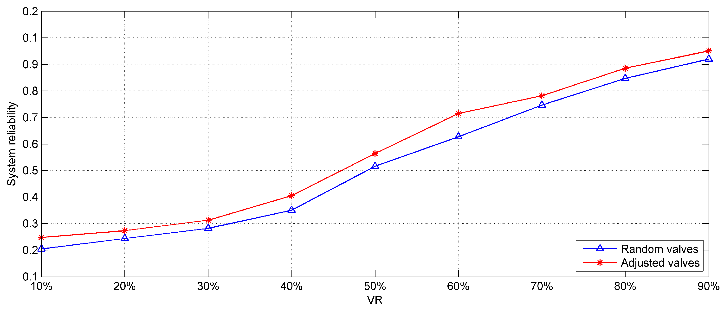
In the valve adjustment scheme, valves are located at both ends of Pipe 8 and Pipe 22. Other valves are located randomly. In the random located scheme, all the valves are located randomly. The random failure of a pipe is simulated in the WDN. If the pipe break triggers cascading failures, then we continue to simulate cascading failures until the WDN reaches stable. Calculate the system reliability after cascading failures stop. By comparing the system reliability of the two schemes, the improvement is tested. Each VR scenario is simulated 550 times, and the average value is calculated.
The results are shown in Figure 6. System reliability of the two schemes both increase with the growth of the VR. It can be found that the system reliability has improved significantly from VR = 10% to VR = 90%. The maximum improvement reaches 8.76% (VR = 60%).
There are 40 pipes in the case WDN. The N valve rule isolation indicates that one pipe has two valves at opposite nodes. In this case, up to 80 valves can be located in WDN. According to the method in this paper, fixing four valve locations, i.e., 5% of the 80 valve locations, can enhance the WDN system reliability effectively.
4. Discussion
In this paper, a simulation-based method for evaluating the system reliability of WDNs experiencing cascading failures is presented. The pipe-based intentional attack scenario is simulated. The proposed procedure considers how the attack pattern, the balance of water supply and demand, the valve locations, and pressure constraints impact the process that leads to failure propagation. Using one specific WDN derived from real systems, the effects of such factors on system reliability for several combinations of demand multiplier DM, tolerant parameters corresponding to highest capacity (i.e., α) and lowest capacity (i.e., β), and valve ratio VR are showcased.
The dynamic process of system reliability and failure propagation time is first evaluated. The proposed method contributes to the literature by combining the network topology and water service characteristics with attack patterns that cause cascading failures in WDNs. Unlike topology-based methods, the valve isolation, the redistribution of water hydraulics, and updates to the network structure are analyzed. In addition, complex network studies pay close attention to the highest capacity. However, simulations in this paper illustrate that the lowest capacity is also a significant factor in WDN. Given cascading failures, the WDN system reliability and failure propagation time depend not only on the highest capacity and network topology but also on the lowest capacity and variations in water supply and demand. The results revealed that the influence of the lowest capacity increases when the WDN is short of supply, exceeding the highest capacity as the dominant factor that decides the evolution of system reliability and failure propagation time.
The influence of valve location with WDN resisting cascade failures is then discussed. Valve location is an important way for a WDN to resist cascading failures. According to the N valve rule, each pipe has at most two valves on both ends of the pipe. However, in reality, it is difficult to achieve this valve arrangement due to its high cost. In order to better analyze the influence of VR on WDN resisting cascade failures, the paper simulates the system reliability evolution with VR from 10% to 100%. It can be found that the VR and system reliability presents a flattened S curve relationship. There are two turning points in VR. The resistance is not obvious with a small number of valves. The resistance is a less marked increase with the growth of VR after VR exceeds a certain number.
In addition, a WDN quickly fails when a small amount of valves is located. After a certain number of valves are located in a WDN, the step-by-step cascading propagation is displayed and the failure propagation time becomes longer. A large number of valves can effectively stop the spread of cascading failure. Hence, the failure propagation time decreases steadily.
Besides, the critical pipes which can result in WDN system reliability reducing dramatically are identified. The turning points of VR are taken into consideration. The critical pipes are defined as the pipes in which the system reliability is lower than the others in VR turning points.
Furthermore, the effectiveness of the identified critical pipes is measured. Valves are located on both ends of the critical pipe. The improvement of the valve adjustment scheme and random located scheme is compared. The results show that the valve adjustment scheme (i.e., fixing 5% of the 80 valve locations) is able to improve the WDN system reliability and resist cascading failures effectively.
Nonetheless, the paper only considers one case for simulation. There are still remaining challenges for future research. With the proposed method, part of the future work will focus on network redundancy and repair time assessments as emergency strategies to enhance system reliability. Also, an unsteady flow can occur which might generate pipe breaks not far from the failure event. The unsteady flow in WDN needs to be considered in the simulation. The failure propagation time in the paper describes a discrete cascading failure process. The system reliability should be changed taking into account the integral along the time of both the actual and required demand, where the discrete failure propagation time refines to continuous time intervals. The reliability evaluation of a WDN should consider the guarantee of water quantity and water quality. The model established in this paper does not consider water quality. It is necessary to incorporate the safety of water quality into the model.
Acknowledgments
This work was funded by the National Natural Science Foundation of China under Grant No. 71501008, the Fundamental Funds for Humanities and Social Sciences of Beijing Jiaotong University (No. 2015jbwj014), and the Fundamental Funds of Beijing Jiaotong University (No. 2015RC002). The authors also gratefully acknowledge the helpful comments and suggestions of the reviewers, which have improved the model.
Author Contributions
Q.S. designed and conceptualized the study and prepared the first draft of the paper; Q.S. and K.S. preformed the experiments; Q.S., Y.L., and K.S. analyzed the data; Y.L. contributed the analysis tools; Y.T. performed the data inventory. J.L. prepared the figures. All authors contributed to the writing of the paper.
Conflicts of Interest
The authors declare no conflict of interest. The founding sponsors had no role in the design of the study; in the collection, analyses, or interpretation of data; in the writing of the manuscript, and in the decision to publish the results.
References
- Gheisi, A.; Forsyth, M.; Naser, G. Water Distribution Systems Reliability: A Review of Research Literature. J. Water Resour. Plan. Manag. 2016, 142, 04016047. [Google Scholar] [CrossRef]
- Yazdani, A.; Otoo, R.A.; Jeffrey, P. Resilience enhancing expansion strategies for water distribution systems: A network theory approach. Environ. Model. Softw. 2011, 26, 1574–1582. [Google Scholar] [CrossRef]
- Yang, S.L.; Hsu, N.S.; Loule, P.W.F.; Yeh, W.W.G. Water distribution network reliability: Connectivity analysis. J. Infrastruct. Syst. 1996, 2, 54–64. [Google Scholar] [CrossRef]
- Adachi, T. Impact of Cascading Failures on Performance Assessment of Civil Infrastructure Systems. Ph.D. Thesis, Georgia Institute of Technology, Atlanta, GA, USA, May 2007. Available online: https://smartech.gatech.edu/handle/1853/14543 (accessed on 8 June 2017).
- Wang, J.W.; Rong, L.L. Robustness of the western United States power grid under edge attack strategies due to cascading failures. Saf. Sci. 2011, 49, 807–812. [Google Scholar] [CrossRef]
- Zhang, Y.; Yang, N. Research on robustness of R&D network under cascading propagation of risk with gray attack information. Reliab. Eng. Syst. Saf. 2013, 117, 1–8. [Google Scholar] [CrossRef]
- Wang, W.X.; Chen, G. Universal robustness characteristic of weighted networks against cascading failure. Phys. Rev. E 2008, 77, 026101. [Google Scholar] [CrossRef] [PubMed]
- Motter, A.E.; Lai, Y.C. Cascade-based attacks on complex networks. Phys. Rev. E 2002, 66, 065102. [Google Scholar] [CrossRef] [PubMed]
- Li, S.; Li, L.; Yang, Y.; Luo, Q. Revealing the process of edge-based-attack cascading failures. Nonlinear Dyn. 2012, 69, 837–845. [Google Scholar] [CrossRef]
- Albert, R.; Jeong, H.; Barabasi, A.L. Error and attack tolerance of complex networks. Nature 2000, 409, 378–382. [Google Scholar] [CrossRef] [PubMed]
- Kennedy, D. Science, terrorism, and natural disasters. Science 2002, 295, 405. [Google Scholar] [CrossRef] [PubMed]
- Su, Y.C.; Mays, L.W.; Duan, N.; Lansey, K.E. Reliability-Based Optimization Model for Water Distribution Systems. J. Hydraul. Eng. 1987, 113, 1539–1556. [Google Scholar] [CrossRef]
- Tanyimboh, T.T.; Tabesh, M.; Burrows, R. Appraisal of Source Head Methods for Calculating Reliability of Water Distribution Networks. J. Water Resour. Plan. Manag. 2001, 127, 206–213. [Google Scholar] [CrossRef]
- Ostfeld, A.; Kogan, D.; Shamir, U. Reliability simulation of water distribution systems—Single and multiquality. Urban Water 2002, 4, 53–61. [Google Scholar] [CrossRef]
- Gheisi, A.; Naser, G. Water distribution system reliability under simultaneous multicomponent failure scenario. J. Am. Water Works. Assoc. 2014, 106, E319–E327. [Google Scholar] [CrossRef]
- Berardi, L.; Ugarelli, R.; Røstum, J.; Giustolisi, O. Assessing mechanical vulnerability in water distribution networks under multiple failures. Water Resour. Res. 2014, 50, 2586–2599. [Google Scholar] [CrossRef]
- Gheisi, A.; Naser, G. Multistate Reliability of Water-Distribution Systems: Comparison of Surrogate Measures. J. Water Resour. Plan. Manag. 2015, 141, 04015018. [Google Scholar] [CrossRef]
- Laucelli, D.; Giustolisi, O. Vulnerability Assessment of Water Distribution Networks under Seismic Actions. J. Water Resour. Plan. Manag. 2015, 141, 04014082. [Google Scholar] [CrossRef]
- Yazdani, A.; Jeffrey, P. Complex network analysis of water distribution systems. Chaos 2011, 21, 016111. [Google Scholar] [CrossRef] [PubMed]
- Hawick, K.A. Water Distribution Network Robustness and Fragmentation using Graph Metrics. In Proceedings of the International Conference on Water Resource Management, Gaborone, Botswana, Africa, 3–5 September 2012; pp. 1–8. [Google Scholar] [CrossRef]
- Yazdani, A.; Jeffrey, P. A complex network approach to robustness and vulnerability of spatially organized water distribution networks. arXiv Preprint 2010, 1–18. [Google Scholar]
- Sitzenfrei, R.; Mair, M.; Möderl, M.; Rauch, W. Cascade vulnerability for risk analysis of water infrastructure. Water Sci. Technol. 2011, 64, 1885–1891. [Google Scholar] [CrossRef] [PubMed]
- Hines, P.; Cotilla-Sanchez, E.; Blumsack, S. Do topological models provide good information about vulnerability in electric power networks? Chaos 2010, 20, 033122. [Google Scholar] [CrossRef] [PubMed]
- Ouyang, M. review on modeling and simulation of interdependent critical infrastructure systems. Reliab. Eng. Syst. Saf. 2014, 121, 43–60. [Google Scholar] [CrossRef]
- Ouyang, M. Comparisons of purely topological model, betweenness based model and direct current powerflow model to analyze power grid vulnerability. Chaos 2013, 23, 023114. [Google Scholar] [CrossRef] [PubMed]
- Torres, J.M.; Duenas-Osorio, L.; Li, Q.; Yazdani, A. Exploring Topological Effects on Water Distribution System Performance Using Graph Theory and Statistical Models. J. Water Resour. Plan. Manag. 2016, 143, 04016068. [Google Scholar] [CrossRef]
- Dueñas-Osorio, L.; Vemuru, S.M. Cascading failures in complex infrastructure systems. Struct. Saf. 2009, 31, 157–167. [Google Scholar] [CrossRef]
- Wang, J.; Zhang, C.; Huang, Y.; Xin, C. Attack robustness of cascading model with node weight. Nonlinear Dyn. 2014, 78, 37–48. [Google Scholar] [CrossRef]
- Hernandez-Fajardo, I.; Dueñas-Osorio, L. Probabilistic study of cascading failures in complex interdependent lifeline systems. Reliab. Eng. Syst. Saf. 2013, 111, 260–272. [Google Scholar] [CrossRef]
- Shuang, Q.; Zhang, M.; Yuan, Y. Node vulnerability of water distribution networks under cascading failures. Reliab. Eng. Syst. Saf. 2014, 124, 132–141. [Google Scholar] [CrossRef]
- Mays, L.W. Reliability analysis of water distribution systems. Reliab. Anal. Water Distrib. Syst. 1989, 120, 472–532. [Google Scholar]
- Ostfeld, A. Reliability analysis of regional water distribution systems. Urban Water 2001, 3, 253–260. [Google Scholar] [CrossRef]
- Duan, N.; Mays, L.W.; Lansey, K.E. Optimal reliability-based design of pumping and distribution systems. J. Hydraul. Eng. 1990, 116, 249–269. [Google Scholar] [CrossRef]
- Shinstine, D.S.; Ahmed, I.; Lansey, K.E. Reliability/availability analysis of municipal water distribution networks: Case studies. J. Water Resour. Plan. Manag. 2002, 128, 140–151. [Google Scholar] [CrossRef]
- Bondy, J.A.; Murty, U.S.R. Graph Theory with Applications, 1st ed.; The Macmillan Press: New York, NY, USA, 1976; p. 171. ISBN 0-444-19451-7. [Google Scholar]
- Chai, C.L.; Liu, X.; Zhang, W.J.; Baber, Z. Application of social network theory to prioritizing Oil & Gas industries protection in a networked critical infrastructure system. J. Loss Prev. Process Ind. 2011, 24, 688–694. [Google Scholar] [CrossRef]
- Laucelli, D.; Berardi, L.; Giustolisi, O. Assessing climate change and asset deterioration impacts on water distribution networks: Demand driven or pressure-driven network modeling? Environ. Model. Softw. 2012, 37, 206–216. [Google Scholar] [CrossRef]
- Zhuang, B.; Lansey, K.; Kang, D. Reliability/availability analysis of water distribution systems considering adaptive pump operation. In Proceedings of the World Environmental and Water Resources Congress, Palm Springs, CA, USA, 22–26 May 2011; pp. 224–233. [Google Scholar] [CrossRef]
- Wagner, J.M.; Shamir, U.; Marks, D.H. Water distribution reliability-simulation methods. J. Water Resour. Plan. Manag. 1988, 114, 276–294. [Google Scholar] [CrossRef]
- Giustolisi, O.; Walski, T.M. Demand components in water distribution network analysis. J. Water Resour. Plan. Manag. 2012, 138, 356–367. [Google Scholar] [CrossRef]
- Rossman, L.A. EPANET 2 User’s Manual, 1st ed.; National Risk Management Research Laboratory, Environmental Protection Agency: Cincinnati, OH, USA, 2000. [Google Scholar]
- Giustolisi, O.; Savic, D. Identification of segments and optimal isolation valve system design in water distribution networks. Urban Water J. 2010, 7, 1–15. [Google Scholar] [CrossRef]
- Jun, H.; Loganathan, G.V. Valve-Controlled Segments in Water Distribution Systems. J. Water Resour. Plan. Manag. 2007, 133, 145–155. [Google Scholar] [CrossRef]
- Walski, T.M. Water distribution valve topology for reliability analysis. Reliab. Eng. Syst. Saf. 1993, 42, 21–27. [Google Scholar] [CrossRef]
- Zhuang, B.; Lansey, K.; Kang, D. Resilience/availability analysis of municipal water distribution system incorporating adaptive pump operation. J. Hydraul. Eng. 2013, 139, 527–537. [Google Scholar] [CrossRef]
- Cormen, T.H.; Stein, C.; Rivest, R.L.; Leiserson, C.E. Introduction to Algorithms, 2nd ed.; The MIT Press and McGraw-Hill Book Company: New York, NY, USA, 2001; ISBN 0-262-03293-7. [Google Scholar]
- Darvini, G.; Salandin, P.; Deppo, L.D. Coping with uncertainty in the reliability evaluation of water distribution systems. In Proceedings of the 10th Annual Water Distribution Systems Analysis Conference, Skukuza, South Africa, 17–20 August 2008; pp. 483–498. [Google Scholar] [CrossRef]
- Islam, M.S.; Sadiq, R.; Rodriguez, M.; Najjaran, H.; Hoorfar, M. Reliability assessment for water supply systems under uncertainties. J. Water Resour. Plan. Manag. 2014, 140, 468–479. [Google Scholar] [CrossRef]
Figure 1.
The layout for the water distribution network (WDN).
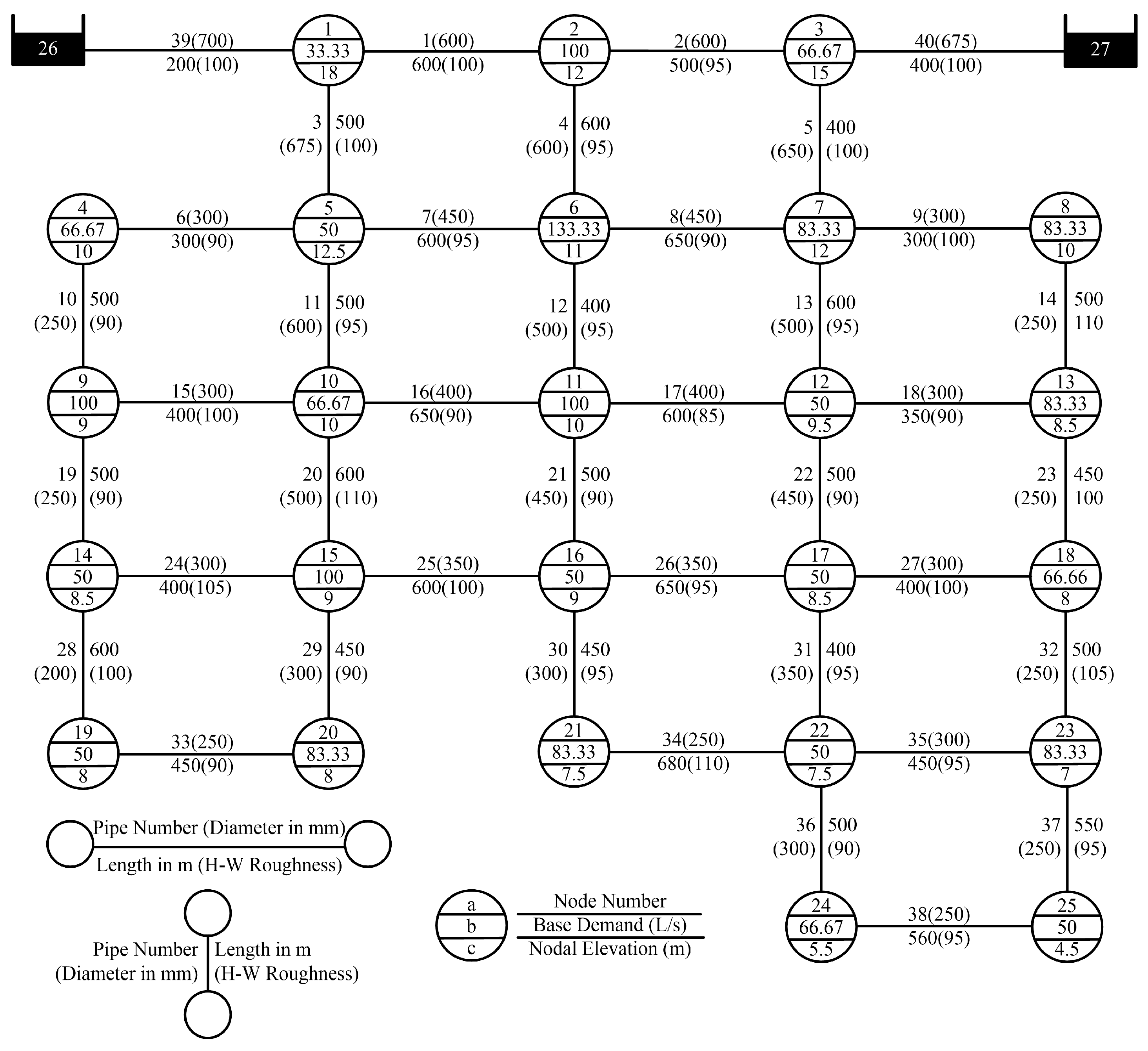
Figure 2.
The evolution process of system reliability with different DM conditions: (a) DM = 0.5; (b) DM = 1.0; (c) DM = 1.5; (d) DM = 2.0.
Figure 2.
The evolution process of system reliability with different DM conditions: (a) DM = 0.5; (b) DM = 1.0; (c) DM = 1.5; (d) DM = 2.0.

Figure 3.
The evolution process of failure propagation time with different DM conditions: (a) DM = 0.5; (b) DM = 1.0; (c) DM = 1.5; (d) DM = 2.0.
Figure 3.
The evolution process of failure propagation time with different DM conditions: (a) DM = 0.5; (b) DM = 1.0; (c) DM = 1.5; (d) DM = 2.0.

Figure 4.
The relationship of system reliability, failure propagation time, and valve ratio (VR).
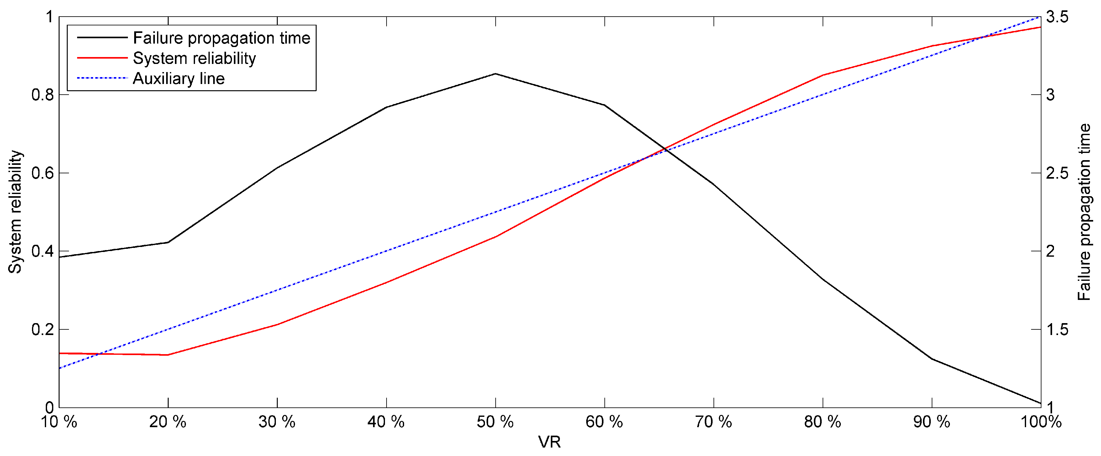
Figure 5.
System reliability at VR = 20% and VR = 80%.
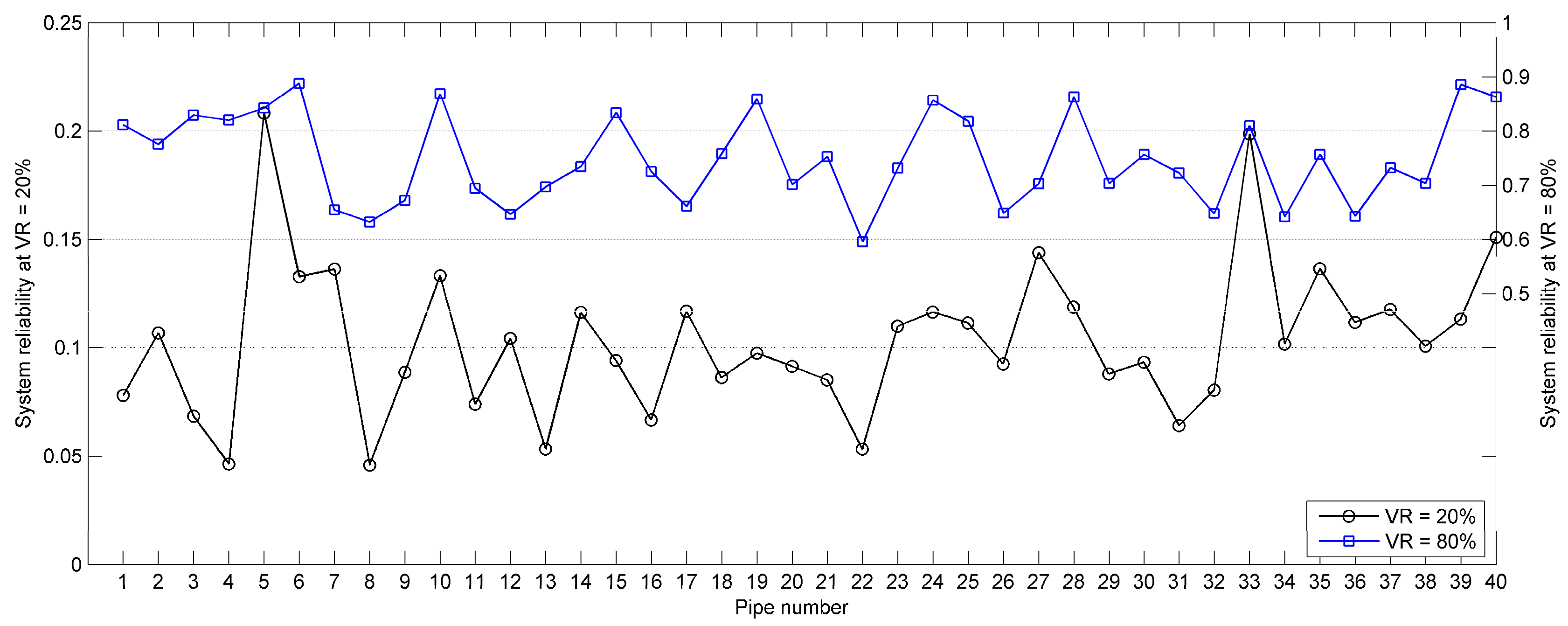
Figure 6.
System reliability of the valve adjustment scheme and the random located scheme.

Table 1.
Nodal pressures in the initial balance state.
| Node Number | 1 | 2 | 3 | 4 | 5 | 6 | 7 | 8 | 9 |
| Pressure (m) | 86.91 | 84.30 | 84.35 | 78.66 | 82.92 | 82.14 | 82.16 | 77.09 | 76.14 |
| Node Number | 10 | 11 | 12 | 13 | 14 | 15 | 16 | 17 | 18 |
| Pressure (m) | 79.30 | 78.88 | 77.89 | 74.54 | 74.91 | 76.20 | 75.88 | 74.24 | 71.53 |
| Node Number | 19 | 20 | 21 | 22 | 23 | 24 | 25 | - | - |
| Pressure (m) | 69.65 | 70.27 | 69.91 | 68.82 | 66.85 | 64.70 | 64.36 | - | - |
Table 2.
The maximum value of system reliability (MVSR) results for varied demand multiplier (DM) values.
Table 2.
The maximum value of system reliability (MVSR) results for varied demand multiplier (DM) values.
| DM | MVSR | DM | MVSR | Reduction | DM | MVSR | Reduction | DM | MVSR | Reduction |
|---|---|---|---|---|---|---|---|---|---|---|
| 0.5 | 0.975 | 1.0 | 0.9725 | 0.26% | 1.5 | 0.7989 | 17.85% | 2.0 | 0.3391 | 57.55% |
© 2017 by the authors. Licensee MDPI, Basel, Switzerland. This article is an open access article distributed under the terms and conditions of the Creative Commons Attribution (CC BY) license (http://creativecommons.org/licenses/by/4.0/).
Share and Cite
MDPI and ACS Style
Shuang, Q.; Liu, Y.; Tang, Y.; Liu, J.; Shuang, K. System Reliability Evaluation in Water Distribution Networks with the Impact of Valves Experiencing Cascading Failures. Water 2017, 9, 413. https://doi.org/10.3390/w9060413
AMA Style
Shuang Q, Liu Y, Tang Y, Liu J, Shuang K. System Reliability Evaluation in Water Distribution Networks with the Impact of Valves Experiencing Cascading Failures. Water. 2017; 9(6):413. https://doi.org/10.3390/w9060413
Chicago/Turabian StyleShuang, Qing, Yisheng Liu, Yongzhong Tang, Jing Liu, and Kai Shuang. 2017. "System Reliability Evaluation in Water Distribution Networks with the Impact of Valves Experiencing Cascading Failures" Water 9, no. 6: 413. https://doi.org/10.3390/w9060413
Note that from the first issue of 2016, this journal uses article numbers instead of page numbers. See further details here.