
Gridded Snow Water Equivalent Reconstruction for Utah Using Forest Inventory and Analysis Tree-Ring Data


1
Department of Plants, Soils and Climate and the Utah Climate Center, Utah State University, 4820 Old Main Hill, Logan, UT 84322, USA
2
USDA Forest Service, Forest Inventory and Analysis, Rocky Mountain Research Station, 507 25th Street, Ogden, UT 84401, USA
*
Author to whom correspondence should be addressed.
Water 2017, 9(6), 403; https://doi.org/10.3390/w9060403
Submission received: 10 March 2017
/
Revised: 23 May 2017
/
Accepted: 30 May 2017
/
Published: 6 June 2017
Abstract
:Snowpack observations in the Intermountain West are sparse and short, making them difficult for use in depicting past variability and extremes. This study presents a reconstruction of April 1 snow water equivalent (SWE) for the period of 1850–1989 using increment cores collected by the U.S. Forest Service, Interior West Forest Inventory and Analysis program (FIA). In the state of Utah, SWE was reconstructed for 38 snow course locations using a combination of standardized tree-ring indices derived from both FIA increment cores and publicly available tree-ring chronologies. These individual reconstructions were then interpolated to a 4-km grid using an objective analysis with elevation correction to create an SWE product. The results showed a significant correlation with observed SWE as well as good correspondence to regional tree-ring-based drought reconstructions. Diagnostic analysis showed statewide coherent climate variability on inter-annual and inter-decadal time-scales, with added geographical details that would not be possible using courser pre-instrumental proxy datasets. This SWE reconstruction provides water resource managers and forecasters with better spatial resolution to examine past variability in snowpack, which will be important as future hydroclimatic variability is amplified by climate change.
1. Introduction
Water supplies in the U.S. Intermountain West will be affected by a decrease in snowpack compounded by an amplified fluctuation of snowpack variability [1,2,3,4,5]; this tendency may be particularly pronounced in the topographically diverse state of Utah [6]. To further complicate water issues, Utah has a rapidly growing population that is currently straining water resources. Utah’s climate can be characterized as warm to hot-humid continental climate type, with hot, dry summers and cold winters [7]. Precipitation amounts are typically highest in the spring and lowest in the summer, but winter storms bring copious amounts of snow to the mountains. This leads to the development of heavy snowpack that is a critical form of water storage for the state. During the winter months (October thru March), nearly 70% of mountain precipitation arrives as snow [8]. This accumulation of snowpack peaks near April 1 and then melts gradually over the summer, and is an important source of runoff. However, the snow water equivalent (SWE) of accumulated snowpack varies widely by location within the state. While 1000 mm is typical, in northern Utah snowpack measurement stations sometimes exceed 1500 mm, while in the southern portion of the state 500 mm is usual. Recent research has suggested that Utah snowpack is declining [6], and understanding the climate controls on past snowpack will help water managers plan for the future. Furthermore, understanding the temporal and spatial variability of SWE prior to instrumentation will improve water resource management and forecasting.
While numerous studies have indicated the possibility for both decreased snowpack and increased variability in snowpack accumulation across the west, subsequent changes in the timing and distribution of peak and annual runoff are also likely [9,10]. However, a relatively short period of instrumental record (starting approximately in 1930) in the Intermountain West limits our understanding of snowpack variability. Fortunately, in the western U.S. tree-ring data have been used to create a broad range of climate reconstructions including precipitation (e.g., [11,12]), temperature (e.g., [13]), and streamflow (e.g., [14,15,16]), as well as snowpack for parts of the Rocky Mountains [17,18,19,20], and could be employed for high resolution reconstructions of SWE.
Tree-ring-based climate reconstructions rely on intensive sampling of trees that have been carefully selected from site(s) and/or species thought to record a climatic variable of interest and can be replicated [21]. Subsequently, statistical reconstruction models rely on the presence and length of tree-ring chronologies across a given region. There have been important efforts to create gridded datasets with broad spatial coverage using tree-ring chronologies, notably for temperature and precipitation [22], as well as the Palmer Drought Severity Index (PDSI) [23]. These gridded products have proven to be useful for the analysis of long-term climate variability at regional to continental scales. These datasets become more limited, however, when it comes to analyzing watershed-scale variability within complex terrain such as that found in the Intermountain West (see Figure 1). The production of multiple tree-ring chronologies that would enable fine-scale and broad-coverage reconstructions is desirable. However, chronologies are extremely time-consuming and cost-prohibitive to develop, thus alternative data are also highly desirable.
As has been noted in several studies [16,24,25] there are large gaps in the spatial coverage of publicly available tree-ring chronologies (International Tree-Ring Data Bank, ITRDB). Some of the largest gaps are over central and northern Utah, and southeastern Idaho. Because of the previously mentioned difficulties posed by collecting and building tree-ring chronologies everywhere, DeRose et al. [24] explored the possibility of using increment cores collected by the U.S. Forest Service, Forest Inventory and Analysis (FIA) program as potential proxies for climate reconstructions, and as an alternative means to address the paucity of data in the region. The FIA program monitors and characterizes the nation’s forest resources through the use of a comparatively high-density sampling grid (see Section 2.2) and a sampling strategy that resulted in the collection of a large number of increment cores on a geographically unbiased grid (~5 km spacing) throughout the Intermountain West, including Utah.
The feasibility of species-specific subsets of the FIA tree-ring dataset in depicting climate variability has been previously demonstrated in DeRose et al. [24]. In general, increment cores from low elevation species (Psuedotsuga menziesii and Pinus edulis) were significantly correlated with water-year (Aug-Jul) precipitation, and in particular over mountainous areas, and were moderately negatively correlated with temperature. Given that accumulated SWE and water-year precipitation are closely correlated [8], it is reasonable to assume that the FIA tree-ring data will serve as a proxy for SWE as well. Therefore, in this paper we develop a reconstruction of April 1 SWE using the FIA tree-ring data combined with any available tree-ring chronologies in the region. We evaluate the reconstructed grid of SWE based on statistical tests, and by comparison with other gridded products. Climate diagnostics are performed to demonstrate the utility and application of the gridded SWE data to water resources management.
2. Materials and Methods
2.1. Observational and Climate Data
SWE observations from a total of 38 snow courses were obtained from the U.S. Department of Agriculture’s Natural Resources Conservation Service (NRCS, http://www.wcc.nrcs.usda.gov/snow/, Figure 1). Locations were selected that had a common period of record covering 1930–1989. All courses selected had no more than 10% of the record without observations (i.e., only six or fewer missing values). Many of these courses have longer records, but some FIA collections in Utah were conducted as early as 1989, so a later date for the calibration period could not be used. Details of snow course data and their collection can be found at http://www.wcc.nrcs.usda.gov/factpub/sect_4a.html. The NRCS automated Snow Telemetry (SNOTEL) data were not used here due to the insufficient temporal coverage (no data prior to the early 1980s). We also note that, while SNOTEL observations are considered by many as the “truth” regarding snowpack conditions, these data have drawbacks; known biases include those caused by wind, aspect, and canopy (e.g., [26]). These drawbacks extend to snow course measurement as well; the standardized sampling device used for NRCS snow course measurements has been shown to overestimate SWE by about 10% [27].
As part of the validation of our reconstructions, we used the North American Drought Atlas (NADA) [23] to compare spatial variability between reconstructed SWE and drought. We also used an unsmoothed tripole index for the Inter-decadal Pacific Oscillation (IPO) created from Hadley Center sea ice and sea surface temperature data [28] to test for any relationship between IPO and Utah SWE.
2.2. Tree-Ring Data
At each FIA sampling plot, a suite of measurements are made periodically in order to characterize forest attributes and change over time [29,30]. As part of the Interior West FIA program, increment cores were collected from a subset of trees on each plot to establish plot ages and periodic growth rates. These trees represent the dominant species on the plot in terms of size and forest type. Because increment cores were sampled to represent dominant forest types, many tree species are represented in the FIA tree-ring data set. For this study, we used cores collected from P. menziesii and P. edulis, all of which grow at relatively low elevations and exhibit ring-width variability known to reasonably reflect moisture availability. These species are potentially susceptible to drought and have been shown to be appropriate for use as climate proxies (e.g., [11,31]). The FIA increment cores were subsequently measured and cross-dated, and each time-series was then detrended. In an attempt to remove the effects of stand dynamics and biological growth patterns, we used a cubic smoothing spline with a frequency response of 0.5 at a wavelength of 2/3 times the tree-ring series length [32]. In our region of interest (36.5–43.5 N, 114.5–107.5 W), there was a total of 967 FIA samples. Some of these samples did not provide sufficient temporal coverage (i.e., young trees) for our intended reconstruction period of 1850–1990, and thus were excluded; after our selection process, which included temporal coverage and species, the final number of FIA plots included in our study as potential predictors was 110.
The FIA tree-ring ring-width indices were supplemented by (a) 31 P. menziesii and P. edulis chronologies available from the ITRDB and (b) 31 additional tree-ring chronologies developed by the Wasatch Dendroclimatology Research group, WADR [33]. These chronologies were developed for the species P. menziesii, P. edulis, P. ponderosa, Juniperus scopulorum, and J. osteosperma, and have been used in reconstructions of streamflow for the Logan River [25] and Weber River [16], and of Great Salt Lake (GSL) water level [34]. The WADR chronologies in particular provided added sample depth for northern Utah, where both FIA samples and ITRDB samples were sparse (Figure 1).
2.3. Reconstruction Method
The FIA tree-ring data were evaluated for temporal consistency of their relationship to 1 April SWE using correlations. Low correlations indicated possible instability, and high correlations were necessary to be included in the models. For each snow course, the tree-ring data with the highest correlations (both concurrent with observations and lagged one year) were then used in a multiple linear regression model, of the form:
built in a stepwise fashion by adding predictors one at a time, ranging from one predictor to a maximum of 12, objectively determined to maintain model parsimony. We set no spatial control on potential model predictors such that any snow course site could be modeled by any combination of tree-ring data. The predictive potential of each model was tested using the predictive error sum of squares (PRESS; [35]), a leave-one-out validation method taking the form:
where n = number of observations, is the ith observation, and is the predicted value of when was excluded from the regression. For each snow course, the regression model with the smallest PRESS and thus the highest predictive skill was selected as the final model.
As metrics for model performance, we report variance explained (R2), as well as adjusted R2, calculated as:
where n = sample size and k = number of predictors. This test penalized the addition of predictors and thus reduced the inflation of R2 due simply to additional regression parameters, and thereby provided a stricter test [36]. We also used a cross-validated R2 based on the PRESS statistic:
In the case of poor predictive models, can take negative values if PRESS is greater than total sum of squares (TSS), that is if model predictions are worse than using the observational data.
2.4. Gridded Interpolation
After regression modeling, the reconstructed SWE for all snow courses were interpolated to a regular rectangular grid. Such a grid extended the usefulness of data by enabling the integration of SWE estimates over space, and resulted in estimates of total snowpack water content over a region. Previous, gridded SWE datasets have been created with ground observations [37] and satellite measurements [38], but are less common than other gridded climate variables such as temperature and precipitation and have limited temporal coverage (post-1978).
In this study, the combined SWE reconstructions were interpolated to a regular grid using Cressman objective analysis [39,40] to 4-km resolution, similar to the grid spacing used by the PRISM dataset [41]. Cressman analysis used an iterative process of considering station data within successively smaller radii of influence to determine the interpolated value. We used four radii of influence: 3°, 2°, 1°, and ½° for our grids. A data mask was applied to any grid points with an elevation below 1800 m (~6000 ft.), where there is generally not snowpack accumulation. Because Cressman analysis did not account for orography in the gridding process, we adjusted the grid point values using:
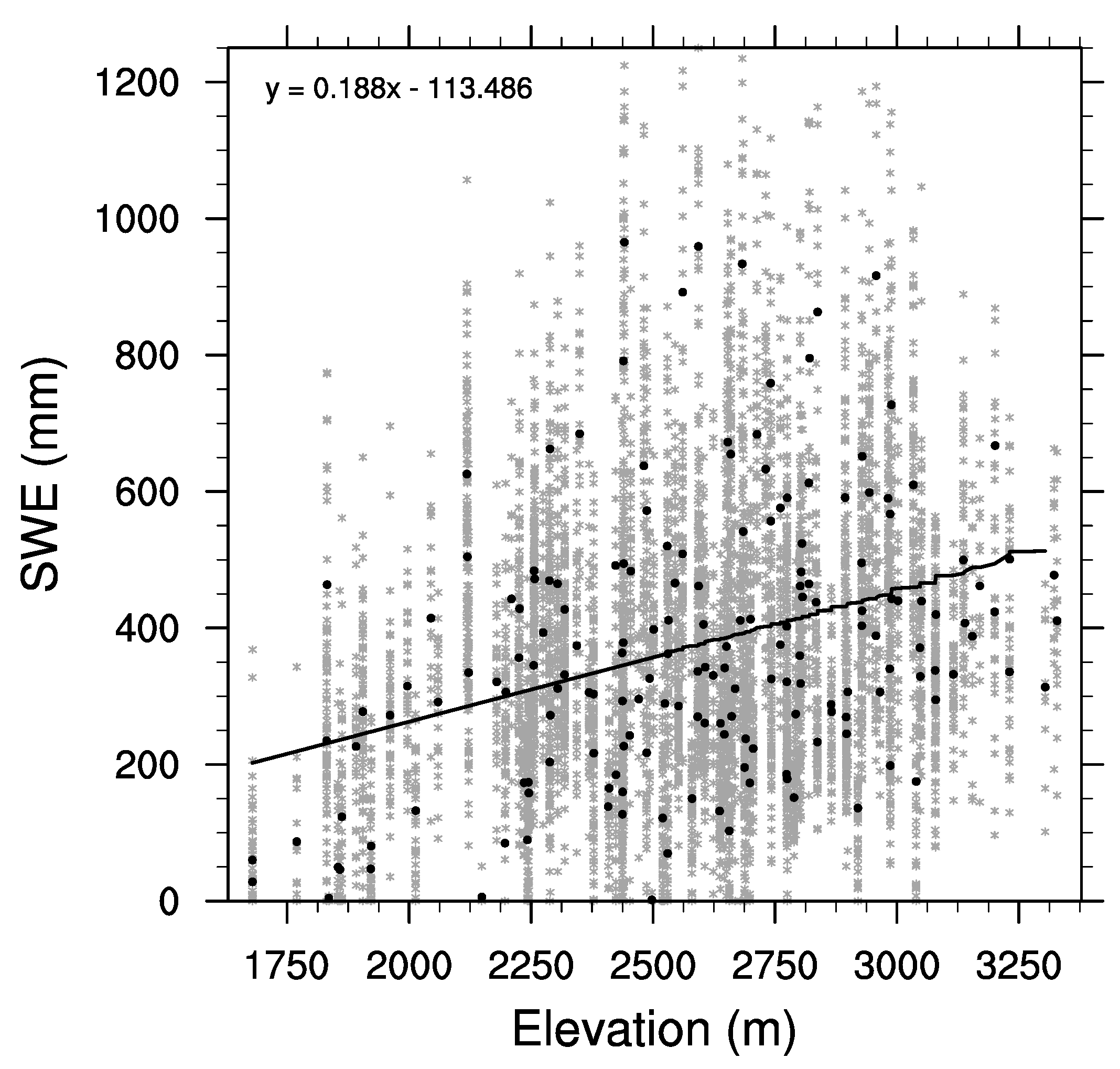
where = elevation of grid point and = average elevation of snow courses used in the reconstruction. This took into account the relationship between SWE observations and elevation in the data set (Figure 2). Cressman analysis also assumed that the data being interpolated have spatial and temporal stationarity; however, this assumption might not hold true with our data. To address the potential for spatial non-stationarity, we added dummy observations in our region of interest filled with zeroes, essentially zero-padding the data. This was accomplished by adding 250 locations, which were assigned using a random number generator, provided that the locations were at least 75 km from any snow course location, and yielded a density of dummy locations that was similar to the density and distribution of the snow courses stations. The zero-padding approach was intended only to minimize extrapolation problems at the edges of the domain, and was not necessarily an assumption that the point was actually snow-free (Figure 3).
2.5. Climate Diagnostics
To test the added value of including the FIA data in these reconstructions, we applied our methodology to two sets of data: (1) all tree-ring data, which included the FIA plots, and (2) by including only the ITRDB and WADR tree-ring chronologies. We tested for model improvement in the all tree-ring data model by conducting a modified F-test to compare models with a potentially different number of parameters. We further investigated the spatial and temporal dynamics of the gridded SWE reconstruction by the application of an empirical orthogonal function (EOF) analysis, which indicated the major modes of variability in space and time in a particular dataset. Specifically, we correlated the first and second principal components (PC) derived from the SWE reconstruction and the NADA, and we performed a spectral decompostion of both PCs. Finally, we used the IPO index, low-pass filtered at four years to eliminate high-frequency noise, and performed a lagged correlation analysis on the first and second PCs. We chose IPO because it characterizes pan-Pacific tropical sea surface temperature anomalies [42] that represent both inter-annual events (i.e., El Niño/Southern Oscillation, ENSO) as well as the decadal to multi-decadal variability inherent in such teleconnections as the Pacific Decadal Oscillation or the Quasi-Decadal Oscillation.
3. Results
3.1. Calibration and Model Validation
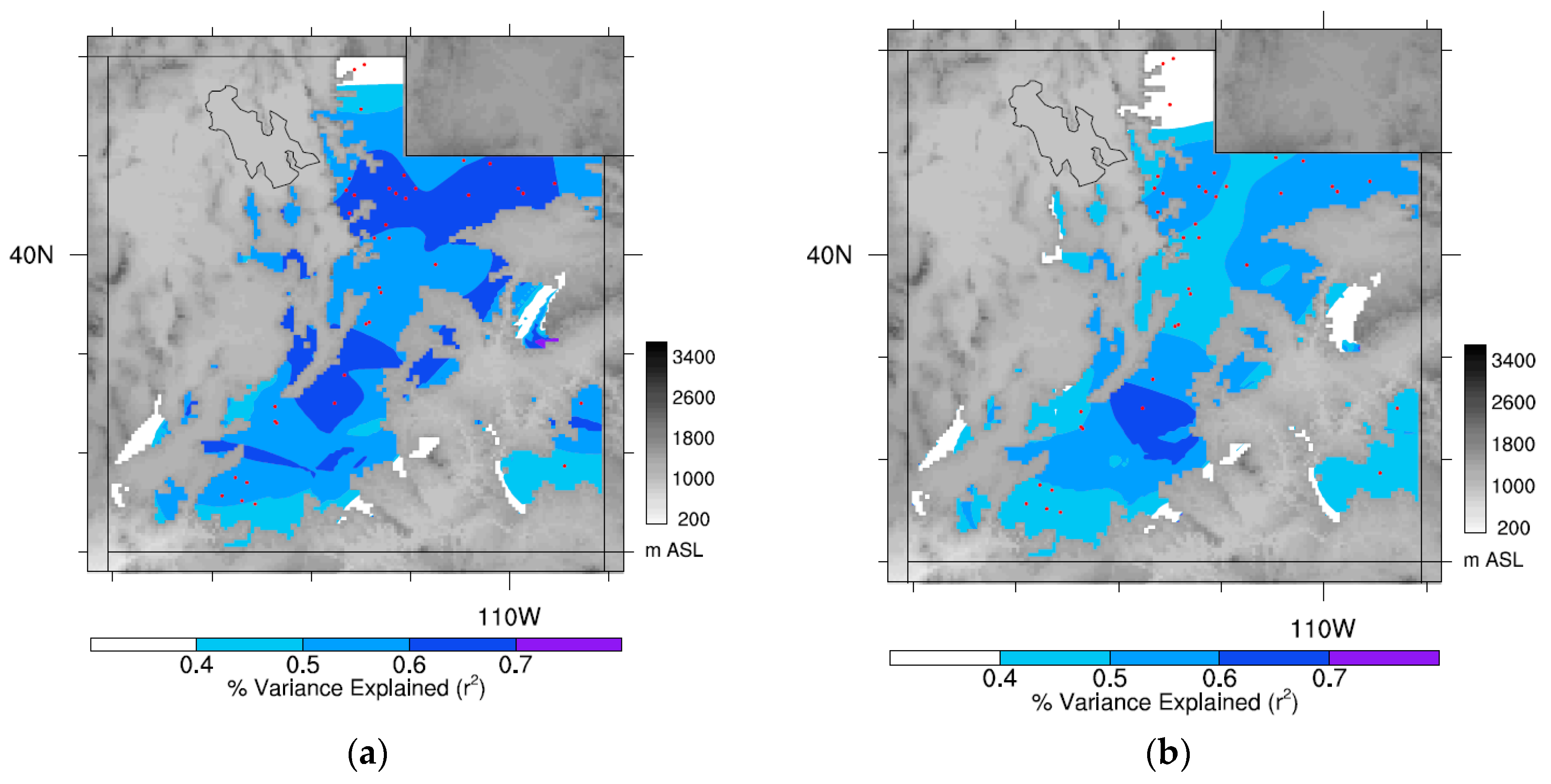
Reconstructed SWE model skill () varied across the 38 snow coreses used in the state from as low as 0.25 to as high as 0.71, but averaged 0.49 when all tree-ring data were used. Model verification also varied across the state, ranged from 0.23 to 0.67, and averaged 0.46, and ranged from 0.17 to 0.59, and averaged 0.36 (Table S1). Limiting the tree-ring data to ITRDB and WADR data reduced the range of skill to 0.18–0.62, and averaged 0.43, when compared to the full tree-ring data set. Model verification on the reduced tree-ring data set resulted in that ranged from 0.15 to 0.57, and averaged 0.4, and ranged from 0.09 to 0.49, and averaged 0.34 (Table S2). Fully 60% of the snow courses had significantly higher skill when FIA data were included, than with tree-ring chronologies alone (Table S1). Therefore, overall the full tree-ring data set produced the gridded reconstruction with the highest skill, where all but five of the snow courses yielded an R2 of at least 0.4, and over half exceeded 0.5. Depicted spatially, the gridded results for the individual reconstructions indicated the relationships (R2) between the reconstructed and observed grids. Almost the entire grid scored above 0.4 despite the predictor data set (Figure 4). However, the use of the FIA tree-ring data enhanced the spatial representation of model skill when compared to the reduced data set (Figure 4a versus Figure 4b), where the model skill for almost the entire state exceeded 0.5.
3.2. EOF Analysis and Climate Diagnostics
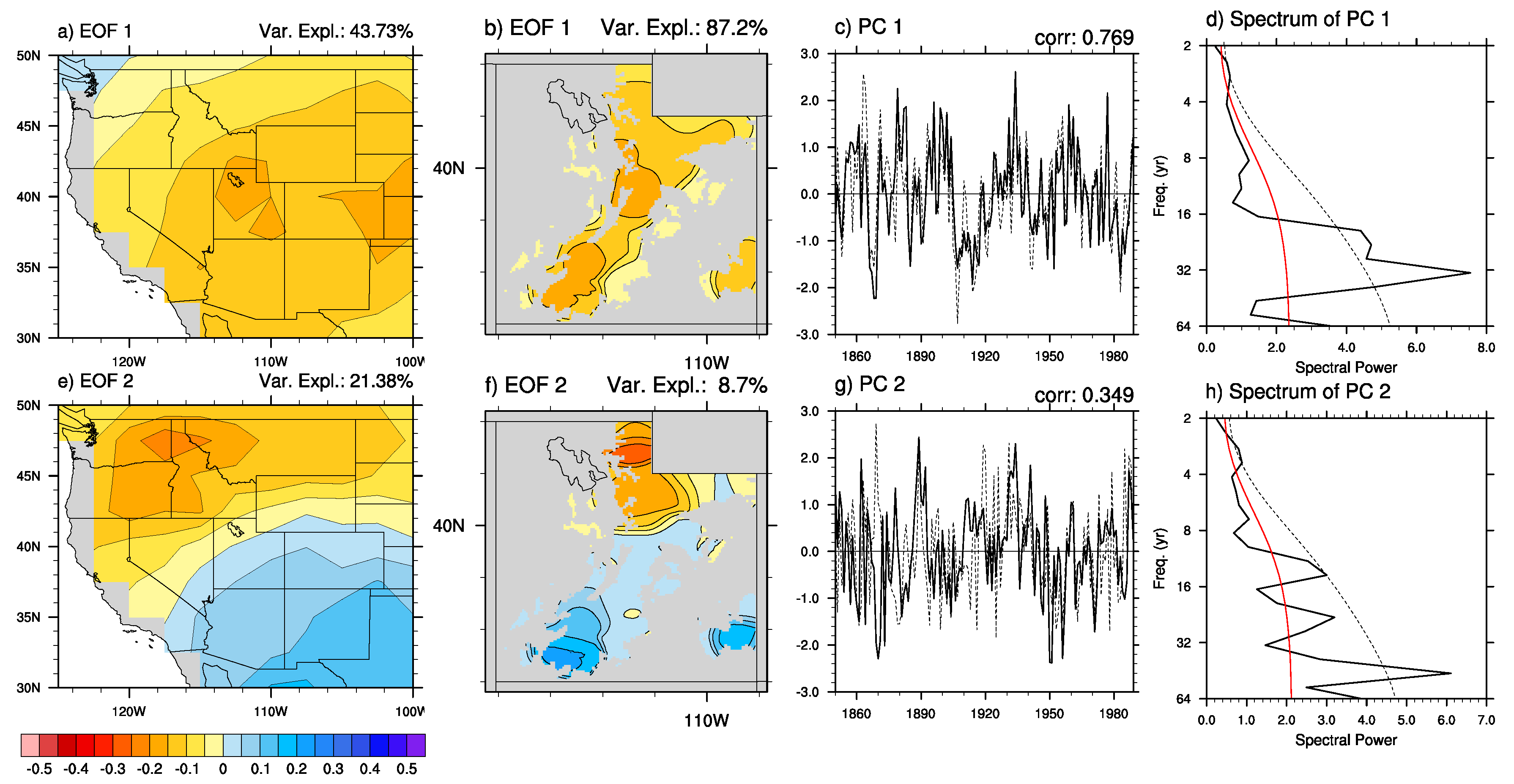
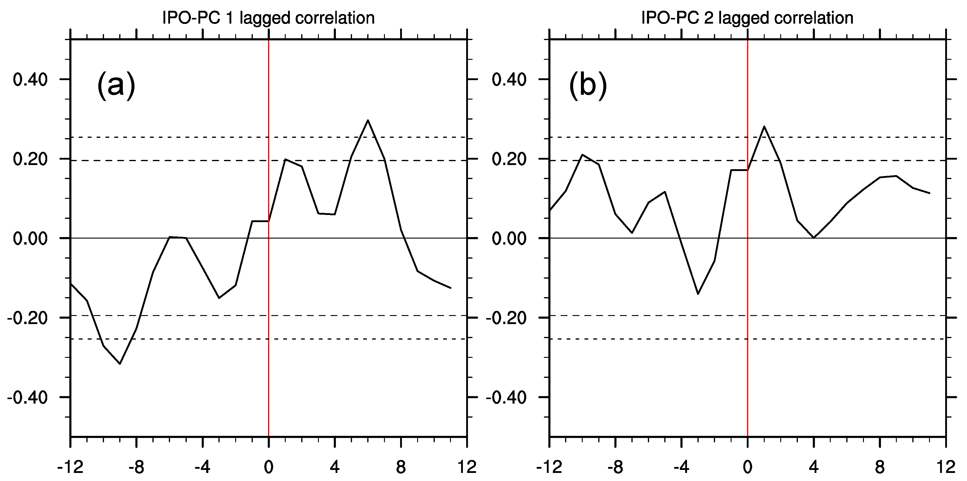
EOF 1 indicated statewide coherent variability in the FIA tree-ring-based SWE reconstruction, and was by far the largest mode of variability (~87%). EOF 2 showed a northwest-southeast dipole, indicated by a much weaker mode (~9%). In comparison, the first leading mode for both the FIA-based reconstruction and the NADA explained 87.2% and 43.7% of the variability, respectively, and were depicted similarly over space (Figure 5a,b). Likewise, the second leading mode for FIA and the NADA explained an additional 8.7% and 21.4% of the variability, respectively, and had reasonably similar spatial representation (Figure 5e,f). While the first two modes of variability in the FIA-based reconstruction explained over 95% of the total variance, the first two modes of NADA explained ~67%. Furthermore, both principle component (1 & 2) time-series for the SWE reconstruction compared to NADA were highly significantly correlated (p < 0.01, Figure 5c,g). Significant periodicity at 2–4 years and ~16–40 years was apparent in PC1 of the SWE reconstruction (Figure 5d). For PC2 there was significant periodicity at 4, 12 and ~50 year frequencies (Figure 5h). Finally, lagged correlation between PC1 the low pass-filtered IPO was significant (p < 0.01) at a lag of 6 years, whereas the relationship for PC2 was significant at a lag of 1 year (Figure 6).
4. Discussion
The SWE reconstruction indicated particularly good skill in the southern and central Wasatch and central Uinta Mountains, which are crucial areas for snowpack water storage as they feed into the largest and most important tributaries in the region, the Great Basin and the Colorado Basin. The reconstruction skill is consistent with, but shows improvement over, the results in DeRose et al. [24] where water-year precipitation was correlated with FIA tree-ring data and showed the strongest relationships in mountainous regions. In comparison, the gridded reconstruction created without the FIA tree-ring data showed reduced variance explained throughout the entire state. One important similarity between both reconstruction grids is the failure to adequately explain a few snow courses in the extreme northern portion of the state. Increasing predictive skill in this region should be the subject of future inquiry. It should be noted that while the variance explained by these regression models is lower than that reported in water-year or streamflow reconstructions (which can produce R2 values as high as ~0.7), April 1 is an arbitrarily selected time to measure SWE that is nonetheless accepted as a standard for water resource management because in many years this date provides a reasonable estimate of peak snowpack. Ideally, peak SWE is a better estimate of water availability, and therefore potential tree growth, but such data are not available prior to the SNOTEL era (early 1980s).
As in any regression modeling context, the amount of variance explained decreases from R2 to due to the differing number of parameters. Similarly, our chosen metric of validation, , will be necessarily lower than statistics that describe model fit. The relationship among fit statistics resulted in some interesting patterns that bear further scrutiny. In a number of models, the addition of FIA predictors resulted in better R2 (e.g., King’s Cabin-Upper, Silver Lake-Brighton, Panguitch Lake), but the improvement was not statistically significant. In contrast, there were a number of sites where the addition of FIA data did not noticeably change the model fit (e.g., Mosby Mountain, Garden City Summit, Mammoth-Cottonwood). In most of these situations the stations were located at very high elevations (greater than approximately 2900 m), suggesting that our modeling approach, which was composed of almost entirely low-elevation P. menziesii and P. edulis as predictors in both datasets, might be enhanced by incorporating other less-conventional species [43]. Although these species have been shown to be moisture-sensitive in this region, and therefore some tree growth would be associated with moisture that arrived other than from snowpack, there was ~30–50% variance left unexplained within our SWE reconstructions. At least part of this may be due to the indirect linkage between tree growth and previous winter snowpack. Regardless, given the close relationship between accumulated snowpack and water-year precipitation in the region, we are confident in the validity of our reconstruction. Finally, in some situations the no-FIA model actually produced higher skill (e.g., Fish Lake), which was a result of applying our stepwise linear models independently. Although, it is not unreasonable to expect tree-ring chronologies, in the absence of more local FIA data, to produce high skill models.
While our analyses suggested that the gridded SWE data in Utah were broadly consistent with drought variability at the regional scale, it should be noted that some of the predictors (i.e., ITRDB chronologies) were likely used in the creation of both our reconstruction and the NADA, and so some correspondence should be expected. It is also worth noting that the NADA was calibrated for the June, July, August season, while April 1 SWE is the result of winter precipitation, so we suggest that the similarity of the PCs between reconstructions is more than simply a statistical artifact, but rather reflects the effect of broad-scale climatic drivers on regional-scale hydroclimatology (i.e., accumulated snowpack is the primary source of moisture for the region, and therefore will have a strong influence on drought indices).
Comparison of Spatial Variability
The periodicity seen in PC1 is consistent with the prominent quasi-decadal variability recorded by the PDSI in Utah [44] and Great Salt Lake levels [45]. These studies proposed that this unique climate variability is caused by a type of teleconnection excited during the transitional phases of the Pacific quasi-decadal oscillation (QDO), rather than the extreme warm/cold phases that appeared in the central tropical Pacific in previous research on Great Salt Lake levels [46,47]. This connection was also found with the IPO, which occurs on a ~30 year frequency; this finding, along with the PDSI analysis of Herweijer et al. [48], lends support to the multidecadal variability found in PC1 of reconstructed SWE. Additionally, although PC1 had a much stronger effect (i.e., explained more variance) than PC2, when both occur simultaneously such as in 1934 (Figure 5c–g), the reduction in SWE can be severe. The year 1934 was one of the strongest regional drought years in Utah, often used as the drought year-of-record in water management, which coincided with the Dust Bowl era. This result indicates that ENSO forcing can be modulated by the larger-scale and stronger effects linked with PC1 or the Pacific QDO’s transition phases, as was the case proposed for the Dust Bowl [42], and record floods in northern Utah [49] and the Missouri River Basin [50]. Indeed, the significant correlation of PC1 to IP at a lag of six years is consistent with the transition-phase teleconnection presented by Wang et al. [47].
Variability in the second mode was consistent with ENSO-driven variability in terms of spatial patterns (i.e., the north/south dipole), the relatively weak loading, and the lower percentage of variance explained. This second mode corroborates previous observations that Utah lies along the fulcrum of the regional-scale, north-south ENSO dipole [44,51,52,53]. The correlation between PC2 and the IPO at a lag of one year was consistent with ENSO forcing. These modes of variability were strikingly consistent with the first two modes found in the EOF analysis of NADA [23], in which EOF1 exhibited domain-wide coherent behavior with a regional center over Utah. By comparison, EOF2 of the continental-scale PDSI depicted the ENSO dipole with the wet/dry division cutting across Utah. However, the NADA provides only a coarse representation of the location of the dipole fulcrum; EOF2 of gridded SWE depicted much more clearly the spatial representation of this fulcrum, which bisected the northern Wasatch Mountains from the central Utah plateau region, and the Uinta Mountains from the Uinta Basin. The dipole indicated that in some years the response to ENSO within Utah can be opposed in extreme northern or southern domains, and that little correspondence to ENSO can be expected for central portions of Utah.
5. Conclusions
The gridded, high resolution (4 km), SWE reconstruction represents a useful proxy of past mountain snowpack at the watershed level. Observational data in the Intermountain West are sparse and have limited temporal coverage at primarily low elevations (except the more recent SNOTEL), and therefore are difficult for use in depicting past climate extremes. Our SWE reconstruction for Utah more than doubled the temporal coverage available from instrumental records (i.e., snow courses). Because the understanding of historical controls on snowpack variability provides insight into snowpack conditions, any extended record of SWE like the one presented here can help improve our understanding of hydroclimatic variability, and specifically on water availability and climate change impacts in the region. The results of the analyses here help indicate which areas of the state are likely to respond to relative changes in climatic forcing (e.g., ENSO versus IPO-driven) in the future, which can influence water availability forecasting. In an era of decreasing snowpack, understanding the watershed-level detail of past snowpack will be important for water managers and water management. Furthermore, understanding the potential repercussions of the simultaneous occurrence of the primary and secondary modes of variability in the region will help water managers anticipate and plan for extreme droughts (e.g., 1934) or extreme pluvials (e.g., early 1980s), in particular, given that the primary modes of SWE variability statewide is predominantly driven by decadal to multi-decadal climate forcing. The FIA tree-ring data and the reconstructed SWE grid data are provided to the public at http://cliserv.jql.usu.edu/FIAdata/.
Supplementary Materials
The following are available online at www.mdpi.com/2073-4441/9/6/403/s1, Table S1: Summary statistics for snow course reconstructions using all tree-ring data. Table S2: Summary statistics for snow course reconstructions using only ITRDB and WADR tree-ring data.
Acknowledgments
Funding for this study came from the U.S. Dept. of the Interior’s WaterSMART Initiative R13AC80039, and the Utah State University Agricultural Experiment Station (9005). Special thanks to the Wasatch Dendroclimatology Research group and the Utah State Dendrochronology Laboratory for preparation of the FIA increment cores. This paper was prepared in part by an employee of the US Forest Service as part of official duties and is therefore in the public domain.
Author Contributions
D.B., S.-Y.S.W. and R.J.D. conceived and designed the experiments; D.B. performed the experiments; D.B. analyzed the data; R.J.D. contributed tree-ring data; D.B., S.-Y.S.W., and R.J.D. wrote the paper.
Conflicts of Interest
The authors declare no conflict of interest.
References
- Nash, L.L.; Gleick, P.H. Sensitivity of streamflow in the Colorado Basin to climatic changes. J. Hydrol. 1991, 125, 221–241. [Google Scholar] [CrossRef]
- Barnett, T.P.; Adam, J.C.; Lettenmaier, D.P. Potential impacts of a warming climate on water availability in snow-dominated regions. Nature 2005, 438, 303–309. [Google Scholar] [CrossRef] [PubMed]
- Wise, E.K. Hydroclimatology of the US Intermountain West. Prog. Phys. Geogr. 2012, 36, 1–22. [Google Scholar] [CrossRef]
- Woodbury, M.; Balso, M.; Yates, D.; Kaatz, L. Joint Front Range Climate Change Vulnerability Study; Water Research Foundation Rep: Denver, CO, USA, 2012; 148p. [Google Scholar]
- Mote, P.W. Climate-Driven Variability and Trends in Mountain Snowpack in Western North America. J. Clim. 2006, 19, 6209–6220. [Google Scholar] [CrossRef]
- Gillies, R.R.; Wang, S.-Y.; Booth, M.R. Observational and synoptic analyses of the winter precipitation regime change over Utah. J. Clim. 2012, 25, 4679–4698. [Google Scholar] [CrossRef]
- Mock, C.J. Climatic controls and spatial variations of precipitation in the western United States. J. Clim. 1996, 9, 1111–1125. [Google Scholar] [CrossRef]
- Serreze, M.C.; Clark, M.P.; Armstrong, R.L.; McGinnis, D.A.; Pulwarty, R.S. Characteristics of the western United States snowpack from snowpack telemetry (SNOTEL) data. Water Resour. Res. 1999, 35, 2145–2160. [Google Scholar] [CrossRef]
- Stewart, T.S.; Cayan, D.R.; Dettinger, M.D. Changes toward Earlier Streamflow Timing across Western North America. J. Clim. 2005, 18, 1136–1155. [Google Scholar] [CrossRef]
- Clow, D.W. Changes in the timing of snowmelt and streamflow in Colorado: A response to recent warming. J. Clim. 2009, 23, 2293–2306. [Google Scholar] [CrossRef]
- Knight, T.A.; Meko, D.M.; Baisan, C.H. A bimillennial-length tree-ring reconstruction of precipitation for the Tavaputs Plateau, northeastern Utah. Quat. Res. 2010, 73, 107–117. [Google Scholar] [CrossRef]
- Gray, S.T.; Fastie, C.L.; Jackson, S.T.; Betancourt, J.L. Tree-ring-based reconstructions of precipitation in the Bighorn Basin, Wyoming, since 1260 A.D. J. Clim. 2004, 17, 3855–3865. [Google Scholar] [CrossRef]
- Briffa, K.R.; Jones, P.D.; Schweingruber, F.H. Tree-ring density reconstruction of summer temperature patterns across western North America since 1600. J. Clim. 1992, 5, 735–754. [Google Scholar] [CrossRef]
- Carson, E.C.; Munroe, J.S. Tree-ring based streamflow reconstruction for Ashley Creek, northeastern Utah: Implications for palaeohydrology of the southern Uinta Mountains. Holocene 2005, 15, 602–611. [Google Scholar] [CrossRef]
- Woodhouse, C.A.; Lukas, J.J. Drought, Tree Rings and Water Resource Management in Colorado. Can. Water Resour. J. Rev. Can. Ressour. Hydr. 2006, 31, 297–310. [Google Scholar] [CrossRef]
- Bekker, M.F.; Justin DeRose, R.; Buckley, B.M.; Kjelgren, R.K.; Gill, N.S. A 576-Year Weber River Streamflow Reconstruction from Tree Rings for Water Resource Risk Assessment in the Wasatch Front, Utah. JAWRA J. Am. Water Resour. Assoc. 2014, 50, 1338–1348. [Google Scholar] [CrossRef]
- Woodhouse, C.A. A 431-yr reconstruction of western Colorado snowpack from tree tings. J. Clim. 2003, 16, 1551–1561. [Google Scholar] [CrossRef]
- Timilsena, J.; Piechota, T. Regionalization and reconstruction of snow water equivalent in the upper Colorado River basin. J. Hydrol. 2008, 352, 94–106. [Google Scholar] [CrossRef]
- Pederson, G.T.; Gray, S.T.; Woodhouse, C.A.; Betancourt, J.L.; Fagre, D.B.; Littell, J.S.; Watson, E.; Luckman, B.H.; Graumlich, L.J. The Unusual Nature of Recent Snowpack Declines in the North American Cordillera. Science 2011, 333, 332–335. [Google Scholar] [CrossRef] [PubMed]
- Anderson, S.; Moser, C.L.; Tootle, G.A.; Grissino-Mayer, H.D.; Timilsena, J.; Piechota, T. Snowpack Reconstructions Incorporating Climate In the Upper Green River Basin (Wyoming). Tree-Ring Res. 2012, 68, 105–114. [Google Scholar] [CrossRef]
- Fritts, H.C. Tree Rings and Climate; Academic Press: Cambridge, MA, USA, 1976. [Google Scholar]
- Fritts, H.C. Reconstructing Large-Scale Climatic Patterns from Tree-Ring Data: Diagnostic Analysis; University of Arizona Press: Tuscon, AZ, USA, 1991. [Google Scholar]
- Cook, E.R.; Krusic, P.J. The North American Drought Atlas. Lamont-Doherty Earth Observatory and the National Science Foundation. Available online: https://www.ncdc.noaa.gov/data-access/paleoclimatology-data/datasets/tree-ring/north-american-drought-variability (accessed on 10 June 2016).
- DeRose, R.J.; Wang, S.-Y.; Shaw, J.D. Feasibility of high-density climate reconstruction based on Forest Inventory and Analysis (FIA) collected tree-ring data. J. Hydrometeorol. 2013, 14, 375–381. [Google Scholar] [CrossRef]
- Allen, E.B.; Rittenour, T.M.; DeRose, R.J.; Bekker, M.F.; Kjelgren, R.; Buckley, B.M. A tree-ring based reconstruction of Logan River streamflow, northern Utah. Water Resour. Res. 2013, 49, 8579–8588. [Google Scholar] [CrossRef]
- Meyer, J.D.D.; Jin, J.; Wang, S.-Y. Systematic patterns of the inconsistency between snow water equivalent and accumulated precipitation as reported by the snowpack telemetry network. J. Hydrometeorol. 2012, 13, 1970–1976. [Google Scholar] [CrossRef]
- Farnes, P.E.; Peterson, N.R.; Goodison, B.E.; Richards, R.P. Metrication of manual snow sampling equipment. In Proceedings of the 50th Annual Western Snow Conference, Reno, NV, USA, 20–23 April 1982. [Google Scholar]
- Henley, B.J.; Gergis, J.; Karoly, D.J.; Power, S.; Kennedy, J.; Folland, C.K. A Tripole Index for the Interdecadal Pacific Oscillation. Clim. Dyn. 2015, 45, 3077–3090. [Google Scholar] [CrossRef]
- McRoberts, R.E.; Bechtold, W.A.; Patterson, P.L.; Scott, C.T.; Reams, G.A. The enhanced Forest Inventory and Analysis Program of the USDA Forest Service: Historical perspective and announcement of statistical documentation. J. For. 2005, 103, 304–308. [Google Scholar]
- Smith, W.B. Forest inventory and analysis: A national inventory and monitoring program. Environ. Pollut. 2002, 116, s233–s242. [Google Scholar] [CrossRef]
- Watson, E.; Luckman, B.H. The dendroclimatic signal in Douglas-fir and ponderosa pine tree-ring chronologies from the southern Canadian Cordillera. Can. J. For. Res. 2002, 32, 1858–1874. [Google Scholar] [CrossRef]
- Cook, E.R. A Time Series Analysis Approach to Tree Ring Standardization (Dendrochronology, Forestry, Dendroclimatology, Autoregressive Process); The University of Arizona: Tucson, AZ, USA, 1985. [Google Scholar]
- Rittenour, T.M.; Kjelgren, R.; Bekker, M.F.; DeRose, R.J.; Buckley, B.M.; Wang, S.-Y.; Hipps, L.; Gillies, R.; Allen, E.B.; Sriladda, C.; et al. The Wasatch Dendroclimatology Research (WADR) group: Multi-disciplinary investigations into the paleoclimatology of Northern Utah as recorded in tree-ring series. In Proceedings of the USU Spring Runoff Conference, Utah State University, Logan, UT, USA, 3–4 April 2012. [Google Scholar]
- DeRose, R.J.; Wang, S.-Y.; Buckley, B.M.; Bekker, M.F. Tree-ring reconstruction of the level of Great Salt Lake, USA. Holocene 2014, 24, 805–813. [Google Scholar] [CrossRef]
- Allen, D.M. The Relationship between Variable Selection and Data Agumentation and a Method for Prediction. Technometrics 1974, 16, 125–127. [Google Scholar] [CrossRef]
- Srivastava, A.K.; Srivastava, V.K.; Ullah, A. The coefficient of determination and its adjusted version in linear regression models. Econ. Rev. 1995, 14, 229–240. [Google Scholar] [CrossRef]
- Brown, R.D.; Brasnett, B.; Robinson, D. Gridded North American monthly snow depth and snow water equivalent for GCM evaluation. Atmosphere-Ocean 2003, 41, 1–14. [Google Scholar] [CrossRef]
- Brodzik, M.; Armstrong, R. Northern Hemisphere EASE-Grid 2.0 Weekly Snow Cover and Sea Ice Extent. Version 4 Natl. Snow Ice Data Cent. Boulder CO Digit. Media. 2013. Available online: http://nsidc.org/data/docs/daac/nsidc0046_nh_ease_snow_seaice.gd.html (accessed on 10 June 2016).
- Cressman, G.P. An operational objective analysis system. Mon. Weather Rev. 1959, 87, 367–374. [Google Scholar] [CrossRef]
- Jiang, J.; Tanbke, J.; Wolff, M. Cressman correction of NWP for further improvements of wind power forecasts. In Proceedings of the EWEC 2009 Conference, Marseille, France, 16–19 March 2009. [Google Scholar]
- Daly, C.; Neilson, R.P.; Philips, D.L. A Statistical-Topographic Model for Mapping Climatological Precipitation over Mountainous Terrain. J. Appl. Meteorol. 1994, 33, 140–158. [Google Scholar] [CrossRef]
- Schubert, S.D.; Suarez, M.J.; Pegion, P.J.; Koster, R.D.; Bacmeister, J.T. On the Cause of the 1930s Dust Bowl. Science 2004, 303, 1855. [Google Scholar] [CrossRef] [PubMed]
- Pederson, N.; Bell, A.R.; Cook, E.R.; Lall, U.; Devineni, N.; Seager, R.; Eggleston, K.; Vranes, K.P. Is an epic pluvial masking the water insecurity of the greater New York City region? J. Clim. 2012, 26, 1339–1354. [Google Scholar] [CrossRef]
- Wang, S.-Y.; Gillies, R.R.; Jin, J.; Hipps, L.E. Recent rainfall cycle in the Intermountain Region as a quadrature amplitude modulation from the Pacific decadal oscillation. Geophys. Res. Lett. 2009, 36, L02705. [Google Scholar] [CrossRef]
- Wang, S.-Y.; Gillies, R.R.; Jin, J.; Hipps, L.E. Coherence between the Great Salt Lake level and the Pacific quasi-decadal oscillation. J. Clim. 2010, 23, 2161–2177. [Google Scholar] [CrossRef]
- Lall, U.; Mann, M.E. The Great Salt Lake: A barometer of low-frquency climatic variability. Water Resour. Res. 1995, 31, 2503–2515. [Google Scholar] [CrossRef]
- Wang, S.-Y.; Gillies, R.R.; Reichler, T. Multidecadal drought cycles in the Great Basin recorded by the Great Salt Lake: Modulation from a transition-phase teleconnection. J. Clim. 2012, 25, 1711–1721. [Google Scholar] [CrossRef]
- Herweijer, C.; Seager, R.; Cook, E.R.; Emile-Geay, J. North American droughts of the last millennium from a gridded network of tree-ring data. J. Clim. 2007, 20, 1353–1376. [Google Scholar] [CrossRef]
- Wang, S.-Y.; Hipps, L.E.; Gillies, R.R.; Jiang, X.; Moller, A.L. Circumglobal teleconnection and early summer rainfall in the U.S. Intermountain West. Theor. Appl. Climatol. 2010, 102, 245–252. [Google Scholar] [CrossRef]
- Wang, S.-Y.; Hakala, K.; Gillies, R.R.; Capehart, W.J. The Pacific quasi-decadal oscillation (QDO): An important precursor toward anticipating major flood events in the Missouri River Basin? Geophys. Res. Lett. 2014, 41. [Google Scholar] [CrossRef]
- Wise, E.K. Spatiotemporal variability of the precipitation dipole transition zone in the western United States. Geophys. Res. Lett. 2010, 37, L07706. [Google Scholar] [CrossRef]
- Brown, D.P. Winter Circulation Anomalies in the Western United States Associated with Antecedent and Decadal ENSO Variability. Earth Interact. 2011, 15. [Google Scholar] [CrossRef]
- Mo, K.C. Interdecadal modulation of the impact of ENSO on precipitation and temperature over the United States. Mon. Weather Rev. 2010, 127, 2759–2776. [Google Scholar] [CrossRef]
Figure 1.
Terrain in the state of Utah (grayscale). Locations of snow course stations (blue x), and tree-ring data type, Forest Inventory and Analysis (FIA) plots (red x), Wasatch Dendroclimatology Research group (WADR) site (green x), and International Tree-Ring Data Bank (ITRDB) sites (yellow x). ITRDB and WADR sites are fully developed chronologies; FIA plots are locations of individual tree increment cores.
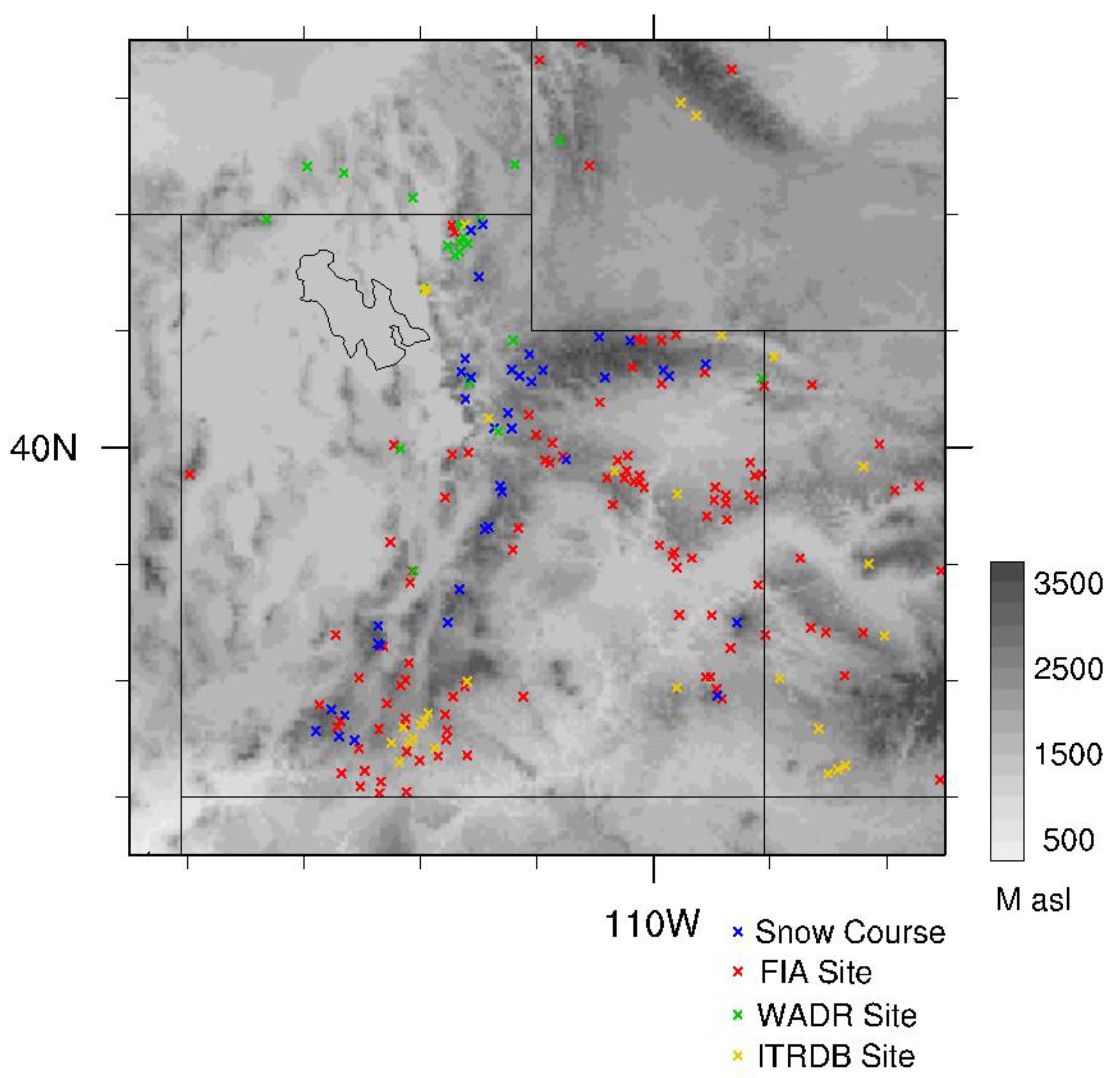
Figure 2.
April 1 SWE vs. elevation in Utah. Bold black points show the mean value for each snow course, and grey points show the individual measurements. The solid line is the linear regression of the mean snow course values with respect to elevation; the regression function is shown in the top left.

Figure 3.
Sample regridded April 1 SWE. Red points indicate the locations of snow courses, green points indicate the locations of dummy observations used in zero-padding conditioning prior to Cressman interpolation.
Figure 3.
Sample regridded April 1 SWE. Red points indicate the locations of snow courses, green points indicate the locations of dummy observations used in zero-padding conditioning prior to Cressman interpolation.
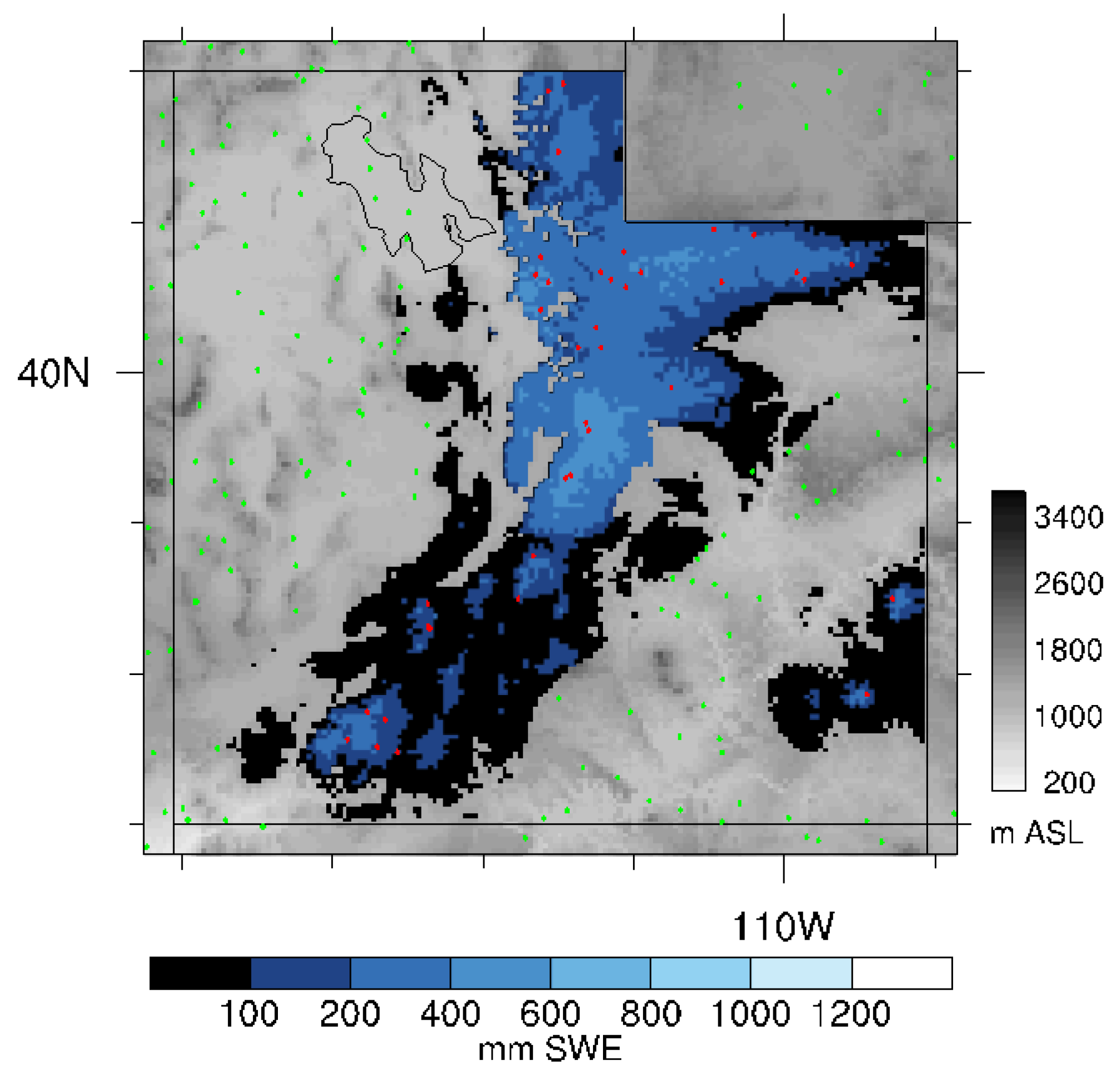
Figure 4.
Point-to-point R2 map of reconstructed-to-observed April 1 SWE, (a) including and (b) excluding FIA tree-ring data. Red points are snow courses.
Figure 4.
Point-to-point R2 map of reconstructed-to-observed April 1 SWE, (a) including and (b) excluding FIA tree-ring data. Red points are snow courses.

Figure 5.
(a) EOF 1 for NADA; (b) EOF 1 for FIA; (c) PC1 of reconstructed SWE for (a,b) (solid: FIA, dashed: NADA); and (d) spectral power of FIA PC1. In (d), the red line depicts the red noise spectrum and the dashed line indicates red noise exceedance at 95% confidence. (e–h) Same as (a–d) but for EOF 2 and FIA PC 2.

Figure 6.
Lagged correlation of PC1 (a) and PC2 (b) with a four-year low-pass filtered IPO. Dashed lines denote significant correlation at 95% and 99% confidence levels.
Figure 6.
Lagged correlation of PC1 (a) and PC2 (b) with a four-year low-pass filtered IPO. Dashed lines denote significant correlation at 95% and 99% confidence levels.
© 2017 by the authors. Licensee MDPI, Basel, Switzerland. This article is an open access article distributed under the terms and conditions of the Creative Commons Attribution (CC BY) license (http://creativecommons.org/licenses/by/4.0/).
Share and Cite
MDPI and ACS Style
Barandiaran, D.; Wang, S.-Y.S.; DeRose, R.J. Gridded Snow Water Equivalent Reconstruction for Utah Using Forest Inventory and Analysis Tree-Ring Data. Water 2017, 9, 403. https://doi.org/10.3390/w9060403
AMA Style
Barandiaran D, Wang S-YS, DeRose RJ. Gridded Snow Water Equivalent Reconstruction for Utah Using Forest Inventory and Analysis Tree-Ring Data. Water. 2017; 9(6):403. https://doi.org/10.3390/w9060403
Chicago/Turabian StyleBarandiaran, Daniel, S.-Y. Simon Wang, and R. Justin DeRose. 2017. "Gridded Snow Water Equivalent Reconstruction for Utah Using Forest Inventory and Analysis Tree-Ring Data" Water 9, no. 6: 403. https://doi.org/10.3390/w9060403
Note that from the first issue of 2016, this journal uses article numbers instead of page numbers. See further details here.