Simulating the Fate and Transport of Coal Seam Gas Chemicals in Variably-Saturated Soils Using HYDRUS


1
CSIRO, Adelaide, SA 5000, Australia
2
University of California Riverside, Riverside, CA 92521, USA
3
Department of Earth Sciences, Utrecht University, 3512 JE Utrecht, The Netherlands
4
NIDES Interdisciplinary Center for Social Development, Federal University of Rio de Janeiro, Rio de Janeiro 21941-901, Brazil
5
Belgian Nuclear Research Centre, 2400 Mol, Belgium
*
Author to whom correspondence should be addressed.
Water 2017, 9(6), 385; https://doi.org/10.3390/w9060385
Submission received: 16 April 2017
/
Revised: 11 May 2017
/
Accepted: 22 May 2017
/
Published: 30 May 2017
(This article belongs to the Special Issue Water and Solute Transport in Vadose Zone)
Abstract
:The HYDRUS-1D and HYDRUS (2D/3D) computer software packages are widely used finite element models for simulating the one-, and two- or three-dimensional movement of water, heat, and multiple solutes in variably-saturated media, respectively. While the standard HYDRUS models consider only the fate and transport of individual solutes or solutes subject to first-order degradation reactions, several specialized HYDRUS add-on modules can simulate far more complex biogeochemical processes. The objective of this paper is to provide a brief overview of the HYDRUS models and their add-on modules, and to demonstrate possible applications of the software to the subsurface fate and transport of chemicals involved in coal seam gas extraction and water management operations. One application uses the standard HYDRUS model to evaluate the natural soil attenuation potential of hydraulic fracturing chemicals and their transformation products in case of an accidental release. By coupling the processes of retardation, first-order degradation and convective-dispersive transport of the biocide bronopol and its degradation products, we demonstrated how natural attenuation reduces initial concentrations by more than a factor of hundred in the top 5 cm of the soil. A second application uses the UnsatChem module to explore the possible use of coal seam gas produced water for sustainable irrigation. Simulations with different irrigation waters (untreated, amended with surface water, and reverse osmosis treated) provided detailed results regarding chemical indicators of soil and plant health, notably SAR, EC and sodium concentrations. A third application uses the HP1 module to analyze trace metal transport involving cation exchange and surface complexation sorption reactions in a soil leached with coal seam gas produced water following some accidental water release scenario. Results show that the main process responsible for trace metal migration in soil is complexation of naturally present trace metals with inorganic ligands such as (bi)carbonate that enter the soil upon infiltration with alkaline produced water. The examples were selected to show how users can tailor the required model complexity to specific needs, such as for rapid screening or risk assessments of various chemicals nder generic soil conditions, or for more detailed site-specific analyses of actual subsurface pollution problems.
1. Introduction
Many agricultural, industrial, mining, cultural, environmental and other activities are leading to the production and use of an unprecedented number of chemicals, many of which are intentionally or accidently released into the environment. For example, agricultural operations now depend on a broad range of chemicals in plant and animal production such as fertilizers, pesticides, hormones, pharmaceuticals, pathogenic microorganisms, or fumigants, which have made agriculture one of the most important sources for non-point source pollution [1]. Examples of environmental problems resulting from non-agricultural activities are the disposal of brine/saline waters produced during extraction of coalbed or shale gas [2], releases from municipal or industrial landfills [3], acid mine drainage [4], contamination from nuclear activities [5,6], the formation of redox zones in organic-contaminated aquifers [7], and pollutant release from reactive permeable barriers used for aquifer remediation [8,9]). Advanced numerical models are required to evaluate the fate and transport of the different types of chemicals that are finding their way into the environment, including for risk assessments and site-specific management or remediation analyses [10].
The HYDRUS software packages [11] are among many other mathematical models [12] of varying degrees of complexity and dimensionality that have been developed over the last three to four decades for evaluating the fate and transport of various chemicals involved. The HYDRUS-1D and HYDRUS (2D/3D) computer software packages are popularly used finite element models for simulating the one-, and two- or three-dimensional movement of water, heat, and multiple solutes in variably-saturated media, respectively. The models, and their specialized add-on modules, have provided a great flexibility in simulating the transport of various solutes.
The standard HYDRUS models can be used to simulate the transport of individual solutes whose behavior is independent of that of other solutes that may be present in the soil solution, or of solutes subject to sequential first-order degradation reactions. Typical examples of the latter include heavy metals [13], radionuclides [14,15]), mineral nitrogen species [16], pesticides (e.g., [17]), chlorinated aliphatic hydrocarbons (e.g., [18]), hormones [19], antibiotics [20], and explosives [21]. While this approach has proved to be suitable for many chemicals, important environmental problems often require analyses of the coupled transport of multiple chemical species that may mutually interact, create complexed species, precipitate, dissolve, and/or could compete with each other for sorption sites. Several specialized HYDRUS add-on modules, such as UnsatChem, HP1, C-Ride, Wetland, or Fumigant, were developed to consider these more complex situations [11].
For example, the UnsatChem module [22,23] can simulate the transport and production of carbon dioxide, and the fate and transport of major ions, while also considering precipitation/dissolution of mineral phases and/or cation exchange reactions. On the other hand, the HP1 module, which was developed by coupling the HYDRUS and PHREEQC [24] models, provides much flexibility in modelling interactions of solutes with minerals, gases, exchangers and sorption surfaces based on thermodynamic equilibrium, kinetic, or mixed equilibrium-kinetic reactions [14,25]. Other specialized HYDRUS add-on modules, such as Wetland, C-Ride, and Fumigant, allow additional flexibility in addressing biogeochemical processes in wetlands [26,27,28], colloid-facilitated solute transport problems [29,30,31]), or the fate of fumigants in agricultural soils [32,33], respectively.
An important environmental application for numerical models is the evaluation of the fate and transport of various solutes involved in unconventional gas operations, such as the disposal of brine/saline waters produced during mining of coalbed (coal seam) or shale gas, the accidental release of produced water from water holding ponds, and the beneficial use of produced water for irrigation. In the case of coal seam gas hydraulic fracturing operations, many different chemicals are involved, the fate of which needs to be evaluated prior to their use to confirm negligible harm to humans and the environment [2]. These chemicals vary tremendously in terms of their chemical properties and how they may interact among themselves and/or with the environment. Their fate hence can be evaluated only using numerical models that have the capability to consider all pertinent reactions and interactions affecting these chemicals.
Our main objective with this study was to demonstrate how the HYDRUS models can be used to evaluate complex processes and interactions affecting the subsurface transport of various chemicals involved in coal seam gas extraction and water management operations. For this purpose we first briefly review the capabilities of the HYDRUS models, including their specialized add-on modules, to simulate the fate and transport of various solutes and their mutual interactions. We will limit this review to only those add-on modules that will be used subsequently for several applications of increasing complexity related to coal seam gas extraction and water management. The first application concerns an evaluation of the natural soil attenuation potential of hydraulic fracturing chemicals and their transformation products, for which we use the standard HYDRUS model. The second application involves an evaluation of the safe use of coal seam gas produced water for sustainable irrigation; for this application we used UnsatChem. The third application analyzes major ion geochemistry and trace metal transport in a soil leached with coal seam gas produced water; this application requires the HP1 module. We note that these three one-dimensional applications are intended to only briefly demonstrate the capabilities of the HYDRUS models and their add-on modules.
2. Theory
2.1. Variably-Saturated Water Flow
HYDRUS-1D numerically solves a modified form of the Richards equation, which describes one-dimensional uniform water movement in a partially-saturated rigid porous medium. The approach assumes that water flow due to thermal gradients can be neglected and that the air phase plays an insignificant role in the liquid flow process:
where h is the soil water pressure head [L], θ is the volumetric water content [L3L−3], t is time [T], x is the spatial coordinate [L], positive upward, K is the unsaturated hydraulic conductivity function [LT−1], S is a sink term (usually representing root water uptake) [L3L−3T−1], and α is the angle between the flow direction and the vertical axis (e.g., 1 for vertical flow, 0 for horizontal flow). The unsaturated soil hydraulic properties, θ(h) and K(h), in Equation (1) can be described in HYDRUS using the analytical models of Brooks and Corey [34], van Genuchten [35], Vogel and Císlerová [36], Kosugi [37], or Durner [38]. A macroscopic approach is used to model root water uptake, which can be either non-compensated or compensated and which can account for various stresses, such as the osmotic and pressure head stresses [39].
To account for preferential nonequilibrium flow, HYDRUS-1D can consider not only uniform variably-saturated flow, but also flow in dual-porosity and dual-permeability systems ([40]). Additionally, HYDRUS-1D can consider flow in both liquid and gaseous (vapor) phases, as well as flow driven by both capillary and gravitational forces as well as by thermal gradients [41]. Since these processes are beyond the scope of this paper, they will not be further discussed here.
2.2. Solute Transport Applications of the Standard HYDRUS Model
The standard HYDRUS models can simulate the fate and transport of individual solutes, or of solutes subject to relatively simple sequential first-order degradation reactions. The models, in general, assume that solutes can exist in all three phases (liquid, solid, and gaseous) and that the decay and production processes can be different in each phase. Solutes must be defined in the liquid phase (the liquid phase concentration is the primary variable in the advection-dispersion equation given below), but can be present additionally also in the solid and/or gaseous phases. Interactions between the solid and liquid phases may be described by linear or nonlinear (Freundlich or Langmuir) type equations, and can be either equilibrium or nonequilibrium. Interactions between the liquid and gaseous phases are assumed to be always linear and instantaneous. The models further assume that the solutes are transported by convective transport and dispersion in the liquid phase, as well as by diffusion in the gas phase. Hence, both adsorbed and volatile solutes, such as pesticides, fumigants and certain metals, can be considered.
The partial differential equations governing one-dimensional nonequilibrium chemical transport involved in a sequential first-order decay chain during transient water flow in a variably saturated rigid porous medium are taken as:
where c, s, and g are solute concentrations in the liquid [ML−3], solid [MM−1], and gaseous [ML−3], phases, respectively; ρ is the soil bulk density [ML−3], av is the air content [L3L−3], q is the volumetric flux [LT−1], Dw is the dispersion coefficient [L2T−1] for the liquid phase, Dg is the diffusion coefficient [L2T−1] for the gas phase, and P is a reaction/production term accounting for various biochemical reactions [ML−3T−1]. The subscript i represents the ith chain number. The reaction term Pi in Equation (2) in the standard HYDRUS model is defined as follows:
where μw, μs, and μg are first-order rate constants for solutes in the liquid, solid, and gas phases [T−1], respectively; μw', μs', and μg' are similar first-order rate constants providing connections between individual species in the decay chain, γw, γs, and γg are zero-order rate constants for the liquid [ML−3T−1], solid [T−1], and gas [ML−3T−1] phases, respectively, and ra is the root chemical uptake term [ML−3T−1], which for passive uptake is equal to the product of the sink term S in the water flow Equation (1) and the concentration of the sink term cr [ML−3]. The subscripts w, s, and g correspond with the liquid, solid and gas phases, respectively, and ns is the number of solutes involved in the chain reaction. The nine zero- and first-order rate constants in Equation (3) may be used to represent a variety of reactions or transformations including biodegradation, volatilization, and precipitation.
When the constants μw', μs', and μg' that provide connections between individual chain species are all set to zero, Equations (2) and (3) may be used to simulate the fate and transport of individual solutes, the behaviour of which is then assumed to be independent of that of other solutes that may be present in the soil solution. When these constants are nonzero, then Equation (2) for i = 1 is used to simulate the transport of a parent compound and for i > 1 the transport of daughter products. The above formulation has proved useful in modelling a broad range of chemicals, including radionuclides (e.g., [15,42]), mineral nitrogen species (e.g., [16,43,44]), pesticides (e.g., [17]), chlorinated aliphatic hydrocarbons (e.g., [18,45]), hormones (e.g., [19,46,47,48,49]), antibiotics (e.g., [20,50]), and explosives [51,52]. HYDRUS-1D at present considers up to ten solutes (five for the dual-permeability model), which either can be coupled in a unidirectional chain or are allowed to move independently of each other.
Physical nonequilibrium solute transport is accounted for in later versions of HYDRUS by assuming a two-region, dual-porosity (or dual-permeability) type formulation to partition the liquid phase into mobile (fast) and immobile (slow) regions. Chemical nonequilibrium solute transport is accounted for by assuming kinetic interactions between solutes in the liquid and solid phases. Attachment/detachment theories, including filtration theory, were included to simulate the transport of viruses, colloids, bacteria, nanoparticles, and/or nanotubes. Details about these nonequilibrium models can be found in Šimůnek and van Genuchten [53]. The above standard solute transport module of HYDRUS will be used below to demonstrate its application to evaluations of the natural soil attenuation potential of hydraulic fracturing chemicals (e.g., biocides) and their transformation products.
2.3. Solute Transport Applications of the UnsatChem Module
The UnsatChem module represents a typical example of a model with specific chemistry [54]. Such models usually are constrained to very specific applications since they are restricted to very prescribed chemical systems. On the other hand, these models can be numerically more efficient than models with generalized chemistry (e.g., the HP1 module as discussed below), since the numerical solution can then be optimized for a particular chemical system.
The UnsatChem geochemical module, which has been implemented in all 1D, 2D and 3D HYDRUS versions, considers the transport and production of CO2 and the transport of several main components (i.e., Ca2+, Mg2+, Na+, K+, SO42−, CO32−, and Cl−). CO2 concentrations are modelled since they can significantly affect soil pH and multiple chemical reactions, such as dissolution/precipitation reactions of calcite. The Unsatchem module considers most or all relevant equilibrium and kinetic geochemical reactions in such chemical systems as complexation, cation exchange, and precipitation-dissolution (e.g., of calcite, gypsum, and/or dolomite). A complete list of species in the code is given in the UnsatChem manual and in Table 3 of Šimůnek et al. [11]).
The carbon dioxide module of UnsatChem solves the convection-dispersion equation with a source term accounting for the production of carbon dioxide in soils. The major ion module of UnsatChem solves Equation (2) for the seven main components, while the gas-phase related terms and the general reaction term of Equation (2) are equal to zero. The second term on the left side of Equation (2) is also zero for components that do not undergo ion exchange or precipitation/dissolution reactions. While the aqueous complexation reactions do not affect Equation (2), cation exchange and precipitation/ dissolution reactions move a component from the liquid phase into the solid phase and vice versa. The solution of the chemical system is described in detail by [23].
Many possible applications of the Unsatchem module exist since saline waters are often used for irrigating agricultural crops in regions which either have limited water resources or an excess of saline waters (e.g., as produced in mining operations). Irrigation with saline water may potentially cause salinization and sodification of irrigated agricultural lands. Efficient irrigation and leaching management practices are thus critical in these regions to prevent soil salinization when rainfall is not sufficient to leach accumulated salts during or following irrigation. The UnsatChem module has been used in many studies to evaluate the sustainability of alternative irrigation schemes with respect to salinization and sodification processes, to assess reclamation of saline or sodic soils, and to evaluate the movement of salts after accidental releases or possible beneficial applications of saline waters resulting from mining operations (e.g., [55,56,57,58,59,60,61,62,63,64], among others). We will use the UnsatChem module later to demonstrate its potential for evaluating the use of coal seam gas produced water for sustainable irrigation.
2.4. Solute Transport Applications of the HP1 Module
The HP1 module represents a typical example of a model with generalized chemistry [54,65]. These models provide users with much more flexibility in designing particular chemical systems than models with specialized chemistry and allow them to carry out a much broader range of applications. Users then either can select species and reactions from large geochemical databases, are able to define their own species with particular chemical properties and reactions, and/or can build their own equilibrium and kinetic reaction networks.
The one-dimensional HP1 model [14,25] couples the PHREEQC geochemical program [24] with HYDRUS-1D. Its two-dimensional extension, HP2, was released in 2013 as an add-on module to HYDRUS (2D/3D) [11]. HPx, which is an acronym for HYDRUS-PHREEQC-xD (1D or 2D), is a very comprehensive simulation module for simulating (1) transient water flow, (2) the transport of multiple components, (3) mixed equilibrium/kinetic biogeochemical reactions, and (4) heat transport in one- and two-dimensional variably-saturated porous media. The HP1 and HP2 modules are suitable for a broad range of low-temperature biogeochemical reactions in water, the vadose zone and/or ground water systems, including interactions with minerals, gases, exchangers and sorption surfaces based on thermodynamic equilibrium, kinetic, or mixed equilibrium-kinetic reactions.
HP1 and HP2 allow thermodynamic equilibrium calculations for multiple chemical reactions and other features such as (1) aqueous speciation with different activity correction models (i.e., Davies, extended Truesdell-Jones, B-Dot, Pitzer, and SIT - Specific Ion Interaction Theory); (2) multi-site ion exchange sites with exchange described using different models (Gaines-Thomas, Vanselow, or Gapon); (3) multi-site surface complexation sites with non-electrostatic (e.g., the Dzombak and Morel or CD_MUSIC models), as well as different options to calculate compositions of the diffuse double layer; (4) mineralogical assemblages; (5) solid-solution reactions; and (6) gas exchange. Kinetic calculations can be used furthermore to describe mineral dissolution/precipitation reactions, non-equilibrium sorption, biogeochemical reactions (including first-order degradation networks), Monod kinetics and/or Michaelis-Menten kinetics [11].
The capabilities of HP1 were extended recently by considering diffusion of components (e.g., O2 or CO2) in the gas phase. This is important since concentrations of gas components may significantly affect various chemical reactions or their rates [66]. Additionally, an option to change the hydraulic and solute transport properties as a function of evolving geochemical state variables has been implemented [67]. For example, bacterial growth and/or clogging can affect porosity and corresponding physical properties. Similarly, precipitation/dissolution may lead to changes in porosity and corresponding changes in the soil water retention and hydraulic conductivity functions. It is now possible to account in HP1 for changes in porosity, hydraulic conductivity, tortuosity, dispersivity, and thermal properties such as thermal capacity, conductivity and dispersivity. The flexibility of the embedded BASIC interpreter permits HP1 users to define user-specific relationships between geochemical state variables and the transport properties [68].
Several recent applications have illustrated the versatility of HP1 to simulate a variety of complex reaction networks. Early applications [14,25] simulated long-term transient flow and the transport of major cations and heavy metals subject to a multi-site pH-dependent cation exchange complex and/or surface complexation in a multi-layered soil profile. A complex reaction network of mercury, which included kinetic dissolution from a mercury-containing solid or from an immobile non-aqueous liquid, as well as redox reactions and exchange with the soil air phase, implemented in HP1, allowed the identification of key processes and parameters for mercury transport in soils [69,70]). The network was applied to the treatment of mercury-contaminated soils with activated carbon [71]. CO2 production and transport in bare and planted mesocosms [72], and the effects of lime and concrete waste on vadose zone carbon cycling [73] furthermore illustrate applications to the problem of CO2 sequestration in soils. Recent applications are also in the field of colloid and colloid-affected transport, including competitive kinetic sorption on colloids [74] and accounting for the effects of water content and ionic strength on attachment at the air-water and soil-water interfaces, respectively [75]. The HP1 module will be used below to demonstrate its application to evaluating the fate and transport of major ions and trace metals in soils leached with coal seam gas produced water.
3. Applications
3.1. Standard HYDRUS-1D: Fate of Hydraulic Fracturing Chemicals During Natural Attenuation
3.1.1. Problem Definition
Bronopol is one of many biocides used to prevent bacteria growth in the subsurface. Biocides are essential components of hydraulic fracturing fluids used for unconventional gas extraction [76,77,78]. Bronopol also serves as a preservative in cosmetic products, liquid soaps, and cleaning agents [79]. Within well environments, bacteria often cause bioclogging and inhibit gas extraction, produce toxic hydrogen sulfide, and induce corrosion, which may lead to downhole equipment failure. Within the context of unconventional gas extraction, [77] found that uncharged biocides will dominate in the aqueous phase and be subject to degradation and transport, whereas charged biocides will sorb to solids and be less bioavailable. They also note that many biocides are short-lived or degradable through abiotic and biotic processes, while some may transform into more toxic or persistent compounds.
The aquatic toxicity of bronopol, often expressed in terms of the half-maximal inhibitory concentration EC50, or half-lethal concentration, LC50, has been reported for many marine and freshwater biota, as well as for aquatic birds ([80]). Microalgae are the most sensitive to bronopol (EC50 = 0.020–0.41 mg L−1), followed by oysters (EC50 = 0.42 and 0.78 mg L−1), water fleas (EC50 = 1.6 mg L−1), mysids (LC50 = 4.3 and 5.9 mg L−1), duckweed (EC50 = 38 mg L−1) and fish (LC50 = 7.5–59 mg L−1). Because of its low octonal/water ratio and high solubility in water, bronopol is not expected to bioaccumulate. Rapid hydrolysis occurs under warm and/or high pH conditions, resulting in the formation of formaldehyde (CH2O) which should also be considered in environmental hazard assessments [81].
Studies about human health effects of exposure to bronopol are not widely available, with most or all data on bronopol toxicity being limited to studies on animals. Based on these studies, estimated occupational short- and intermediate-term exposure levels and risks to workers have been calculated along with its classification as a Group E chemical (i.e., one for which there is evidence of non-carcinogenicity to humans [81]).
Substantial spills of bronopol into surface waters or streams by industries such as those that involve hydrocarbon extraction may therefore have noticeable ecotoxicological effects on aquatic species. These effects will depend, among other factors, on bronopol’s potential for degradation in natural environments.
3.1.2. Biocide Transformation Pathways and Natural Soil Attenuation Parameters
Bronopol (BNP) is relatively stable under normal/ambient environmental conditions, but very susceptible to degradation (hydrolysis) when exposed to elevated temperatures and alkaline conditions [81]. For example, bronopol has been reported to hydrolyze within 3 h at 60 °C and pH 8, producing formaldehyde, nitrosamines, 2-hydroxymethyl-2-nitropropane-1,3-diol (tris) and 2-bromo-2-nitroethanol [81,82,83,84,85]. Other degradation products have been reported also, including nitromethane and the more persistent bromonitromethane [82,86,87]. Figure 1 shows some of the degradation pathways for bronopol according to [87]. For the purpose of this study, the degradation pathway will be simplified to only three components, i.e., from bronopol (BNP) to 2-bromo-2-nitroethanol (BNE), and then to bromonitromethane (BNM). Importantly, the ecotoxicity changes along the degradation pathway, as is exemplified in Figure 2 for the algae Chlorella pyrenoidosa [87]. EC50 values decrease from BNP to BNE to BNM, with BNE and BNM being about twice and five times more toxic as BNP at 48 hrs exposure time.
The key parameters determining biogeochemical attenuation in the subsurface are the soil-water partitioning coefficient KD [L3M−1] and the first-order degradation constant µ = ln2/T1/2 (see Equation (3)), where T1/2 is the chemical’s half-life [T]. For nonpolar organic chemicals, KD is strongly related to the organic carbon in soil [88]. Organic compounds may also be sorbed onto mineral surfaces, especially when dry. When soils are moist, however, water will generally displace organic compounds from the mineral sorption sites; organic matter sorption then becomes more important than the small remaining contribution of mineral sorption [89]. Polar and ionizable organic compounds may sorb on both the mineral soil fractions and organic matter, with soil water content and pH often playing an important role [90].
For organic chemicals, KD is strongly related to the soil organic carbon content, fOC (expressed as g carbon g−1 soil); it is common practice for organic chemicals to derive KD from the organic carbon partition coefficient KOC, i.e., KD = fOC × KOC. The same dependency is true for the degradation constant µ. Generally, the higher the organic carbon content, the higher is KD and the faster is biodegradation. A higher organic carbon content favors microbiological activity, and as such also biodegradation. Organic carbon is generally highest in the soil top layers and decreases with depth. This implies that KD and µ generally decrease also with soil depth. For the polar chemicals BNP, BNE, and BNM sorption is typically described through use of the KOC parameter.
For deriving soil specific liquid-solid partitioning coefficients KD, soil organic carbon data typical of three soil types (Vertosols, Chromosols, and Sodosols) in New South Wales, Australia, were obtained from [91]. Organic carbon data decreased exponentially with depth, with a geometric mean fraction (fOC) of 0.0217 in the top 10 cm and a minimum background value of approximately 0.0014 at a depth of 150 cm. From there downwards, fOC remained more or less constant with depth. The exponentially decreasing organic carbon content with depth was approximated in HYDRUS-1D using a linearized depth-dependent organic carbon function. A summary of organic carbon partitioning coefficients KOC and aerobic degradation half-life values T1/2 obtained from a literature review is provided in Figure 3 (for further details see Supplementary Materials Table S1).
The average value of fOC in the top 10 cm (0.0217 g carbon g−1 soil) was multiplied by literature-based KOC values of the three compounds (BNP, BNE and BNM) to obtain their KD values (i.e., KD = fOC × KOC). This procedure was repeated for the other depths, leading to depth-dependent KD profiles for bronopol, 2-bromo-2-nitroethanol, and bromonitromethane. Finally, HYDRUS internally converted KD values into retardation factors Ri, given by:
where ρ is dry bulk density [ML−3], θ is soil water content [L3L−3] and KD,i the liquid-solid partitioning coefficient for linear reversible sorption [L3M−1]. Since in our case none of the compounds were volatile, and hence did not partition into the air phase, the solute transport equations given by Equation (2) simplify to
which assumes that degradation occurred only in the liquid phase.
For the solute transport simulations we assumed a 100-cm-deep soil profile with three soil layers: 0–30 cm, 30–70 cm, and 70–100 cm. The spatial discretisation was 1 cm; the dispersion coefficient was calculated based on a dispersivity of 10 cm or one tenth of the domain length, while molecular diffusion was neglected. Bulk densities for the three soil layers were 1.32, 1.42 and 1.45 g cm−3 for layers 1, 2 and 3, respectively. As an example, we used a θ value of 0.35 cm3 cm−3 and bulk density of 1.32 g cm−3 to calculate R values shown in Table 1 (representative for the top soil layer). Since the water content θ will vary with time and depth, R values are also time and depth-dependent. A summary of the solute transport parameters R and aerobic degradation half-life values T1/2 is provided in Table 1 (top soil layer values shown as example). The R and T1/2 values shown in Table 1 are based on a literature review (see Supplementary Materials Table S1) and represent values for the top 0–10 cm soil layer using the organic carbon value (fOC) of 0.0217 g g−1 as a reference. Both R and µ decreased linearly with depth according to the decrease in fOC. For this purpose, a new module was developed in HYDRUS-1D to automatically update KD and the degradation constant µ as organic carbon decreases with depth. The retardation and degradation constants are reduced by a depth-dependent function, which has a constant value of one (depth-reduction factor = 1) in the top of the soil profile (between soil surface and depth = A), then decreases linearly down to the value C at depth B. Below the depth B the reduction function has the value of C (Figure 4). The value for C is calculated as the ratio of organic carbon at depth B (typically the depth where organic carbon becomes more or less constant) to the organic carbon at depth A (i.e., the mean value between soil surface and depth A). In the hypothetical example of Figure 4, the mean organic carbon % from soil surface to depth A is 0.65, and the carbon content at depth B is 0.12. As result, C = 0.12/0.65 = 0.185.
Both mean retardation and half-life decreased within the degradation pathway (Table 1): the degradation products of BNP become more mobile (mean R values decreased from 187 to 2 and 17), and they degrade faster (mean T1/2 values decreased from 87 to 28 and 18) compared to BNP.
Simulations started with a 20 year infiltration period with solute-free water to achieve steady-state flow conditions. Next, simulations of the leaching behavior of BNP and its degradation products were carried out for a hypothetical leak of produced water from a water holding pond at a rate of 3.5 cm y−1 with a hypothetical concentration of 1 mg L−1 during a 30-year period (the average lifespan of a gas project during which water holding ponds are present). After this period, solute-free water was applied at a rate of 4 cm y−1 reflecting long-term mean recharge. For the unsaturated soil hydraulic properties we used the functions of van Genuchten [35] based on measured soil data points within the Cox’s Creek catchment, New South Wales (Supplementary Materials Table S2). Vertosols are the predominant soil type observed in 84 out of 143 soil profiles (59%) ([92]). Breakthrough curves for BNP, BNE, and BNM were produced at different depths to gain insight in the coupled processes of advective-dispersive transport, sorption, first-order degradation, and the generation of transformation products (notably BNE and BNM). The focus will be on the shallow soil depths of 2 and 5 cm as deeper in the profile concentrations became extremely small. Three combinations of sorption and degradation parameters were considered using values from Table 1: {max R, min T1/2}, {min R, max T1/2}, and {mean R, mean T1/2}. The first parameter combination with a maximum retardation and minimum half-life should result in maximum chemical attenuation of BNP as discussed in the next section. The second parameter combination uses the minimum retardation and maximum half-life, thus causing minimal attenuation for BNP. The third parameter set was expected to generate an average attenuation for BNP. The degree of attenuation of the transformation product BNE should not only depend on the value of its own parameter combination, but also on those of BNP. For BNM, attenuation depends on parameter combinations from all three chemicals.
3.1.3. HYDRUS-1D Simulation Results for the Bronopol Degradation Chain
Calculated breakthrough curves of BNP and its degradation products BNE and BNM are shown in Figure 5. The plots reveal much uncertainty in BNP concentrations owing to the large range in R and T1/2 values. The range in concentrations is much smaller for BNE and BNM owing to the smaller range of their parameters R and T1/2. For BNP, the maximum and minimum concentrations were indeed determined by the parameter combinations {min R, max T1/2}_BNP and {max R, min T1/2}_BNP, respectively (Figure 5, top). For the first degradation product of BNP (i.e., BNE), the maximum breakthrough concentrations is determined by the parameter combination {mean R, mean T1/2}_BNE (Figure 5, middle plots). This is a result of the parameter combinations of its parent BNP, where {mean R, mean T1/2}_BNP generates more BNE per unit of time than {min R, max T1/2}_BNP. Moreover, the latter parameters have a very high R value of 1170, thus causing BNP to move much slower through the soil than for the former parameters with R = 187. For BNM the sequence of high, mean and low breakthrough concentrations and their respective parameter combinations is the same as for BNE at 2 cm depth (Figure 5, bottom). For BNM at 5 cm depth, the {min R, max T1/2}_BNM parameter combination produced the lowest concentrations, while the {max R, min T1/2}_BNM parameter combination yielded the mean breakthrough curve concentrations (Figure 5, bottom). This is due to the considerably smaller T1/2 value (8.7 days) for the latter set compared to 30 days for the former set, while the R values are very similar, leading to much faster BNM degradation.
Overall the calculations demonstrate that the degradation products have consistently smaller concentrations than the parent compound, with maximum concentrations that are up to 100 times smaller than the parent source concentrations at depths of 2 to 5 cm. This demonstrates the significant natural attenuation capacity of soils as a result of sorption and biodegradation. The risk of bioaccumulation in soil or leaching to groundwater is hence very small for the conditions of this study, i.e., for a small infiltration flux approximately equal to the long-term recharge rate of several tens of mm per year at the study area. We note that the methodology developed here can be easily extended to a more systematic screening of the leaching risks of a broad range of organic compounds and different soil types.
3.2. UNSATCHEM: Optimizing Coal Seam Gas Produced Water for Sustainable Irrigation
3.2.1. Problem Definition
The second example considers coupled processes of variably-saturated water flow, plant water uptake and the simultaneous transport of multiple major ions in soils irrigated with produced coal seam gas water featuring different water qualities. By coupling major ion soil chemistry to unsaturated flow and plant water uptake, and by explicitly incorporating the effects of salt concentrations on soil hydraulic properties and root water uptake (salinity stress), critical soil processes required for a salinity risk assessment associated with coal seam gas produced water can be included in the analysis. Simulations with different irrigation water qualities provide detailed insight regarding chemical indicators of soil and plant health, i.e. Sodium Adsorption Ratio (SAR), EC and sodium concentrations. We compare such indicators in the soil profile with permissible soil quality guideline values in Australia (ANZECC values—[93]) to assess the risk to soil and plant health. Insights from modelling may be used to provide a scientific basis for defining safe water quality requirements for sustainable irrigation with coal seam gas produced water.
Produced water from unconventional gas extraction is generally unsuitable for direct surface discharge or irrigation without any treatment or amendment [94,95,96]. While high sodium concentrations cause soil particles to disperse, particularly if montmorillonite clays are present, most ions increase the aggregation of soil particles [96]. Irrigation water with a high SAR can therefore lead to a decrease in infiltration and deterioration of the soil structure as the dispersed clay minerals, once dry, cause soils to become dense, cloddy and structureless, thereby destroying natural particle aggregation. For example, SAR values between 5 and 8 have been shown to cause irreversible plugging of soil pores and swelling [97]. Furthermore, SAR values greater than 13 pose a risk to the soil ecosystem [94]. Typical treatments to mitigate the effects of saline-sodic irrigation water include the addition of gypsum and elemental sulphur [21,98].
The above problems can be addressed with HYDRUS using three approaches. One approach would be to use the standard HYDRUS models (similar to the bronopol example) by assuming that salinity behaves more or less like an inert tracer and hence is not subject to chemical reactions (e.g., [43]). A second approach is to use the UnsatChem module (the current example), which considers the transport and reactions between major ions (e.g., [44,56]). While the former approach does not permit such processes as cation exchange, dissolution of mineral amendments (e.g., gypsum or calcite) or precipitation of these minerals when the soil solution becomes oversaturated, the latter approach allows one to consider those geochemical processes and the effects of salts and soil water quality on soil properties and plant water uptake. Finally, a third approach would use the coupled HYDRUS-PHREEQC code [14,25], which provides users with an even greater suit of dissolved chemical species, mineral phases, and biogeochemical reactions relevant to multi-component transport (see the third example of this paper).
3.2.2. Soil Hydraulic and Chemical Model for Major Ion Transport
Three different chemical compositions of irrigation water were assumed (Table 2): (1) untreated produced water, (2) 3:1 produced water amended with surface water, and (3) produced water treated with reverse osmosis (RO). The untreated and treated compositions represent end-members that can be mixed in different ratios to obtain fit-for-purpose irrigation water. Unlike the amended and treated waters, which have actually been field-tested and/or have been used in commercial irrigation schemes, the untreated water would almost certainly not receive any permission for use as irrigation water owing to its high potassium and SAR values (Table 2). The untreated water is included in this study to demonstrate the effects of several interacting processes and identification of tipping points, such as what soil solution composition may trigger a reduction in the soil hydraulic conductivity, which then would modify water redistribution in the soil profile and impact on root water uptake. We note that the treated water is still much more saline than rainfall (e.g., Na concentrations are 60 times higher than in rainfall, Table 2). Irrigation with RO treated produced water hence is likely to have some minor effects on the soil’s chemical balance.
The same 100-cm-deep soil profile is used as in the previous example, i.e., having three soil horizons (0–30 cm, 30–70 cm, and 70–100 cm), the same van Genuchten soil hydraulic properties, and the same dispersion coefficient. Initial concentrations of the soil exchangeable cations were taken from a lysimeter located near Narrabri in northern New South Wales [100] of which the soil was characterised as a Haplic Grey Vertosol. The bulk density ranged from 1.32 to 1.45 g cm−3 for different soil depths [100]. The cation exchange capacity and the concentration of exchangeable cations of the first layer were assigned to all three horizons. The initial soil solution composition was defined by using the chemical composition of rainwater [99], which in the UnsatChem module is automatically equilibrated with the cation exchange complex.
The following hypothetical irrigation scheme was used for evaluating the potential build-up of major ions for three different irrigation water qualities: over each 5-day period, 6 cm of irrigation was applied on the first day followed by 4 days without irrigation; this resulted in a total of 73 irrigation days out of a simulation period of 365 days. Potential evapotranspiration (ET) was assumed to be 1 cm day−1 (based on the average from January 2014 in Narrabri, Australia [101]), and divided into potential evaporation (0.2 cm day−1) and potential transpiration (0.8 cm day−1). For each 5-day period, this yielded an irrigation excess of 20% above the potential ET for each day.
In our calculations we did not consider any rainfall. While this is a simplification of the soil hydrological balance and neglects the effects of rainfall salinity or salt leaching on the salt mass balance, it does allow us to focus on the effects of irrigation only using coupled chemical-hydrological-biological processes. A 50-cm-deep root zone for pasture was assumed, with the root distribution decreasing linearly with depth. Soil water and chemical mass balances were calculated for one year. Unsaturated water flow was solved using Equation (1) and accounted for water uptake by grass. The volume of water removed from a unit volume of soil per unit time due to plant water uptake, S(h) [day−1], is defined as [11]:
where α(h) is the plant-water stress response function (between 0 and 1), b(z) is the normalized water uptake distribution [cm−1] (here assumed linearly decreasing with depth), and Tp is potential transpiration [cm day−1]. At the soil surface b = 0.04 cm−1 and S(h) = 0.032 day−1.
Four modelling scenarios were considered using the Unsatchem major ion chemistry module of HYDRUS to calculate concentrations of major ions (Ca, Mg, Na, K, alkalinity, Cl, SO4), SAR, and EC in the soil profile. We used for these calculations the chemical compositions of the untreated, amended and RO-treated produced waters from Australian coal basins shown in Table 2. The first scenario uses untreated produced water, while the effects of solution composition on soil hydraulic conductivity are ignored. This scenario allows us to demonstrate the errors made when using models that do not account for solution-driven impacts on hydraulic conductivity. In Table 2 the electrical conductivity contribution of each ion (%ECi) to the total EC of the solution was calculated as ([102]):
where Ʌi is molar conductivity (S cm2 mol−1) and mi is concentration (mol L−1). Note this is approximate as Equation (8) is valid for ions at trace concentrations.
For the second scenario we used untreated produced water at a lower 4 cm day−1 irrigation rate to avoid water ponding due to reduced hydraulic conductivity. This in contrast to the initial calculations for which the 6 cm day−1 irrigation rate did not lead to ponding (results not shown). This second scenario and all further scenarios account for possible reductions in the hydraulic conductivity due to the solution composition, based on the approach of McNeal [103,104]. The third scenario uses surface water-amended produced water (at a 3:1 surface water: produced water ratio), again for a 6 cm day−1 irrigation rate. This last scenario considers RO treated produced water using the chemical composition shown in Table 2. The second, third and fourth scenarios all involved the same coupled processes, such as water balance calculations that account for root water uptake along with multiplicative water and solute stresses.
3.2.3. UNSATCHEM Simulation Results
When untreated water was used for irrigation (Scenario 2), the simulated SAR and EC evolutions showed high SAR values of over 100 (Figure 6a) and EC values exceeding 10 dS m−1 by the end of the simulation period (Figure 7a). The ANZECC SAR guide value of 20 for sand-sandy loam soil was exceeded across the entire soil profile, from the very start of the irrigation. The EC ANZECC trigger value of 0.65 dS m−1 was also exceeded quickly after irrigation started, i.e., from the surface down to 50 cm after 60 days. The rate at which SAR moves through soil is determined by the transport of Na, Ca, and Mg. The electrical conductivity (Figure 7a) progressed much faster than SAR (Figure 6a) because it is mainly determined by mono-charged sodium (54%) and the non-reactive and faster moving chloride (22%) and alkalinity (22%) (Table 2). The EC reached nearly 6 dS m−1 at the bottom of the profile after 365 days (Figure 7a), while after 365 days the SAR front (SAR up to 100) was between 30 and 40 cm depth (Figure 6a).
Using amended water (Scenario 3), the resulting SAR profiles shown in Figure 6b demonstrate that the SAR ANZECC trigger value (SAR = 20) for sand-sandy loam was exceeded after 365 days, but only in a small section of the profile. The SAR ANZECC trigger value (SAR = 5) for light clay was exceeded in the top 30 cm after 150 days, whereas after 365 days it was exceeded in the top 50 cm. The EC ANZECC trigger value of 0.65 dS m−1 was exceeded in the entire soil profile after 90 days (Figure 7b). The relatively high EC was due to the (still relatively high) EC of the irrigation water (1.57 dS m−1 or 1570 μS cm−1, Table 2). In terms of contributions of individual ions in the amended irrigation water to the EC, Table 2 shows that the most important contributors to EC were sulfate (a 36% contribution to total EC), sodium (a 26% contribution to total EC) and chloride (a 23% contribution). Optimization of irrigation water quality can be done by reducing concentrations of those ions that contribute most to the total EC. In the above example the decreasing order of importance was sulfate, sodium, and chloride.
When RO-treated water was used (Scenario 4) the simulated SAR profiles remained below the lowest SAR ANZECC trigger value of 5 for light clay (Figure 6c). This result was expected given the low SAR value (i.e., 1.6) of the irrigation water and the absence of any initial salt build-up in the soil profile (the initial SAR value was 1.25 throughout the entire soil profile) or without other salt inputs into the profile (e.g. from saline shallow groundwater or lateral inflow from water discharging at the break-of-slope [105]). The EC ANZECC trigger value of 0.65 dS m−1 was not exceeded across the entire soil profile, except at the very top few centimeters (Figure 7c). Although the EC of the irrigation water was low (0.29 dS m−1 or 290 μS cm−1, Table 2), the EC in the top of the soil profile increased to a maximum value of 0.73 dS m−1 due to evapotranspiration, leading to dry soil conditions and triggering salts to concentrate near the soil surface. In terms of contributions of individual ions in the treated irrigation water to the EC, the most important contributors were chloride (a 49.6% contribution to total EC), sodium (21.5%) and magnesium (11.3%), as shown in Table 2.
The next sections discuss the effect of different irrigation water qualities on the soil water balance components of evaporation, plant transpiration (actual and potential) and net drainage. Cumulative actual evaporation (Figure 8a) reached its maximum value of 73 cm (based on a 0.2 cm day−1 potential evaporation rate) in all scenarios except Scenario 3. The latter scenario yielded 69 cm or 95% of the potential value owing to the reduced infiltration, thereby generating drier soil moisture conditions and hence less evaporation.
Cumulative actual transpiration is a useful metric to evaluate the combined effects of soil chemical and physical processes on the soil water balance and plant water stress. The cumulative actual transpiration of all scenarios was less than its potential value (292 cm); for Scenarios 3 and 4, transpiration reached 281 cm or 96% of the potential value (Figure 8b). The plants were found to experience a very little water stress despite being irrigated with amended and treated produced water, which is most likely due to the sub-optimal irrigation regime generating soil water pressure heads slightly outside the optimal range, especially near the more negative soil pressure heads where the limiting pressure head becomes exceeded. Larger differences between actual and potential transpiration occurred for Scenarios 1 (82% of the potential value) and 2 (64% of potential value). For Scenario 1 we used the combined effects of water stress and solute stress—in combination with the major ion chemistry module—to control root water uptake. This modeling approach caused additional stress on plant water uptake, mainly due to salinity stress (the irrigation water EC was 5700 µS cm−1). The lower actual transpiration rate for Scenario 2 (188 cm) was due in part to (i) increased water stress as a result of a drier soil (4 cm day−1 rather than 6 cm day−1 irrigation rate, every 5 days), (ii) sub-optimal pressure head conditions owing to a decrease in the hydraulic conductivity induced by irrigation with high salinity, thus generating near-saturated conditions within the root zone, and (iii) salinity stress (irrigation water EC = 5700 µS cm−1).
Cumulative net drainage (the difference between cumulative inflow and outflow) was identical (−84 cm) for Scenarios 3 and 4 (Figure 8c). The higher drainage rate for Scenario 1 (123 cm) was due to the reduced transpiration, thus leaving more water in the soil profile for possible gravity drainage. The much lower drainage rate for Scenario 2 (29 cm) was a result of the smaller irrigation rate. Note that the decrease in irrigation by ~33% resulted in a decrease in drainage of approximately 65%.
The cumulative actual surface and bottom fluxes shown in Figure 8 reveal that the use of lower salinity irrigation water (Scenarios 3 and 4) produced significantly less salinity stress in that the actual transpiration rate (280 cm) was nearly equal to its potential value (292 cm), 41 cm more than for Scenario 1 (untreated water) and 93 cm more than for Scenario 2 (untreated water with possible reductions in the hydraulic conductivity). As a result, drainage from the bottom of the soil profile for Scenarios 3 and 4 was 39 cm lower than for Scenario 2 (for the same amount of irrigation water). Scenarios 3 and 4 hence were more efficient in terms of applied irrigation water use.
Similar important conclusions about the practical implications of salinity management were obtained in several earlier studies, such as by [43,61]. Ref. [61] used the UnsatChem module to demonstrate that leaching requirements would be lower when estimated with a transient modelling approach than when using a more standard steady-state model. Adopting leaching requirements based on the transient approach would hence lead to significant savings in terms of irrigation water volumes. Ref. [43] showed that while the conventional or water balance approach for estimating leaching fractions predicts little or no leaching when applied water levels are less than potential ET, field data and HYDRUS modelling showed considerable leaching around the drip lines. Spatially varying soil wetting patterns during drip irrigation causes localized leaching near the drip lines [43], thus allowing for more profitable production of various crops (e.g., processing tomato) as compared with other irrigation methods.
3.3. HP1: Trace Metal Transport in Soil Leached with Coal Seam Gas Produced Water
3.3.1. Problem Definition
Our third example uses the coupled one-dimensional HYDRUS-PHREEQC program, or HP1 [14,25], to simulate the leaching through soil of an accidental spill of produced water containing a complex mixture of inorganic chemicals and trace metals such as Cd, Cu, Pb, and Zn. The hypothetical example uses the same soil hydraulic data and dispersion coefficient as the first example, supplemented with appropriate soil chemical information to allow for the use of all geochemical capabilities of PHREEQC. Sorption processes in the soil were modelled by a combination of ion exchange and surface complexation. For details about coupling transport and reaction equations the reader is referred to [14,25].
3.3.2. Soil Geochemical Model for Trace Metal Transport
To estimate the soil’s sorption capacity associated with all relevant sorption processes, the following assumptions were made. The total sorption capacity was split in equal amounts between adsorption sites on the surface complex and adsorption sites on the cation exchanger (Table 3). This assumption was made since no information was available about the contribution of surface complexation to the total sorption capacity.
The total sorption capacity was obtained from CEC measurements on a soil profile characterised as a Haplic, Self-mulching, Grey Vertosol, in northern New South Wales, Australia [100]. The adsorption sites of the major cations were calculated based on analytical data of a lysimeter study by [100], and are summarized in Table 3. The total sorption capacity of 0.147 mol kg−1 was divided in two equal fractions (i.e., 0.074 mol kg−1 each), with fraction 1 assigned to the ion exchange sites and fraction 2 to the surface complexation sites associated with the weight% of Fe2O3 in the soil. For use of the sorption capacity in HP1, units were converted from mol·kg−1 to mol dm−3 soil. The cation exchange capacity of 0.184 mole charge dm−3 soil (for details, see Supplementary Materials) and the surface complexation capacity of 0.098 mole charge dm−3 soil (obtained by multiplying 0.074 mol kg−1 soil with bulk density) were used as input to the HP1 biogeochemical model.
The following steps were undertaken to build the soil geochemical model: (1) define initial concentrations of the trace metals Cd, Cu, Pb, U, and Zn on the sorption complex of the soil (Cu and Zn were included since they are potentially important competitors for sorption sites), and (2) define initial pore-water concentrations of all relevant chemical species (major ions and trace metals).
Adsorbed trace metal concentrations prior to the start of the leaching process were based on measurements of naturally occurring soil trace metals obtained from a geochemical survey in the study area [106]. The mobile metal content was determined using the MMI™ technology, which strips the MMI™ geochemistry mobile metal ions from the surface of soil particles using partial dissolution [106]. Figure 9 shows minimum, median, and maximum concentrations of the 17 most abundant elements (out of a total of 41 elements measured) based on 79 soil samples. Not all of the 17 most abundant elements were included in the current analysis; manganese and iron, for instance, were excluded to simplify calculations, even though they exhibited the 3rd and 4th highest adsorbed concentration. This implied a simplification in the soil geochemical model, which needs further corroboration in future studies. Calculated concentrations of the main naturally occurring trace elements of interest (Cd2+, Cu2+, Pb2+, UO22+, Zn2+) on the adsorption complex are available from Table S3.
Next, the initial concentrations of all relevant chemical species on the cation exchanger were used to define an initial pore-water solution prior to infiltration of the leachate solution. The geochemical model defines initial concentrations as follows:
Step 1: All initial concentrations of major cations (Table 3) and trace metals (Table S3) are assigned to the cation exchanger;
Step 2: Mixing with an initially solute-free pore-water solution takes place to define an initial pore-water solution with cations and trace metals;
Step 3: Rainwater is allowed to infiltrate, causing the pore-water solution and the rain water to equilibrate with the surface complex and the cation exchanger.
The initial pore-water solution from Step 2 was mixed with a boundary solution typical of rainwater [99] to achieve a steady-state chemical profile within the soil. In defining the chemical composition of rainfall, with a total annual rainfall of 70 cm y−1 and an estimated recharge of 4 cm y−1, concentrations in rainwater were converted to concentrations in recharge water by multiplying the former by the ratio of rainfall to recharge, i.e., 70/4 or 17.5. In this way, the effect of “concentration” of solutes in the top of the profile was accounted for.
The second boundary solution was defined by the composition of the produced water that was considered to infiltrate in the soil as a result of a hypothetical accidental leak from a water holding pond. Three different compositions of produced water were available from three different sites. For our example we used the composition of Site 3 (Figure 10).
A total of 18 components (Cl, Ca, Mg, Na, K, Al, C(4), S(6), F, Cd, Zn, Pb, Cu(1), Cu(2) U(5), U(6), H, O) were transported in the model. Although this number simplifies the composition of produced water, the simplification is justified since other components such as phosphate and nitrate had low to very low concentrations in the produced water. Table 4 lists, as an example, the aqueous phase species for lead since this element will be the focus of our discussion later; the remaining trace metal aqueous phase species for Cd, Cu, U and Zn are available from Table S4. The cation exchange and surface complexation species considered in the geochemical model are shown in Table 5 and Table 6, respectively.
The following three scenarios are considered illustrative examples of multi-component trace metal transport in soil following a long-term leak from a water holding pond:
Scenario 1 assumes rainwater infiltration only with a flux of 4 cm y−1 over a 100 year period, and with a rainwater chemical composition as given in Table S5. This allows a comparison of soil geochemical behaviour under natural conditions of rainwater infiltration with the scenarios of infiltration of produced water with a very specific hydrochemistry (Scenarios 2 and 3).
Scenario 2 considers infiltration of produced water from which trace metals were excluded, thus keeping only major ions (site 3, Figure 10). This analysis was undertaken to evaluate trace metal behaviour in soils where the naturally present adsorbed trace metals (the background concentration shown in Figure 9) were exposed to an infiltrating alkaline solution (the produced water infiltrating the soil has a pH of 9.14). This provides a basis for comparisons with trace metal behaviour when metal-containing produced water infiltrates.
Scenario 3 includes all measured trace metals in the produced water infiltrating the soil (site 3, Figure 10).
To simplify the interpretation of trace metal chemical behavior, a 100-cm deep soil profile with a single soil material was considered, with the soil hydraulic properties of layer 1 from Table S2. The profile was discretized into 100 equidistant finite elements. Soil sorption was hypothesized to consist of 50% adsorption sites with surface complexation and 50% adsorption sites with cation exchange. The cation exchange and surface complexation capacities are summarised in Table 3. Time-variable top boundary conditions were defined as follows: the first period consisted of 100 years of rainwater infiltration during which a water holding pond was absent, with the chemical composition of the rainwater defined in Table S5. After this initial “warming up” period that allows chemical equilibration between soil and rainwater to be established, the actual infiltration of produced water took place over a 30-year period during which a water holding pond was present and leaked at a very small rate of 0.35 cm y−1. The chemical composition of the Site 3 produced water was used as input to the simulations (Figure 10). The last period was defined by infiltration of rainwater for another 70 years, thus assuming that the water holding pond had been dismantled, using the same chemical composition as the initial warming-up period. The rainwater infiltration flux was always 4 cm y−1.
3.3.3. HP1 Simulation Results
The discussions below focus on the following aspects from the wealth of output provided by the HP1 simulations: (i) changes in adsorbed concentrations of lead on the cation exchanger and the surface complex, (ii) changes in liquid phase concentrations for the same trace metal, and (iii) changes in trace metal fluxes at the bottom of the 1-m deep soil profile. The detailed analysis of the trace metal behavior uses eight time steps at which adsorbed and aqueous phase concentrations are plotted. The time corresponding to 100 years of rainwater infiltration, after which equilibrium in chemistry between rainwater and soil water was established, was defined as t0. Chemical concentrations within the soil profile at t0 represented steady-state conditions for Scenario 1. Three time steps (10 [t10], 20 [t20], and 30 years [t30]) were defined to capture changes during the 30-year infiltration period with produced water. To evaluate the progression of chemical leaching once infiltration with produced water terminated and rainwater infiltrated again (from t > 30 to t = 100 years), short (5-year) time steps t35, t40 and t45 were used to capture changes that would occur within 15 years of rainfall infiltration. The final time level t100, corresponded to the total simulation time of 200 years, i.e. 100 years after the start of the infiltration of produced water.
Scenario 1 is represented by a single curve (i.e., the initial concentration at t0) in Figure 11 and Figure 12). The effect of infiltration with produced water (Scenarios 2 and 3) produced less adsorbed lead on the cation exchanger and the surface complexation sites (Figure 12), which in turn decreased aqueous lead owing to equilibrium between the solid and liquid phase concentrations (Figure 11). At the end of the simulation (t100), re-adsorption of lead occurred on both adsorption sites between depths of 0.4 and 1 m. The lower liquid phase concentration at t100 is a reflection of the mass loss of lead from the adsorption sites; and the equilibrium partitioning of lead between solid and liquid phase according to the equations in Table 5 and Table 6.
A comparison between Scenarios 2 (infiltration with metal-free water) and 3 (infiltration with metal-containing water) shows no significant difference in lead concentrations in the soil profile, neither for the liquid (Figure 11) or adsorbed phase (Figure 12). Most of the total adsorbed lead resided on the surface complex before and during infiltration of the produced water; some desorption from the surface complex is noticeable close to the surface (Figure 11). Strong desorption of Pb occurred on the cation exchanger, with only slow re-adsorption after t30. The concentration in the liquid phase initially increased to a maximum of about 10−7 mol L−1 up to 0.5 m depth at t30 (due to desorption of Pb from the cation exchanger), then decreased again due to leaching with rainwater such that at t100 Pb was removed from the pore-water with final concentrations smaller than at those at t0. (Figure 11).
Our findings indicate that the main processes of trace metal sorption, desorption and transport are not linked to metals present in the produced water. The observed concentration distributions are the result of complexation reactions between inorganic compounds present in the alkaline produced water and the trace metals present on the solid phases prior to infiltration. To evaluate which dissolved species from the infiltrating solution are responsible for the desorption and transport of trace metals (for a full list of lead species considered, see Table 4), and how they affect the dynamics of trace metal sorption/desorption during the leakage period, the most abundant liquid phase lead species at t0 and at t25 are displayed in Figure 13. To appreciate the results, changes in the pH also need consideration: there is generally a significant increase in solution pH from initial values around 7.2–7.4 to nearly 9.
Prior to infiltration with produced water (at t0), about 60% of all dissolved lead species were represented by the cation Pb2+, about 20% by the cation PbOH+, and approximately 15–20% by the neutral PbCO3 (Figure 13). Smaller fractions were due to the species Pb(CO3)22−, PbHCO3+, PbSO4, and PbCl+. After infiltration with produced water (species distribution shown at t25), the maximum percentage for Pb2+ had decreased to 20%. The predominant species was then the neutral species PbCO3 with a maximum percentage of approximately 80%. Furthermore, the abundance of two other carbonate species (Pb(CO3)22−, PbHCO3+) increased compared to the initial condition. These neutral and negatively charged lead species have a higher mobility than the positively charged Pb2+, causing the latter to desorb and to be transported down the profile as predominantly PbCO3, Pb(CO3)22− and PbHCO3+.
Further evidence for nearly unretarded transport of the dominant liquid phase species is found in a comparison of the solute fluxes of lead (total lead concentration based on all dissolved species) and chloride at the bottom of the soil profile. Figure 14 displays the bottom solute fluxes of total lead and chloride: the peak concentration appeared at the same time for both chemicals, i.e., 35 years after the beginning of the leakage. This confirms that the neutral or negatively charged lead species are transported unretarded through the soil profile.
We made a final comparison of lead fluxes obtained for Scenarios 2 (metal free) and 3 (metal containing) by considering the bottom fluxes of total lead at 1-m depth. As expected, no difference in the flux occurred for the two scenarios. The peak of the bottom solute flux at 1 m was reached 35 years after the start of the infiltration of produced water for both scenarios (Figure 14). This confirms that lead leaching is due to desorption of naturally present lead species following the infiltration of an alkaline solution; the contribution of trace metals, including those present in produced water, did not materially contribute to the final lead flux.
4. Summary and Conclusions
In this paper we demonstrated the use of the HYDRUS software and its specialized add-on modules UnsatChem (for major ion chemistry) and HP1 (for more general multicomponent transport) to evaluate the fate and subsurface transport of various chemicals involved in coal seam gas extraction and water management operations after their accidental or intentional release at the soil surface. The three examples we discussed represented increasing model complexity from the relatively standard HYDRUS (example 1), to using the UnsatChem module (example 2), and finally HP1 (example 3).
The first example evaluated the fate and transport of organic chemicals (i.e. biocide) in soil as a result of their accidental release from water holding ponds containing produced water. The standard HYDRUS software was used to simulate the coupled processes of retardation, first-order degradation and convective-dispersive transport of the biocide bronopol and its degradation products. We presented a review of degradation pathways and relevant biogeochemical processes, including a collation of physico-chemical properties of bronopol and two of its degradation products (2-bromo-2-nitroethanol and bromonitromethane) as input to a set of generic simulations of transport and attenuation in variably-saturated soil profiles. We demonstrated the ability to model the coupled processes of fluid flow and transport of multiple contaminants in soils, with a sensitivity analysis testing the robustness of contaminant migration and attenuation with regards to chemical parameters.
In a second example we used the major ion chemistry module UnsatChem to simulate the simultaneous movement of multiple major ions (Na, K, Ca, Mg, Cl, SO4, alkalinity) present in irrigation water sourced from coal seam gas produced water. This analysis illustrated the identification and potential optimisation of irrigation water quality that will minimize long-term harmful effects of dissolved ions on soil and plant health. Three different irrigation water qualities were evaluated: untreated or treated produced water or produced water amended with surface water. Simulations with the different irrigation waters provided detailed results regarding chemical indicators of soil and plant health, notably SAR, EC and sodium concentrations. By comparing these indicators in the soil profile with water quality guideline values (i.e., the Australian and New Zealand ANZECC values), an assessment could be made of the suitability of the applied produced water for long-term irrigation. The major ion chemistry module UnsatChem implemented in HYDRUS-1D also allowed for testing the effects of salinity on root-water uptake and thus on crop transpiration. The example additionally permitted calculations of the effects of salinity on the soil hydraulic conductivity and how reductions in this key soil property can lead to water logging and hence reduced root-water uptake. UnsatChem offers a cost-effective way to optimise the quality of irrigation water derived from coal seam gas water or other saline waters and thus to ensure that soils are managed in a sustainable manner.
The third example used HP1 to determine key processes contributing to the migration of naturally occurring trace metals cadmium, lead, and uranium present in a particular soil profile. Based on a discussion that focused on the trace metal lead, chemical transport and attenuation processes in soil were simulated by including adsorption of trace metals through cation exchange and surface complexation. The assessment was based on an analysis, in space and time, of adsorbed and aqueous phase metal concentrations and the relative abundance of dissolved metal species. Results show that the main process responsible for trace metal migration in soil is complexation of naturally present metals with inorganic ligands such as (bi)carbonate, chloride, and hydroxyl ions. These ligands enter the soil upon infiltration with coal seam gas produced water, which is typically alkaline (pH = 8–9). Trace metals naturally present on adsorption sites in the soil, even at low levels, may desorb due to formation of especially mobile carbonate metal-ligand compounds. These metal-ligand compounds travel relatively unretarded through soil. The multi-component reactive transport simulator HP1 was shown to be a powerful tool to assess contamination risk from release of industrial waters. The ability to incorporate coupled physical, chemical, geological and biological processes in the simulations also allows testing of mitigating measures as part of pollution prevention.
Supplementary Materials
The following are available online at www.mdpi.com/2073-4441/9/6/385/s1. Table S1: Organic carbon partition coefficient KOC (L/kg) and aerobic degradation half-lives (T1/2, days) of bronopol and two of its degradation products; Table S2: van Genuchten soil hydraulic parameters and the bulk density of Vertosols (averages across the Cox’s Creak Catchment area, NSW, Australia) (source: [7]); Table S3: Conversion of the concentrations [ppm] measured by de Caritat and Lech [9] to the initial concentrations [mol/kg] on the cation exchanger; Table S4: Aqueous phase species of the heavy metals included in the model (phreeqcU.dat database used). Table S4: Rainfall data and chemical composition of rainwater at Wagga Wagga, Australia (Source: [9]). HP1 input data calculated for an infiltration flux of 40 mm/y.
Acknowledgments
We are grateful to Boris Faybishenko (Lawrence Berkeley National Laboratory), Guest Editor of the Special Issue “Water and Solute Transport in the Vadose Zone”, for the invitation to present our paper. Thanks also to the three anonymous reviewers for their constructive comments. The first author acknowledges CSIRO Land and Water for funding received through the strategic appropriation research project “Next generation methods and capability for multi-scale cumulative impact and management”.
Author Contributions
Dirk Mallants collated the data and performed the simulations; Dirk Mallants, Jirka Šimůnek, Martinus Th. van Genuchten and Diederik Jacques contributed to the writing of the paper.
Conflicts of Interest
The authors declare no conflict of interest.
References
- Singh, G.; Kaur, G.; Williard, K.; Schoonover, J.; Kang, J. Monitoring of Water and Solute Transport in the Vadose Zone: A Review. Vadose Zone J. 2017. [Google Scholar] [CrossRef]
- US EPA. Hydraulic Fracturing for Oil and Gas: Impacts from the Hydraulic Fracturing Water Cycle on Drinking Water Resources in the United States; Office of Research and Development: Washington, DC, USA, 2016; EPA/600/R-16/236Fa.
- Christensen, T.H.; Kjeldsen, P.; Bjerg, P.L.; Jensen, D.L.; Christensen, J.B.; Baun, A.; Albrechtsen, H.-J.; Heron, G. Biogeochemistry of landfill leachate plumes. Appl. Geochem. 2001, 16, 659–718. [Google Scholar] [CrossRef]
- Akcil, A.; Koldas, S. Acid mine drainage (AMD): Causes, treatment and case studies. J. Clean. Prod. 2006, 14, 1139–1145. [Google Scholar] [CrossRef]
- Fredrickson, J.K.; Zachara, J.M.; Balkwill, D.L.; Kennedy, D.; Li, S.-M.W.; Kostandarithes, H.M.; Daly, M.J.; Romine, M.F.; Brockman, F.J. Geomicrobiology of High-Level Nuclear Waste-Contaminated Vadose Sediments at the Hanford Site, Washington State. Appl. Environm. Microbiol. 2004, 70, 4230–4241. [Google Scholar] [CrossRef] [PubMed]
- Vandenhove, H.; Sweeck, L.; Mallants, D.; Vanmarcke, H.; Aitkulov, A.; Sadyrov, O.; Savosin, M.; Tolongutov, B.; Mirzachev, M.; Clerc, J.J.; et al. Assessment of radiation exposure in the uranium and milling area of Mailuu Suu, Kyrgyzstan. J. Environ. Radioact. 2006, 88, 118–139. [Google Scholar] [CrossRef] [PubMed]
- Lapworth, D.J.; Baran, N.; Stuart, M.E.; Ward, R.S. Emerging organic contaminants in groundwater: A review of sources, fate and occurrence. Environ. Pollut. 2012, 163, 287–303. [Google Scholar] [CrossRef] [PubMed]
- Mallants, D.; Diels, L.; Bastians, L.; Vos, J.; Moors, H.; Wang, L.; Maes, N.; Vandenhove, H. Removal of Uranium and Arsenic from Groundwater Using Six Different Reactive Materials: Assessment of Removal Efficiency. In Uranium in the Aquatic Environment; Merkel, B.J., Planer-Friedrich, B., Wolkersdolfer, C., Eds.; Springer: Berlin, Germany, 2002; pp. 561–568. [Google Scholar]
- Scherer, M.M.; Richter, S.; Valentine, R.L.; Alvarez, P.J.J. Chemistry and microbiology of permeable reactive barriers for in situ groundwater clean up. Crit. Rev. Environ. Sci. Technol. 2000, 30, 363–411. [Google Scholar] [CrossRef]
- Šimůnek, J.; Jacques, D.; Langergraber, G.; Bradford, S.A.; Šejna, M.; van Genuchten, M.T. Numerical Modelling of Contaminant Transport Using HYDRUS and Its Specialized Modules, Invited paper for the Special Issue “Water Management in Changing Environment”. J. Indian Inst. Sci. 2013, 93, 265–284. [Google Scholar]
- Šimůnek, J.; van Genuchten, M.T.; Šejna, M. Recent developments and applications of the HYDRUS computer software packages. Vadose Zone J. 2016, 15, 25. [Google Scholar] [CrossRef]
- Šimůnek, J.; Bradford, S. Vadose Zone Modelling: Introduction and importance. Vadose Zone J. 2008, 7, 581–586. [Google Scholar] [CrossRef]
- Seuntjens, P.; Mallants, D.; Šimůnek, J.; Patyn, J.; Jacques, D. Sensitivity analysis of physical and chemical properties affecting field-scale cadmium transport in a heterogeneous soil profile. J. Hydrol. 2002, 264, 185–200. [Google Scholar] [CrossRef]
- Jacques, D.; Šimůnek, J.; Mallants, D.; van Genuchten, M.T. Modelling coupled hydrologic and chemical processes: Long-term Uranium transport following Phosphorus fertilization. Vadose Zone J. 2008, 7, 698–711. [Google Scholar] [CrossRef]
- Mallants, D.; Jacques, D.; Zeevaert, T. Modelling 226Ra, 222Rn, and 210Pb Migration in a Proposed Surface Repository of Very Low-Level Long-Lived Radioactive Waste. In Proceedings of the ICEM 2003, the 9th International Conference on Radioactive Waste Management and Environmental Remediation, Oxford, UK, 21–25 September 2003; icem03-4632. p. 8. [Google Scholar]
- Li, Y.; Šimůnek, J.; Zhang, Z.; Jing, L.; Ni, L. Evaluation of nitrogen balance in a direct-seeded-rice field experiment using Hydrus-1D. Agric. Water Manag. 2015, 148, 213–222. [Google Scholar] [CrossRef]
- Papiernik, S.K.; Yates, S.R.; Koskinen, W.C.; Barber, B. Processes affecting the dissipation of the herbicide isoxaflutole and its diketonitrile metabolite in agricultural soils under field conditions. J. Agric. Food Chem. 2007, 55, 8630–8639. [Google Scholar] [CrossRef] [PubMed]
- Schaerlaekens, J.; Mallants, D.; Šimůnek, J.; van Genuchten, M.T.; Feyen, J. Numerical simulation of transport and sequential biodegradation of chlorinated aliphatic hydrocarbons using CHAIN_2D. Hydrol. Proc. 1999, 13, 2847–2859. [Google Scholar] [CrossRef]
- Fan, Z.; Casey, F.X.M.; Hakk, H.; Larsen, G.L. Discerning and modelling the fate and transport of testosterone in undisturbed soil. J. Environ. Qual. 2007, 36, 864–873. [Google Scholar] [CrossRef] [PubMed]
- Unold, M.; Šimůnek, J.; Kasteel, R.; Groeneweg, J.; Vereecken, H. Transport of manure-based applied sulfadiazine and its main transformation products in soil columns. Vadose Zone J. 2009, 8, 677–689. [Google Scholar] [CrossRef]
- Šimůnek, J.; Jacques, D.; van Genuchten, M.T.; Mallants, D. Multicomponent geochemical transport modelling using Hydrus-1D and HP1. J. Am. Water Resour. Assoc. 2006, 42, 1537–1547. [Google Scholar] [CrossRef]
- Šimůnek, J.; Suarez, D.L. Two-dimensional transport model for variably saturated porous media with major ion chemistry. Water Resour. Res. 1994, 30, 1115–1133. [Google Scholar] [CrossRef]
- Šimůnek, J.; Suarez, D.L. Sodic soil reclamation using multicomponent transport modelling. J. Irrig. Drain. Eng. 1997, 123, 367–376. [Google Scholar] [CrossRef]
- Parkhurst, D.L.; Appelo, C.A.J. User’s Guide to PHREEQ C (Version 2)—A Computer Program for Speciation, Batch-Reaction, One-Dimensional Transport and Inverse Geochemical Calculations. In Water-Resources Investigations; Report 99-4259; U.S. Geological Survey: Earth Science Information Center: Denver, CO, USA, 1999; p. 312. [Google Scholar]
- Jacques, D.; Šimůnek, J.; Mallants, D.; van Genuchten, M.T. Modelling coupled water flow, solute transport and geochemical reactions affecting heavy metal migration in a podzol soil. Geoderma 2008, 145, 449–461. [Google Scholar] [CrossRef]
- Langergraber, G.; Šimůnek, J. Modelling variably-saturated water flow and multi-component reactive transport in constructed wetlands. Vadose Zone J. 2005, 4, 924–938. [Google Scholar] [CrossRef]
- Langergraber, G.; Šimůnek, J. Reactive transport modelling of subsurface flow constructed wetlands. Vadose Zone J. 2012, 11. [Google Scholar] [CrossRef]
- Langergraber, G.; Rousseau, D.; García, J.; Mena, J. CWM1—A general model to describe biokinetic processes in subsurface flow constructed wetlands. Water Sci. Technol. 2009, 59, 1687–1697. [Google Scholar] [CrossRef] [PubMed]
- Šimůnek, J.; Changming, H.; Pang, L.; Bradford, S.A. Colloid-facilitated transport in variably-saturated porous media: Numerical model and experimental verification. Vadose Zone J. 2006, 5, 1035–1047. [Google Scholar] [CrossRef]
- Pang, L.; Šimůnek, J. Evaluation of bacteria-facilitated cadmium transport in gravel columns using the HYDRUS colloid-facilitated solute transport model. Water Resour. Res. 2006, 42, W12S10. [Google Scholar] [CrossRef]
- Zhang, M.; Engelhardt, I.; Šimůnek, J.; Bradford, S.A.; Kasel, D.; Berns, A.E.; Vereecken, H.; Klumpp, E. Co-transport of chlordecone and sulfadiazine in the presence of functionalized multi-walled carbon nanotubes in soils. Environ. Pollut. 2017, 221, 470–479. [Google Scholar] [CrossRef] [PubMed]
- Spurlock, F.; Šimůnek, J.; Johnson, B.; Tuli, A. Sensitivity analysis of vadose zone fumigant transport and volatilization. Vadose Zone J. 2013, 12, 12. [Google Scholar] [CrossRef]
- Spurlock, F.; Johnson, B.; Tuli, A.; Gao, S.; Tao, J.; Sartori, F.; Qin, R.; Sullivan, D.; Stanghellini, M.; Ajwa, H. Simulation of fumigant transport and volatilization from tarped broadcast applications. Vadose Zone J. 2013, 12, 10. [Google Scholar] [CrossRef]
- Brooks, R.H.; Corey, A.T. Hydraulic Properties of Porous Media. In Hydrology Paper No. 3; Colorado State University: Fort Collins, CO, USA, 1964. [Google Scholar]
- van Genuchten, M.T. A closed-form equation for predicting the hydraulic conductivity of unsaturated soils. Soil Sci. Soc. Am. J. 1980, 44, 892–898. [Google Scholar] [CrossRef]
- Vogel, T.; Císlerová, M. On the reliability of unsaturated hydraulic conductivity calculated from the moisture retention curve. Transp. Porous Med. 1988, 3, 1–15. [Google Scholar] [CrossRef]
- Kosugi, K. Lognormal distribution model for unsaturated soil hydraulic properties. Water Resour. Res. 1996, 32, 2697–2703. [Google Scholar] [CrossRef]
- Durner, W. Hydraulic conductivity estimation for soils with heterogeneous pore structure. Water Resour. Res. 1994, 30, 211–233. [Google Scholar] [CrossRef]
- Šimůnek, J.; Hopmans, J.W. Modelling compensated root water and nutrient uptake. Ecol. Model. 2009, 220, 505–521. [Google Scholar] [CrossRef]
- Šimůnek, J.; Jarvis, N.J.; van Genuchten, M.T.; Gärdenäs, A. Review and comparison of models for describing non-equilibrium and preferential flow and transport in the vadose zone. J. Hydrol. 2003, 272, 14–35. [Google Scholar] [CrossRef]
- Saito, H.; Šimůnek, J.; Mohanty, B. Numerical analyses of coupled water, vapor, and heat transport in the vadose zone. Vadose Zone J. 2006, 5, 784–800. [Google Scholar] [CrossRef]
- Pontedeiro, E.M.; van Genuchten, M.T.; Cotta, R.M.; Šimůnek, J. The effects of preferential flow and soil texture on risk assessments of a NORM waste disposal site. J. Hazard. Mater. 2010, 174, 648–655. [Google Scholar] [CrossRef] [PubMed]
- Hanson, B.R.; Šimůnek, J.; Hopmans, J.W. Numerical modelling of urea-ammonium-nitrate fertigation under micro-irrigation. Agric. Water Manag. 2006, 86, 102–113. [Google Scholar] [CrossRef]
- Ramos, T.B.; Šimůnek, J.; Gonçalves, M.C.; Martins, J.C.; Prazeres, A.; Pereira, L.S. Two-dimensional modelling of water and nitrogen fate from sweet sorghum irrigated with fresh and blended saline waters. Agric. Water Manag. 2012, 111, 87–104. [Google Scholar] [CrossRef]
- Casey, F.X.M.; Šimůnek, J. Inverse analyses of the transport of chlorinated hydrocarbons subject to sequential transformation reactions. J. Environ. Qual. 2001, 30, 1354–1360. [Google Scholar] [CrossRef] [PubMed]
- Casey, F.X.M.; Larsen, G.L.; Hakk, H.; Šimůnek, J. Fate and transport of 17β-Estradiol in soil-water systems. Environ. Sci. Technol. 2003, 37, 2400–2409. [Google Scholar] [CrossRef] [PubMed]
- Casey, F.X.M.; Larsen, G.L.; Hakk, H.; Šimůnek, J. Fate and transport of testosterone in agriculturally significant soils. Environ. Sci. Technol. 2004, 38, 790–798. [Google Scholar] [CrossRef] [PubMed]
- Casey, F.X.M.; Šimůnek, J.; Lee, J.; Larsen, G.L.; Hakk, H. Sorption, mobility, and transformation of estrogenic hormones in natural soil. J. Environ. Qual. 2005, 34, 1372–1379. [Google Scholar] [CrossRef] [PubMed]
- Das, B.S.; Lee, L.S.; Rao, P.S.C.; Hultgren, R.P. Sorption and degradation of steroid hormones in soils during transport: Column studies and model evaluation. Environ. Sci. Technol. 2004, 38, 1460–1470. [Google Scholar] [CrossRef] [PubMed]
- Wehrhan, A.; Kasteel, R.; Šimůnek, J.; Groeneweg, J.; Vereecken, H. Transport of sulfadiazine in soil columns—experiments and modelling approaches. J. Contam. Hydrol. 2007, 89, 107–135. [Google Scholar] [CrossRef] [PubMed]
- Dontsova, K.M.; Yost, S.L.; Šimůnek, J.; Pennington, J.C.; Williford, C. Dissolution and transport of TNT, RDX, and Composition B in saturated soil columns. J. Environ. Qual. 2006, 35, 2043–2054. [Google Scholar] [CrossRef] [PubMed]
- Dontsova, K.M.; Pennington, J.C.; Hayes, C.; Šimůnek, J.; Williford, C.W. Dissolution and transport of 2,4-DNT and 2,6-DNT from M1 propellant in soil. Chemosphere 2009, 77, 597–603. [Google Scholar] [CrossRef] [PubMed]
- Šimůnek, J.; van Genuchten, M.T. Modeling Nonequilibrium Flow and Transport Processes Using HYDRUS. Vadose Zone J. 2008, 7, 782–797. [Google Scholar] [CrossRef]
- Šimůnek, J.; Valocchi, A.J. Geochemical Transport. In Methods of Soil Analysis, Part 1, Physical Methods, Chapter 6.9, 3rd ed.; Dane, J.H., Topp, G.C., Eds.; SSSA: Madison, WI, USA, 2002; pp. 1511–1536. [Google Scholar]
- Kaledhonkar, M.J.; Keshari, A.K. Modelling the effects of saline water use in agriculture. Irrig. Drain. 2006, 55, 177–190. [Google Scholar] [CrossRef]
- Gonçalves, M.C.; Šimůnek, J.; Ramos, T.B.; Martins, J.C.; Neves, M.J.; Pires, F.P. Multicomponent solute transport in soil lysimeters irrigated with waters of different quality. Water Resour. Res. 2006, 42, W08401. [Google Scholar] [CrossRef]
- Kaledhonkar, M.J.; Keshari, A.K.S.; van der Zee, E.A.T.M. Relative sensitivity of ESP profile to spatial and temporal variability in cation exchange capacity and pore water velocity under simulated field conditions. Agric. Water Manag. 2006, 83, 58–68. [Google Scholar] [CrossRef]
- Kaledhonkar, M.J.; Sharma, D.R.; Tyagi, N.K.; Kumar, A.; van der Zee, S.E.A.T.M. Modelling for conjunctive use irrigation planning in sodic groundwater areas. Agric. Water Manag. 2012, 107, 14–22. [Google Scholar] [CrossRef]
- Skaggs, T.H.; Shouse, P.J.; Poss, J.A. Irrigation of forage crops with saline drainage waters: 2. Modelling drainage and root water uptake. Vadose Zone J. 2006, 5, 824–837. [Google Scholar] [CrossRef]
- Schoups, G.; Hopmans, J.W.; Tanji, K.K. Evaluation of model complexity and space–time resolution on the prediction of long-term soil salinity dynamics, western San Joaquin Valley, California. Hydrol. Process. 2006, 20, 2647–2668. [Google Scholar] [CrossRef]
- Corwin, D.L.; Rhoades, J.D.; Šimůnek, J. Leaching requirement for soil salinity control: Steady-state vs. transient-state models. Agric. Water Manag. 2007, 90, 165–180. [Google Scholar] [CrossRef]
- Ramos, T.B.; Šimůnek, J.; Gonçalves, M.C.; Martins, J.C.; Prazeres, A.; Castanheira, N.L.; Pereira, L.S. Field evaluation of a multicomponent solute transport model in soils irrigated with saline waters. J. Hydrol. 2011, 407, 129–144. [Google Scholar] [CrossRef]
- Rasouli, F.; Pouya, A.K.; Šimůnek, J. Modelling the effects of saline water use in wheat-cultivated lands using the UNSATCHEM model. Irrig. Sci. 2013, 31, 1009–1024. [Google Scholar] [CrossRef]
- Jakubowski, R.; Haws, N.; Ellerbrock, D.; Murtagh, J.; MacFarlane, D. Development of a management tool to support the beneficial use of treated coal seam gas water for irrigation in Eastern Australia. Mine Water Environ. 2014, 33, 133–145. [Google Scholar] [CrossRef]
- Steefel, C.I.; Appelo, C.A.J.; Arora, B.; Jacques, D.; Kalbacher, T.; Kolditz, O.; Lagneau, V.; Lichtner, P.C.; Mayer, K.U.; Meeussen, J.C.L.; et al. Reactive transport codes for subsurface environmental simulation. Comput. Geosci. 2015, 19, 445–447. [Google Scholar] [CrossRef]
- Mayer, K.U.; Alt-Epping, P.; Jacques, D.; Arora, B.; Steefel, C.I. Benchmark problems for reactive transport modeling of the generation and attenuation of acid rock drainage. Comput. Geosci. 2015, 19, 599–611. [Google Scholar] [CrossRef]
- Xie, M.; Mayer, K.U.; Claret, F.; Alt-Epping, P.; Jacques, D.; Steefel, C.; Chiaberge, C.; Simunek, J. Implementation and evaluation of permeability-porosity and tortuosity-porosity relationships linked to mineral dissolution-precipitation. Comput. Geosci. 2015, 19, 655–671. [Google Scholar] [CrossRef]
- Jacques, D.; Šimůnek, J.; Mallants, D.; van Genuchten, M.T. The HPx reactive transport models: Summary of recent developments and applications. In Proceedings of the 4th International Conference “HYDRUS Software Applications to Subsurface Flow and Contaminant Transport Problems”, Prague, Czech Republic, 21–22 March 2013; Šimůnek, J., van Genuchten, M.T., Kodešová, R., Eds.; Czech University of Life Sciences: Prague, Czech Republic; pp. 7–16, ISBN 978-80-213-2380-3. [Google Scholar]
- Leterme, B.; Blanc, P.; Jacques, D. A reactive transport model for mercury fate in soil—application to different anthropogenic pollution sources. Environ. Sci. Pollut. R. 2014, 21, 12279–12293. [Google Scholar] [CrossRef] [PubMed]
- Leterme, B.; Jacques, D. A reactive transport model for mercury fate in contaminated soil-sensitivity analysis. Environ. Sci. Pollut. R. 2015, 22, 16830–16842. [Google Scholar] [CrossRef] [PubMed]
- Bessinger, B.A.; Marks, C.D. Treatment of Mercury-Contaminated Soils With Activated Carbon: A Laboratory, Field, and Modelling Study. Remediat. J. 2010, 21, 115–135. [Google Scholar] [CrossRef]
- Thaysen, E.M.; Jacques, D.; Jessen, S.; Andersen, C.E.; Laloy, E.; Ambus, P.; Postma, D.; Jakobsen, I. Inorganic carbon fluxes across the vadose zone of planted and unplanted soil mesocosms. Biogeosciences 2014, 11, 7179–7192. [Google Scholar] [CrossRef]
- Thaysen, E.M.; Jessen, S.; Postma, D.; Jakobsen, R.; Jacques, D.; Ambus, P.; Laloy, E.; Jakobsen, I. Effects of lime and concrete waste of vadose zone carbon cycling. Vadose Zone J. 2014, 13, 11. [Google Scholar] [CrossRef]
- Zhou, D.; Thiele-Bruhn, S.; Arenz-Leufen, M.G.; Jacques, D.; Lichtner, P.; Engelhardt, I. Impact of manure-related DOM on sulfonamide transport in arable soils. J. Contam. Hydrol. 2016, 192, 118–128. [Google Scholar] [CrossRef] [PubMed]
- Makselon, J.; Zhou, D.; Engelhardt, I.; Jacques, D.; Klumpp, E. Experimental and Numerical Investigations of Silver Nanoparticle Transport under Variable Flow and Ionic Strength in Soil. Environ. Sci. Technol. 2017, 51, 2096–2104. [Google Scholar] [CrossRef] [PubMed]
- US Congress. Chemicals Used in Hydraulic Fracturing; United States House of Representatives—Committee on Energy and Commerce: Washington, DC, USA, 2011; p. 29.
- Kahrilas, G.A.; Blotevogel, J.; Stewart, P.S.; Borch, T. Biocides in Hydraulic Fracturing Fluids: A Critical Review of Their Usage, Mobility, Degradation, and Toxicity. Environ. Sci. Technol. 2014, 49, 16–32. [Google Scholar] [CrossRef] [PubMed]
- QGC. Approval Conditions 49 to 52: Stage 2 CSG Water Monitoring and Management Plan; 2nd Revision to 23 April 2012 Submission; 13.0 Well Stimulation; QGC: Brisbane, Australia, 2012. [Google Scholar]
- Madsen, T.; Buchardt Boyd, H.; Nylén, D.; Pedersen, A.R.; Petersen, G.I.; Simonsen, F. Environmental and Health Assessment of Substances in Household Detergents and Cosmetic Detergent Products; Environmental Project No. 615; Danish Environmenal Protection Agency: Copenhagen, Denmark, 2001. [Google Scholar]
- US EPA. OPP Pesticide Ecotoxicity Database. Available online: http://www.ipmcenters.org/ecotox/ (accessed on 23 June 2016).
- US EPA. Registration Eligibility Decision (RED) Bronopol; United States Environmental Protection Agency, Office of Prevention, Pesticides and Toxic Substances (EPA-738-R-95-034), U.S. Government Printing Office: Washington, DC, USA, 1995.
- Swenberg, J.A.; Kerns, W.D.; Mitchell, R.I.; Gralla, E.J.; Pavkov, K.L. Induction of squamous cell carcinomas of the rat nasal cavity by inhalation exposure to formaldehyde vapor. Cancer Res. 1980, 40, 3398–3402. [Google Scholar] [PubMed]
- Dunnett, P.C.; Telling, G.M. Study of the fate of bronopol and the effects of antioxidants on N-nitrosamine formation in shampoos and skin creams. Int. J. Cosmet. Sci. 1984, 6, 241–247. [Google Scholar] [CrossRef] [PubMed]
- Challis, B.C.; Yousaf, T.I. Facile formation of N-nitrosamines from bromonitromethane and secondary amines. J. Chem. Soc. Chem. Commun. 1990, 22, 1598–1599. [Google Scholar] [CrossRef]
- Loeppky, R.N. Nitrosamine and N-Nitroso Compound Chemistry and Biochemistry. In ACS Symposium Series; American Chemical Society: Washington, DC, USA, 1994. [Google Scholar]
- Douglass, M.L.; Kabacoff, B.L.; Anderson, G.A.; Chent, M.C. The chemistry of nitrosamine formation, inhibition and destruction. J. Cosmet. Sci. 1978, 29, 581–606. [Google Scholar]
- Cui, N.; Zhang, X.; Xie, Q.; Want, S.; Chen, J.; Huang, L.; Qiao, X.; Li, X.; Cai, X. Toxicity profile of labile preservative bronopol in water: The role of more persistent and toxic transformation products. Environ. Pollut. 2011, 159, 609–615. [Google Scholar] [CrossRef] [PubMed]
- Scow, K.M.; Johnson, C.R. Effect of sorption on biodegradation of soil pollutants. Adv. Agron. 1997, 58, 1–56. [Google Scholar] [CrossRef]
- Chiou, C.T. Roles of Organic Matter, Minerals, and Moisture in Sorption of Non-Ionic Compounds and Pesticides by Soil. In Humic Substances in Soil and Crop Sciences; Selected Readings; MacCarthy, P., Clapp, C.E., Malcolm, R.L., Bloom, P.R., Eds.; SSSA, ASA: Madison, WI, USA, 1991; pp. 111–160. [Google Scholar]
- Delle Site, A.D. Factors Affecting Sorption of Organic Compounds in Natural Sorbent Water Systems and Sorption Coefficients for Selected Pollutants. A Review. J. Phys. Chem. Ref. Data 2001, 30, 187–436. [Google Scholar] [CrossRef]
- Ringrose-Voase, A.J.; Young, R.R.; Paydar, Z.; Huth, N.I.; Bernardi, A.L.; Cresswell, H.P.; Keating, B.A.; Scott, J.F.; Stauffacher, M.; Banks, R.G.; et al. Deep Drainage under Different Land Uses in the Liverpool Plains Catchment; Report 3, Agricultural Resource Management Report Series; NSW Agriculture: Canberra, Australia, 2003. [Google Scholar]
- Bennett, S. Key Spatiotemporal Factors Determining Uncertainty of Deep Drainage in a Semi-Arid Area. Ph.D. Thesis, The University of New South Wales, New South Wales, Australia, 2012. [Google Scholar]
- ANZECC. Australian and New Zealand Guidelines for Fresh and Marine Water Quality; Volume 1: The Guidelines (Chapters 1–7); Australian and New Zealand Environment and Conservation Council: Canberra, Australia, 2000. [Google Scholar]
- Stearns, M.; Tindall, J.; Cronin, G.; Friedel, M.; Bergquist, E. Effects of coal-bed methane discharge waters on the vegetation and soil ecosystem in Powder River Basin, Wyoming. Water Air Soil Pollut. 2005, 168, 33–57. [Google Scholar] [CrossRef]
- Beletse, Y.G.; Annandale, J.G.; Steyn, J.M.; Hll, I.; Aken, M.E. Can crops be irrigated with sodium bicarbonate rich CBM deep aquifer water? Theoretical and field evaluation. Ecol. Eng. 2008, 33, 26–36. [Google Scholar] [CrossRef]
- Nghiem, L.D.; Ren, T.; Aziz, N.; Porter, I.; Regmi, G. Treatment of coal seam gas co-produced water for beneficial use in Australia: A review of best practices. Desal. Water Treat. 2011, 32, 316–323. [Google Scholar] [CrossRef]
- Mace, J.E.; Amrhein, C. Leaching and reclamation of a soil irrigated with moderate SAR waters. Soil Sci. Soc. Am. J. 2001, 65, 199–204. [Google Scholar] [CrossRef]
- Vance, G.F.; King, L.A.; Ganjegunte, G.K. Soil and plant responses from land application of saline-sodic waters: Implications of management. J. Environ. Qual. 2008, 37, S139–S148. [Google Scholar] [CrossRef] [PubMed]
- Crosbie, R.; Morrow, D.; Cresswell, R.; Leaney, F.; Lamontagne, S.; Lefournour, M. New Insights to the Chemical and Isotopic Composition of Rainfall across Australia; Water for a Healthy Country Flagship Report Series; CSIRO: Canberra, Australia, 2012; ISSN 1835-095X. [Google Scholar]
- Ringrose-Voase, A.J. Water Balance and Deep Drainage under Irrigated Cotton. In WaterPak; Dugdale, H., Harris, G., Neilsen, J., Richards, D., Roth, G., Williams, D., Eds.; Cotton Research and Development Corporation: New South Wales, Australia, 2004; pp. 17–28. [Google Scholar]
- Bureau of Meteorology (BOM). Recent Evapotranspiration. 2014. Available online: http://www.bom.gov.au/watl/eto/ (accessed on 2 June 2015).
- Appelo, C.A.J.; Postma, D. Geochemistry, Groundwater, and Pollution, 2nd ed.; Balkema, A.A., Ed.; CRC Press: Rotterdam, The Netherlands, 2005. [Google Scholar]
- McNeal, B.L. Prediction of the effect of mixed-salt solutions on soil hydraulic conductivity. Soil Sci. Soc. Am. Proc. 1968, 32, 190–193. [Google Scholar] [CrossRef]
- McNeal, B.L. Soil Salts and Their Effects on Water Movement. In Drainage for Agriculture; Agronomy No. 17; van Schilfgaarde, J., Ed.; American Society of Agronomy: Madison, WI, USA, 1974. [Google Scholar]
- Biggs, A.; Witheyman, S.L.; Williams, K.M.; Cupples, N.; de Voil, C.A.; Power, R.E.; Stone, B.J. Assessing the Salinity Impacts of Coal Seam Gas Water on landscapes and Surface Streams. In Final Report of Activity 3 of the Healthy HeadWaters Coal Seam Gas Water Feasibility Study; Department of Natural Resources and Mines: Toowoomba, Australia, 2012. [Google Scholar]
- De Caritat, P.; Lech, M.E. Thomson Region Geochmical Survey, Northwestern New South Wales ; CRC LEME Open File Report 145; CRC LEME: Bentley, WA, USA, 2007. [Google Scholar]
Figure 1.
Simplified degradation pathway for bronopol (2-bromo-2-nitro-1,3-propanediol) as implemented in HYDRUS (modified from [87]).
Figure 1.
Simplified degradation pathway for bronopol (2-bromo-2-nitro-1,3-propanediol) as implemented in HYDRUS (modified from [87]).
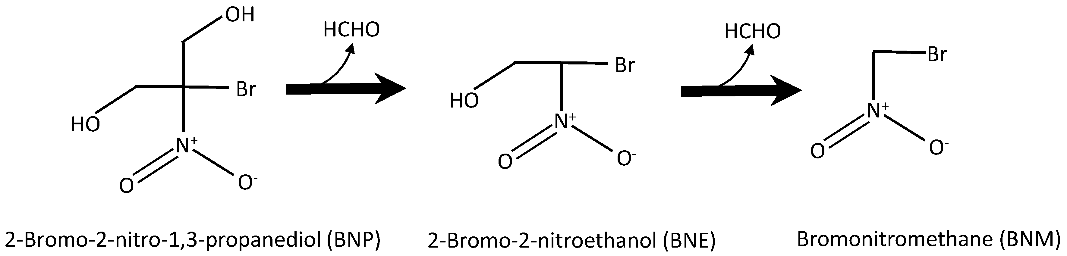
Figure 2.
Algae (Chlorella pyrenoidosa) ecotoxicity for the BNP=>BNE=>BNM degradation pathway as a function of exposure time (data from [87]).
Figure 2.
Algae (Chlorella pyrenoidosa) ecotoxicity for the BNP=>BNE=>BNM degradation pathway as a function of exposure time (data from [87]).

Figure 3.
Soil organic carbon partition coefficient (KOC) and half-life (T1/2) for the BNP=>BNE=>BNM degradation pathway.
Figure 3.
Soil organic carbon partition coefficient (KOC) and half-life (T1/2) for the BNP=>BNE=>BNM degradation pathway.

Figure 4.
Hypothetical example demonstrating organic carbon profile (a), the derived depth-reduction factor (b), the depth-reduction factor applied to the distribution coefficient for three chemicals involved in first-order transformation reactions (c) and the first-order degradation constant for the same three chemicals (d).

Figure 5.
Breakthrough curves of BNP (top), BNE (middle), and BNM (bottom) at 2 and 5 cm soil depth using three parameter combinations: min or low R and max or high half-life (L), mean R and half-life (M), max or high R and min or low half-life (H).
Figure 5.
Breakthrough curves of BNP (top), BNE (middle), and BNM (bottom) at 2 and 5 cm soil depth using three parameter combinations: min or low R and max or high half-life (L), mean R and half-life (M), max or high R and min or low half-life (H).

Figure 6.
Simulated SAR values for Scenario 2 (A), Scenario 3 (B) and Scenario 4 (C). The ANZECC [93] guide value for SAR is 5 for light clay and 20 for sand-sandy loam soil. Note the different scales in the figures.
Figure 6.
Simulated SAR values for Scenario 2 (A), Scenario 3 (B) and Scenario 4 (C). The ANZECC [93] guide value for SAR is 5 for light clay and 20 for sand-sandy loam soil. Note the different scales in the figures.

Figure 7.
Simulated electrical conductivity for Scenario 2 (A), 3 (B) and 4 (C). The ANZECC [93] EC trigger value is 0.65 dS m−1. Note the different scales in the figures.
Figure 7.
Simulated electrical conductivity for Scenario 2 (A), 3 (B) and 4 (C). The ANZECC [93] EC trigger value is 0.65 dS m−1. Note the different scales in the figures.
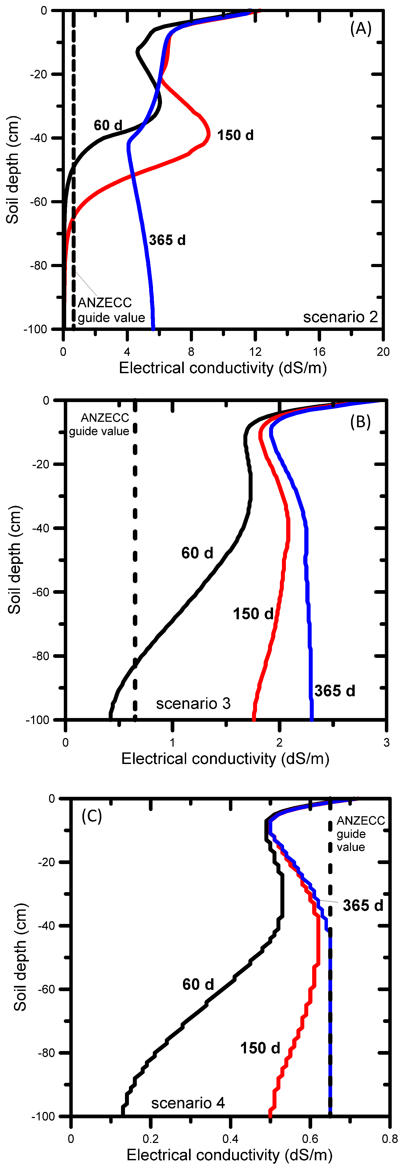
Figure 8.
Cumulative actual evaporation (A), transpiration (B) and drainage (C) rates for Scenario 2 (Sc2), 3 (Sc3), and 4 (Sc4).
Figure 8.
Cumulative actual evaporation (A), transpiration (B) and drainage (C) rates for Scenario 2 (Sc2), 3 (Sc3), and 4 (Sc4).

Figure 9.
Mobile metal ion concentrations for 17 most abundant elements (out of 41). The top and bottom of each bar represents maximum and minimum concentrations, respectively; the horizontal line is the median concentration. (Data from [106]).
Figure 9.
Mobile metal ion concentrations for 17 most abundant elements (out of 41). The top and bottom of each bar represents maximum and minimum concentrations, respectively; the horizontal line is the median concentration. (Data from [106]).
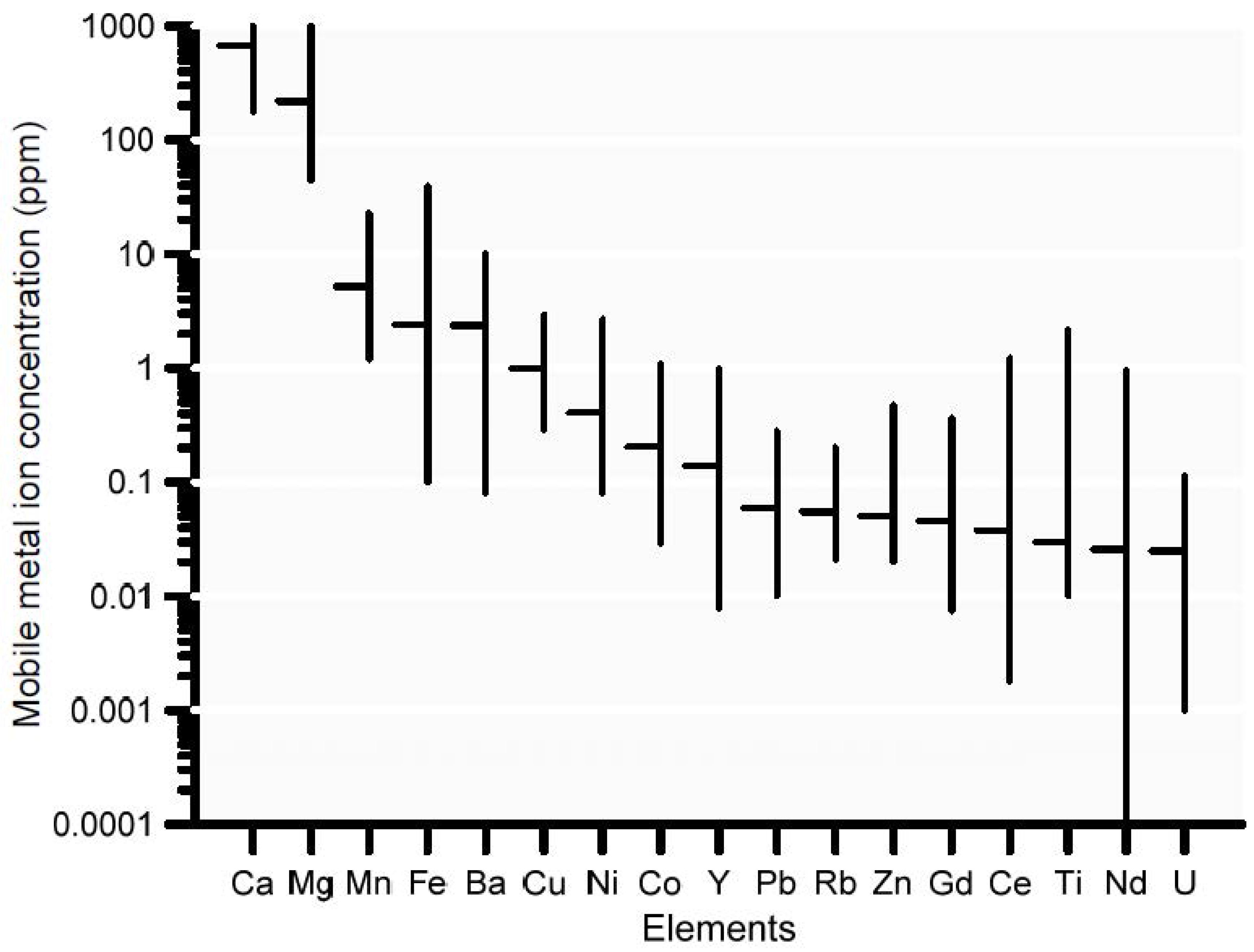
Figure 10.
Simplified chemical composition of produced water used as input solution (only site 3 is reported here).
Figure 10.
Simplified chemical composition of produced water used as input solution (only site 3 is reported here).

Figure 11.
Liquid phase concentrations for lead in a 1-m deep soil profile for 30-y infiltration with produced water (comparison between Scenario 2 [trace metal-free, solid lines] and Scenario 3 [trace-metal containing water [TM, symbols]). Times are as follows: T = 0 y and T = 30 y are the start and end of infiltration with produced water; between T > 30 y and T = 100 y rainwater infiltrated.

Figure 12.
Solid phase concentrations for lead in a 1-m deep soil profile for a 30-y infiltration with produced water (comparison between trace metal-free and trace-metal containing [TM] water). Times are as follows: T = 0 y and T = 30 y are the start and end of infiltration with produced water; between T > 30 y and T = 100 y rainwater infiltrated.

Figure 13.
Depth distribution of the most abundant lead species in the liquid phase at t0 (initial equilibrium condition, left) and t25 (infiltration of produced water, right).
Figure 13.
Depth distribution of the most abundant lead species in the liquid phase at t0 (initial equilibrium condition, left) and t25 (infiltration of produced water, right).

Figure 14.
Lead and chloride bottom solute fluxes as a function of time. Comparison between trace metal-free and trace metal-containing produced water.
Figure 14.
Lead and chloride bottom solute fluxes as a function of time. Comparison between trace metal-free and trace metal-containing produced water.


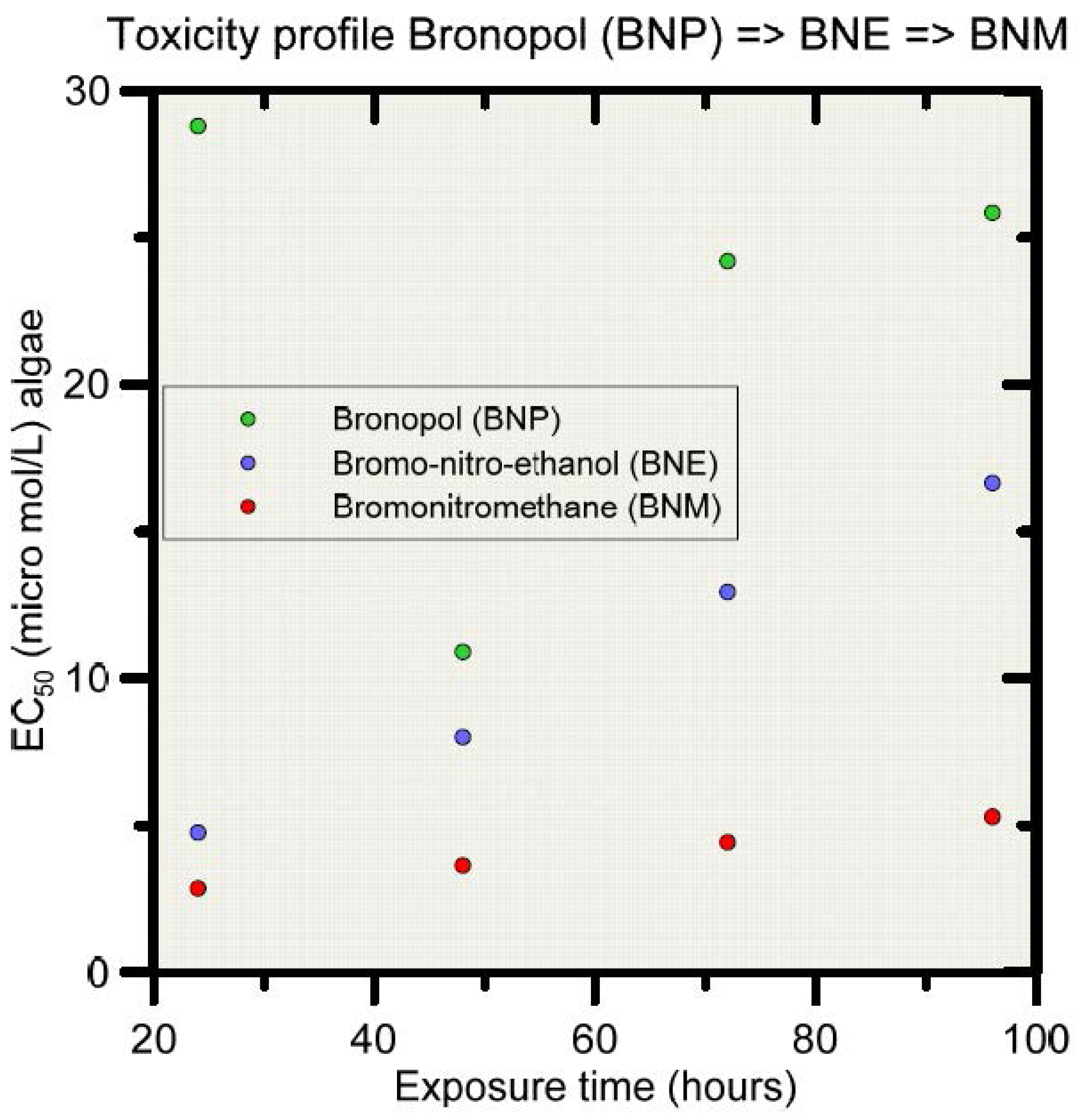
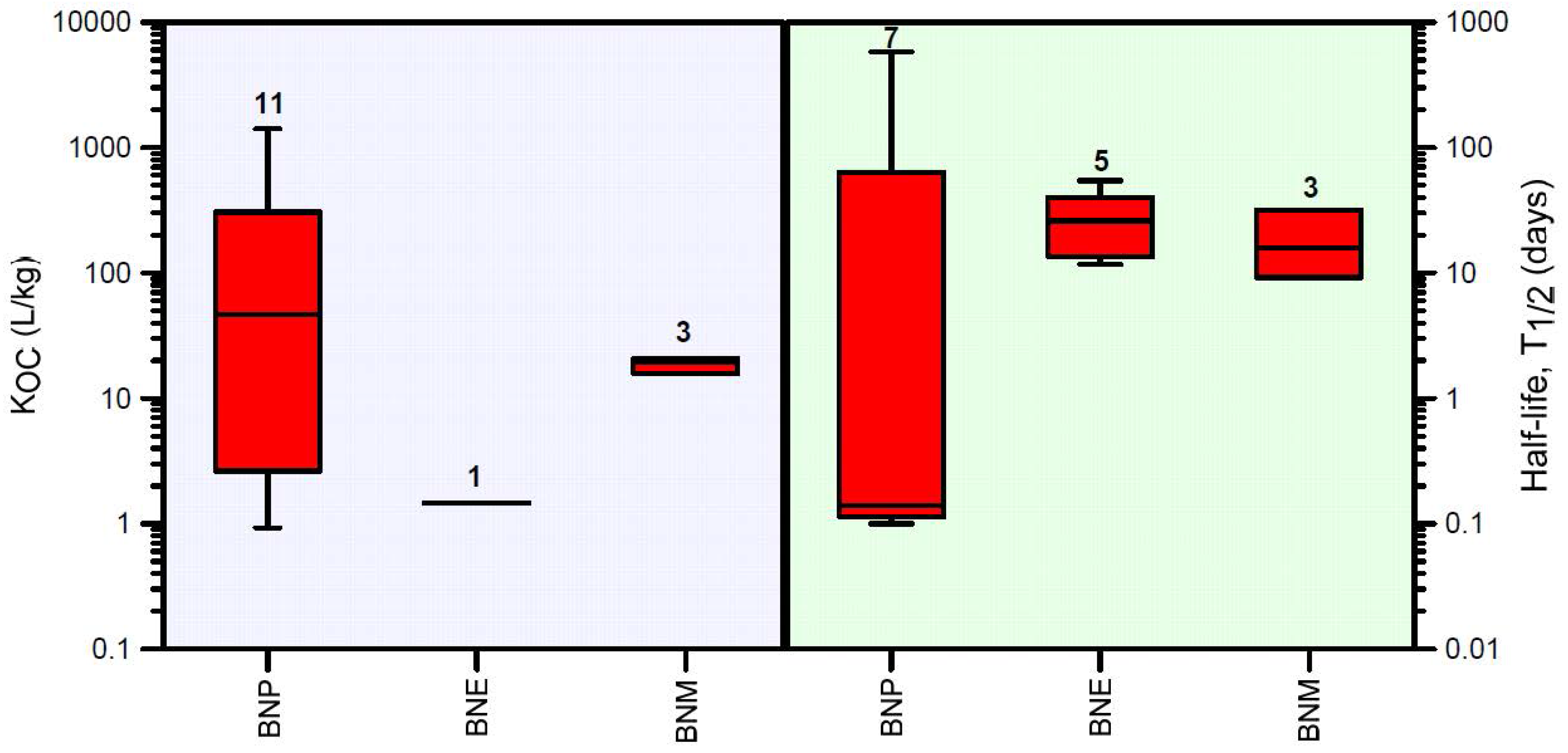
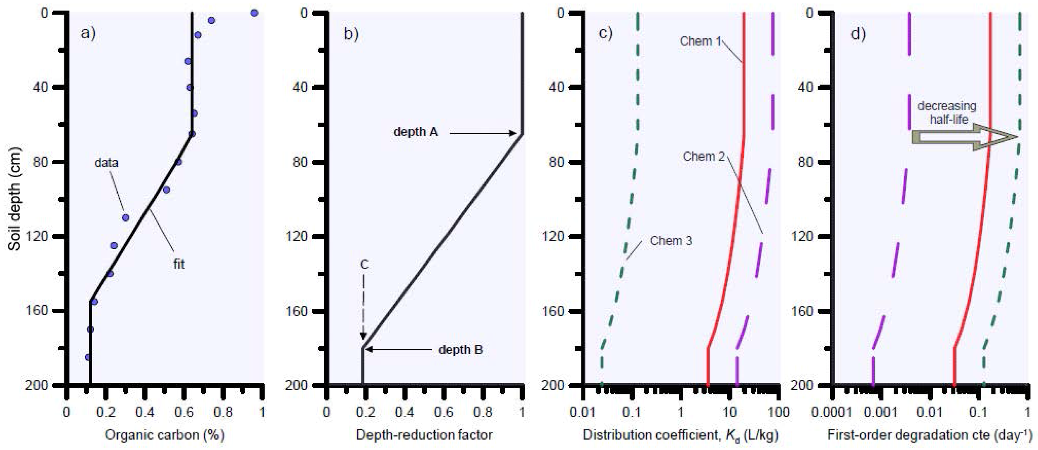
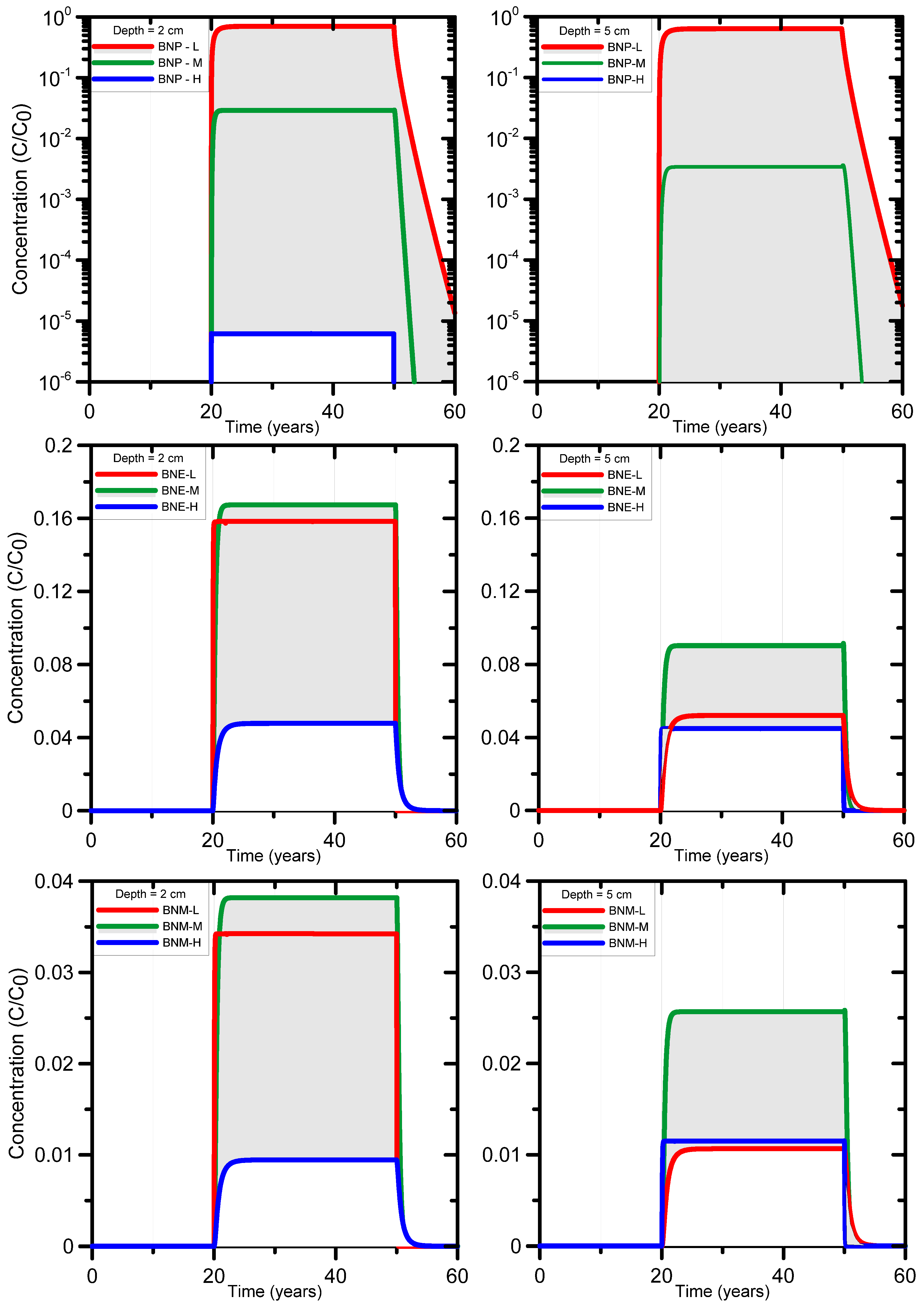
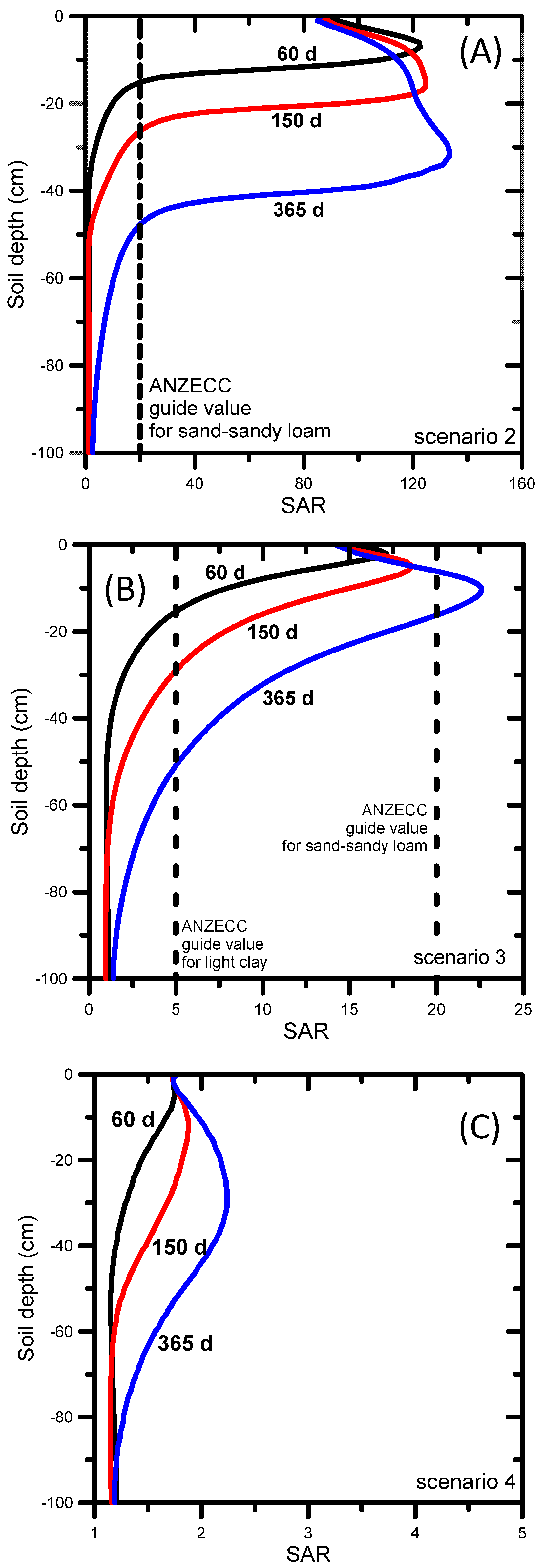
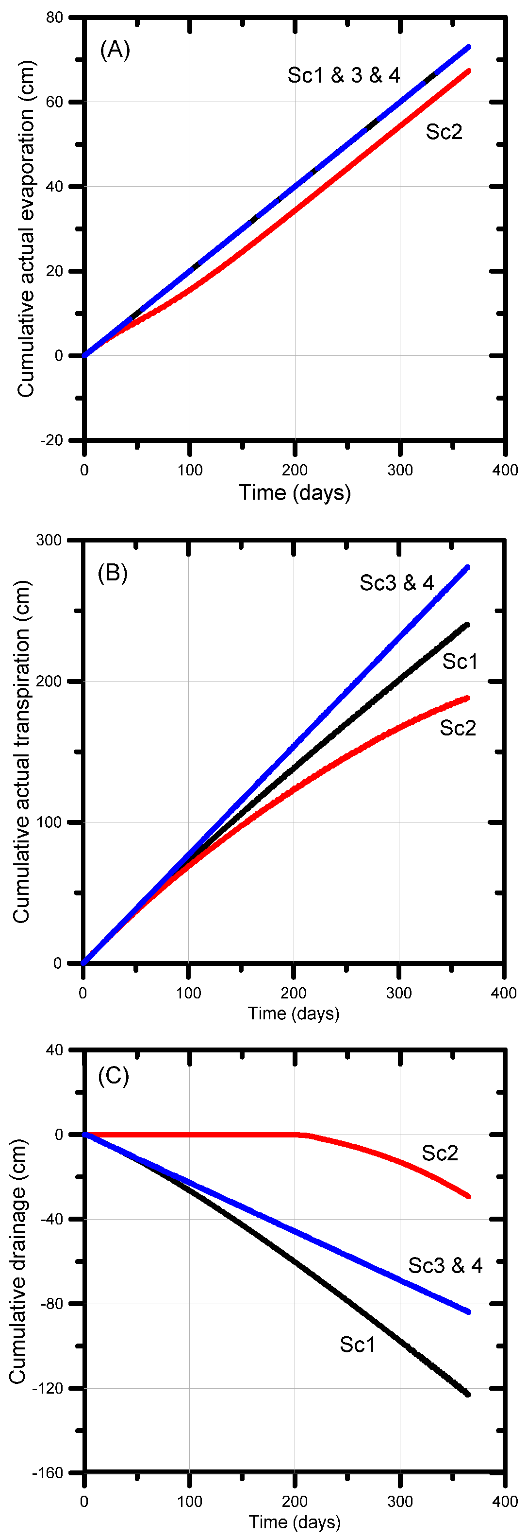
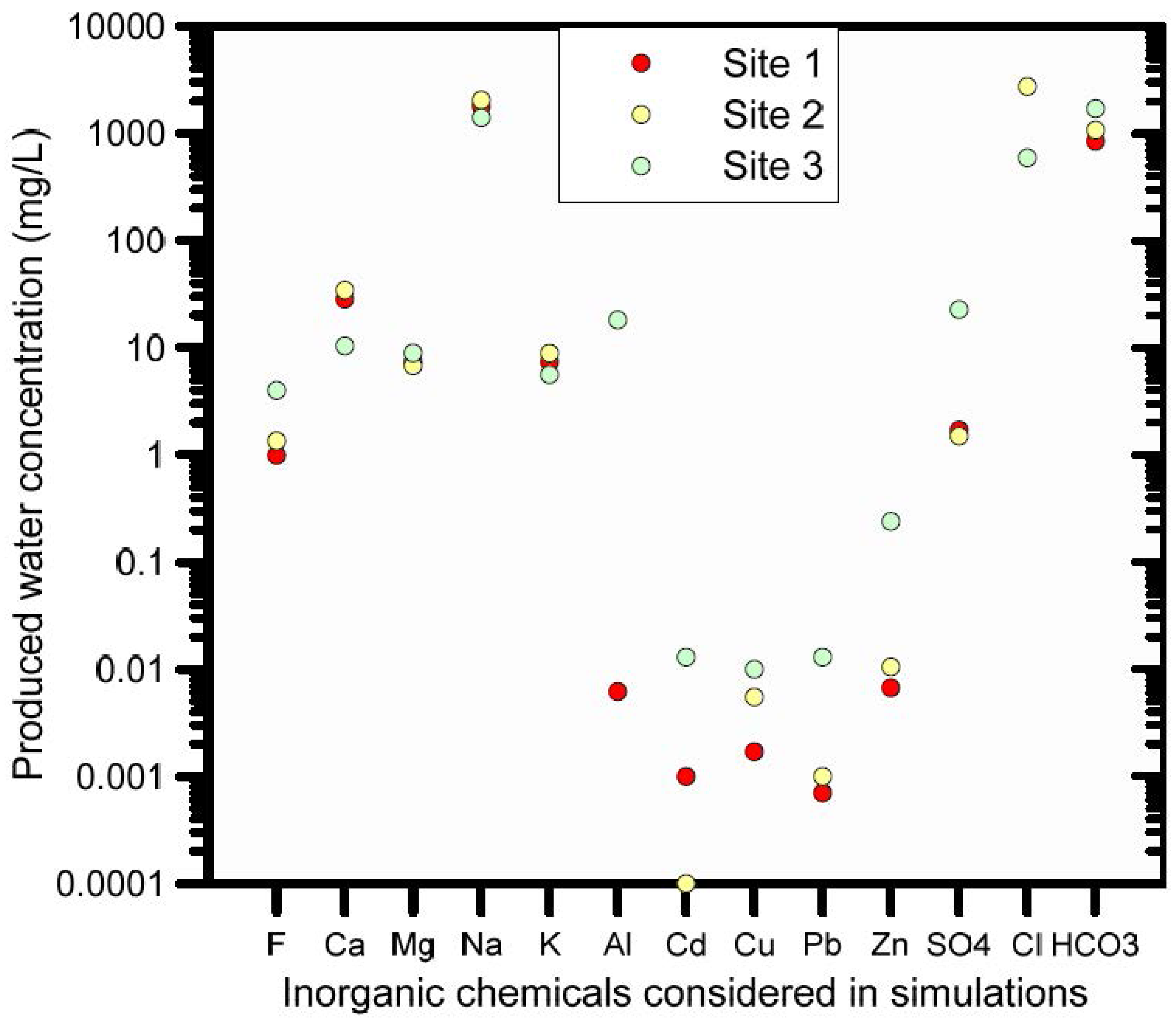
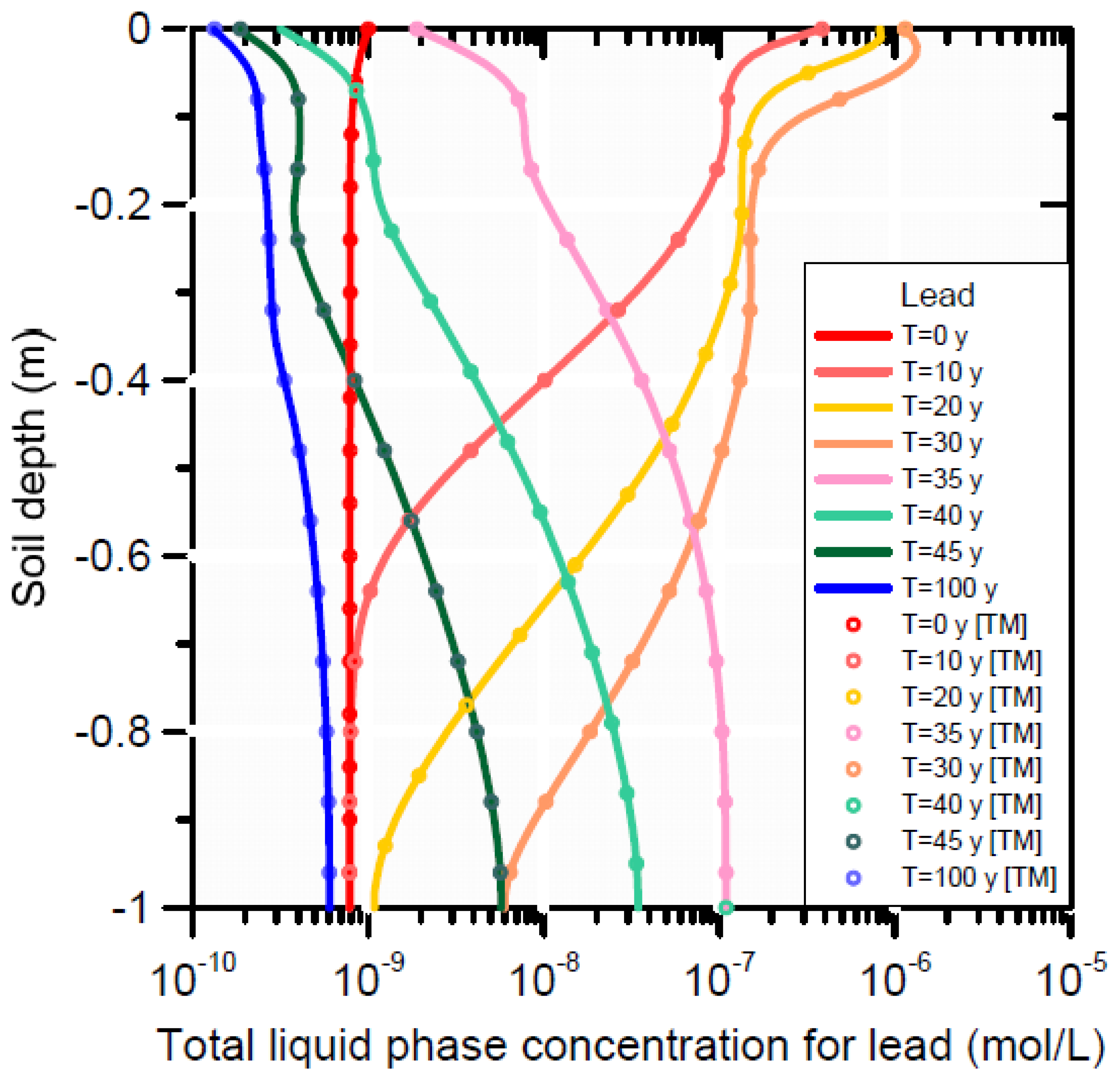
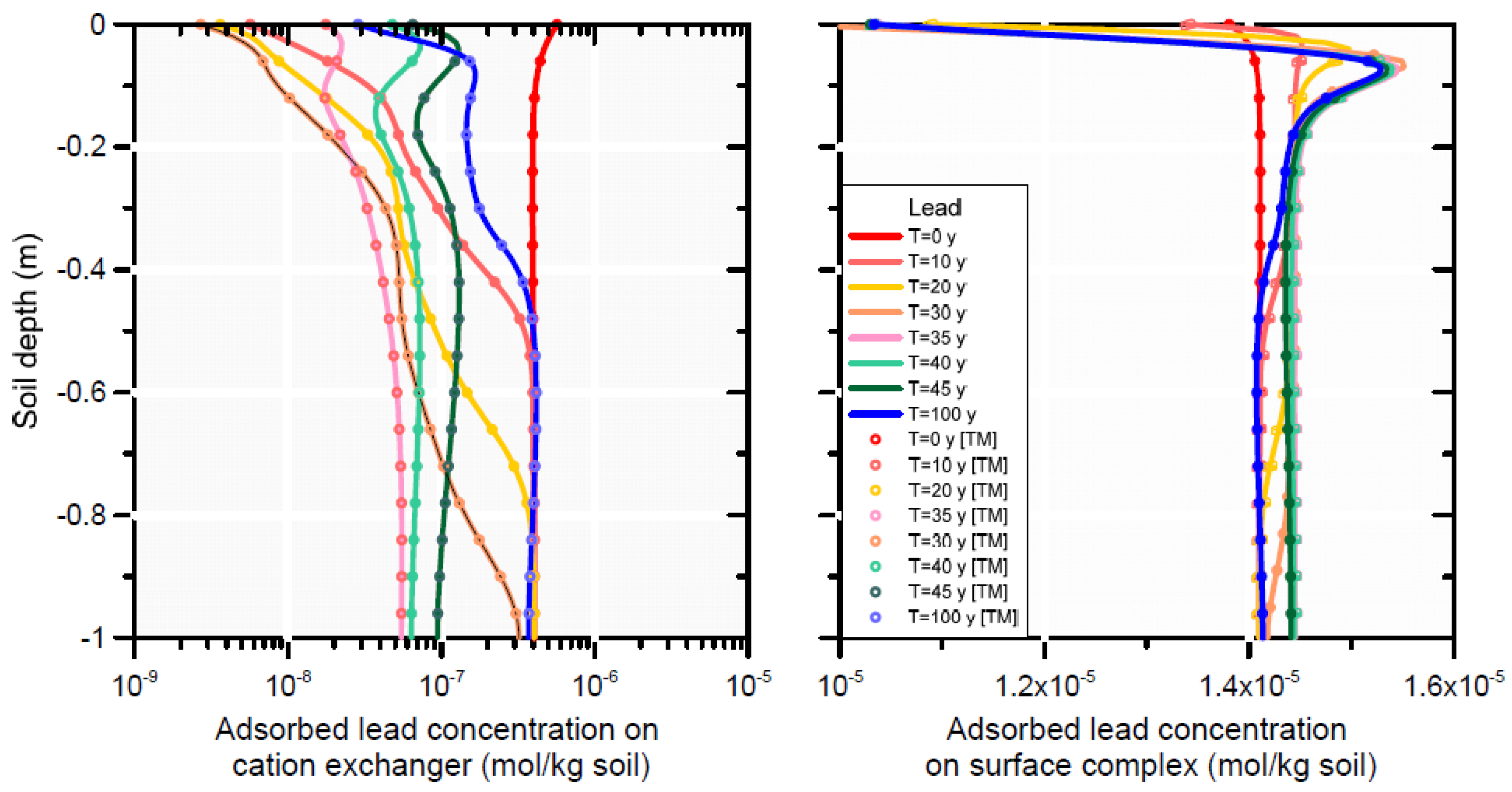
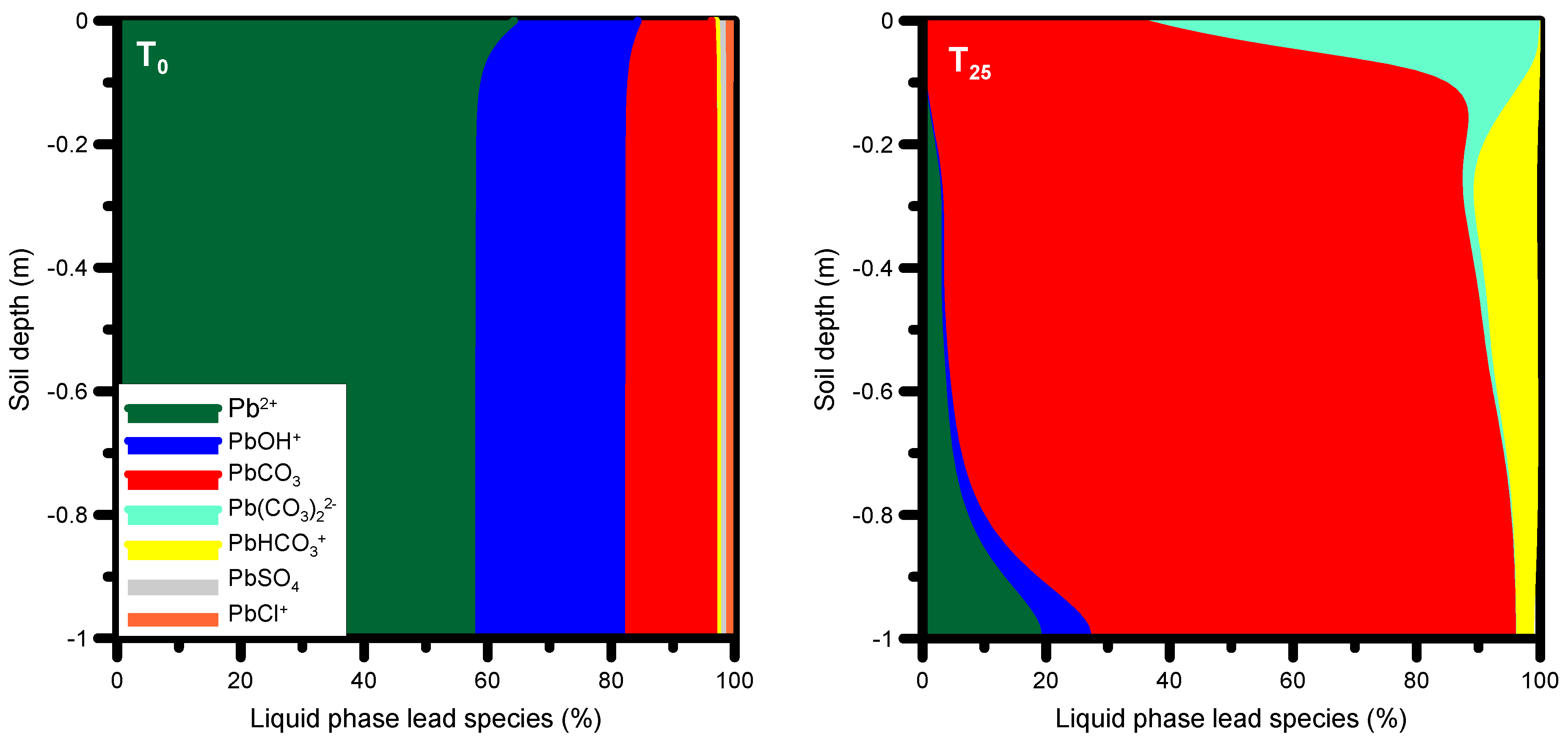
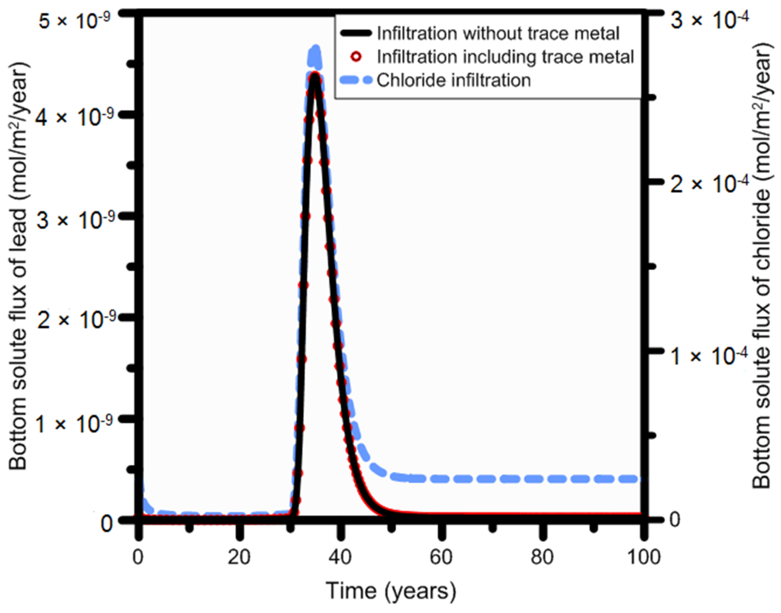
Table 1.
Retardation factors R and aerobic degradation half-lives (T1/2, days) of bronopol and two of its daughter productions. N = number of data (see Supplementary Materials Table S1 for data sources).
Table 1.
Retardation factors R and aerobic degradation half-lives (T1/2, days) of bronopol and two of its daughter productions. N = number of data (see Supplementary Materials Table S1 for data sources).
| Chemical | Mean R | Min R | Max R | N | Mean T1/2 | Min T1/2 | Max T1/2 | N |
|---|---|---|---|---|---|---|---|---|
| Bronopol (BNP) | 187 | 2 | 1170 | 11 | 87 | 0.1 | 548 | 7 |
| 2-bromo-2-nitroethanol (BNE) | 2 | 2 | 2 | 1 | 28 | 11 | 51 | 5 |
| Bromonitromethane (BNM) | 17 | 14 | 18 | 3 | 18 | 8.7 | 30 | 3 |
Table 2.
Composition of untreated, amended, and reverse osmosis (RO) treated produced waters from Australian coal basins. Treated/rain water = a ratio of treated produced water to rain water composition * [99]. SAR = sodium adsorption ratio; ECT = total electrical conductivity.
Table 2.
Composition of untreated, amended, and reverse osmosis (RO) treated produced waters from Australian coal basins. Treated/rain water = a ratio of treated produced water to rain water composition * [99]. SAR = sodium adsorption ratio; ECT = total electrical conductivity.
| Units | Alkalinity | Cl | SO4 | Ca | K | Mg | Na | ECT | SAR |
|---|---|---|---|---|---|---|---|---|---|
| Untreated produced water | |||||||||
| mg L−1 | 1706 | 593 | 22.8 | 10.4 | 5.6 | 8.9 | 1406 | - | - |
| meq L−1 | 41.9 | 16.7 | 0.47 | 0.52 | 0.14 | 0.74 | 61.1 | - | 77 |
| ECi (µS cm−1) @ | 1245 | 1278 | 38 | 31 | 11 | 39 | 3064 | 5705 | - |
| %ECi @ | 21.8 | 22.4 | 0.7 | 0.5 | 0.2 | 0.7 | 53.7 | 100% | - |
| Amended produced water (3:1 ratio surface water:produced water) | |||||||||
| mg L−1 | 183 | 164 | 337 | 10.3 | 34.8 | 6.5 | 184 | - | - |
| meq L−1 | 4.5 | 4.6 | 7.0 | 0.51 | 0.89 | 0.53 | 8.0 | - | 11 |
| ECi (µS cm−1) @ | 134 | 353 | 561 | 31 | 65 | 28 | 401 | 1573 | - |
| %ECi @ | 8.5 | 22.5 | 35.7 | 1.9 | 4.2 | 1.8 | 25.5 | 100% | - |
| RO-Treated produced water | |||||||||
| mg L−1 | 25 | 67 | 1 | 10.33 | 0.43 | 7.6 | 28.7 | - | - |
| meq L−1 | 0.61 | 1.89 | 0.02 | 0.52 | 0.011 | 0.62 | 1.25 | - | 1.6 |
| ECi (µS cm−1) @ | 18.2 | 144.3 | 1.67 | 30.7 | 0.81 | 33 | 62.5 | 291 | - |
| %ECi @ | 6.3 | 49.6 | 0.6 | 10.5 | 0.3 | 11.3 | 21.5 | 100% | - |
| Treated/rain water* | 417 | 103 | 3 | 43 | 4 | 95 | 60 | ||
| Molar conductivity Ʌi for ions as trace concentration in water at 25 °C | |||||||||
| S cm2 mol−1 | 44.5 | 76.35 | 160 | 119 | 73.5 | 106 | 50.1 | ||
@ Calculated with Equation (8).
Table 3.
Cation exchange capacity and surface complexation capacity for 50% cation exchange sites and 50% surface complexation sites (see Supplementary Materials for details). Data from [100].
Table 3.
Cation exchange capacity and surface complexation capacity for 50% cation exchange sites and 50% surface complexation sites (see Supplementary Materials for details). Data from [100].
| Ca2+ | Mg2+ | Na+ | K+ | Total Sorption Capacity | Units |
|---|---|---|---|---|---|
| 0.1745 | 0.0891 | 0.0026 | 0.0129 | 0.279 | [eq kg−1] = [mol(+) kg−1] |
| 0.0875 | 0.0445 | 0.0026 | 0.0129 | 0.147 | [mol kg−1] |
| 0.044 | 0.022 | 0.0013 | 0.0065 | 0.074 | [mol kg−1] 50% |
| Cation exchange capacity | 0.184 | (mole charge dm−3 soil) | |||
| Surface complexation capacity | 0.00826 | (mole charge dm−3 soil) | |||
Table 4.
Aqueous phase species of lead used in the geochemical model (the phreeqcU.dat database used).
Table 4.
Aqueous phase species of lead used in the geochemical model (the phreeqcU.dat database used).
| Aqueous Phase Solution Species | ||
|---|---|---|
| Element | Reaction | logk |
| Pb | Pb2+ + H2O = PbOH++ H+ | −7.71 |
| Pb2+ + 2 H2O = Pb(OH)2 + 2 H+ | −17.12 | |
| Pb2+ + 3 H2O = Pb(OH)3− + 3 H+ | −28.06 | |
| Pb2+ + 4 H2O = Pb(OH)42− + 4 H+ | −39.7 | |
| 2 Pb2+ + H2O = Pb2OH3+ + H+ | −6.36 | |
| Pb2+ + Cl− = PbCl+ | 1.6 | |
| Pb2+ + 2 Cl− = PbCl2 | 1.8 | |
| Pb2+ + 3 Cl− = PbCl3− | 1.7 | |
| Pb2+ + 4 Cl− = PbCl42− | 1.38 | |
| Pb2+ + CO32− = PbCO3 | 7.24 | |
| Pb2+ + 2 CO32−= Pb(CO3)22− | 10.64 | |
| Pb2+ + HCO3− = PbHCO3+ | 2.9 | |
| Pb2+ + SO42−= PbSO4 | 2.75 | |
| Pb2+ + 2 SO42− = Pb(SO4)22− | 3.47 | |
| Pb2+ + NO3− = PbNO3 | 1.17 | |
| Pb2+ + F− = PbF+ | 1.25 | |
| Pb2+ + 2 F− = PbF2 | 2.56 | |
Table 5.
Cation exchange species of the heavy metals included in the geochemical model (the phreeqcU.dat database used).
Table 5.
Cation exchange species of the heavy metals included in the geochemical model (the phreeqcU.dat database used).
| Cation Exchange | ||
|---|---|---|
| Element | Reaction | logk |
| Cd | Cd2+ + 2X− = CdX2 | 0.8 |
| Cu | Cu2+ + 2X− = CuX2 | 0.6 |
| Pb | Pb2+ + 2X− = PbX2 | 1.05 |
| UO2 | UO22+ + 2X− = UO2X2 | 0.8 |
| Zn | Zn2+ + 2X−= ZnX2 | 0.8 |
Table 6.
Surface complexation species of the heavy metals included in the geochemical model (the phreeqcU.dat database used). Note that also H+ and other cation and anions may form surface complexes.
Table 6.
Surface complexation species of the heavy metals included in the geochemical model (the phreeqcU.dat database used). Note that also H+ and other cation and anions may form surface complexes.
| Surface Complexation | ||
|---|---|---|
| Element | Reaction | logk |
| Cd | Hfo_wOH + Cd2+ = Hfo_wOCd++ H+ | −2.91 |
| Cu | Hfo_wOH + Cu2+ = Hfo_wOCu+ + H+ | 0.6 |
| Pb | Hfo_wOH + Pb2+ = Hfo_wOPb+ + H+ | 0.3 |
| UO2 | Hfo_wOH + UO22+ = Hfo_wOUO2+ + H+ | 2.8 |
| Zn | Hfo_wOH + Zn2+ = Hfo_wOZn+ + H+ | −1.99 |
© 2017 by the authors. Licensee MDPI, Basel, Switzerland. This article is an open access article distributed under the terms and conditions of the Creative Commons Attribution (CC BY) license (http://creativecommons.org/licenses/by/4.0/).
Share and Cite
MDPI and ACS Style
Mallants, D.; Šimůnek, J.; Genuchten, M.T.v.; Jacques, D. Simulating the Fate and Transport of Coal Seam Gas Chemicals in Variably-Saturated Soils Using HYDRUS. Water 2017, 9, 385. https://doi.org/10.3390/w9060385
AMA Style
Mallants D, Šimůnek J, Genuchten MTv, Jacques D. Simulating the Fate and Transport of Coal Seam Gas Chemicals in Variably-Saturated Soils Using HYDRUS. Water. 2017; 9(6):385. https://doi.org/10.3390/w9060385
Chicago/Turabian StyleMallants, Dirk, Jirka Šimůnek, Martinus Th. van Genuchten, and Diederik Jacques. 2017. "Simulating the Fate and Transport of Coal Seam Gas Chemicals in Variably-Saturated Soils Using HYDRUS" Water 9, no. 6: 385. https://doi.org/10.3390/w9060385
Note that from the first issue of 2016, this journal uses article numbers instead of page numbers. See further details here.