
Optimising Fuzzy Neural Network Architecture for Dissolved Oxygen Prediction and Risk Analysis


1
Department of Civil Engineering, Lassonde School of Engineering, York University, 4700 Keele St, Toronto, ON M3J 1P3, Canada
2
Department of Mechanical Engineering, University of Victoria, PO Box 1700 STN CSC, Victoria, BC V8P 5C2, Canada
*
Author to whom correspondence should be addressed.
Water 2017, 9(6), 381; https://doi.org/10.3390/w9060381
Submission received: 30 March 2017
/
Revised: 17 May 2017
/
Accepted: 24 May 2017
/
Published: 28 May 2017
(This article belongs to the Special Issue Modeling of Water Systems)
Abstract
:A fuzzy neural network method is proposed to predict minimum daily dissolved oxygen concentration in the Bow River, in Calgary, Canada. Owing to the highly complex and uncertain physical system, a data-driven and fuzzy number based approach is preferred over traditional approaches. The inputs to the model are abiotic factors, namely water temperature and flow rate. An approach to select the optimum architecture of the neural network is proposed. The total uncertainty of the system is captured in the fuzzy numbers weights and biases of the neural network. Model predictions are compared to the traditional, non-fuzzy approach, which shows that the proposed method captures more low DO events. Model output is then used to quantify the risk of low DO for different conditions.
1. Introduction
The dissolved oxygen (DO) concentration of a water body is the most fundamental indicator of overall aquatic ecosystem health [1,2,3,4,5]. Low DO concentrations can increase the risk of adverse effects to the aquatic environment. While the impact of long-term effects is largely unknown, low DO can have immediate and devastating effects on ecosystems [6]. Thus, DO is widely measured and modelled, and the identification and quantification of DO trends in rivers is of interest to water resource managers [7]. However, changes in watershed land-use due to urbanisation, the interaction of numerous factors, over a relatively small area and across different temporal scales means that DO is difficult to predict in urban areas [2,8]. Rapid changes in the urban environment (e.g., land-use changes or major flood events) means that the factors and regimes influencing DO in the riverine environment might also change rapidly.
In Calgary, Alberta, Canada, the Bow River has experienced low DO conditions in recent years. The Bow River is extremely important for the region because it is a source of potable water, and is used for industrial, irrigation, fishing and recreational purposes [9,10]. Thus, maintaining a high water quality standard is extremely important. High sediment and nutrient loads, effluent from three wastewater treatment plants, and stormwater runoff have contributed to reducing the health of the Bow River. The City of Calgary is mandated to meet the requirements of the provincial surface water quality guidelines, which means maintaining DO concentrations above 5 mg/L (one-day minimum), and above 6.5 mg/L (seven-day average) [11]. Thus, in an effort to improve water quality and maintain high DO concentration the City has implemented several strategies to limit loadings such as the Total Loadings Management Plan and the Bow River Phosphorus Management Plan [12].
As part of these plans, the City uses numerical modelling to predict the impact of different strategies within the watershed. However, the physical processes that govern the behaviour of DO in the aquatic environment are quite complex and poorly understood. The physically-based models that are typically used for DO prediction require the parameterisation of a several different variables, which can be unavailable, expensive and time consuming [7,13,14]. In addition to this, physically-based models cannot account for the rapid changes seen in the Bow River watershed, including two major floods in 2005 and 2013, new wastewater treatment plants that have come online, and the relocation of water quality monitoring stations further downstream. These factors highlight the fact that the uncertainty associated with the riverine ecosystem is high. Thus, DO predictions are extremely difficult and beset with uncertainty hindering water resource managers from making objective decisions. Thus, there is a need to create a numerical modelling method that can accurately predict DO concentration whilst accounting for the epistemic uncertainty in the system.
1.1. Data-Driven Models and ANN
The City of Calgary currently uses a physically–based model: the Bow River Water Quality Model [15,16] to predict DO. This model suffers from many of the issues related to complexity and uncertainty that are discussed above. In response to this, recent research [5,14,17,18,19] has shown that data-driven models, particularly those that use abiotic factors as inputs have promising results to predict DO concentration. Examples of the abiotic factors used in these studies are water temperature, nutrient concentration, flow rate and solar radiation. These factors are commonly monitored at a high resolution in many jurisdictions including in Calgary. The advantage of using readily available data in these studies was twofold: first, it makes the system amenable to be modelled using data-driven models; and, second, if a suitable relationship between the abiotic factors and DO can be found, then changing the factors (e.g., increasing the discharge) could increase DO.
Data-driven models are a class of numerical models based on generalized relationships between input and output datasets [20]. These models can characterize a system with limited assumptions and typically have a simple model structure. This means propagating the uncertainty through the model is easier. The use of data-driven models, such as artificial neural networks (ANNs), has been widespread in hydrology [21,22,23] including for DO prediction in rivers. Wen et al. [7] used an ANN to predict DO in a river in China using ion concentration as the predictors. Antanasijević et al. [13] used ANNs to predict DO in a river in Serbia using a Monte Carlo approach to quantify the uncertainty in model predictions and temperature as a predictor. Chang et al. [24] also used ANNs coupled with hydrological factors (precipitation and discharge) to predict DO in a river in Taiwan. Singh et al. [25] used water quality parameters to predict DO and biochemical oxygen demand in a river in India. Other studies (e.g., [26,27]) have used regression methods to predict DO in rivers using water temperature as inputs. In general, these studies have demonstrated that data-driven models can provide a suitable format for predicting DO with lower complexity [13].
ANNs, popular type of data-driven model, are defined as a massively parallel distributed information processing system [7,23]. A commonly used type of ANN is called a Multi-Layer Perceptron (MLP) model which consists of three layers: an input layer, a hidden layer, and an output layer. Each layer consists of a number of neurons that each receives a signal (e.g., the input dataset), and, based on the strength of that signal (quantified by the model coefficients called weights and biases), emits an output. Thus, the final output layer is the synthesis and transformation of all the input signals from the input and hidden layers [28]. The number of neurons in the hidden layer is reflective of the complexity of the system being modelled; more neurons represent a more complex system [23]. The advantage of using ANNs is that complex systems can be modelled by ANNs without an explicit understanding of the physical phenomenon [13,29], making it an ideal candidate for DO prediction in riverine environments. However, recent surveys [30,31] on the state of the use of ANNs in the field indicate that the lack of uncertainty quantification is a major reason for the limited appeal of ANN by water resource managers. Uncertainty in ANN models stem from: (i) the choice of network architecture, e.g., the number of hidden layers, the number of neurons in each hidden layer, and the transfer function between each layer; and the training algorithm used to quantify the weights and biases, including the fraction of data used for training, calibrating and testing; and (ii) the selection of the performance metric used for training which determines the value of the model coefficients. All of these factors can impact the final value of the model coefficients suggesting that a range of values for the weights and biases may be possible for the same dataset [31]. However, most ANN applications have a deterministic structure that does not quantify the uncertainty intervals corresponding to these predictions [32,33]. This means that end-users of these models may have excessive confidence in the forecasted values, and overestimate the applicability of the results [29]. However, as with all numerical models, the appropriate characterisation of uncertainty in a model is essential [34].
1.2. Fuzzy Artificial Neural Networks for Risk Assessment
Alvisi and Franchini [29] introduced a new method to train ANNs which used fuzzy numbers to quantify the total uncertainty in the weights, biases, and output of an ANN. Fuzzy numbers are an extension of fuzzy set theory [35] and express an uncertain or imprecise quantity. Fuzzy numbers are useful for dealing with uncertainties when data are limited or imprecise [36,37,38,39]. In this method, the model coefficients are defined to capture a predefined amount of observed data within different α-cut interval which are used to construct discretised fuzzy numbers. Khan and Valeo [19] further refined this technique by introducing an objective method to select the amount of data to be captured within each interval using the relationship between possibility and probability theory. An advantage of these approaches is that imprecise information (i.e., model output represented through the use of fuzzy numbers) can be effectively used to conduct risk analysis [40]. For example, the model output can be used to determine the risk of occurrence of low DO in the Bow River. However, given the overall preference of the general public and water resource managers for using probabilistic measures (rather than possibilistic or fuzzy measures), there is a need to convert the fuzzy number output of a fuzzy artificial neural network (FNN) to an equivalent probability for communicating risk and uncertainty.
1.3. Objectives
Given the importance of DO concentration as an indicator of overall aquatic ecosystem health, there is a need to accurately model and predict DO in urban riverine environments. In this research, two separate methods are proposed to quantify the uncertainty in an ANN model used to predict DO. First, a transparent algorithm is developed to select the optimum network architecture to maximise model performance. In previous research using this dataset (e.g., [19]), an ad hoc trial and error approach was used in selecting the network architecture. In the current approach, the uncertainty introduced due to the use of data-driven models is carefully considered using the proposed algorithm to find the optimum network architecture. Secondly, a fuzzy number based ANN is implemented to quantify the total uncertainty of the model coefficients and output. Lastly, the application of the developed model is demonstrated by quantifying the risk of low DO in the Bow River using a new method. The results are used to create a tool for water resource managers to assess the risk of conditions that lead to low DO. The importance of the proposed approach is that it: (i) accounts for the complexity of the physical-system by using a data-driven approach; (ii) uses abiotic inputs since they are routinely collected and thus, a large dataset is available; and (iii) minimises the network architecture uncertainty and propagates the total uncertainty in the system through the use of fuzzy numbers. The present research uses crisp inputs as compared to fuzzy inputs in [19] for two practical reasons: (i) in some cases, high resolution data may not be available to construct fuzzy numbers using the algorithm introduced in [19], necessitating the use of observed crisp data (without input uncertainty quantification); and (ii) for the application component of this research, the inputs need to necessarily be crisp numbers in order to create a risk assessment tool for use by water resource managers. In other words, the proposed research will help managers identify the risk of low DO for any number of cases, using pre-selected crisp inputs.
2. Materials and Methods
2.1. Data Collection
The City of Calgary is located in the Bow River Basin (approximately 25,123 km2 in area) in southern Alberta, Canada. The Bow River is 645 km long and averages a 0.4% slope over its length [10]. The headwaters of the river are located at Bow Lake, in the Rocky Mountains, from where it flows south-easterly to Calgary (drainage area of 7870 km2), meeting the Oldman River and eventually draining into Hudson Bay [9,41]. The river is supplied by snowmelt from the Rocky Mountains, rainfall and runoff, and discharge from groundwater. The River has an average annual discharge of 90 m3/s, and an average width and depth of 100 m and 1.5 m, respectively [42].
The City of Calgary samples a variety of water quality parameters along the Bow River to measure the impacts of urbanisation. Real-time water quality monitoring systems are stationed at the upstream (at the Bearspaw reservoir) and downstream (at Highwood) ends of the City (as shown in Figure 1). Comparing water quality data from the stations shows the direct impact of the urban area on the Bow River [18]: concentration at upstream site is generally high throughout the year, with little diurnal variation [5,14,17], whereas the concentration downstream of the City limits is typically lower, and experiences much higher fluctuations. The three wastewater treatment plants (shown in Figure 1) are located upstream of this monitoring site, and are thought to be responsible, along with other impacts of urbanisation, for the degradation of water quality at the site.
For this research, nine years of DO concentration data were collected from the downstream station for the period from 2004 to 2012. From 2004 to 2007, the monitoring station was located at Pine Creek and sampled every 30 min (for 2004 and 2005), and every 15 min (for 2006 and 2007). In 2008 the station was moved to Stier’s Ranch where it remained until 2011, and sampled data every hour (in 2008) and every 15 min from there on. The site was moved further downstream to Highwood in 2012 where it sampled every 15 min. During this period a number of low DO events were observed. The number of days where the observed DO was measured to be below 5 mg/L (the acute guideline) was 25 days in 2004, 1 day in 2005 and 25 days in 2006. The number of days with DO concentration below 6.5 mg/L (the chronic guideline) was more frequent with a total of 184 occurrences: 41, 26, 70, 27, 5 and 15 days in 2004, 2005, 2006, 2007, 2008 and 2009, respectively. A YSI sonde is used to monitor DO and the sonde is not accurate in freezing water [43], thus only data from the ice free period were considered, which is approximately from April to October for most years [19]. Since low DO events usually occur in the summer, the ice-free period dataset contains the dates that are of interest for low DO modelling.
For this research, mean daily water temperature (T) and mean daily flow rate (Q) were selected as the abiotic input parameters for the FNN data-driven model. The reason for selecting these two variables was their use in previous studies in this river basin [5,14,17] which show that these variables are good predictors of DO concentration. The same YSI sonde used to sample DO concentration was used to collect T. The Water Survey of Canada site “Bow River at Calgary (ID: 05BH004 shown in Figure 1) was used to collect Q. These data are collected hourly throughout the year; data where considerable shift corrections are applied (usually due to ice conditions) were removed from the analysis. The mean annual water temperature ranged between 9.23 and 13.2 °C, and the annual mean flow rate was between 75 and 146 m3/s for the selected period.
2.2. ANN and Uncertainty Analysis
For this research, a three layer, feedforward MLP type of ANN was selected to model minimum daily DO (the output) using Q and T as the inputs. Previous studies modelling minimum DO in the Bow River have also used a three-layer MLP feedforward network (see [17]). The type of ANN is extremely popular and thus, forms a reference for the basis of comparing ANN performance [28,29,44]. Two transfer functions were required: one between the input and hidden layer, which was selected as the hyperbolic tangent sigmoid function; and one between the hidden layer and output layer which was a pure linear function (following [7,23,29]). Similarly, the input and output data were pre-processed before training the network: the data were normalised so that all input and output data fell within the interval [−1, +1]. Model coefficients were calculated by minimising the mean squared error (MSE) between the modelled output and observed data (minimum DO). The Levenberg–Marquardt algorithm (LMA) was used as the training algorithm [45]. In LMA the error between the output and target is back-propagated through the model using a gradient method where the weights and biases are adjusted in the direction of maximum error reduction. To prevent over-fitting an early-stopping procedure is used [31,45] where the data are first split into three subsets (training, validation and testing). The training is terminated when the error on the validation subset increases from the previous iteration.
2.2.1. Network Architecture
Two remaining factors relating to ANN architecture that need to be identified are: the number of neurons in the hidden layer (nH), and the amount of data used for training, validation and testing (known as data-division) for the early-stopping procedure described above. There is no consistent method used in the literature for each of these factors [30,46,47]. Typically, an ad hoc, or trial-and-error method is used to select the number of neurons [17,23,29,31]. The number of neurons selected must balance the complexity and generalisation of the final model; too many neurons increase the complexity and hence the processing speed, while reducing the transparency of the model. Not enough neurons risk reducing model performance and forgoing the ability of modelling non-linear systems. Similarly, the issue of data-division, which can have significant impacts on final model structure, is also predominantly conducted in an ad hoc and trial-and-error basis [31]. Generally speaking, two broad methods are available: In the first, each subset should have data that are statistically similar, including similar patterns or trends. Conversely, a method can be selected where each subset is based on some physical property, such as grouping the subsets chronologically.
In this research, we propose a coupled method to select the optimum nH and data-division for the ANN model described. The smallest number of neurons and the least amount of data for training is targeted. The first is to reduce computational effort. The second is to prevent the risk of over-fitting to the training data, and to have a larger dataset for testing for more robust statistical inference of that dataset.
First, the dataset is randomly split into a 50%:25%:25% ratio for training, validation and testing, respectively. For each subset, data are randomly sampled to group into each subset. Then, the network is trained using 1 to 20 neurons. This process is repeated 100 times to account for the different selection of randomly sampled data in each subset. This is because the random initialisation of the ANN can cause variability in overall model performance [44]. Thus, each iteration is different than the previous. The MSE for each test dataset is then calculated and compared, as well as the number of epochs for each model is measured. Epochs are the number of times each weight and bias is modified in the optimisation algorithm. The configuration that leads to the lowest MSE and the lowest number of epochs was collected. This process is then repeated by sequentially increasing the amount of data used for training (and thus, reducing the amount of data equally partitioned for validation and testing) by increments of 0.5% from 50% to 75%, conducting each iteration of this change 100 times.
Using this process, the cases where the highest performance was measured can be listed, and the best combination (i.e., nH and amount of training data) can be objectively selected. In doing so, both the processing time (i.e., the number of epochs, the amount of training data and nH) and the complexity (nH) of the system is accounted for in the final model architecture.
2.2.2. Network Coefficients
In the fuzzy ANN method developed by Alvisi and Franchini [29], the standard MLP model is modified to predict an interval rather than a single value for the weights, biases and outputs, corresponding to an α-cut interval (the lower and upper limits of a fuzzy set at a defined membership level α). This is repeated for several α-cut levels between 0 and 1 thus, building a discretised fuzzy number. The constraints are such that to find the upper and lower limits of each weight and bias to minimize the width of the predicted interval while capturing a predefined amount of data within each interval. Khan and Valeo [19] refined this method by utilising the relationship between possibility theory and probability theory, known as probability-possibility transformations (see [48,49,50,51,52]) for details). Khan and Valeo [19] adopted the transformation proposed by Dubois et al. [53], where the possibility is viewed as the upper envelope of the family of probability measures [50,54,55,56]. The same procedure is used in the present research to train the fuzzy ANN using deterministic inputs to construct fuzzy number coefficients (weights and biases) and outputs. Five intervals were selected corresponding to a membership level of 0, 0.2, 0.4, 0.6, and 0.8, with the deterministic result processed equivalent to a membership of 1.
This FNN optimisation algorithm was implemented in MATLAB (version 2015a). The crisp results of the ANN (at a membership level, μ = 1) were conducted using the built-in MATLAB Neural Network Toolbox. Subsequent optimisation for the other intervals was conducted using a two-step approach: first the Shuffled Complex Evolution algorithm (commonly known as SCE-UA, [57]) was used to find an initial solution to the minimisation problem. Then, further refinement of the solution was conducted using the built-in MATLAB minimisation function fmincon.
2.3. Risk Analysis
A major component of this research is to be able to use a trained fuzzy ANN model to predict the risk of low DO using abiotic inputs. However, communicating uncertainty, which can be done in a number of different ways, is an important, yet difficult task [58]. In this research defuzzification is used to convert the possibility of low DO (i.e., predicted minimum fuzzy DO to be below a given threshold) to a probability measure. The transformation is given as follows (following Khan and Valeo [18,19,42]): for any x in the support (the α-cut interval at μ = 0) of a fuzzy number [a, b], we have the corresponding μ(x) and the paired value x' which also shares the same membership level. The value μ(x) is the sum of the cumulative probability distribution between [a, x] and [x', b], labelled AL and AR, respectively:
where AL represents the cumulative probability between a and x which is assumed to equal the probability P(X < x), since the fuzzy number defines any values to less than a to be impossible (i.e., μ = 0). Given the fact that the fuzzy number is not symmetrical, the lengths of the two intervals [a, x] and [x', b] can be used to establish a relationship between AL and AR. Then, AL can be estimated as:
μ(x) = AL + AR,
AL = P(X < x) = μ(x)/{1 + [(b − x')/(x − a)]}.
Thus, Equation (2), gives the probability that the predicted minimum DO for a given day is below the threshold value x. For example, if the lowest acceptable DO concentration of 5 mg/L [11] is selected as this threshold, then this transformation can be used to calculate the probability that daily minimum DO is below 5 mg/L. Similarly, the same principle can be used to map out all combinations of input values that lead to a risk of low DO (i.e., below 5 mg/L or any other threshold value). Once this is mapped out, combinations that lead to a major risk of low DO can be identified by water resource managers.
The overall objective is to provide a simple tool to quantify the risk of low DO under selected T and Q conditions. For this research, the calibrated FNN model was used to predict minimum DO for various combinations of Q and T: where Q ranged between 40 m3/s and 220 m3/s (at 2 m3/s intervals), and T ranged between 0 and 25 °C (at 0.2 °C intervals). For each prediction, the risk of low DO to be below either 5, 6.5 or 9.5 mg/L threshold was calculated using the previously described defuzzification technique. These intervals of Q and T were selected to reflect typical conditions in the Bow River. The thresholds correspond to the minimum acceptable DO concentration for the protection of aquatic life for 1-day (at 5 mg/L) [11], and for the protection of aquatic life in cold, freshwater for early-life stages (at 9.5 mg/L) and other-life stages (6.5 mg/L) [3].
3. Results and Discussion
3.1. Network Architecture
A three-layer, feedforward MLP network architecture was selected with 2 input variables and 1 output variable. A coupled method was used to determine the optimum nH and the percentage of data for each of the training, validation and testing subsets. Sample results of the proposed method are shown in Figure 2. Figure 2a shows the mean MSE (solid black line) of the test dataset for the initial 50%:25%:25% data-division scenario, with nH varying between 1 and 20 neurons. This simulation was repeated 100 times to account for the random selection of data and the upper and lower limits of MSE for each of these simulations are shown in grey. This figure demonstrates that the number of neurons did not have a noticeable impact on the MSE for this configuration. The most significant outcome of this process is that the variability (the difference between the upper and lower limits) of the performance seems to decrease after nH = 6 and increases again after nH = 12, with the lowest MSE at nH = 10. This result has two important implications: first, increasing the model complexity results in limited improvement of model performance, suggesting that a simpler model structure may be more suitable to describe the system. Second, the variability in performance indicates that the initial selection of data in each training subset can highly influence the performance of the test dataset, especially at the lower (i.e., nH < 6) and higher (i.e., nH > 12) ends of the spectrum of the proposed number of neurons. This suggests that an optimum selection of hidden neurons lies within this range (6 < nH < 12).
Figure 2b shows the change in the mean (solid black line) and the variability (in grey) of the number of epochs needed to train the network for the initial data-division scenario, as nH increases from 1 to 20. While the mean value does not show a notable change, the variability of the time needed for training (i.e., the number of epochs) drastically decreases as nH increases from 1 to 5. This means that a simpler model structure may require more time to train, and the performance of these simpler architectures (nH = 1 to 5) is more variable. This is likely because the initial dataset selection has a higher impact on the final model performance for less complex models. The lowest number of mean epochs for this analysis occurred at nH = 19, with 26 epochs. However, note that the variability of MSE at nH = 19 (in Figure 2a) is high, and that nH = 19 falls outside the range 6 < nH < 12, identified above.
The impact of changing the amount of data used for training, validation and testing on the model performance (MSE) was generally inconclusive as the amount of data used for training was increased from 50% to 75% at 0.5% intervals. Figure 2c shows sample results for the nH = 10 scenario, which was the best performing scenario, i.e., had the lowest mean MSE for each data-division scenarios when compared to other nH values. However, the subplot illustrates that the MSE for the test dataset does not show a major trend as the amount of data for training is increased from the initial 50%. This means that for this scenario (nH = 10) increasing the amount of data used for training has minimal impact on model performance, indicating that using the least amount of data for training (and thus having a higher fraction available for validating and testing) would be ideal. Note that the mean MSE values were generally higher for all data-division scenarios when the selected nH was between 1 and 5 (follow the example shown in Figure 2a).
The number of epochs needed for training the network at different data-division scenarios was inconclusive. Figure 2d shows sample results for the nH = 10 case, which demonstrates that the mean and the variability of the number of epochs does not demonstrate a clear trend, as the amount of data used for training is increased. The significance of this analysis is that the amount of computational effort (or time) does not necessarily decrease as a larger fraction of data is used for training. Given this result, the least amount of training data (50%) is the preferred choice for the number of neurons that result in the lowest MSE, which is nH = 10 as described above. For the nH = 10 case, the overall mean number of epochs for each data-division scenario is low ranging between 24 and 40 epochs.
Based on these results, nH = 10 with a 50%:25%:25% data-division was selected as the optimum architecture for this research. The fact that the mean and the variability of MSE was the lowest at nH = 10 makes it a preferred option over the nH = 19 case, which as a lower number of mean epochs but had higher variability in MSE. In other words, higher model performance was selected over model training speed (mean epochs at nH = 10 ranged between 9 and 122 for the 50%:25%:25% data-division scenario). Secondly no significant trend was seen as the amount of data used for training, validation and testing was altered, however lower MSE values were seen at nH = 10 compared to other at nH values. Thus, the option that guarantees the largest amount of independent data for validation and training is preferred. Given the fact that the mean MSE for the testing dataset does not show a significant change as the per cent of training data is increased from 50% to 75%, the initial 50%:25%:25% division is maintained as the final selection.
The overall outcome of this component of this research was that that instead of using the typical trial-and-error based approach to selecting neural network architecture parameters, the proposed method can provide objective results. Specifically, systematically exploring different numbers of hidden layers and fraction of training data can help select a model with the highest performance, whilst accounting for the randomness in data selection. Once these neural network architecture parameters were identified, subsequent training of the FNN was completed. The results of the training and optimisation are presented in the next section.
3.2. Network Coefficients
First, the network was trained at μ = 1 using the network structure outlined in the previous section. The crisp, abiotic inputs (Q and T) were used to estimate the values of each weight and bias in the network. This amounted to 20 weights (10 for each input) and 10 biases between the input and hidden layer, and 10 weights and 1 bias in the final layer. The MSE and the Nash–Sutcliffe model efficiency coefficient (NSE; [59]) for the training, validation and testing scenarios for the μ = 1 case are shown in Table 1 below.
The MSE for each dataset is low, approximately between 10% and 18% of the mean annual minimum DO seen in the Bow River for the study period. The NSE values are greater than 0.5 for each subset, which is higher than NSE values for most water quality parameters (when modelled daily) reported in the literature [60] and is considered “satisfactory” using the ranking system proposed by Moriasi et al. [60]. These two model performance metrics highlight that predicting minimum DO using abiotic inputs and a data-driven approach is an effective technique. Note that compared to results reported in [19], the present modelling approach (with the optimised network architecture) produces similar performance metrics (i.e., “satisfactory”). However, note that in the present case the network architecture selection is selected using an explicit and transparent algorithm, rather than in an ad hoc manner as in [19]. While both methods use the same dataset, the network architecture (number of neurons) is different for both methods, resulting in minor discrepancies between the model performance metrics. Additionally, some results in [19] are derived from fuzzy inputs rather than crisp inputs (as is the case in the present work). Additional advantages of the proposed approach are seen when the fuzzy component of the results are analysed.
Once the crisp network was trained, a top down approach was taken to train the remaining intervals, starting at μ = 0.8 where 20% of the observations should be captured within the corresponding predicted output interval, and continuing to μ = 0 where 99.5% of the observations should be captured within the predicted output intervals. Each set of optimisation (both the SCE-UA and fmincon algorithms) for each of the five remaining membership levels (μ = 0, 0.2, 0.4, 0.6 and 0.8) took approximately 2 h using a 2.40 GHz Intel® Xeon microprocessor (with 4 GB RAM). The results of this optimisation are summarised in Table 2, which shows the amount of data captured within the resulting α-cut intervals after each optimisation.
For the training dataset, the coupled algorithm was able to capture the exact amount of data it was required to. Similar results can be seen for the validation and testing datasets, where the amount of data captured are close to the constraints posed. For the two independent datasets, the amount of coverage decreases (i.e., lower performance) as the membership level increases, which is unavoidable when the width of the uncertainty bands decrease. Similar results were seen for the testing dataset in [29]. These results are similar to those published in [19] for both the fuzzy and crisp input case, with the only marked differences are: at the µ = 0.4 level where the present model captures a lower percentage of data than the crisp case in the previous method; and at the µ = 0.2 and 0.8 levels where the present model captures data closer to the assigned constraints as compared to the fuzzy inputs case in [19].
The result of this optimisation was the calibrated values of the fuzzy weights and biases; sample membership functions for four weights and biases are shown in Figure 3. The figure illustrates that the shapes of all membership functions were convex, a consequence of the top-down calibration approach, where the interval at lower membership levels is constrained to include the entire interval at higher membership levels. In other words, since lower membership levels include a higher amount of data, the corresponding interval to that level is wider than at higher membership levels. Furthermore, since the crisp network was used at μ = 1, there is at least one element in each fuzzy number with μ = 1, meaning that each weight and bias is a normal fuzzy set.
The membership functions of the weights and biases are assumed to be piecewise linear following the assumption made in [5,14,19,29]. This means that enough α-cut levels need to be selected to completely define the shape of the membership functions. In this research six levels were selected to equally span, and to give a full spectrum of possibilities, between 0 and 1. Overall, the results of the weights and biases in the figure demonstrate that indeed enough levels were selected to define the shape of the membership function. If a smaller number of levels were selected, e.g., two levels, one at μ = 0 and one at μ = 1, the fuzzy number collapses to a triangular fuzzy number. This type of fuzzy number does not provide a full description of the uncertainty and how it changes in relation to the membership level. Thus, intermediate intervals are necessary and the results demonstrate that the functions are in fact not triangular shaped functions and not necessarily symmetric about the modal value (at μ = 1). A consequence of this is that the decrease in size of the intervals does not follow a linear relationship with the membership level. Similarly, a higher number of intervals than the six selected for this research could be used, e.g., 100 intervals, equally spaced between 0 and 1. The risk in selecting many intervals is that as the membership level increases (closer to 1) the intervals become narrower as a consequence of convexity. This will result in numerous closely spaced intervals, with essentially equal upper and lower bounds, making the extra information redundant. This is demonstrated in the sample membership functions for WIH = 10 in Figure 3, where increasing the number of membership levels between 0.4 and 1.0 would not improve the shape or description of the membership function. This is because the existing intervals are already quite narrow. Defining more uncertainty bands between the existing levels would not add more detail but would merely replicate the information already calculated.
Table 2 and Figure 3 demonstrate the overall success of the proposed approach to calibrate an FNN model. Whereas in many fuzzy set applications the membership function is not defined or selected based on a consistent, transparent or objective method [30,46,47], or is selected arbitrarily (as noted in [29]), the method proposed in this research is based on possibility theory and provides an objective method to create membership functions. The results of the process show that the method is capable in creating fuzzy number weights and biases that are convex and normal, and capture the required percentage of data within each interval.
Figure 4 shows the results of observed versus crisp predictions (black dots) and fuzzy predictions (black line) of minimum DO at the membership level μ = 0 for the three different data subsets. The figure illustrates that nearly all (i.e., ~99.5%) of the observations fall within the α-cut interval defined at μ = 0 since the black dots are enveloped by the grey high-low lines of the fuzzy interval. The figure also demonstrates the advantage of the FNN over a simple ANN: while some of the crisp predictions veer away from the 1:1 line (especially at low DO, defined to be less than 6.5 mg/L here), nearly-all (i.e., ~99.5%) of the fuzzy predictions intersect the 1:1 line. This also illustrates that the NSE values reported in Table 1 (which were calculated for the crisp case at μ = 1 only) are not representative of the NSE values of the fuzzy number predictions, and that there is a need to develop an equivalent performance metric when comparing crisp observations to fuzzy number predictions.
Lastly, the figure demonstrates the superiority of the FNN to be able to predict more of the low DO events compared to the crisp method. The low DO range (at DO = 6.5 mg/L) is highlighted in Figure 4, and it is apparent that within this window both models tend to over predict minimum DO as they fall above the 1:1 line. However, the fuzzy intervals (grey lines) predicted by the FNN intersect the 1:1 line for the majority of low DO events, and hence predict some possibility (even if it is a low probability) at any μ of the low DO events, whereas the crisp do not predict any possibility at all. Thus, generally speaking the ability of the FNN to capture 99.5% of the data within its predicted intervals guarantees that most of the low DO events are successfully predicted. This is a major improvement over conventional methods used to predict low DO. Comparing Figure 4 to similar results reported in [19] demonstrate that the proposed approach in the present research has improved model performance. Specifically, the predicted intervals at µ = 0 are centred on the output rather than skewed. An outcome of this is that there are a lower number of “false alarms” (i.e., predicting low DO event when observed DO was not low) compared to [19]. This is discussed in more detail below. This suggests that by using an optimised algorithm for the network, low DO prediction is improved, at the expense of a predicting high DO events (i.e., the upper limit of the predicted intervals). However, high DO values are of less interest and importance to most operators. Figure 5 and Figure 6 show trend plots of observed minimum DO and predicted fuzzy minimum DO for the years 2004, 2006, 2007 and 2010. These particular years were selected due to the high number of low DO occurrences in each year, and, thus, are intended to highlight the utility of the proposed method. Note that, for each year shown, approximately 50% of the data constitute training data, while the other 50% constitute a combination of validation and testing data. However, for clarity, this difference is not explicitly shown in these figures.
The most number of days where minimum daily DO was below the 5 mg/L guideline was observed in 2004 and 2006, with 25 days in each year. The year 2007 had the third most (after 2006 and 2004, respectively) number of days below the 6.5 mg/L guideline, with 27 days. Lastly, 2010 had the second most number of days below the 9.5 mg/L guideline with 180 days (after 2007 which had 182) below the guideline. Thus, these four years collectively represent the years with the lowest minimum daily DO during the study period. It is noteworthy that even though minimum DO was observed to be below 5 mg/L on several occasions in 2004 and 2006, the DO was below on 9.5 mg/L only 107 and 164 days, respectively, for these years. In contrast, in 2007 and 2010, no observations below 5 mg/L were seen, however 182 and 180 days, respectively, below the 9.5 mg/L were seen for those years. This indicates that even if no observations of DO < 5 mg/L are seen, it is not a good indicator of a healthy ecosystem, since the overall mean DO of the year might be low (e.g., a majority of days below the 9.5 mg/L). The implication of this is that only using one guideline is not a good indicator of overall aquatic ecosystem health.
In Figure 5 and Figure 6, the predicted minimum DO at equivalent membership levels (e.g., 0L or 0R) at different times steps are joined together creating bands representative of the predicted fuzzy numbers calculated at each time step. Note that the superscripts L and R define the lower bound and upper bounds of the interval at a membership level of 0, respectively. In doing so, it is apparent that all the observed values fall within the μ = 0 interval for the years 2006, 2007 and 2010, and nearly all observations in 2004. This difference in 2004 is because the per cent of data included within the μ = 0 interval was selected to be 99.5% rather than 100% to prevent over-fitting; the optimisation algorithm was designed to eliminate the outliers first to minimise the predicted interval. The low DO values in 2004 are the lowest of the study period, and thus are not captured by the FNN.
The width of each band corresponds to the amount of uncertainty associated with each membership level, for example, the bands are the widest at μ = 0, meaning the results have the most vagueness associated with it. Narrower band are seen as the membership level increases until μ = 1, which gives crisp results. This reflects the decrease in vagueness, increase in credibility, or less uncertainty of the predicted value. In each of the years shown, note that the observations fall closer to the higher credibility bands, except for some of the low DO events. This means that the low DO events are mostly captured with less certainty or credibility (typically between the 0L and 0.2L levels) compared to the higher DO events. However, it should be noted that compared to a crisp ANN, the proposed method provides some possibility of low DO, whereas the former only predicts a crisp result without a possibility of low DO. Thus, the ability to capture the full array of minimum DO within different intervals is an advantaged of the proposed method over existing methods.
Results from 2004 show that minimum DO decreases rapidly starting in late June and continuing until late July, followed by a few days of missing data and near-zero measurements, before increasing to higher DO concentration. Details of this trend are shown in Figure 7. The reason for this rapid decrease is unclear and may be an issue with the monitoring device. However, it demonstrates that the efficacy of data-driven methods is dependent on the quality of the data. One of the advantages of the proposed method is that while it is able to capture nearly all of the observations (including outliers) within the least certainty band (at μ = 0), other observations are mostly captured within higher certainty bands (μ > 0). As the data length increases (i.e., the addition of more data and the FNN is updated), the number of outliers included with the μ = 0 band will decrease because the optimisation algorithm searches for the smallest width of the interval whilst including 99.5% of the data. Thus, with more data, the 0.5% not included in the interval will be the type of outliers seen in 2004.
The time series plot for 2006 shows that all the observations fall within the predicted intervals. The majority of the 25 low DO (i.e., less than 5 mg/L) occur starting in mid-July and continuing occasionally until mid-September. Unlike in 2004, all of these low DO events are captured within both the μ = 0.2 and 0 intervals. This suggests that the model predicts these low DO events with more credibility than in the 2004 case. Details of some of the low DO events are also plotted in Figure 7 (for September). This plot shows that the low DO events are captured between μ = 0 and 0.2 intervals. Even though the membership level is low, the general trend profile of the observed minimum daily DO is captured by the modelled results.
Figure 6 illustrates the time series predictions for 2007, and it clearly demonstrates that most of the observations are captured at higher membership levels, unlike the 2004 and 2006 examples, i.e., only a limited number of observations are seen between the μ = 0 and 0.2 intervals for the entire year. In addition to this, 26 out of the 27 low DO observations (in this case below 6.5 mg/L) for this year are captured within the predicted membership levels (between μ = 0 and 0.2). Figure 7 shows details of a low DO period in 2007 in July and August, which shows that the observations are evenly scattered around the μ = 1 line.
The trend plot for 2010 is shown Figure 6 and it is clear that nearly all observations for the year are below 10 mg/L, and about 87% of all observations are below the 9.5 mg/L guideline. As with the 2007 case, the bulk of the observations are captured within high credibility intervals, owing to the lack of extremely low DO (i.e., below 6.5 or 5 mg/L). The trend plot illustrates that the FNN generally reproduces the overall trend of observed minimum DO. This can be seen in a period in early May where DO falls from a high of 10 mg/L to a low of 7 mg/L, and all the predicted intervals replicate the trend. This is an indication that the two abiotic input parameters are suitable parameters for predicting minimum DO in this urbanised watershed. Figure 7 shows details of a low DO (below 9.5 mg/L) event in 2010 in late July through late August. The bulk of low DO events are captured between the μ = 0.6 and 0.2 intervals—demonstrating that these values are predicted with higher credibility than the low DO cases (<5 mg/L) in 2004 and 2006. Some of the low DO (<9.5 mg/L) events highlighted in this plot are underestimated by the crisp ANN method. This means that in general the crisp method tends to over-predict extremely low DO events (i.e., those less than 5 mg/L) while under-predicting the less than 9.5 mg/L events. In both cases, the fuzzy method is able to capture the observations within its predicted intervals.
Comparing these trend plots (using crisp inputs) to those presented in [19] using fuzzy inputs, highlights some important differences between the two approaches. In the present case, the fuzzy predictions tend to be less skewed than those shown in [19]; a direct consequence of not including input uncertainty (i.e., fuzzy inputs) in the analysis. In addition to this, the predicted intervals are general narrower in comparison, suggesting lower uncertainty. However, this is to be expected since the input uncertainty was not considered in the present study. A consequence of this is that some of the extremely low DO events (e.g., in 2004) are not captured in the current model. However, it also means the amount of “false alarms” (predicting a possibility of low DO when none occurred) is lower in the current state.
The analysis of the trend plots for these four sample years show that the proposed FNN method is extremely versatile in capturing the observed daily minimum DO in the Bow River using abiotic (Q and T) inputs. The crisp case (at μ = 1) cannot capture the low DO events (as shown in Figure 4 and Figure 5), while the FNN is able to capture these events within some membership level. The top-down training method selected for the FNN has been successful in creating nested-intervals to represent the predicted fuzzy numbers. The width of the predicted intervals corresponds to the certainty of the predictions (i.e., larger intervals for more uncertainty). The utility of this method is further demonstrated in the proceeding section, where a risk analysis tool for low DO events in the Bow River is presented.
3.3. Risk Analysis
Daily minimum DO was observed to be below 5 mg/L on 51 occasions in the Bow River for the study period between 2004 and 2012. The FNN method predicted DO be less than 5 mg/L on each of the 51 occasions (at some possibility level), giving a 100% success rate, whereas the crisp ANN only correctly predicted one of these events, a 2% success rate. Similarly, for the 6.5 mg/L guideline, the FNN was able to correctly identify all 184 occasions where minimum daily DO was less than the threshold. The crisp ANN only predicted 52%, i.e., 96 out of 184 occasions of these low DO events. Lastly, of the 1151 occasions where the daily minimum DO was observed to be less than 9.5 mg/L, the FNN identified low DO events for each of these days, whereas the crisp method predicted 97% of these events. To summarise, the FNN method is able to predict all the low DO events, and performs significantly better compared to the crisp case for the most extreme low DO guideline (i.e., at the 5 mg/L).
Figure 8 shows sample plots of observed and predicted fuzzy minimum DO, corresponding to the lowest DO concentration observed for each year for the study period. As with the weights and biases shown in Figure 3, the intervals are the largest at μ = 0, which decreases in size as the membership level increases. The shape of the membership functions are not triangularly shaped as assumed in many fuzzy set based applications. This is of significance because it shows that the amount of uncertainty (or credibility) does not change linearly with the magnitude of DO, which has important implications regarding the risk of low DO, discussed in detail below.
Comparing the crisp results at μ = 1 to fuzzy number predictions, it is apparent that on a number of occasions (e.g., 2006, 2005 and 2004) when the observed DO is below 5 mg/L, the crisp prediction does not predict low DO while the fuzzy number predicts a possibility of DO to be below 5 mg/L, (between μ = 0 and 0.2 for the illustrated examples). Even in the 2004 case, where both the crisp and fuzzy predictions over predict the observed DO, the fuzzy prediction still predicts some possibility of low DO, whereas the crisp results do not. These examples illustrate that low DO prediction using the FNN is superior to the crisp case.
As demonstrated in the above figures, the FNN model predicts some possibility (i.e., μ = 0) of low DO (e.g., 5 mg/L) even on days when the observed data are not below this limit (i.e., a false positive). It is important to note that the data used for this model have been filtered (as described above) to only include observations from April through October each year, and thus, the analysis is conducted during the period most susceptible to low DO. The consistency principle (see [19] for more details) implies that something must be possible before it is probable; therefore, a low possibility of low DO prediction means that the probability must necessarily be low. For this dataset, the model predicted DO to be below 5 mg/L when it was observed to be above this limit on 1051 occasions (lower than what is reported in [19]). However, on average, the probability of low DO for these events was 3.46% compared to the average probability of the 51 low DO events of 8.59%. Overall, for 98% of the false positive outcomes (20 out of 1051) the probability of low DO was much lower than the actual low DO events. These results are similar to those reported in [19] with respect to overall rate of false positives; though the present method predicts a smaller number of false positives. Similar results were seen for the 6.5 mg/L (93%) and 9 mg/L (95%) cases. This shows that while the model may predict a possibility of low DO events, the vast majority of them have a very low probability of occurrence, owing to their skewed predicted membership functions. The calibrated FNN model was used to create a low DO risk tool where the risk (i.e., probability) of low DO was calculated from the fuzzy DO using the inverse transformation described in Equations (1) and (2). First, values of Q and T were selected to represent average conditions in the Bow River. The flow rate selected was between 40 and 220 m3/s at 2 m3/s intervals, and water temperature was between 0 and 25 °C at 0.2 °C intervals. For each combination of Q and T, the fuzzy DO was calculated using the FNN. The inverse transformation was used to calculate the probability of predicted DO to be below 5 mg/L for each combination of inputs.
The results of this analysis are illustrated in Figure 9, which shows the change in probability of low DO for different inputs. Generally the figure correctly recreates the conditions that lead to low DO events in the Bow River: low flow rates and high water temperature. The highest risk of low DO is when T ranges from 21 to 24 °C and Q ranges from 40 to 100 m3/s: the probability of low DO is more than 90%. The risk of low DO decreases with higher flow rate and lower temperature. The utility of this method is that a water-resource manager can use forecasted water temperature data and expected flow rates to quantify the risk of low DO events in the Bow River, and can plan accordingly. For example, if the risk of low DO reaches a specified numerical threshold or trigger, different actions or strategies (e.g., increasing flow rate in the river by controlled release from the upstream dams) can be implemented. The quantification of the risk to specific probabilities means that the severity of the response can be tuned to the severity of the calculated risk.
It is worth highlighting here that this demarcation of probabilities for different inputs would not have been possible if only two membership levels (at μ = 0 and 1) were used to construct the fuzzy number weights, biases and output. This is because using only two membership levels would result in triangular membership functions which would show a linear change in probabilities with the change in magnitude of inputs. However, as the results in the previous section have shown, the change in the width of the intervals versus the change in membership levels is not linear. This is also highlighted in Figure 9, where there is no linear change in the risk of low DO with the inputs.
This process was repeated for two more cases to calculate the probability of low DO to be below 6.5 mg/L and 9.5 mg/L; the resulting risk of low DO are shown in Figure 10 and Figure 11. Similar results can be seen for these two cases, where the risk of low DO increases with increasing temperature and decreasing flow rate, as expected. These figures demonstrate that the probability of low DO is generally high for the type of conditions seen in the Bow River. The mean annual water temperature and flow rate for the study period was between 9.23 and 13.2 °C, and 75 and 146 m3/s, respectively. For these conditions, the probability of DO to be less than 9.5 mg/L ranges between ~50% to more than 90% (based on results presented in Figure 11). This risk increases in the summer months where the average daily water temperature in the Bow River is usually above 10 °C; under this condition there is a high risk of low DO even at high flow rates, as seen in Figure 11. In contrast to this, Figure 10 shows that there is a relatively higher risk of low DO (below 6.5 mg/L) in the spring (April and May) and late summer (September), when flow rate can be as low as 50 m3/s, and the water temperature varies between 10 to 15 °C, resulting in a risk of low DO of about ~60%. These examples are meant to illustrate the potential utility of the data-driven and abiotic input parameter DO model, that can be used to assess the risk of low DO. Given that it is a data-driven approach, the model can be continually updated as more data become available, further refining the predictions.
4. Conclusions
In this paper, a new method to predict daily minimum DO concentration in the Bow River in a highly urbanised watershed (Calgary, AB, Canada) is presented. Due to the difficulties in calibrating and quantifying the uncertainty associated with physically-based models, a data-driven approach is proposed that used abiotic factors namely water temperature and flow rate as inputs to the model. A possibility theory based refinement to an existing fuzzy artificial neural network (FNN) model that was first proposed in [29] and modified in [19] is developed and implemented. In addition to this, the present research introduced a new coupled method of determining the optimum network architecture, that is used to select the number of hidden neurons and the amount of data used for training, validation and testing. The objective of this approach is to find a network architecture that balance model performance, complexity, training time, data requirements, and hence computational effort, and prevent issues related to over-fitting. Overall, this process aims to reduce the uncertainty introduced in models by using a data-driven rather than physically-based approach. The proposed FNN was successfully calibrated and the results clearly demonstrate its advantage over a non-fuzzy approach: specifically more of the low DO events (identified when DO concentration is less than 5, or 6.5 or 9.5 mg/L) were correctly identified using the fuzzy method. The model performance was compared to previous research (namely, [19]) that uses the same dataset but with fuzzy inputs and a non-optimised architecture. This research shows that, despite using less information as inputs, the models were able to performance at similar levels (defined as “satisfactory”) with respect to the selected performance metrics.
The calibrated model was then used to create a novel low DO identification and risk analysis tool. Various combinations of crisp inputs were used to predict fuzzy minimum DO, and a defuzzification process was used to predict the probability of low DO for a given pair of crisp input values. This tool can be used by water resource managers and decision-makers to identify and quantify conditions that lead to low DO, and thus, can implement suitable strategies to prevent the occurrence of low DO. This is an important application of the proposed modelling approach: managers can use the model as a planning tool to understand the different conditions that lead to undesirable events and understand the impacts of targeting specific factors (e.g., flow rate) on the risk of low DO. An important aspect of this model is that it only requires crisp inputs, which means it is suitable for cases where high resolution data are not available to construct fuzzy number inputs (as is the case in [19]). It also means that the risk assessment tool can be easily implemented using a predefined range of crisp inputs for direct use by water resource managers.
Future research should focus on automating the selection of input variables from a larger pool of candidates, as well as dividing data into different classes (e.g., low flow conditions) in an effort to improve the uncertainty quantification of the system.
Acknowledgments
The authors would also like to thank the agencies that funded this research: the Natural Sciences and Engineering Research Council of Canada (203098-2008); the Ministry of Advanced Education, Innovation and Technology—Government of British Columbia; and the University of Victoria. The authors would like to thank Dr S. Alvisi from the Università degli Studi di Ferrara for providing the MATLAB code for the original Fuzzy Neural Network model. Lastly, we are grateful for the City of Calgary and Environment Canada for providing the data used in this research.
Author Contributions
U.K. and C.V. conceived and designed the experiments; U.K. performed the experiments and analysed the data; and U.K. wrote the paper.
Conflicts of Interest
The authors declare no conflict of interest. The founding sponsors had no role in the design of the study; in the collection, analyses, or interpretation of data; in the writing of the manuscript, and in the decision to publish the results.
References
- Dorfman, R.; Jacoby, H.D. An illustrative model of river basin pollution control. In Models for Managing Regional Water Quality; Dorfman, R., Jacoby, H.D., Thomas, J., Harold, A., Eds.; Harvard University Press: Cambridge, MA, USA, 1972; pp. 84–141. [Google Scholar]
- Hall, M.J. Urban Hydrology; Elsevier Applied Science: Essex, UK, 1984. [Google Scholar]
- Canadian Water Quality Guidelines for the Protection of Aquatic Life: Dissolved Oxygen (Freshwater); Canadian Council of Ministers of the Environment: Winnipeg, MB, Canada, 1999.
- Kannel, P.R.; Lee, S.; Lee, Y.-S.; Kanel, S.R.; Khan, S.P. Application of Water Quality Indices and Dissolved Oxygen as Indicators for River Water Classification and Urban Impact Assessment. Environ. Monit. Assess. 2007, 132, 93–110. [Google Scholar] [CrossRef] [PubMed]
- Khan, U.T.; Valeo, C. A new fuzzy linear regression approach for dissolved oxygen prediction. Hydrol. Sci. J. 2015, 60, 1096–1119. [Google Scholar] [CrossRef]
- Adams, K.A.; Barth, J.A.; Chan, F. Temporal variability of near-bottom dissolved oxygen during upwelling off central Oregon. J. Geophys. Res. Oceans 2013, 118, 4839–4854. [Google Scholar] [CrossRef]
- Wen, X.; Fang, J.; Diao, M.; Zhang, C. Artificial neural network modeling of dissolved oxygen in the Heihe River, Northwestern China. Environ. Monit. Assess. 2013, 185, 4361–4371. [Google Scholar] [CrossRef] [PubMed]
- Niemczynowicz, J. Urban hydrology and water management—Present and future challenges. Urban Water 1999, 1, 1–14. [Google Scholar] [CrossRef]
- Robinson, K.L.; Valeo, C.; Ryan, M.C.; Chu, A.; Iwanyshyn, M. Modelling aquatic vegetation and dissolved oxygen after a flood event in the Bow River, Alberta, Canada. Can. J. Civ. Eng. 2009, 36, 492–503. [Google Scholar] [CrossRef]
- Bow River Basin State of the Watershed—Overview of the Bow River Basin. Available online: http://watershedreporting.ca/ (accessed on 20 March 2017).
- Alberta Water Quality Guideline for the Protection of Freshwater Aquatic Life: Dissolved Oxygen; Alberta Environment: Edmonton, AB, Canada, 1997.
- Neupane, A.; Wu, P.; Ghanbarpour, R.; Martin, N. Bow River Phosphorus Management Plan: Water Quality Modeling Scenarios; Alberta Environment and Sustainable Resource Development: Edmonton, AB, Canada, 2014; p. 23.
- Antanasijević, D.; Pocajt, V.; Perić-Grujić, A.; Ristić, M. Modelling of dissolved oxygen in the Danube River using artificial neural networks and Monte Carlo Simulation uncertainty analysis. J. Hydrol. 2014, 519 Pt B, 1895–1907. [Google Scholar] [CrossRef]
- Khan, U.T.; Valeo, C.; He, J. Non-linear fuzzy-set based uncertainty propagation for improved DO prediction using multiple-linear regression. Stoch. Environ. Res. Risk Assess. 2013, 27, 599–616. [Google Scholar] [CrossRef]
- Alberta Environment & Parks. Bow River Phosphorus Management Plan; Alberta Government: Edmonton, AB, Canada, 2014; Available online: http://aep.alberta.ca/lands-forests/cumulative-effects/regional-planning/south-saskatchewan/documents/BowRiverPhoshporusPlan-2015.pdf (accessed on 20 March 2017).
- Golder Associates Ltd. Bow River Impact Study—Phase 1: Model Development and Calibration, City of Calgary Wastewater, Utilities and Environmental Protection; Golder Associates Ltd.: Calgary, AB, Canada, 2004. [Google Scholar]
- He, J.; Chu, A.; Ryan, M.C.; Valeo, C.; Zaitlin, B. Abiotic influences on dissolved oxygen in a riverine environment. Ecol. Eng. 2011, 37, 1804–1814. [Google Scholar] [CrossRef]
- Khan, U.T.; Valeo, C. Comparing a Bayesian and fuzzy number approach to uncertainty quantification in short-term dissolved oxygen prediction. J. Environ. Inform. 2017. accepted. [Google Scholar]
- Khan, U.T.; Valeo, C. Dissolved oxygen prediction using a possibility theory based fuzzy neural network. Hydrol. Earth Syst. Sci. 2016, 20, 2267–2293. [Google Scholar] [CrossRef]
- Solomatine, D.P.; Ostfeld, A. Data-driven modelling: Some past experiences and new approaches. J. Hydroinf. 2008, 10, 3–22. [Google Scholar] [CrossRef]
- Shrestha, D.L.; Solomatine, D.P. Data-driven approaches for estimating uncertainty in rainfall-runoff modelling. Intl. J. River Basin Manag. 2008, 6, 109–122. [Google Scholar] [CrossRef]
- Solomatine, D.; See, L.M.; Abrahart, R.J. Data-Driven Modelling: Concepts, Approaches and Experiences. In Practical Hydroinformatics: Computational Intelligence and Technological Developments in Water Applications; Abrahart, R.J., See, L.M., Solomatine, D.P., Eds.; Springer: Berlin/Heidelberg, Germany, 2008; pp. 17–30. [Google Scholar]
- Elshorbagy, A.; Corzo, G.; Srinivasulu, S.; Solomatine, D.P. Experimental investigation of the predictive capabilities of data driven modeling techniques in hydrology—Part 1: Concepts and methodology. Hydrol. Earth Syst. Sci. 2010, 14, 1931–1941. [Google Scholar] [CrossRef]
- Chang, F.-J.; Tsai, Y.-H.; Chen, P.-A.; Coynel, A.; Vachaud, G. Modeling water quality in an urban river using hydrological factors—Data driven approaches. J. Environ. Manag. 2015, 151, 87–96. [Google Scholar] [CrossRef] [PubMed]
- Singh, K.P.; Basant, A.; Malik, A.; Jain, G. Artificial neural network modeling of the river water quality—A case study. Ecol. Model. 2009, 220, 888–895. [Google Scholar] [CrossRef]
- Heddam, S. Generalized regression neural network-based approach for modelling hourly dissolved oxygen concentration in the Upper Klamath River, Oregon, USA. Environ. Technol. 2014, 35, 1650–1657. [Google Scholar] [CrossRef] [PubMed]
- Ay, M.; Kisi, O. Modeling of Dissolved Oxygen Concentration Using Different Neural Network Techniques in Foundation Creek, El Paso County, Colorado. J. Environ. Eng. 2012, 138, 654–662. [Google Scholar] [CrossRef]
- He, J.; Valeo, C. Comparative Study of ANNs versus Parametric Methods in Rainfall Frequency Analysis. J. Hydrol. Eng. 2009, 14, 172–184. [Google Scholar] [CrossRef]
- Alvisi, S.; Franchini, M. Fuzzy neural networks for water level and discharge forecasting with uncertainty. Environ. Model. Softw. 2011, 26, 523–537. [Google Scholar] [CrossRef]
- Abrahart, R.J.; Anctil, F.; Coulibaly, P.; Dawson, C.W.; Mount, N.J.; See, L.M.; Shamseldin, A.Y.; Solomatine, D.P.; Toth, E.; Wilby, R.L. Two decades of anarchy? Emerging themes and outstanding challenges for neural network river forecasting. Prog. Phys. Geogr. 2012, 36, 480–513. [Google Scholar] [CrossRef]
- Maier, H.R.; Jain, A.; Dandy, G.C.; Sudheer, K.P. Methods used for the development of neural networks for the prediction of water resource variables in river systems: Current status and future directions. Environ. Model. Softw. 2010, 25, 891–909. [Google Scholar] [CrossRef]
- Alvisi, S.; Franchini, M. Grey neural networks for river stage forecasting with uncertainty. Phys. Chem. Earth Parts A/B/C 2012, 42–44, 108–118. [Google Scholar] [CrossRef]
- Kasiviswanathan, K.S.; Sudheer, K.P. Quantification of the predictive uncertainty of artificial neural network based river flow forecast models. Stoch. Environ. Res. Risk Assess. 2013, 27, 137–146. [Google Scholar] [CrossRef]
- Alvisi, S.; Bernini, A.; Franchini, M. A conceptual grey rainfall-runoff model for simulation with uncertainty. J. Hydroinf. 2013, 15, 1–20. [Google Scholar] [CrossRef]
- Zadeh, L.A. Fuzzy sets. Inf. Control 1965, 8, 338–353. [Google Scholar] [CrossRef]
- Bardossy, A.; Bogardi, I.; Duckstein, L. Fuzzy regression in hydrology. Water Resour. Res. 1990, 26, 1497–1508. [Google Scholar] [CrossRef]
- Guyonnet, D.; Bourgine, B.; Dubois, D.; Fargier, H.; Come, B.; Chilès, J.-P. Hybrid Approach for Addressing Uncertainty in Risk Assessments. J. Environ. Eng. 2003, 129, 68–78. [Google Scholar] [CrossRef]
- Huang, Y.; Chen, X.; Li, Y.P.; Huang, G.H.; Liu, T. A fuzzy-based simulation method for modelling hydrological processes under uncertainty. Hydrol. Process. 2010, 24, 3718–3732. [Google Scholar] [CrossRef]
- Zhang, K.; Achari, G. Correlations between uncertainty theories and their applications in uncertainty propagation. In Safety, Reliability and Risk of Structures, Infrastructures and Engineering Systems; Furuta, H., Frangopol, D.M., Shinozuka, M., Eds.; Taylor & Francis Group: London, UK, 2010; pp. 1337–1344. [Google Scholar]
- Deng, Y.; Sadiq, R.; Jiang, W.; Tesfamariam, S. Risk analysis in a linguistic environment: A fuzzy evidential reasoning-based approach. Expert Syst. Appl. 2011, 38, 15438–15446. [Google Scholar] [CrossRef]
- Wateroffice: Hydrometric Station Meta Data. Available online: https://wateroffice.ec.gc.ca/station_metadata/station_index_e.html (accessed on 20 March 2017).
- Khan, U.T.; Valeo, C. Short-term peak flow rate prediction and flood risk assessment using fuzzy linear regression. J. Environ. Inform. 2016, 28, 71–89. [Google Scholar]
- YSI 5200A Multiparameter Monitor & Control: Specifications. Available online: https://www.ysi.com/File%20Library/Documents/Specification%20Sheets/W45-01-5200A.pdf (accessed on 3 September 2015).
- Napolitano, G.; Serinaldi, F.; See, L. Impact of EMD decomposition and random initialisation of weights in ANN hindcasting of daily stream flow series: An empirical examination. J. Hydrol. 2011, 406, 199–214. [Google Scholar] [CrossRef]
- Alvisi, S.; Mascellani, G.; Franchini, M.; Bárdossy, A. Water level forecasting through fuzzy logic and artificial neural network approaches. Hydrol. Earth Syst. Sci. 2006, 10, 1–17. [Google Scholar] [CrossRef]
- Dubois, D.; Prade, H.; Sandri, S. On Possibility/Probability Transformations. In Fuzzy Logic: State of the Art; Lowen, R., Roubens, M., Eds.; Springer: Dordrecht, The Netherlands, 1993; pp. 103–112. [Google Scholar]
- Civanlar, M.R.; Trussell, H.J. Constructing membership functions using statistical data. Fuzzy Set Syst. 1986, 18, 1–13. [Google Scholar] [CrossRef]
- Klir, G.J.; Parviz, B. Probability-possibility transformations: A comparison. Int. J. Gen. Syst. 1992, 21, 291–310. [Google Scholar] [CrossRef]
- Oussalah, M. On the probability/possibility transformations: A comparative analysis. Int. J. Gen. Syst. 2000, 29, 671–718. [Google Scholar] [CrossRef]
- Jacquin, A.P. Possibilistic uncertainty analysis of a conceptual model of snowmelt runoff. Hydrol. Earth Syst. Sci. 2010, 14, 1681–1695. [Google Scholar] [CrossRef]
- Mauris, G. A Review of Relationships between Possibility and Probability Representations of Uncertainty in Measurement. IEEE Trans. Instrum. Meas. 2013, 62, 622–632. [Google Scholar] [CrossRef]
- Dubois, D.; Prade, H. Possibility Theory and Its Applications: Where Do We Stand? In Springer Handbook of Computational Intelligence; Kacprzyk, J., Pedrycz, W., Eds.; Springer: Berlin/Heidelberg, Germany, 2015; pp. 31–60. [Google Scholar]
- Dubois, D.; Foulloy, L.; Mauris, G.; Prade, H. Probability-Possibility Transformations, Triangular Fuzzy Sets, and Probabilistic Inequalities. Reliab. Comput. 2004, 10, 273–297. [Google Scholar] [CrossRef]
- Ferrero, A.; Prioli, M.; Salicone, S.; Vantaggi, B. A 2-D Metrology-Sound Probability–Possibility Transformation. IEEE Trans. Instrum. Meas. 2013, 62, 982–990. [Google Scholar] [CrossRef]
- Betrie, G.D.; Sadiq, R.; Morin, K.A.; Tesfamariam, S. Uncertainty quantification and integration of machine learning techniques for predicting acid rock drainage chemistry: A probability bounds approach. Sci. Total Environ. 2014, 490, 182–190. [Google Scholar] [CrossRef] [PubMed]
- Serrurier, M.; Prade, H. An informational distance for estimating the faithfulness of a possibility distribution, viewed as a family of probability distributions, with respect to data. Int. J. Approx. Reason. 2013, 54, 919–933. [Google Scholar] [CrossRef]
- Duan, Q.; Sorooshian, S.; Gupta, V. Effective and efficient global optimization for conceptual rainfall-runoff models. Water Resour. Res. 1992, 28, 1015–1031. [Google Scholar] [CrossRef]
- Van Steenbergen, N.; Ronsyn, J.; Willems, P. A non-parametric data-based approach for probabilistic flood forecasting in support of uncertainty communication. Environ. Model. Softw. 2012, 33, 92–105. [Google Scholar] [CrossRef]
- Nash, J.E.; Sutcliffe, J.V. River flow forecasting through conceptual models part I—A discussion of principles. J. Hydrol. 1970, 10, 282–290. [Google Scholar] [CrossRef]
- Moriasi, D.N.; Arnold, J.G.; Liew, M.W.V.; Bingner, R.L.; Harmel, R.D.; Veith, T.L. Model Evaluation Guidelines for Systematic Quantification of Accuracy in Watershed Simulations. ASABE 2007, 50, 885–900. [Google Scholar] [CrossRef]
Figure 1.
An aerial view Calgary, Canada showing the locations of: (a) Water Survey of Canada flow monitoring site “Bow River at Calgary (ID: 05BH004); (b) Bonnybrook; (c) Fish Creek; and (d) Pine Creek wastewater treatment plants; and two water quality sampling sites: (e) Stier’s Ranch; and (f) Highwood.

Figure 2.
Sample results of the coupled method to determine the optimum number of neurons in the hidden layer and percentage of data for training, validation and testing subsets; the mean (solid black line) and upper and lower limits (in grey) of: (a) the Mean Squared Error for the test dataset for each number of hidden neurons; (b) the number of epochs for training; (c) the Mean Squared Error for a range of training data size; and (d) the number of epochs for 10 hidden neurons.
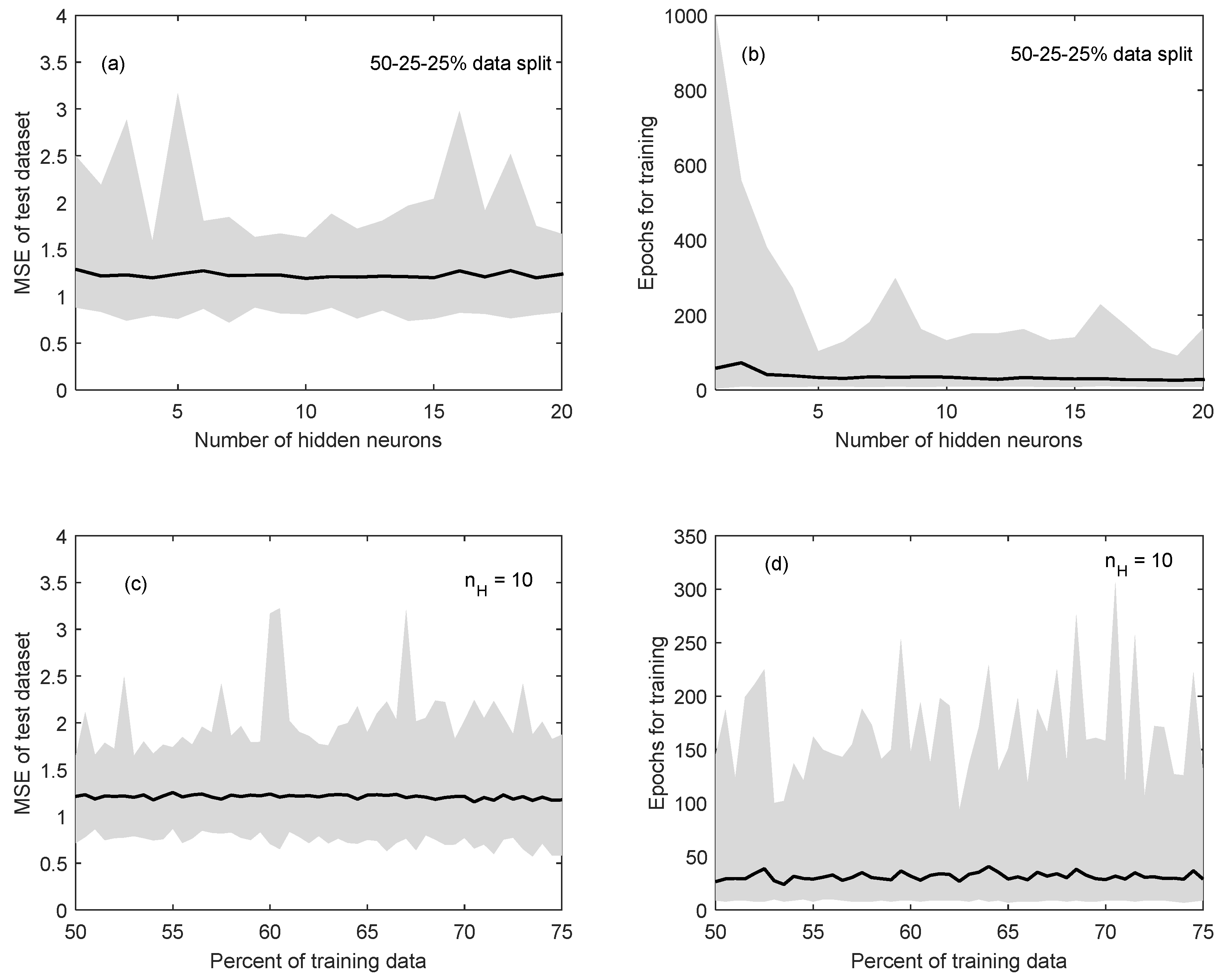
Figure 3.
Sample results of the Fuzzy Neural Network optimisation algorithm to estimate the fuzzy number values of selected weights and biases in the FNN model.
Figure 3.
Sample results of the Fuzzy Neural Network optimisation algorithm to estimate the fuzzy number values of selected weights and biases in the FNN model.
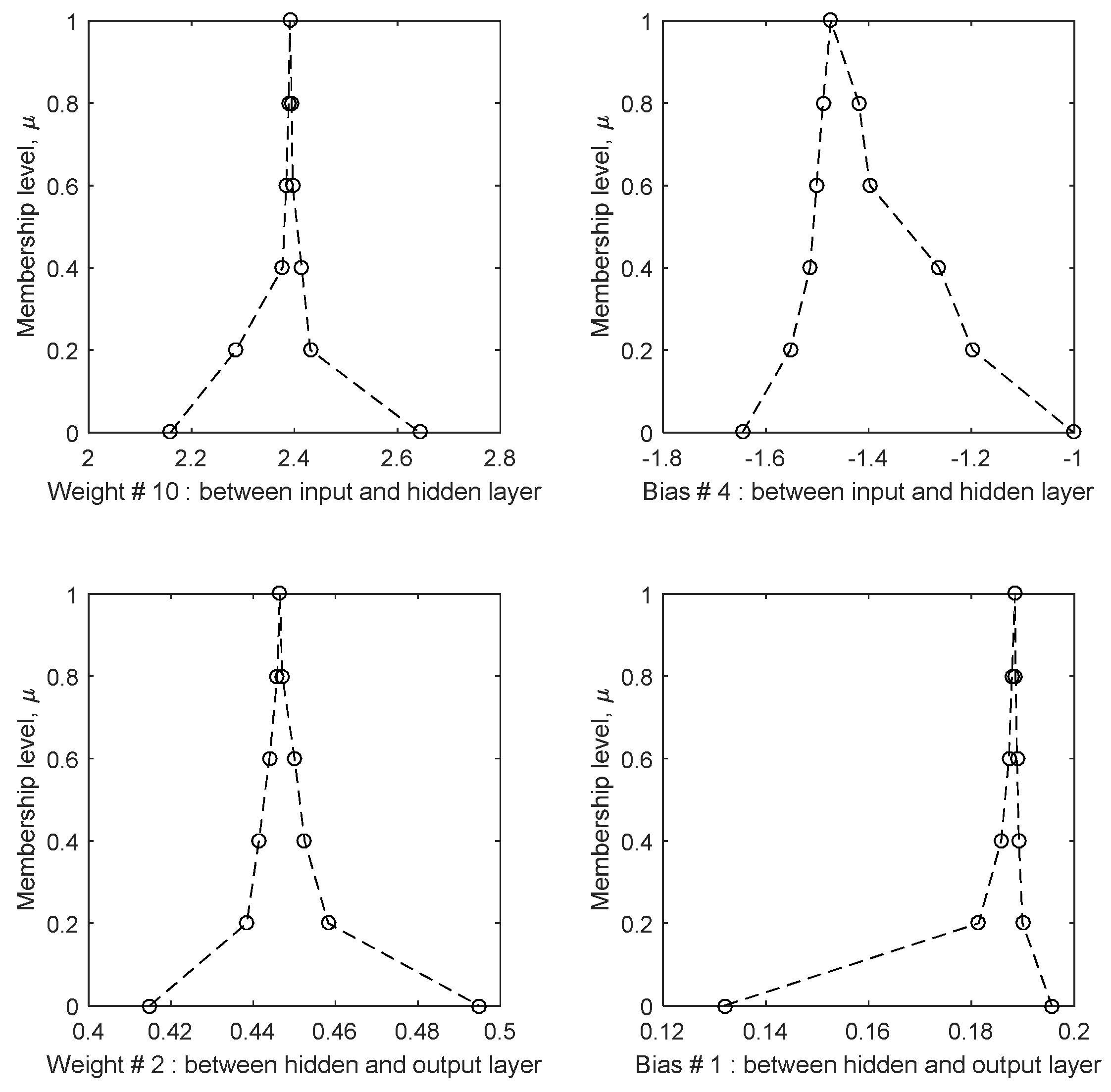
Figure 4.
A comparison of the observed and predicted crisp (black dots) and fuzzy intervals at μ = 0 (grey lines) for minimum Dissolved Oxygen in the Bow River for the training, validation and testing datasets.
Figure 4.
A comparison of the observed and predicted crisp (black dots) and fuzzy intervals at μ = 0 (grey lines) for minimum Dissolved Oxygen in the Bow River for the training, validation and testing datasets.
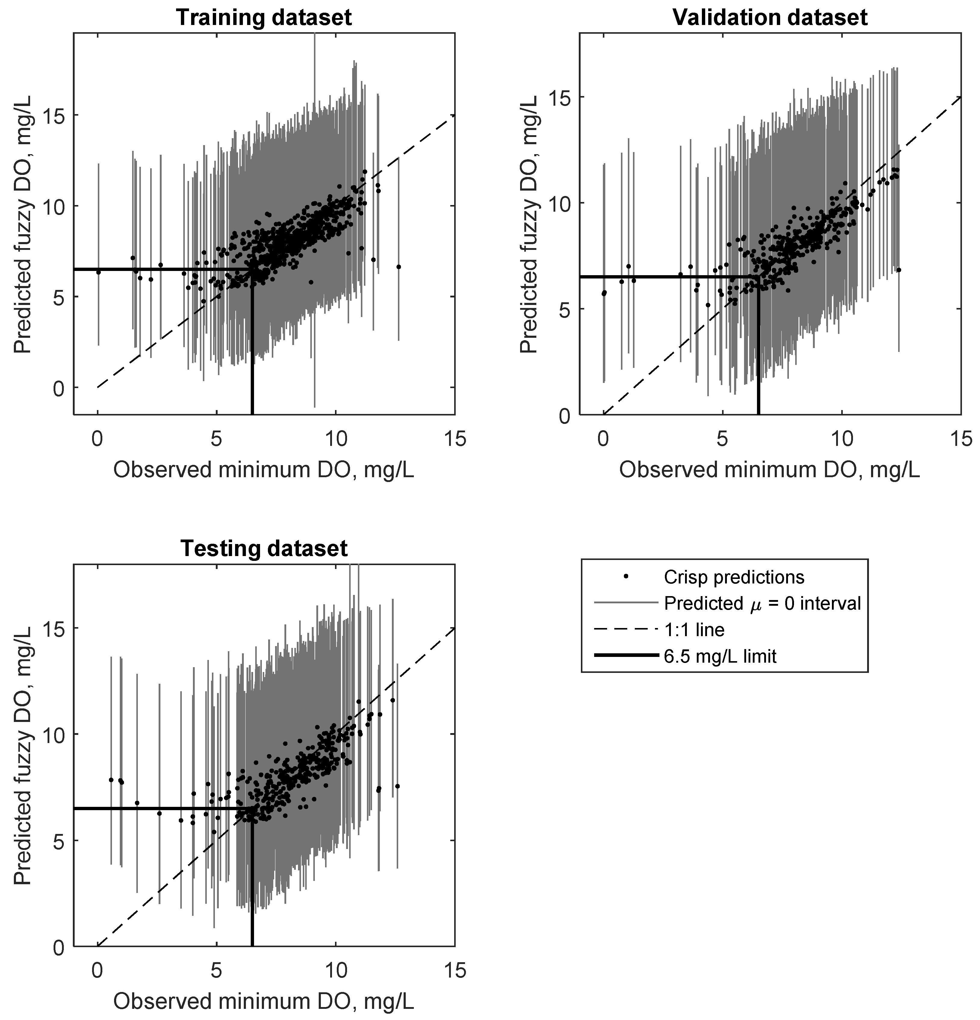
Figure 5.
Time-series comparison of the observations and Fuzzy Neural Network minimum Dissolved Oxygen for 2004 and 2006.
Figure 5.
Time-series comparison of the observations and Fuzzy Neural Network minimum Dissolved Oxygen for 2004 and 2006.

Figure 6.
Time-series comparison of the observations and Fuzzy Neural Network minimum Dissolved Oxygen for 2007 and 2010.
Figure 6.
Time-series comparison of the observations and Fuzzy Neural Network minimum Dissolved Oxygen for 2007 and 2010.
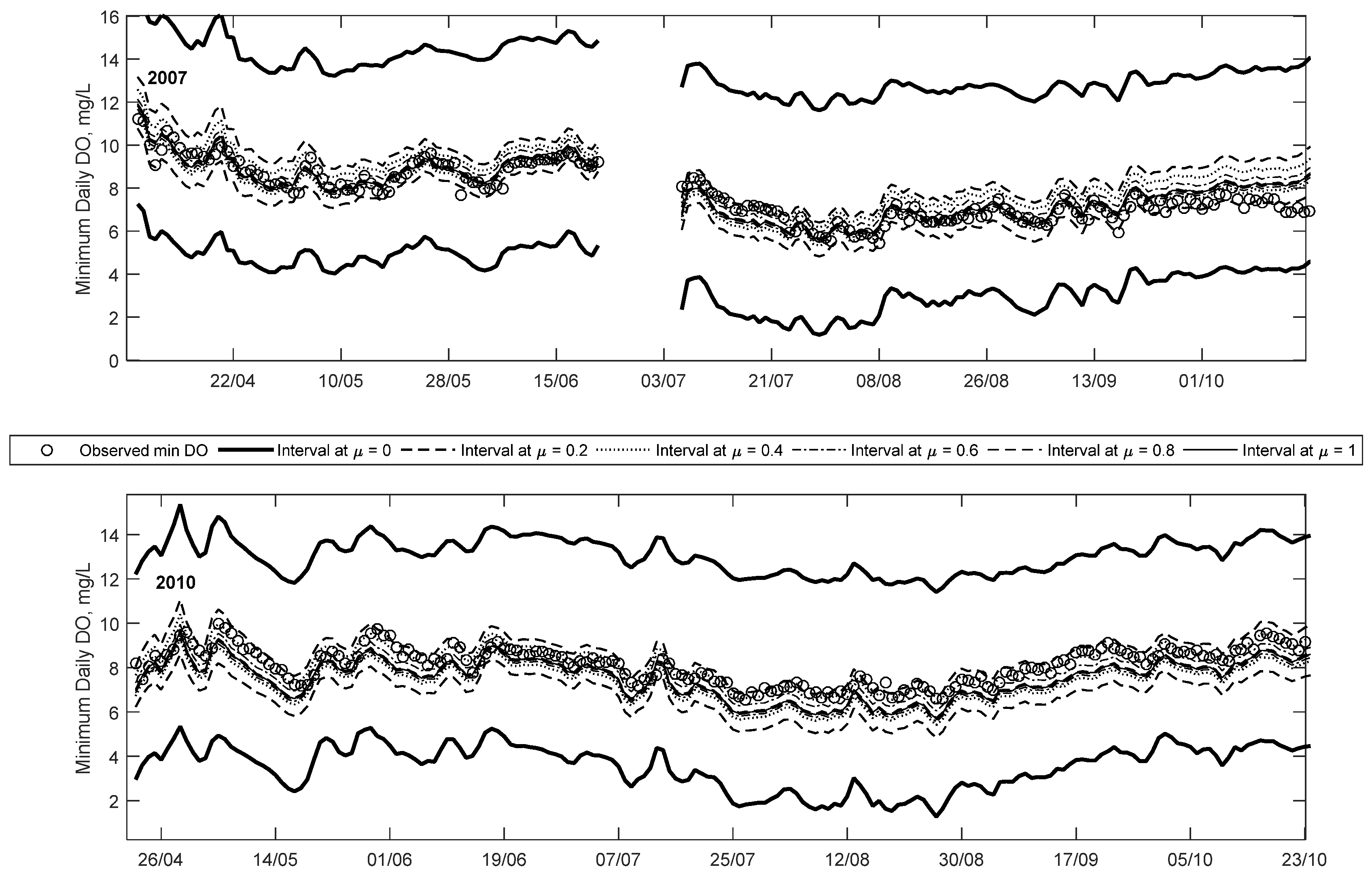
Figure 7.
Detailed view of time series for minimum observed Dissolved Oxygen and predicted fuzzy Dissolved Oxygen for 2004, 2006, 2007 and 2010, corresponding to days with low Dissolved Oxygen events.
Figure 7.
Detailed view of time series for minimum observed Dissolved Oxygen and predicted fuzzy Dissolved Oxygen for 2004, 2006, 2007 and 2010, corresponding to days with low Dissolved Oxygen events.

Figure 8.
Membership functions of the predicted minimum Dissolved Oxygen (dashed line) and observed minimum Dissolved Oxygen corresponding to the lowest Dissolved Oxygen observation for each year (solid black line) between 2004 and 2012.
Figure 8.
Membership functions of the predicted minimum Dissolved Oxygen (dashed line) and observed minimum Dissolved Oxygen corresponding to the lowest Dissolved Oxygen observation for each year (solid black line) between 2004 and 2012.

Figure 9.
Results of the low Dissolved Oxygen identification and risk analyses tool for Dissolved Oxygen less than 5 mg/L.
Figure 9.
Results of the low Dissolved Oxygen identification and risk analyses tool for Dissolved Oxygen less than 5 mg/L.

Figure 10.
Results of the low Dissolved Oxygen identification and risk analyses tool for Dissolved Oxygen less than 6.5 mg/L.
Figure 10.
Results of the low Dissolved Oxygen identification and risk analyses tool for Dissolved Oxygen less than 6.5 mg/L.

Figure 11.
Results of the low Dissolved Oxygen identification and risk analyses tool for Dissolved Oxygen less than 9.5 mg/L.
Figure 11.
Results of the low Dissolved Oxygen identification and risk analyses tool for Dissolved Oxygen less than 9.5 mg/L.


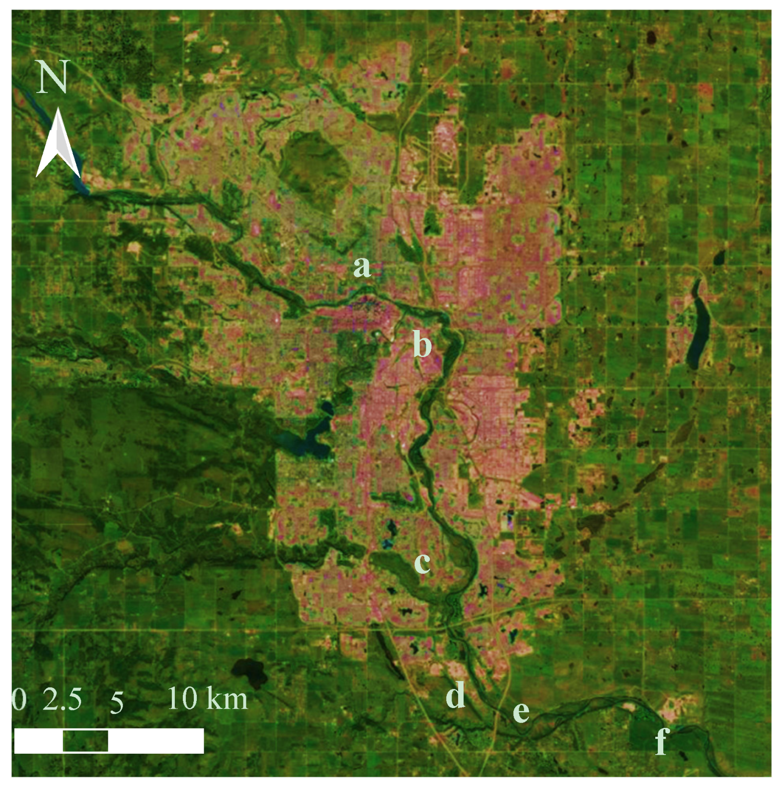
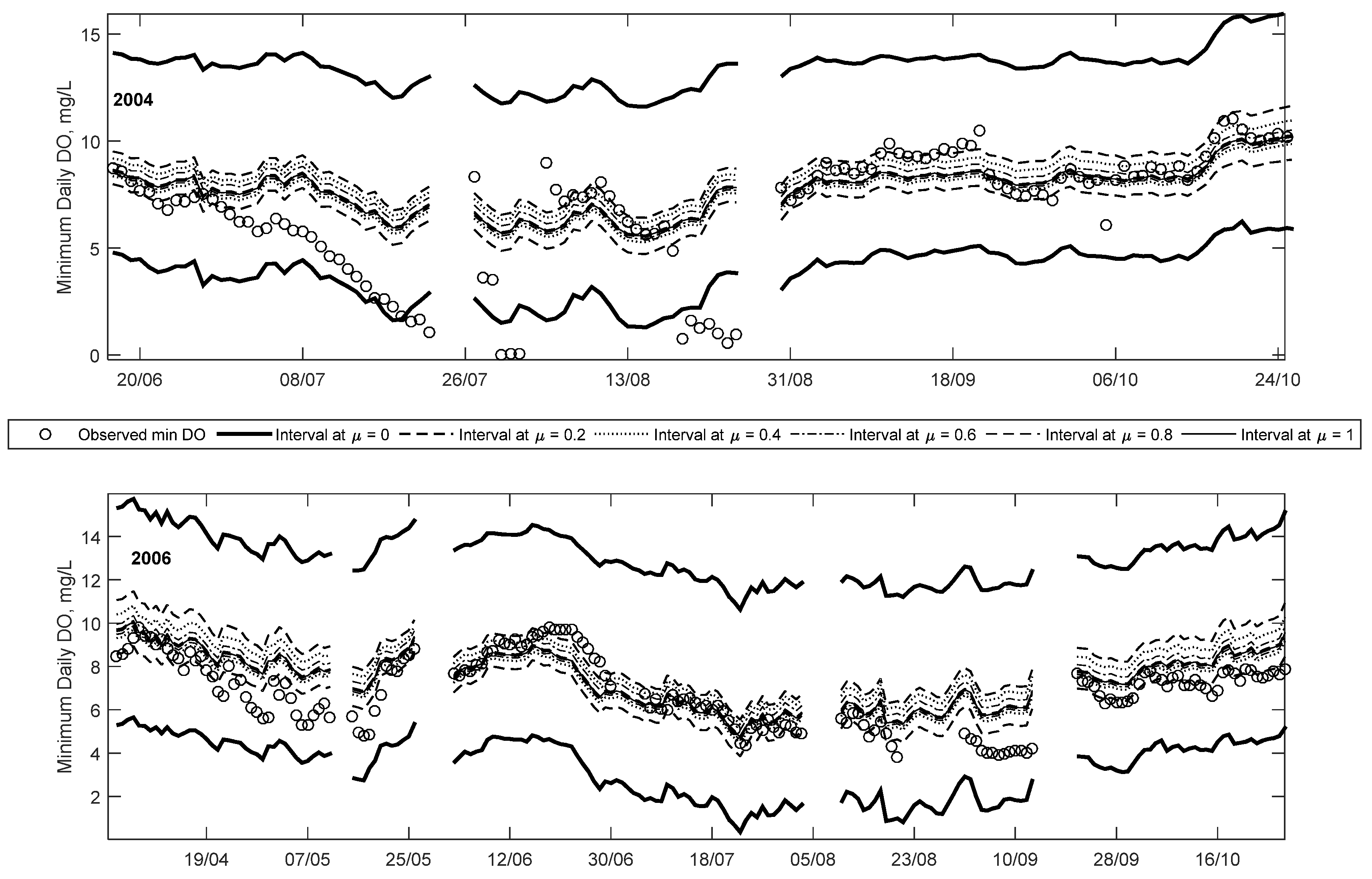
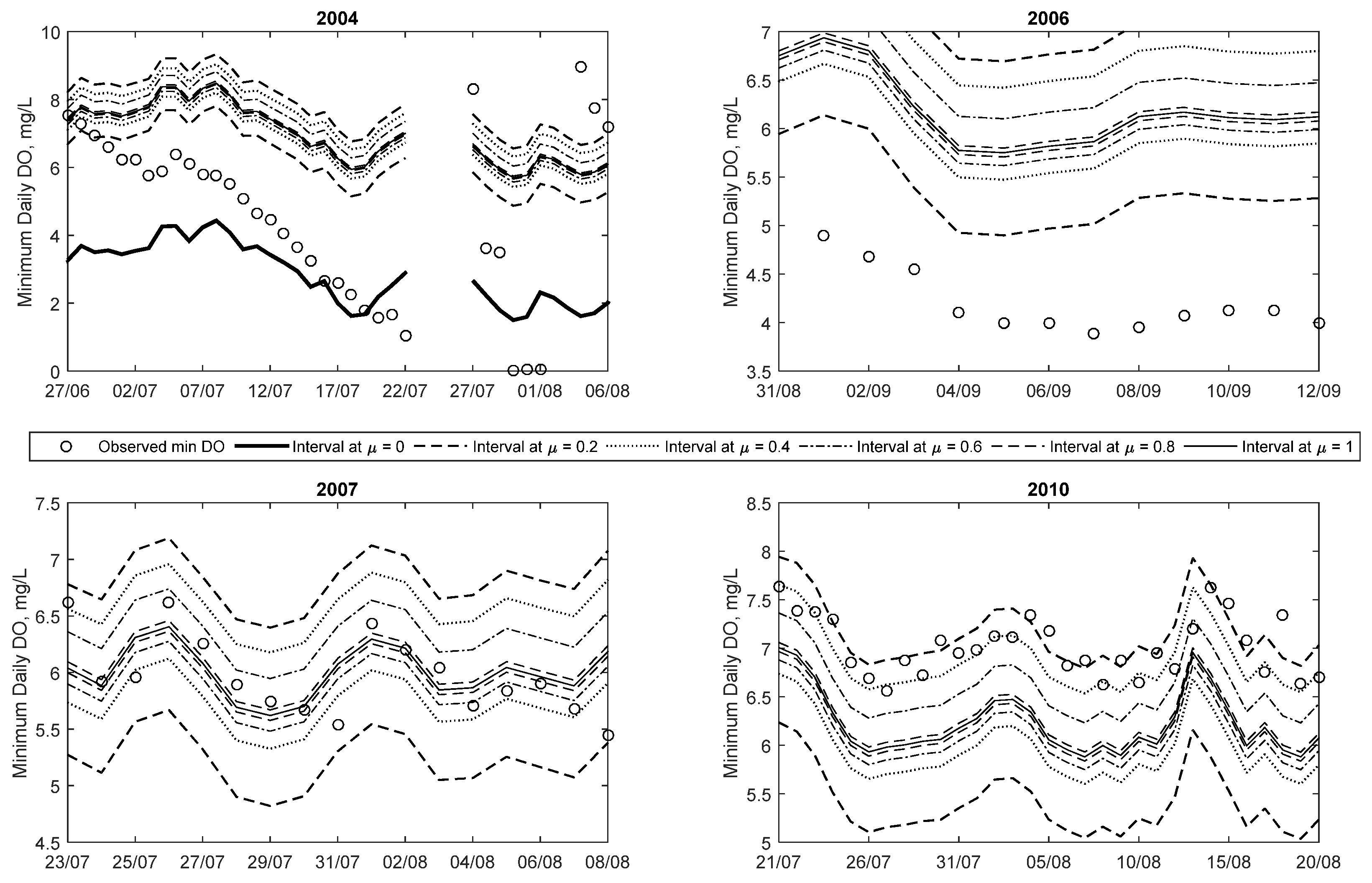
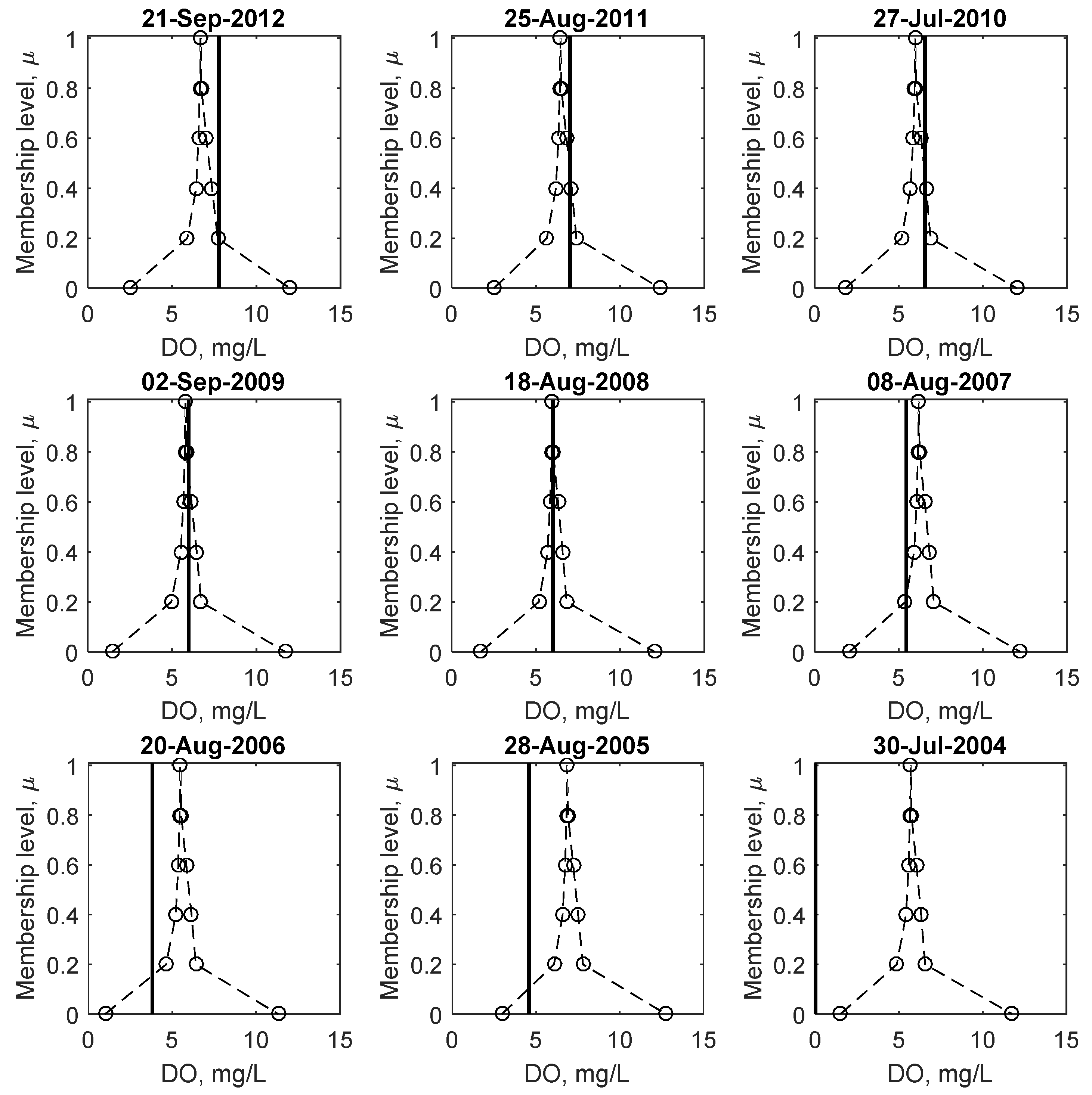
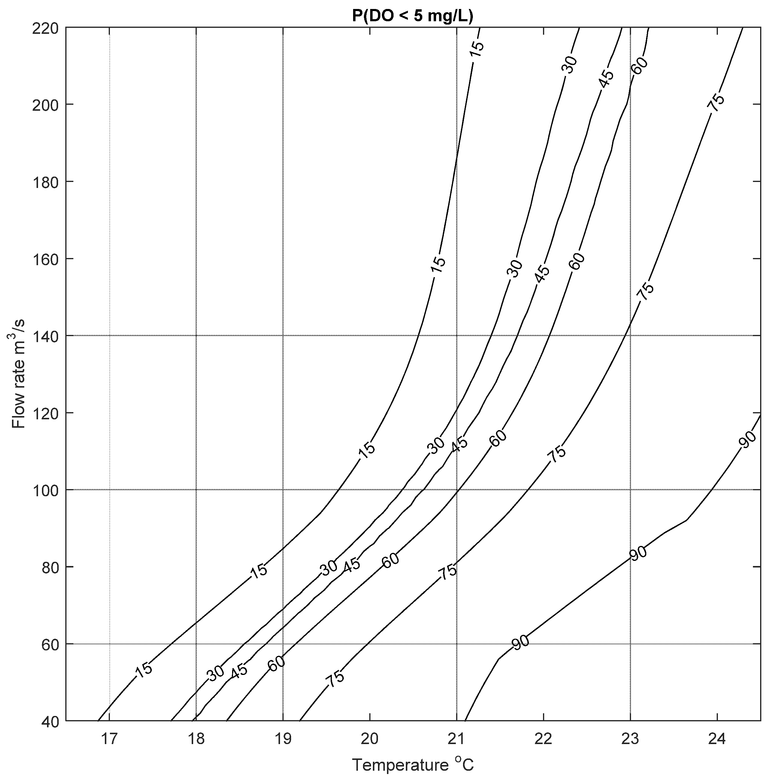
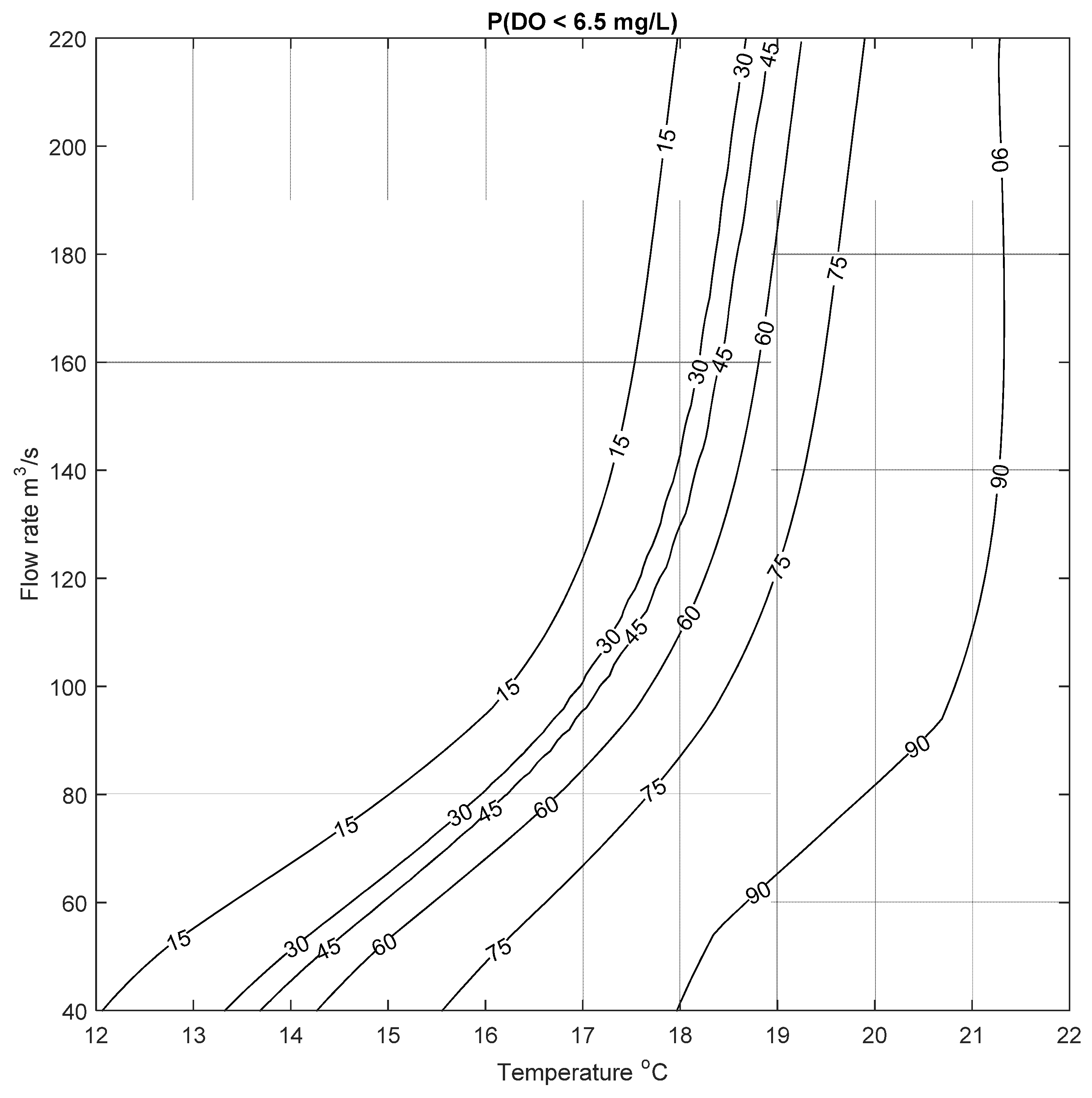
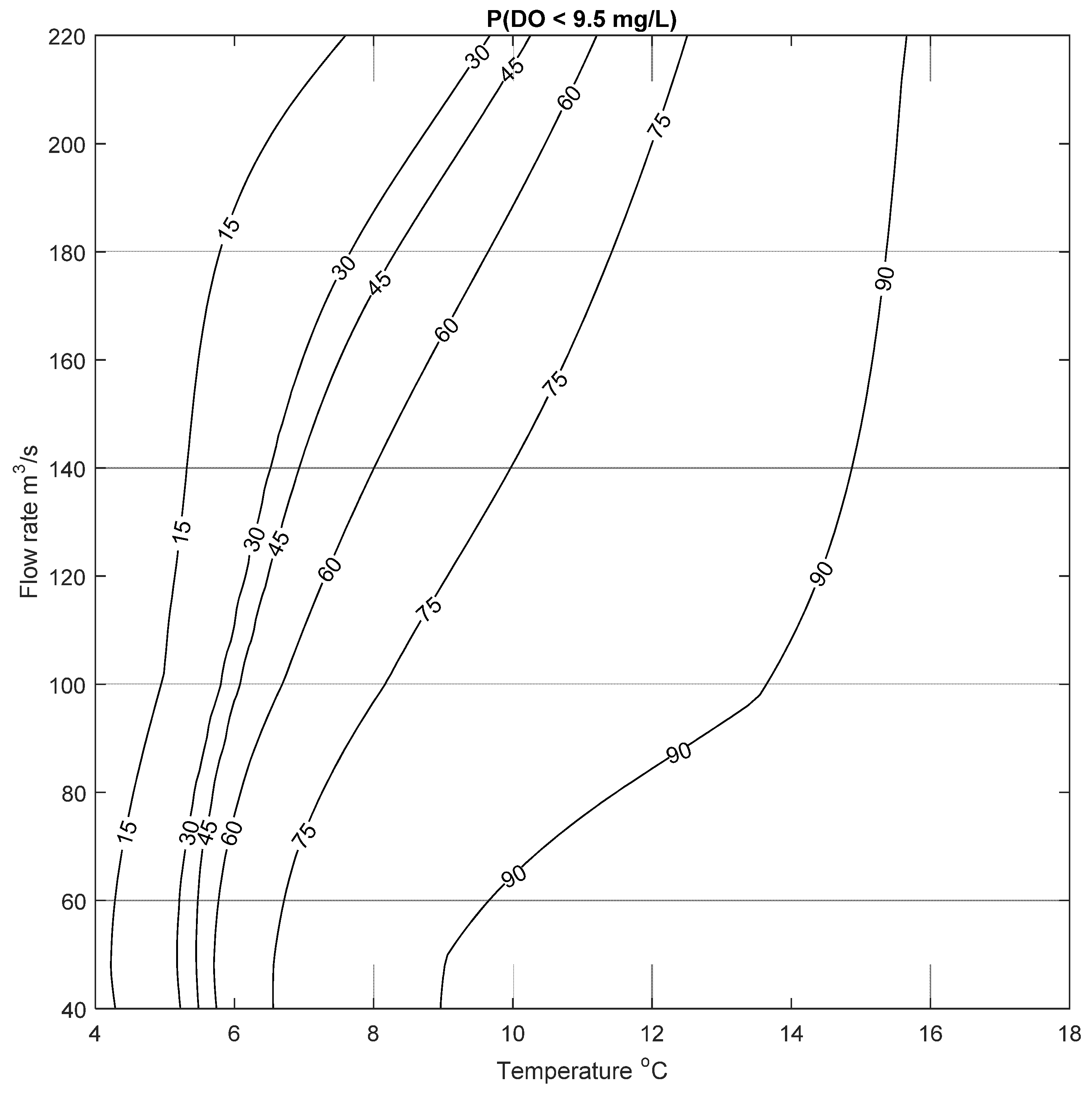
Table 1.
Mean Squared Error and the Nash–Sutcliffe model Efficiency coefficient for the neural network at a membership level equal to 1.
Table 1.
Mean Squared Error and the Nash–Sutcliffe model Efficiency coefficient for the neural network at a membership level equal to 1.
| MSE (mg/L)2 | NSE | |
|---|---|---|
| Train | 1.04 | 0.59 |
| Validation | 1.22 | 0.61 |
| Test | 1.42 | 0.51 |
Table 2.
Percentage of data (%) captured within each fuzzy interval for the Fuzzy Neural Network model.
Table 2.
Percentage of data (%) captured within each fuzzy interval for the Fuzzy Neural Network model.
| μ | Train | Validation | Test |
|---|---|---|---|
| 1.00 | – | – | – |
| 0.80 | 20.02 | 16.10 | 15.85 |
| 0.60 | 40.05 | 34.63 | 33.41 |
| 0.40 | 60.07 | 52.44 | 52.44 |
| 0.20 | 80.10 | 80.00 | 80.24 |
| 0.00 | 99.51 | 98.78 | 99.02 |
© 2017 by the authors. Licensee MDPI, Basel, Switzerland. This article is an open access article distributed under the terms and conditions of the Creative Commons Attribution (CC BY) license (http://creativecommons.org/licenses/by/4.0/).
Share and Cite
MDPI and ACS Style
Khan, U.T.; Valeo, C. Optimising Fuzzy Neural Network Architecture for Dissolved Oxygen Prediction and Risk Analysis. Water 2017, 9, 381. https://doi.org/10.3390/w9060381
AMA Style
Khan UT, Valeo C. Optimising Fuzzy Neural Network Architecture for Dissolved Oxygen Prediction and Risk Analysis. Water. 2017; 9(6):381. https://doi.org/10.3390/w9060381
Chicago/Turabian StyleKhan, Usman T., and Caterina Valeo. 2017. "Optimising Fuzzy Neural Network Architecture for Dissolved Oxygen Prediction and Risk Analysis" Water 9, no. 6: 381. https://doi.org/10.3390/w9060381
Note that from the first issue of 2016, this journal uses article numbers instead of page numbers. See further details here.