
Possibilities of Using Low Quality Digital Elevation Models of Floodplains in Hydraulic Numerical Models


1
Institute of Construction and Geoengineering, Poznań University of Life Sciences, Piątkowska 94, 60-649 Poznań, Poland
2
Institute of Land Improvement, Environment Development and Geodesy, Poznań University of Life Sciences, Piątkowska 94, 60-649 Poznań, Poland
*
Author to whom correspondence should be addressed.
Water 2017, 9(4), 283; https://doi.org/10.3390/w9040283
Submission received: 29 December 2016
/
Revised: 23 March 2017
/
Accepted: 13 April 2017
/
Published: 21 April 2017
(This article belongs to the Special Issue Modeling of Water Systems)
Abstract
:The paper presents a method for the correction of low quality DEMs, based on aerial photographs, for use in 2D flood modeling. The proposed method was developed and tested on the example of the floodplain of the Warta River, which is the third biggest river in Poland. The correction of DEM is based on a series of a small number of measurements using GPS-RTK, which enable calculations of the global statistics like mean error (ME), root mean square error (RMSE) and standard deviation (SD). The impact of DEM accuracy was estimated by using a 2D numerical model. The calculated values of flow velocities, inundation area and volume of floodplain for each tested DEM were compared. The analyses indicate that, after the correction procedure, the predictions of corrected DEM based on poor quality data is in good quantitative and qualitative agreement with the referenced LIDAR DEM. The proposed method may be applied in the areas for which high resolution DEMs based on LIDAR data are not available.
1. Introduction
In recent years, much progress has been observed in flood modeling. This progress has been stimulated by wide availability of 1D and 2D hydraulic models integrated with the geographic information systems (GIS) [1]. Furthermore, wider application of flood models has become possible by the increase in computational resources and large-scale datasets, like elevation and land use data [2,3]. Bates [2] claims that flood inundation research had moved from being a “data poor” to a “data rich” science due to the development of remote-sensing techniques for wide-area topographic mapping. The same author has also concluded that improvement of the terrain data resolution and quality is more important to get a more reliable model than improvement of the representation of physical processes.
A correct representation of the river channel and floodplain geometry, an accurate description of the model parameters, reliable boundary and initial conditions are required to achieve reliable results on the distribution of flow velocities and water levels along the river reach. However, the amount of work and the cost of data preparation required to develop advanced 2D models do not always translate to more accurate results when compared with simplified 1D models. One of the main reason for such inaccuracy is the low quality of the digital elevation model (DEM). Topography is one of the most important factors that has great impact on the hydrologic and hydraulic parameters [4,5,6]. The inaccuracies of DEM are transferred to the final results [7,8,9].
In many countries, for small river basins, no accurate DEMs (based on the relevant measurement techniques, for example, LIDAR (light detection and ranging)) have been developed. Therefore, the commonly-used DEMs are based on aerial photographs and globally available datasets like SRTM (Shuttle Radar Topography Mission) and ASTER (Advanced Spaceborne Thermal Emission and Reflection Radiometer) [10,11,12].
As mentioned earlier, the DEMs used in the flow modeling require determination of their vertical accuracy. The accuracy is most often estimated using global statistics like mean error (ME), root mean square error (RMSE) and standard deviation (SD) [10,13]. These statistics are used when the errors have normal distributions. In other cases, the evaluation of DEM is performed using robust statistical methods, in which the median value, normalized median absolute deviation, the 68.3% quantile and 95% quantile are calculated [14]. However, both methods are global indicators and do not account for the spatial variability of the errors [15]. To describe the spatial distribution of the errors, efforts are made to connect errors with the parameters describing the investigated area, such as slope, aspect and curvature [16]. Another approach is to use the global and local spatial autocorrelation indices, namely Moran’s I and the Getis–Ord G indices.
Walczak et al. (2016) [10] and Gichamo et al. [13] have proposed methods to correct freely-available, satellite-based DEMs. In the propositions of both authors, the vertical error correction is based on the determination of the average error calculated using field measurements. Walczak et al. [10] compared four DEMs based on various data sources (SRTM, ASTER GDEM, LIDAR and aerial photographs) to calculate polder retention capacity. The authors concluded that the accuracy of ASTER or SRTM DEMs is generally insufficient for flood modeling, especially for modelling polders’ capacity as flood-protection systems. The same authors emphasized that in the absence of a high resolution DEM based on LIDAR data, the DEM developed on the basis of aerial photographs can be used after some correction based on field measurements. Saksena and Merwade [17] have analyzed the impact of DEM resolution and accuracy on the flood inundation mapping. They pointed out that water surface elevations (WSE) along the stream and the flood inundation area are in a linear relationship with both DEM resolution and accuracy. The application of this approach has shown that improved results can be obtained from flood modeling by using coarser and less accurate DEMs, including those based on public domain datasets.
The development of a DEM for flood modelling is a great challenge due to the problems related to interpolation of river bathymetry and its subsequent integration with the floodplain [11]. Gichamo et al. [13] have presented two approaches for the extraction of river cross-sections from a satellite-based ASTER DEM to be used in 1D river modeling. In the first method, the dimensions of triangular cross-sections were determined from the DEM, and subsequently, they were corrected for vertical bias based on elevation error. In the second approach, an optimization routine applied to conceptual flow routing equations was proposed to identify the equivalent channel geometry parameters from the observed flow and water levels for a given flood event. Elevation value differences between the ASTER GDEM and a high resolution and high vertical accuracy DEM available for a limited portion of the river reach were calculated at a number of points along the river channel and floodplain. The authors concluded that the vertical error correction by adjusting the cross-sections for the average error at these points produced a considerable improvement in the model outputs.
Yan et al. [3] have shown tremendous progress in using remote sensing data in advanced flood inundation modelling. In particular, low cost space-borne data could be used to support hydraulic model building, as well as for model calibration and evaluation. The satellite products yield valuable information such as land surface elevation, flood extent and water level, which could be potentially used for flood modeling studies. The major scientific challenges in the last two decades have been to explore remotely-sensed data towards building, calibration and evaluation hydraulic models. Topographic data are some of the most important input data for hydraulic modeling. These data are also considered as some of the most significant sources of uncertainty in hydraulic modeling. Presently, a great challenge still is the integration of low cost space-borne data and airborne sensing data with the ground-based observations and estimation of uncertainties related to hydraulic modelling.
The finite element method (FEM) or the finite volume method (FVM) is usually used to solve the differential equations describing the flow in a 2D or 3D space. These methods require a mesh of an appropriate quality and the use of special techniques. These techniques must ensure the reduction in errors arising at the DEM generation stage [11] and must minimize the number of characteristic points describing the area without significant simplification [18].
The aims of this paper were: (1) the development a method for the correction of low quality DEMs based on aerial photographs for use in 2D flood modeling; (2) the development of a method for the optimization of mesh generation; and (3) the assessment of the impact of DEM accuracy on the flood modeling results.
2. Materials and Methods
In this paper, the following definitions were used. Original DEM is the model developed on the basis of aerial photographs in the scale of 1:26,000. Corrected DEM is the model developed on the basis of original DEM by correction of vertical errors with supplementing the bathymetric data. Optimized DEM is the model developed on the basis of corrected DEM by optimizing the mesh division into the elements. Reference DEM is the model developed on the basis of LIDAR data.
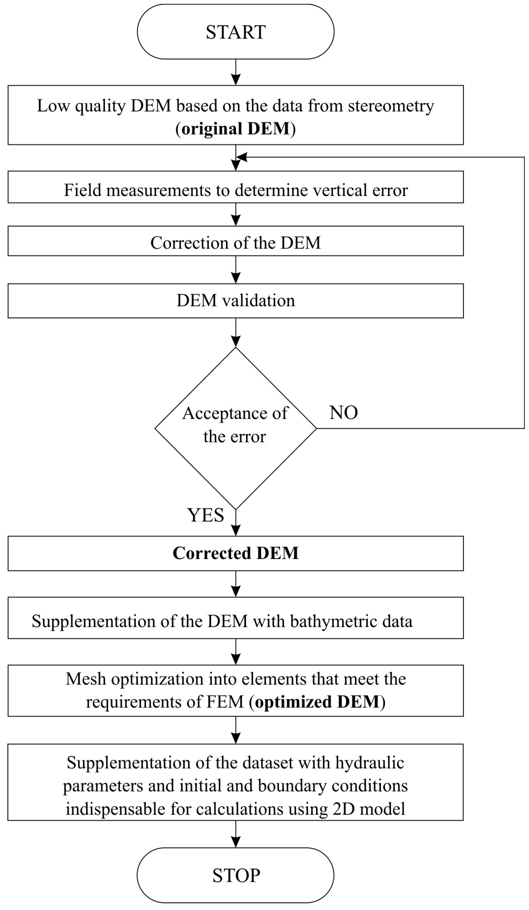
The stages of the process are shown in Figure 1. The use of the approach proposed ensures not only the quality of data included in the original DEM, but also the mesh division into elements, which influences the error generated by the method used for solving the equations that describe the open channel flow. The method involves the use of a small number of field measurements for correction of the vertical error of DEM.
2.1. Study Site Description
The proposed method was developed and tested on the basis of the floodplain of the Warta River, which is the third biggest river in Poland. The selected river reach is 2.22 km long, and it is located between 351.82 and 354.042 km of the Warta River (Figure 2). The average width of the river valley is 490 m, and the main channel width varies from 50 to 84 m. The floodplains are covered with grass and shrubs and trees.
2.2. DEM Availability and Description
The original DEM used in this paper is based on aerial photographs from 2009 in the scale of 1:26,000. The reference DEM is based on LIDAR data obtained from the National Defense Computer System (in Polish, Informatyczny System Ochrony Kraju (ISOK)). The density of the LIDAR cloud is 6 points per square meter. The mean error of the original DEM varied from 0.4 to 0.9 around Poland [19]. The mean error of reference DEM varied from 0.1 to 0.2 m.
2.3. Field Measurements
The measurements were performed using the SOKKIA GRX-1 GNSS receiver and RTK (Real Time Kinematic) system. This system permits reception of the GPS and GLONASS signals with RTK correction through the GSM network. The measurement accuracy of the applied device was 10 mm + 1 ppm for the X and Y coordinates and 20 mm + 1 ppm for the Z coordinate. During field measurements, we used GUGiK geoid2001 (GUGiK is the Head Office of Geodesy and Cartography) [20] providing results with the accuracy of ±1.8 cm [21]. The assessment of DEM quality was performed on the basis of the 450 measurements. The first set of 400 measurements was used to assess the quality of the original DEM and its correction. The corrected DEM was validated on the basis of 50 additional measurements performed in a single cross-section (Figure 2).
2.4. Assessment of the DEM Accuracy
In the first stage of the analysis, the errors were calculated as the differences between the elevations given in the original DEM and those measured in the field. In the next stage, the distribution of the original DEM errors was checked against the normal one; this step was performed graphically and by means of the Shapiro–Wilk test. The original DEM quality was evaluated on the basis of the commonly-used global statistical measures: mean error (ME), root mean square error (RMSE) and standard deviation (SD).
To examine the extent of error clustering, the Moran and Getis–Ord measures were used. The possible values of Moran’s statistic range from −1 to 1. Positive values indicate spatial clustering of similar values, while negative values indicate clustering of dissimilar values. The Getis–Ord statistics was used to measure the concentrations of high or low error values for the entire study area. A high index value indicates that high error values are clustered within the study area. A low index value indicates that low error values tend to cluster [22].
In the final stage, the relationships between the error and (1) the type of land use within the floodplain area and (2) the topographic indices, i.e., slopes, aspect and curvature, were established.
The errors were analyzed in relation to the structure of land use in the floodplain zone (low and medium size vegetation) and in relation to the landscape features (old river beds, embankments, flood valley banks). The structure of land use was determined on the basis of orthophotomaps. No correlations were detected between the errors and the structure of land use and landscape features.
To describe the errors’ magnitudes with the parameters characterizing the investigated area, such as slope, aspect and curvature, the method proposed in [16] was used. The primary terrain attributes, e.g., slope, aspect and curvature, were calculated directly from the DEM. The values of slope, aspect and curvature were extracted to the points at which the errors were calculated. Then, correlations were searched between the errors and each of the primary terrain attributes. No correlations were detected between the errors and slope, aspect and curvature.
Statistical calculations were performed by means of the Statistica 10 software package (StatSoft), and the characteristics of the spatial error distribution were obtained using ArcGIS 9.3.1. (ESRI), as well as GeoDa 0.9.5-i5 [23].
2.5. Bathymetry Supplementation
As mentioned above, DEMs do not provide information about river bathymetry. To get these data, the cross-sections of the river channel must be determined. The measurements were made for the total of 13 cross-sections of the Warta. Their locations are shown in Figure 2. The bathymetric measurements were recorded using the ADCP StreamPro velocity profiler. Therefore, the assessment of the DEMs’ accuracy described in Section 2.4 must be made prior to the integration of bathymetric data with the floodplain data. The algorithm used to generate the river bathymetry was based on the linear interpolation of the points between the surveyed cross-sections (Figure 3b). The DEM (Figure 3a) supplemented with bathymetry is shown in Figure 3c.
2.6. Mesh Generation and Optimization
The mesh generated on the basis of the original DEM is highly irregular, both in terms of its density and the shape of its elements (Figure 3a) and cannot be directly used for flood modeling. Moreover, an appropriate density in crucial sub-areas is also of importance. Further, the appropriate method of mesh generation based on the available data must be chosen [24,25,26,27,28]. In some situations, even when the measurement data resolution is satisfactory (e.g., LIDAR), problems may occur in the modeling of certain elements of the flow area, such as embankments, hydraulic structures outlines, bridge heads and pillars. These elements often cause an abrupt increase in one of the dimensions [29].
The main channel bathymetry consists of regular elements due to the interpolation procedure used to obtain the intermediate cross-sections. However, the floodplain includes many highly irregular elements (Figure 3c), which affect the accuracy of the solution based on the finite elements methods (FEM). For proper application of the method used to solve 2D unsteady flow problems, the mesh dividing the area into elements should be as regular as possible, and its density should increase in the places where the geometry of flow undergoes abrupt changes (e.g., at the borderline between the watercourse bed and the floodplain, steep banks, embankments, etc.). High nonlinearity can often lead to large local errors and deteriorate the convergence of the iteration solution-finding process [30]. The mesh must then be optimized in terms of: (1) projection of the area and the elements of the technical infrastructure; and (2) the shape of its elements, high density zones and mesh resolution. Numerous algorithms have been proposed for this purpose [18,31,32]. The influence of mesh density on the DEM is considerable as depending on the type of generalization, the incorrect choice of mesh density may lead to the loss of certain detail features in the topographic profile [6,33,34]. Smaller elements allow a better mapping of the velocity field or better representation of the boundaries [35], which is particularly important in urbanized areas [36,37].
This convergence problem may be solved by creating a mesh that would meet the criteria required by the FEM and then assigning the elevation values interpolated from the DEM to the nodes (Figure 3d). In the process of FEM mesh generation, it is important to provide correct representation of the linear elements, such as the water-course bed, embankments, risings and bridge heads. Thus, the process should ensure the possibility to determine the sub-areas that would be well fitted to the surface topography while ensuring coherence and smooth connectivity between these sub-areas in the entire area of flow. Such a mechanism has been implemented, among others, in the GEMOF (in Polish Generator Elementowego MOdelu Filtracji) program [31], applied to generate a mesh fulfilling the requirements of the FEM used to numerically solve the shallow water equations.
2.7. Impact of DEM Accuracy on 2D Hydraulic Modeling
In the final part of this study, the impact of the DEM accuracy on hydraulic modeling results was evaluated. Flood modeling was performed using the RISMO2D (RIver Simulation MOdel) system [38]. This system allows simulation of 2D flow described by the well-known shallow water equations, which can be written as follows:
Momentum equation:
Continuity equation:
where Vx, Vy are integrated over depth flow velocity (m·s−1), α1, α2, α3 are correction coefficients accounting for the fact that the average of the product of two functions is not the product of the averages (-), h water level (m), ρ water density (kg·m−3) and τx0, τy0 bottom-shear stresses (kg·m−1·s−2).
To solve Equations (1) and (2), the finite element method or the finite volume method (FVM) can be used in the RISMO2D system. The calculations provide the elevation of the water table and the components of the velocity vector. The calculations were performed for three different variants. The variants applied in this study were based on the original DEM, corrected DEM and reference DEM. In all variants, the DEMs were supplemented with the main channel bathymetry. It is important to note that all three variants have the same resolution of the mesh (78,960 nodes and 156,837 elements) and the shape of elements that meet the FEM requirements. Elevations of the mesh points were assigned using the inverse distance weight. In this way, the error resulting from the using the computational method (FEM) was the same in all simulations.
A hydraulic model requires defining boundary conditions and the values of roughness coefficients for the floodplain and the main channel. These data for the 2D model were obtained from the 1D unsteady flow routing model for a 50 km-long reach of the Warta section from the gauge stations Sławsk to that in Nowa Wieś Podgórna located at kilometers 392.2 and 342.6, respectively. The unsteady flow modeling system SPRUNER (in polish System Prognozowania Ruchu Nieustalonego w Rzekach) [39], based on the Saint Venant set of equations (1D-SVE), developed at the Faculty of Environmental Engineering and Spatial Management at the University of Life Sciences in Poznan, has been applied to carry out 1D modelling. In the SPRUNER system, 1D-SVE are approximated using the Preissmann implicit finite differences scheme [40] and are solved numerically using the Newton–Raphson iteration technique. The 1D model was calibrated on the basis of the data for the spring spate of 2011 and verified on the basis of the data for the spring spate of 2013. The calibration procedure was carried out using the predictor-corrector technique. The study area was represented in the 1D model by 5 cross-sections, whose locations are shown in Figure 2.
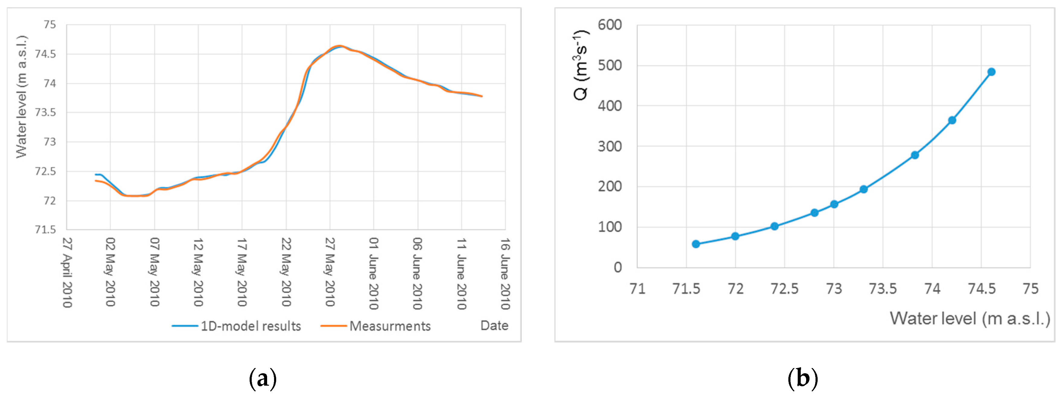
1D model calculations were carried out for the flood of year 2010. Verification of the 1D model was made with the data from the gauge station located at 352.17 km of the Warta River. The calculated and measured water levels hydrographs are shown in Figure 4a.
The average difference between the measured and calculated values was 0.045 m, and the correlation coefficient was equal to 0.997. The results obtained from the 1D model allowed us to establish a relationship between the flow rate and the water level in the cross-section 351.82 (Figure 4b), which was used to determine the boundary conditions for the 2D model.
The values of the roughness coefficient for the 5 cross-sections located within the study site area were also used. They were assigned to the elements of the FEM mesh with the help of the linear interpolation procedure. The RISMO2D system enables calculations for both steady and unsteady flow conditions. As the calculations were time consuming, nine different 2D flow simulation for each variant under steady state conditions were performed. For each variant, the roughness coefficients had the same value in all simulations. The simulations allowed estimation of the volume (VEE) and area (AEE) mapping error, as well as a comparison of velocity field distribution for the three previously mentioned variants.
VEE and AEE were calculated according to the formulas:
where A and V are the values computed for the original and corrected DEMs.
3. Results and Discussion
3.1. DEM Accuracy Assessment
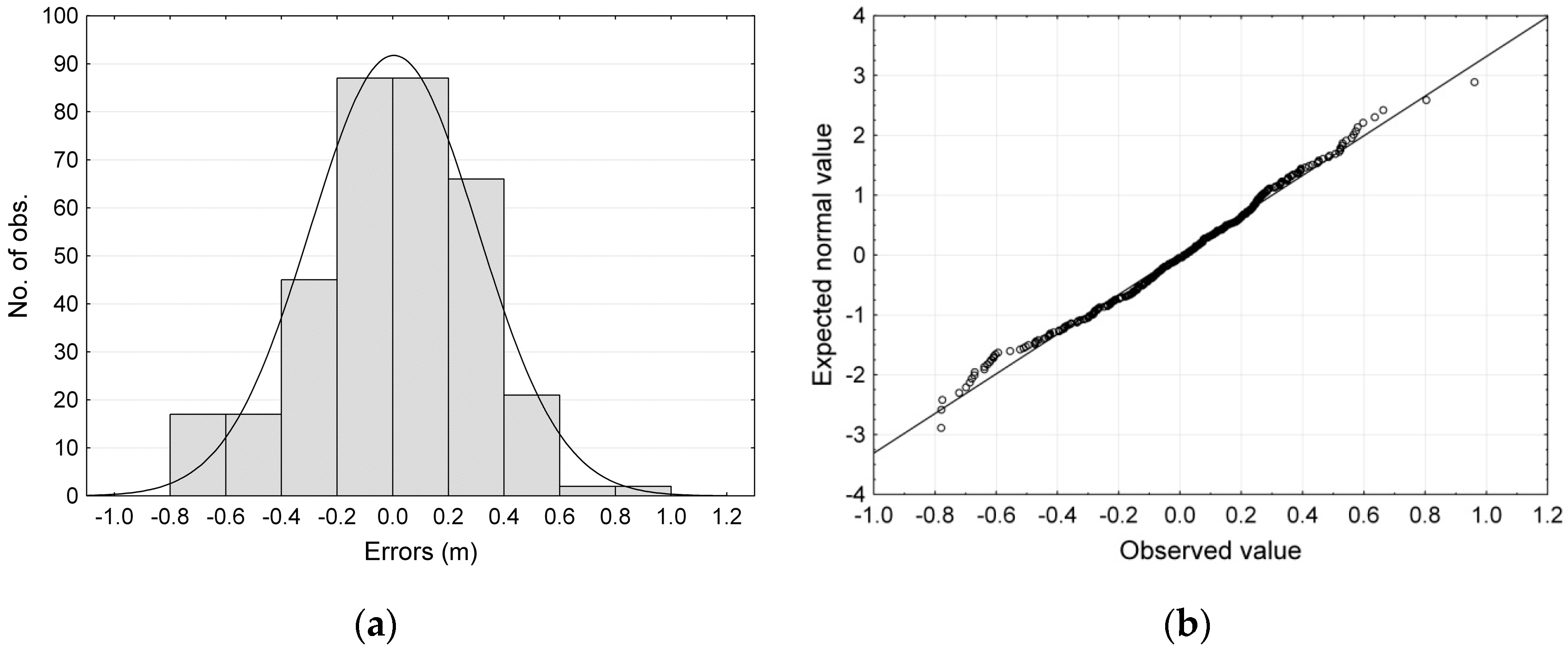
The first stage of the analysis consisted of calculating the differences in elevation between the points measured in the field by means of SOKKIA GPS-RTK and those obtained from the original DEM. The differences varied from −0.21 m to 1.53 m, and their distribution was approximately normal. The RMSE of the original DEM model was 0.63 m, with the random error SD equal to 0.30 m and the systematic error ME equal to 0.56 m. Due to the systematic error, all of the elevations values of the original DEM were lower than the measured values. The errors of the DEM and their distribution after performing a correction to the systematic component are shown in Figure 5a,b, respectively.
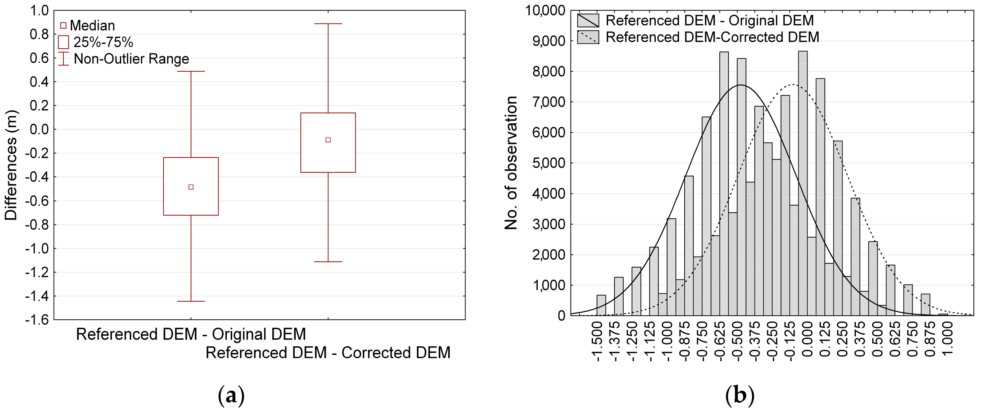
In the next stage, the original DEM and corrected DEM were compared with the reference DEM obtained from LIDAR data. Statistical analysis was performed using the elevation differences read at 61,839 points. First, the extreme and outlier values were rejected, which jointly constituted approximately 5% of all of the points. The differences between the original DEM and the reference DEM varied from −1.49 m to 0.56 m, with the mean value of −0.48 m and the standard deviation of 0.39 m (Figure 6a). The corrected DEM was processed in the same manner. In the corrected DEM, the mean error was 0.03 m, and the differences between the elevations ranged from −1.12 to 0.89 m. The differences between the models had a distribution resembling the normal one (Figure 6b).
The relationship between the elevation points from the original and corrected DEM and the reference DEM are shown in Figure 7a,b respectively. In the second stage of DEM correction, the spatial error distribution and the relationships between the error and the type of land use and the relief were analyzed. The analysis based on the Moran, Getis and Ord correlation coefficients indicate no autocorrelation of the errors. Besides, no correlations were detected between the errors and the structure of land use and landscape features. In view of the above, a correction of the systematic error was made. DEMs’ accuracy is crucial in modeling floods in small and medium rivers, for which no LIDAR-based models exist.
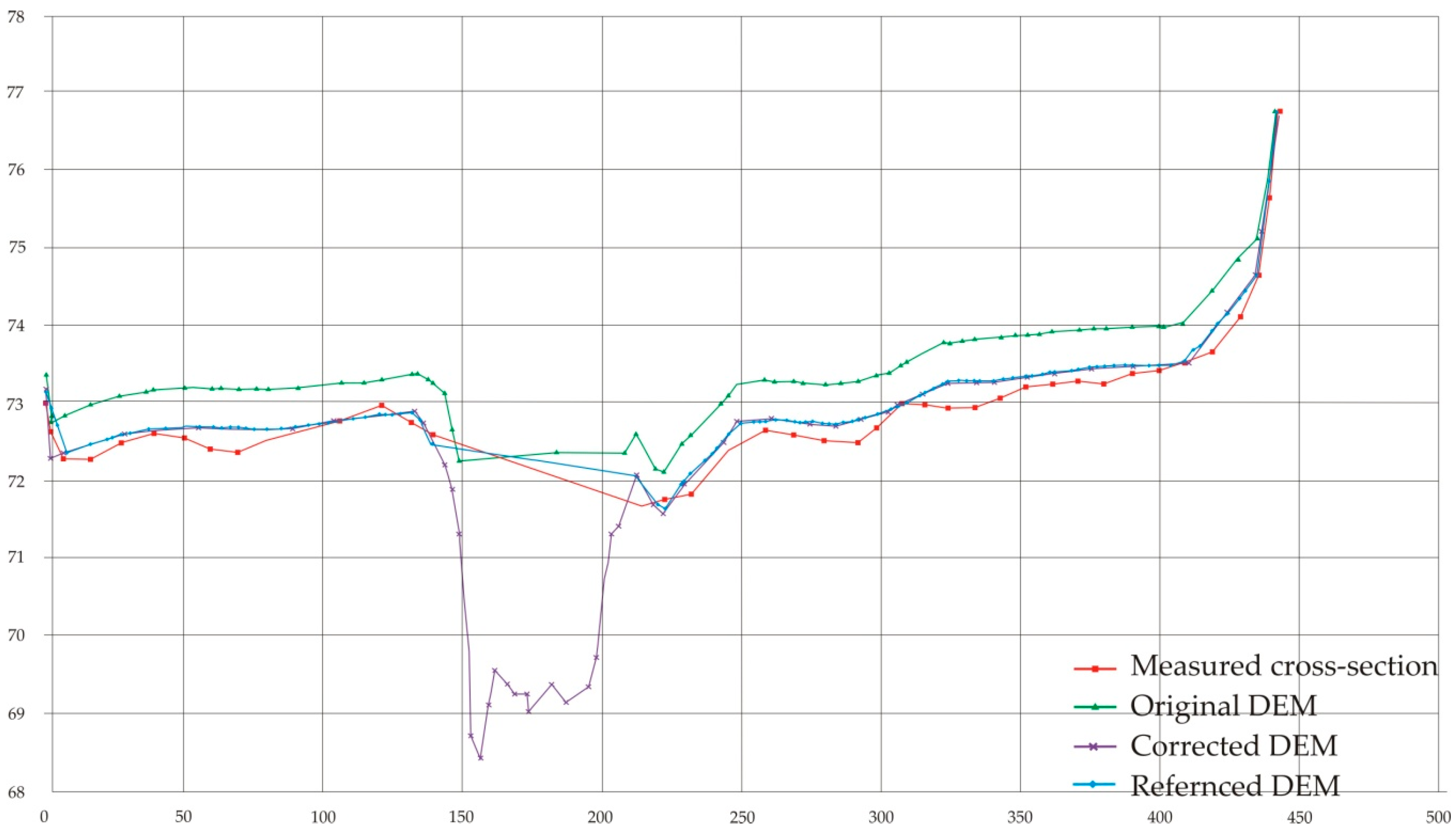
In the final stage, the corrected DEM was validated on the basis of the independent measurements not used previously for its correction. Figure 8 shows a comparison between DEMs at a selected cross-section. The analyses revealed a good agreement between the DEM developed according to the proposed method (Figure 2) and the reference DEM. Moreover, the generation of the FEM mesh and the assignment of the DEM-based elevation values to the mesh had no significant impact on the elevation model of the investigated area (Table 1).
3.2. Results of the 2D Model Simulation
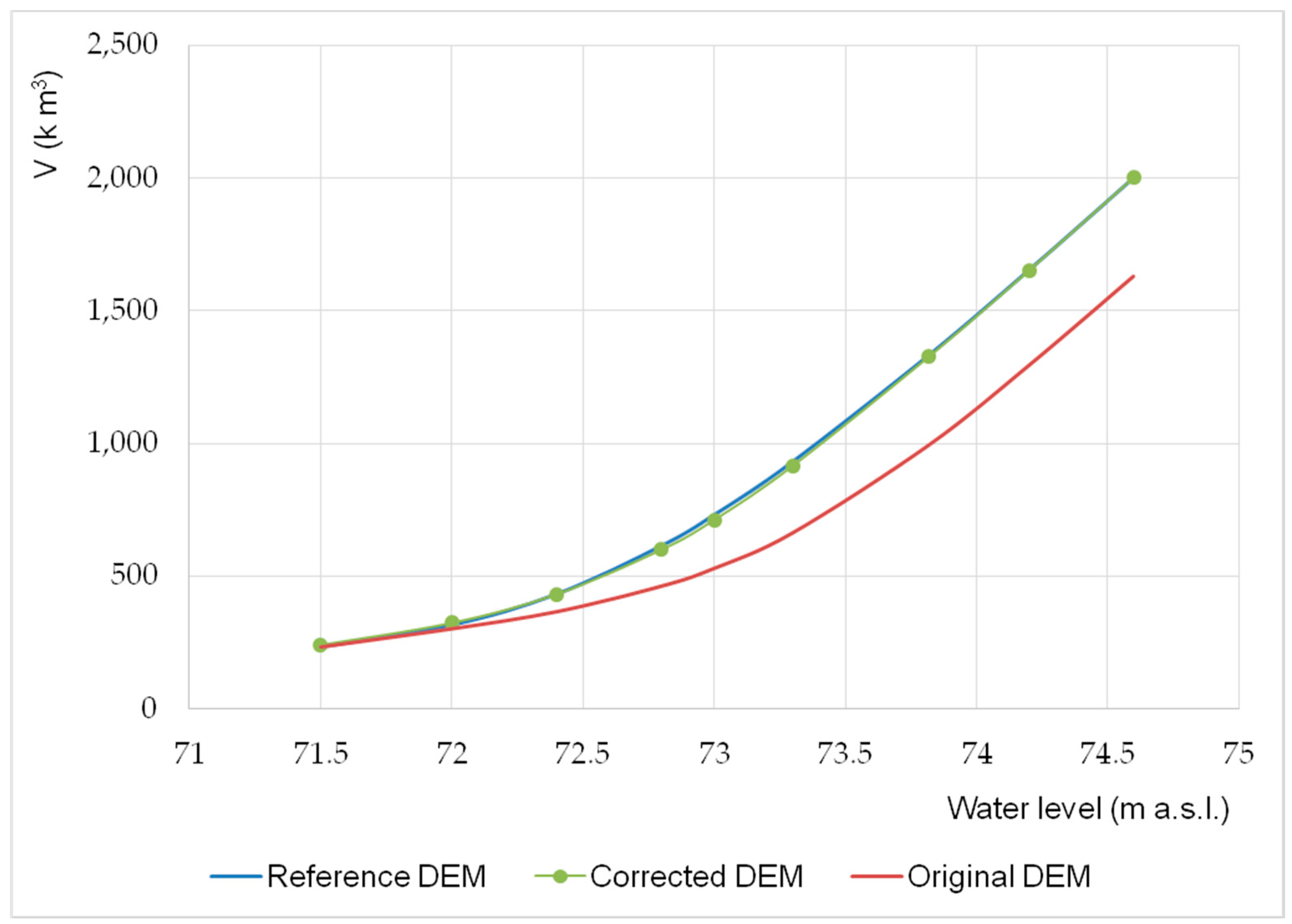
The summary of results obtained from all simulations are presented in Table 2. The relationship between the water level at the cross-section 351.820 and the volume of accumulated water in the area of interest determined on the basis of the calculations is shown in Figure 9.
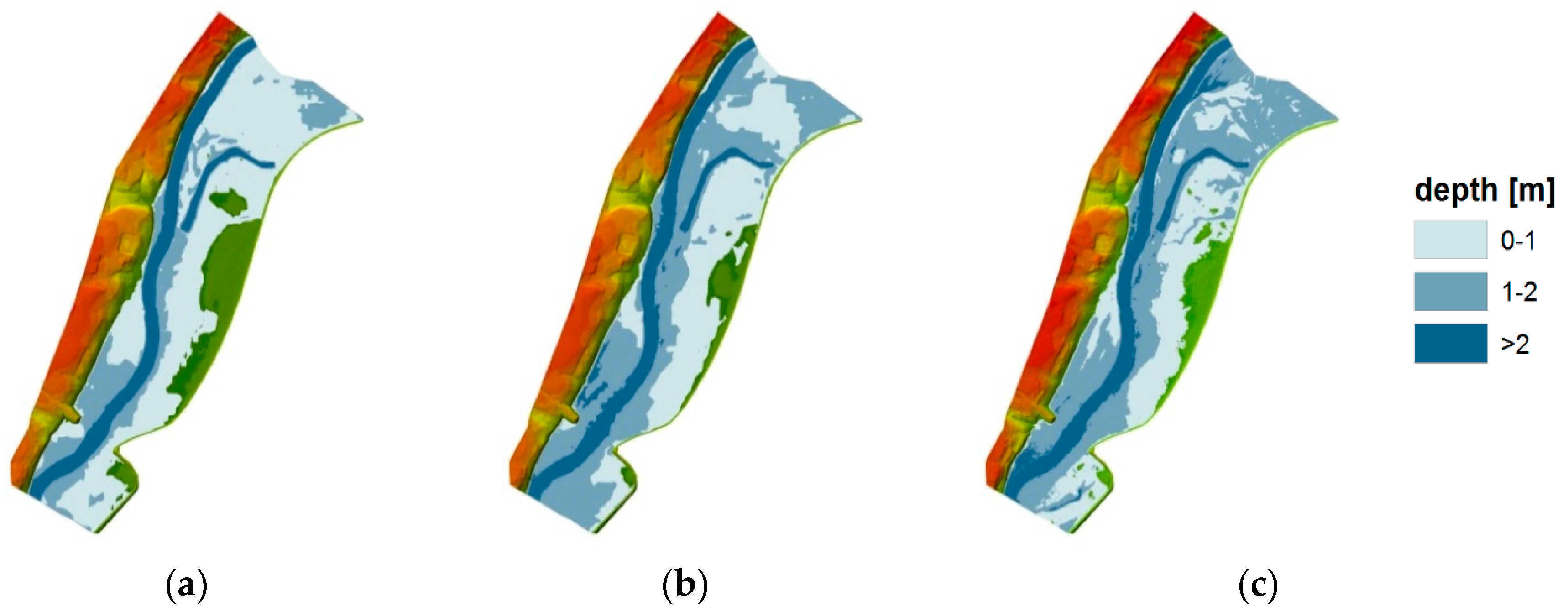
A comparison of the flooded area and the inundation depth values for the flow rate 279.1 m3·s−1 and the corresponding water level at lower boundary equal to 73.82 m a.s.l. is shown in Figure 10. This example was chosen because the flow rate and velocity distribution were measured during the flood in the year 2010 at the cross-section 352.398 using the ADCP StreamPro device (Teledyne RD Instruments, 2008). Measurements of water table elevation at the cross-sections 381.820, 352.170 and 352.398 were also carried out. This additional set of measurement data permitted better assessment of the results obtained from the 2D model.
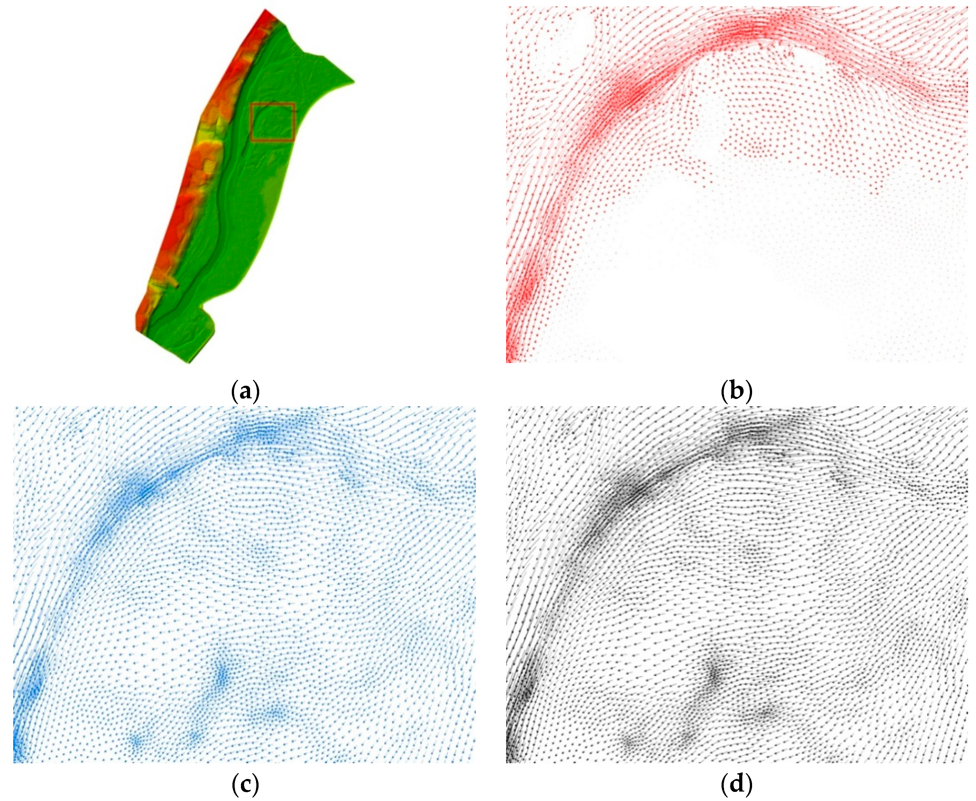
Figure 11 shows a comparison between the velocity vector distributions for the flow rate equal to 279.1 m3·s−1 in a selected sub-area of the area of interest.
Table 3 presents basic statistics of velocity differences between the values obtained from the reference DEM and corrected DEM or original DEM for the flow rate equal to 279.1 m3·s−1. The relations between the flow velocities for the analyzed variants are shown in Figure 12a,b.
A good agreement between the values obtained from corrected DEM and reference DEM can be seen in Figure 12a (the correlation coefficient equal to 0.7915) and in Table 3 (mean value of velocity differences equal to 0.03 m/s). For the original DEM (Figure 12b), both the correlation coefficient (0.6181) and mean value of velocity differences (0.12 m/s) indicate a much lower compliance with reference DEM.
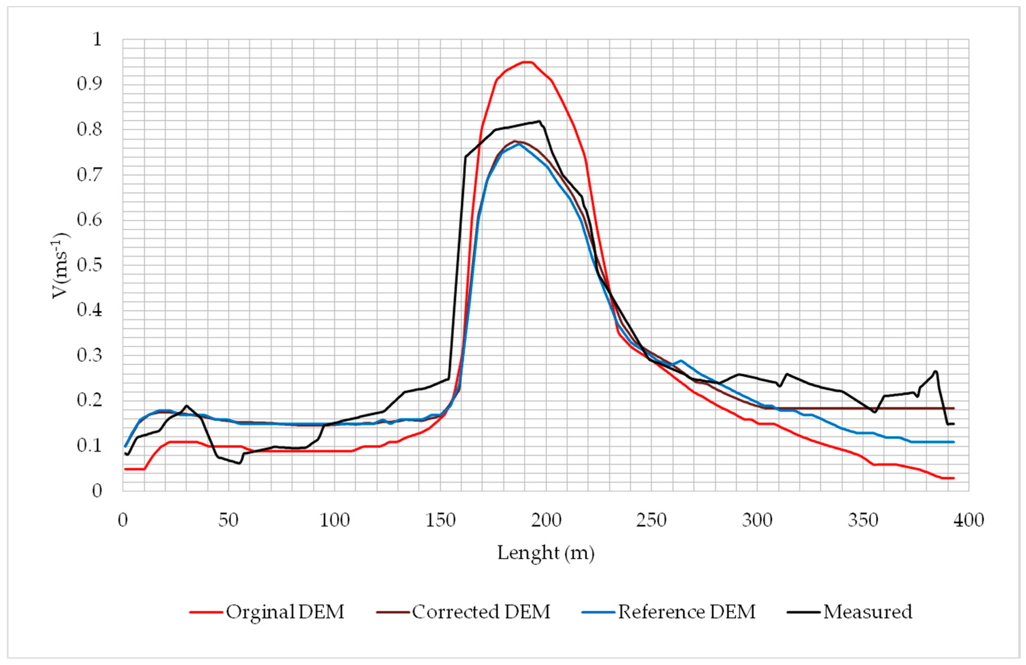
The comparison between the calculated and measured velocity distributions over the length of the cross-section 352.398 is presented in Figure 13. Table 4 shows the basic statistics for this example, i.e., the average flow velocity difference (mean), standard deviation of velocity difference (SD) and correlation coefficient (R) between the values obtained from the 2D model and the measured values.
It should be mentioned that the DEM in which only the FEM mesh was optimized (with no correction of elevations, that is the original DEM) predicts considerably high floodplain elevation values, which of course directly translates to the determined inundation depths and the calculated velocity distributions (see Figure 9, Figure 10 and Figure 11 and Figure 13; Table 2 and Table 3). The maximum difference in volume was more than 28% and more than 50% in inundation area compared with the reference model predictions (reference DEM). This difference also translates, quite significantly, to the velocity distributions in the floodplain and the main channel, as shown in Figure 13. Further, for the example with for the flow rate equal to 279.1 m3·s−1, described in more detail, one may observe that there is a considerable proportion of areas with small modeled velocities, which is clearly a consequence of the small inundation depth. The maximum differences in the determined volume and inundation area between the corrected DEM and reference DEM predictions are distinctly smaller and reach values of 3.86% and 12.39%. Regarding the velocity distributions computed for flow rate equal to 279.1 m3·s−1, there is a very small difference between the corrected DEM and the reference DEM.
Comparison of computed and measured flow velocity distributions along the cross-section 352.398 also confirms better compatibility of the results obtained from 2D model based on the corrected DEM (see Table 4 and Figure 13).
The above analysis confirms that, after an appropriate correction procedure, the corrected model based on poor quality input data is in good quantitative and qualitative agreement with the reference DEM.
3.3. Basic Costs of DEM Correction
The proposed method of preparing data for hydrodynamic models is useful primarily for the areas for which a high-resolution DEM based on LIDAR is not available. It is obvious that the purchase cost of already acquired data is many times lower than the cost of the proposed procedure. It should be noted, however, that the DEM based on LIDAR will gradually become obsolete. Updating the high-resolution DEM will be difficult to carry out in many countries, because of the cost of implementation. Hence, the validation procedure will also concern DEMs currently considered to be accurate and reliable.
The most important cost components are the field measurements and the work associated with the processing of the acquired data using GIS software. A very important component of the cost, which is the measurements of bathymetry, is intentionally omitted in the analysis because regardless of the accuracy of the DEM used, the bathymetry must always be supplemented. The difference in costs will result from the additional work incurred to carry out measurements within the floodplains.
Labor intensity of field measurements depends primarily on the number of measurement points per km2. The number of measurements and their density per km2 can be estimated on the basis of the test measurements performed on the most representative section for the modeled part of the river. Test measurements should have a high density of points per km2. Values of RMSE and SD calculated on the basis of the whole set of measurements will be the reference. In a further step, the value of RMSE and SD for lower density measurements will be calculated by eliminating from the test set every second, third, fourth or fifth point. Such a method of reducing the number of measurements allows preservation of their spatial distribution. In the case of the presented section of the Warta River, it is assumed that the base value will be 400 measurement points per km2. Table 5 shows the value of RMSE and SD for different numbers of field measurements. Obviously, this is largely dependent on the type of terrain and land cover. In this case, we are dealing with a flat terrain covered mostly with grass.
The results presented in Table 5 show that values of RSME and SD do not significantly differ from the reference values (maximum difference for RMSE is 6.4% and 9% for SD) even for a low density of measurements per km2.
The workload of measurements depending on the density per km2 could also be estimated.
The number of measurements per unit of time depends on the density of measurements per km2. With a decrease in the density, the time between measurements is longer, which reduces the number of measurements per unit of time (see Table 6).
The higher the density of measurements per km2, the greater the number of measurements per unit of time. With a decrease in the density, the time between measurements will be longer, which reduces the number of measurements per unit of time (see Table 6). Assuming that the person carrying out the measurements is working effectively for 6 h during the working day and assuming the total cost of one day’s work at the level of 200EUR (the rate for Poland), it is possible to estimate the cost of measurements for 1 km2, which is presented in Table 6. The sum of 200 EUR is the total cost of measurements carried out by a professional geodetic company using the RTK-GPS equipment.
A significant difference in cost of measurements for 1 km2 depending on the density of measurements can be seen. The lowest price for the density of 50 points per km2 is less than 1/3 of the cost of measurements for the density equal to 400 points/km2. The work associated with the processing of the acquired data using GIS software, which is independent of the number of measurements, was estimated at 2 h/km2. For an hourly rate of 25 EUR, it is the amount of 50 EUR/km2. The purchase cost of low-quality DEM based on aerial photographs is about 0.5 EUR/km2. The total cost of the correction of DEM is between 93 EUR/km2 and 184 EUR/km2. For comparison, the price for DEM based on LIDAR developed on request by a specialist company is approximately 320EUR/km2 for the area over 300 km2 (calculated on the basis of analysis of the prices of companies taking part in public tenders in Poland in 2015 and 2016).
The cost analysis indicates that the presented methodology for the correction of low quality DEM may be an alternative for the areas for which there is no available high accuracy DEM. If the analyzed area is from a few to more than a dozen square kilometers, the cost of the DEM based on LIDAR developed on request can be many times higher.
4. Summary and Conclusions
The method for correction of a low quality DEM presented above and based on the poor-quality input data (aerial photography) allows the use of such poor-quality data in the calculation of 2D flows for areas with low-density urban development (e.g., natural river valleys, inter-embankment zones, old river channels). For such areas, the error in the representation of the velocity field will matter less than the retention capacity, which has a significant impact on the transformation of flood waves. The correction of the DEM elevation values is performed following an estimation of the mean error and its sign, as well as following a test for the systematic error based on a series of a small number of direct measurements.
The following conclusions can be formulated.
- -
- The DEMs used for hydraulic modelling, regardless of the declared accuracy, should be verified (if it is possible) on the basis of field measurements
- -
- Analysis of the accuracy of DEM should include autocorrelation analysis of errors, analysis of errors in relation to the structure of land use in the floodplain zone and in relation to the landscape features
- -
- The DEMs should be supplemented with bathymetric data after validation and correction procedures are completed
- -
- In economic terms, for short sections of rivers or small catchments, the use of the corrected DEMs is more reasonable than the DEM based on LiDAR developed on request
The method proposed cannot be applied to urbanized areas; it is suitable only for natural river valleys. As shown in the earlier study [10], the ASTER and STRM models cannot be applied for hydraulic modelling.
Test calculations were performed using a 2D numerical model. These calculations allowed the estimation of the influence of the quality of DEM data on the results obtained from the model. Analysis of the 2D model predictions showed a good agreement between the corrected DEM and reference DEM results. Compliance is present both in terms of accumulated water, the flooded area and velocity field distribution. Furthermore, comparison of the model predictions with field measurements confirmed the reliability of the results.
The most striking difference is that in the volume of accumulated water and the size of inundation area when compared with the reference model, which reach maximum values of 28% and 50%, respectively. This error cannot be compensated by using model calibration procedures based solely on the corrections made to the flow resistance coefficients by adjusting the elevation values in the validation cross-sections. Most importantly, a hydraulic numerical model based on non-corrected low accuracy DEM may produce unrealistic results. Without reliable verification data, this may lead to wrong conclusions in both research and engineering applications.
Acknowledgments
This work is a part of grant from the Polish Ministry of Science and Higher Education (Project No. N N523 744940).
Author Contributions
Ireneusz Laks contributed to data collection, preparation of data for simulations, statistical analysis, preparation of graphs and maps for final presentation of results. Mariusz Sojka was responsible for statistical analysis of collected data, preparation of graphs and maps for final presentation of results. Zbigniew Walczak contributed to data collection, prepared data for numerical analysis and made text formatting for final publication. Rafał Wróżyński contributed to data collection and analysis, preparation of data for simulations, preparation of graphs and maps for final presentation. All co-authors took part in the writing process.
Conflict of Interest
The authors declare no conflict of interest.
References
- Knebl, M.R.; Yang, Z.L.; Hutchison, K.; Maidment, D.R. Regional scale flood modeling using NEXRAD rainfall, GIS, and HEC-HMS/RAS: A case study for the San Antonio River Basin Summer 2002 storm event. J. Environ. Manag. 2005, 75, 325–336. [Google Scholar] [CrossRef] [PubMed]
- Bates, P.D. Integrating remote sensing data with flood inundation models: How far have we got? Hydrol. Processes 2012, 26, 2515–2521. [Google Scholar] [CrossRef]
- Yan, K.; Di Baldassarre, G.; Solomatine, D.P.; Schumann, G.J.P. A review of low-cost space-borne data for flood modelling: Topography, flood extent and water level. Hydrol. Processes 2015, 29, 3368–3387. [Google Scholar] [CrossRef]
- Vaze, J.; Teng, J.; Spencer, G. Impact of DEM accuracy and resolution on topographic indices. Environ. Model. Softw. 2010, 25, 1086–1098. [Google Scholar] [CrossRef]
- Shafique, M.; van der Meijde, M.; Kerle, N.; van der Meer, F. Impact of DEM source and resolution on topographic seismic amplification. Int. J. Appl. Earth Obs. Geoinf. 2011, 13, 420–427. [Google Scholar] [CrossRef]
- Caviedes-Voullième, D.; García-Navarro, P.; Murillo, J. Influence of mesh structure on 2D full shallow water equations and SCS Curve Number simulation of rainfall/runoff events. J. Hydrol. 2012, 448, 39–59. [Google Scholar] [CrossRef]
- Dutta, D.; Herath, S. Effect of DEM Accuracy in Flood Inundation Simulation using Distributed Hydrological Models. Seisan Kenkyu 2001, 53, 602–605. [Google Scholar]
- Yilmaz, M.; Usul, N.; Akyurek, A. Modeling the propagation of DEM uncertainty in flood inundation. In Proceedings of the 24th Annual ESRI International User Conference, San Diego, CA, USA, 9–13 August 2004. [Google Scholar]
- Wechsler, S. Uncertainties associated with digital elevation models for hydrologic applications: A review. Hydrol. Earth Syst. Sci. Discuss. 2007, 11, 1481–1500. [Google Scholar] [CrossRef]
- Walczak, Z.; Sojka, M.; Wróżyński, R.; Laks, I. Estimation of Polder Retention Capacity Based on ASTER, SRTM and LIDAR DEMs: The Case of Majdany Polder (West Poland). Water 2016, 8, 230. [Google Scholar] [CrossRef]
- Merwade, V.; Cook, A.; Coonrod, J. GIS techniques for creating river terrain models for hydrodynamic modeling and flood inundation mapping. Environ. Model. Softw. 2008, 23, 1300–1311. [Google Scholar] [CrossRef]
- Asante, K.O.; Arlan, G.A.; Pervez, S.; Rowland, J. A linear geospatial streamflow modeling system for data sparse environments. Int. J. River Basin Manag. 2008, 6, 233–241. [Google Scholar] [CrossRef]
- Gichamo, T.Z.; Popescu, I.; Jonoski, A.; Solomatine, D. River cross-section extraction from the ASTER global DEM for flood modeling. Environ. Model. Softw. 2012, 31, 37–46. [Google Scholar] [CrossRef]
- Höhle, J.; Höhle, M. Accuracy assessment of digital elevation models by means of robust statistical methods. ISPRS J. Photogramm. Remote Sens. 2009, 64, 398–406. [Google Scholar] [CrossRef]
- Weng, Q. Quantifying uncertainty of digital elevation models derived from topographic maps. In Advances in Spatial Data Handling; SpringerBerlin: Heidelberg, Germany, 2002; pp. 403–418. [Google Scholar]
- Gallay, M.; Lloyd, C.; McKinley, J. Using geographically Weighted regression for analysing elevation error of high-resolution DEMS. In Proceedings of the Ninth International Accuracy Symposium, Leicester, UK, 20–23 July 2010. [Google Scholar]
- Saksena, S.; Merwade, V. Incorporating the effect of DEM resolution and accuracy for improved flood inundation mapping. J. Hydrol. 2015, 530, 180–194. [Google Scholar] [CrossRef]
- Zhou, Q.; Chen, Y. Generalization of DEM for terrain analysis using a compound method. ISPRS J. Photogramm. Remote Sens. 2011, 66, 38–45. [Google Scholar] [CrossRef]
- Karwel, A.K. Estimation of DEM accuracy on the area of Poland based on the elevation data of the LIPS project. Arch. Fotogram. Kartogr. Teledetekcji 2007, 17, 357–362. (In Polish) [Google Scholar]
- Pażus, R.; Osada, E.; Olejnik, S. Levelling geoid 2001. Geodeta Magazyn Geoinformacyjny 2002, 5, 10–17. (In Polish) [Google Scholar]
- Łyszkowicz, A. Geoid in the area of Poland in the author’s investigations. Tech. Sci. 2012, 15, 49–64. [Google Scholar]
- Erdoğan, S. Modelling the spatial distribution of DEM error with geographically weighted regression: An experimental study. Comput. Geosci. 2010, 36, 34–43. [Google Scholar] [CrossRef]
- Anselin, L. GeoDa™ 0.9 User’s Guide. Urbana 2003, 51, 61801. [Google Scholar]
- Taud, H.; Parrot, J.-F.; Alvarez, R. DEM generation by contour line dilation. Comput. Geosci. 1999, 25, 775–783. [Google Scholar] [CrossRef]
- Oky Dicky Ardiansyah, P.; Yokoyama, R. DEM generation method from contour lines based on the steepest slope segment chain and a monotone interpolation function. ISPRS J. Photogramm. Remote Sens. 2002, 57, 86–101. [Google Scholar] [CrossRef]
- Xie, K.; Wu, Y.; Ma, X.; Liu, Y.; Liu, B.; Hessel, R. Using contour lines to generate digital elevation models for steep slope areas: A case study of the Loess Plateau in North China. Catena 2003, 54, 161–171. [Google Scholar] [CrossRef]
- Hashimoto, T. DEM generation from stereo AVNIR images. Adv. Space Res. 2000, 25, 931–936. [Google Scholar] [CrossRef]
- Kornus, W.; Alamús, R.; Ruiz, A.; Talaya, J. DEM generation from SPOT-5 3-fold along track stereoscopic imagery using autocalibration. ISPRS J. Photogramm. Remote Sens. 2006, 60, 147–159. [Google Scholar] [CrossRef]
- Walczak, Z.; Sojka, M.; Laks, I. Assessment of mapping of embankments and control structure on digital elevation model based up on Majdany polder. Annu. Set Environ. Prot. 2013, 15, 2711–2724. [Google Scholar]
- Schröder, P.-M. Zur Numerischen Simulation Turbulenter Freispiegelströmungen Mit Ausgeprägt Dreidimensionaler Charakteristik; Mitteilungen des Instituts für Wasserbau und Wasserwirtschaft der RWTH: Mainz, Germany, 1997. (In Germany) [Google Scholar]
- Sroka, Z.; Walczak, Z.; Wosiewicz, B.J. Analiza Ustalonych Przepływów wód Gruntowych Metodą Elementów Skończonych; Oprogramowanie Inżynierskie; Wydawnictwo Akademii Rolniczej im. Augusta Cieszkowskiego w Poznaniu: Poznań, Poland, 2004. (In Polish) [Google Scholar]
- Suárez, J.P.; Plaza, A. Four-triangles adaptive algorithms for RTIN terrain meshes. Math. Comput. Model. 2009, 49, 1012–1020. [Google Scholar] [CrossRef]
- Anderson, E.S.; Thompson, J.A.; Crouse, D.A.; Austin, R.E. Horizontal resolution and data density effects on remotely sensed LIDAR-based DEM. Geoderma 2006, 132, 406–415. [Google Scholar] [CrossRef]
- Ai, T.; Li, J. A DEM generalization by minor valley branch detection and grid filling. ISPRS J. Photogramm. Remote Sens. 2010, 65, 198–207. [Google Scholar] [CrossRef]
- Horritt, M.S.; Bates, P.D.; Mattinson, M.J. Effects of mesh resolution and topographic representation in 2D finite volume models of shallow water fluvial flow. J. Hydrol. 2006, 329, 306–314. [Google Scholar] [CrossRef]
- Schubert, J.E.; Sanders, B.F.; Smith, M.J.; Wright, N.G. Unstructured mesh generation and landcover-based resistance for hydrodynamic modeling of urban flooding. Adv. Water Resour. 2008, 31, 1603–1621. [Google Scholar] [CrossRef]
- Büttner, O. The influence of topographic and mesh resolution in 2D hydrodynamic modelling for floodplains and Urban areas. Geophys. Res. Abstr. 2007, 9, 08232. [Google Scholar]
- Rismo2D. Finite-Elemente Modellierungsve Rfahren zur 2D-Tiefengemittelten Simulation Stationärer und Instationärer Strömungen. Available online: http://www.hnware.de (accessed on 7 September 2016).
- Wosiewicz, B.; Laks, I.; Sroka, Z. Computer system of flow simulation for the Warta river. In Prace Naukowe Instytutu Geotechniki i Hydromechaniki Politechniki Wrocławskiej, seria Konferencje; Wroclaw University of Technology: Wrocław, Poland, 1996; Volume 38. [Google Scholar]
- Preissmann, A. Propagation of translatory waves in channels and rivers. In Proceedings of the 1st Congress of French Association for Computation, Grenoble, France, 14–16 September 1961; pp. 433–442. [Google Scholar]
Figure 1.
Flowchart for data preparation for 2D hydraulic modeling.

Figure 2.
Study site location.
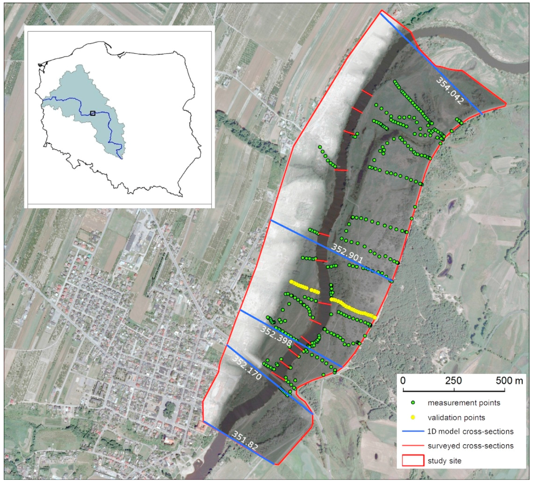
Figure 3.
DEM with the river bathymetry and assignment of the elevation values interpolated from DEM to the nodes of the FEM mesh. (a) Original DEM; (b) main channel river bathymetry interpolation; (c) DEM supplemented with river bathymetry (d) FEM mesh with the elevation interpolated from DEM supplemented with river bathymetry.
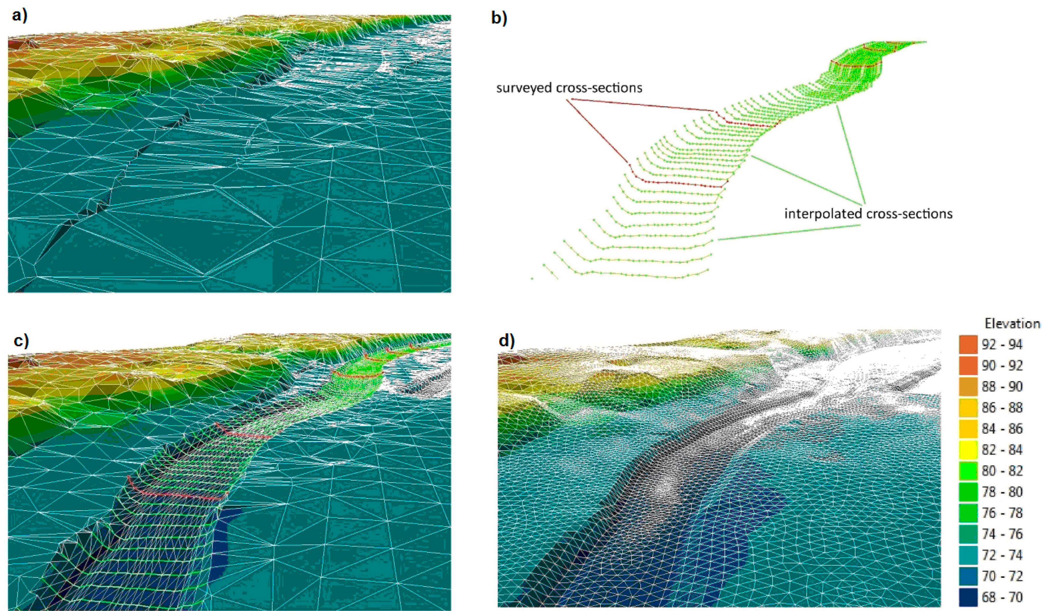
Figure 4.
(a) The calculated and measured water level hydrographs for the flood of 2010 in the section 352.170; and (b) relationship between the water level and flow rate on the basis of the results obtained from the 1D model for the cross-section 351.82.
Figure 4.
(a) The calculated and measured water level hydrographs for the flood of 2010 in the section 352.170; and (b) relationship between the water level and flow rate on the basis of the results obtained from the 1D model for the cross-section 351.82.

Figure 5.
Histogram of the errors ∆h in meters (a); and the normal Q-Q plot for the distribution of errors (b).
Figure 5.
Histogram of the errors ∆h in meters (a); and the normal Q-Q plot for the distribution of errors (b).

Figure 6.
(a) Differences between the reference DEM based on LIDAR data and the original DEM and corrected DEM; (b) distribution of differences between the models.
Figure 6.
(a) Differences between the reference DEM based on LIDAR data and the original DEM and corrected DEM; (b) distribution of differences between the models.

Figure 7.
Relationship between the elevation according to the reference DEM vs. original DEM (a); and from the reference DEM vs. corrected DEM (b).
Figure 7.
Relationship between the elevation according to the reference DEM vs. original DEM (a); and from the reference DEM vs. corrected DEM (b).
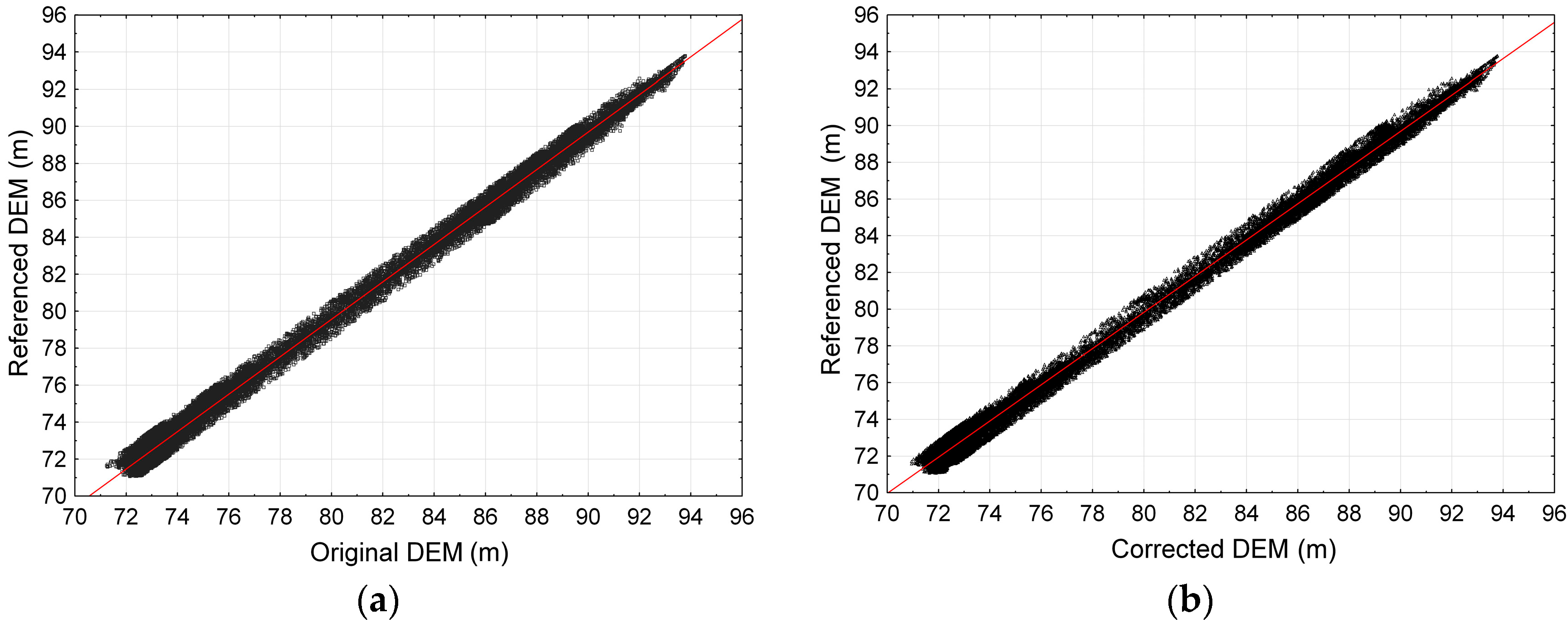
Figure 8.
Comparison of the measured elevation at a selected cross-section with elevation points derived from the original, corrected and referenced DEMs.
Figure 8.
Comparison of the measured elevation at a selected cross-section with elevation points derived from the original, corrected and referenced DEMs.

Figure 9.
Comparison of the curves describing the relationship of the elevation of the water table at the cross-section 351.820 and the volume of accumulated water, calculated on the basis of the results of the 2D model.
Figure 9.
Comparison of the curves describing the relationship of the elevation of the water table at the cross-section 351.820 and the volume of accumulated water, calculated on the basis of the results of the 2D model.

Figure 10.
Comparison of the flooded area and inundation depth values for the flow rate equal to 279.1 m3·s−1: (a) original DEM; (b) corrected DEM; and (c) reference DEM.
Figure 10.
Comparison of the flooded area and inundation depth values for the flow rate equal to 279.1 m3·s−1: (a) original DEM; (b) corrected DEM; and (c) reference DEM.

Figure 11.
Comparison of the velocity distributions obtained from the 2D model for the flow rate equal to 279.1 m3·s−1: (a) DEM with the comparison area marked as the red rectangle; (b) original DEM; (c) corrected DEM; and (d) reference DEM.
Figure 11.
Comparison of the velocity distributions obtained from the 2D model for the flow rate equal to 279.1 m3·s−1: (a) DEM with the comparison area marked as the red rectangle; (b) original DEM; (c) corrected DEM; and (d) reference DEM.

Figure 12.
Relations between the velocity values obtained from the 2D model for the reference DEM and (a) corrected DEM and (b) original DEM. Variants for the flow rate equal to 279.1 m3·s−1.
Figure 12.
Relations between the velocity values obtained from the 2D model for the reference DEM and (a) corrected DEM and (b) original DEM. Variants for the flow rate equal to 279.1 m3·s−1.
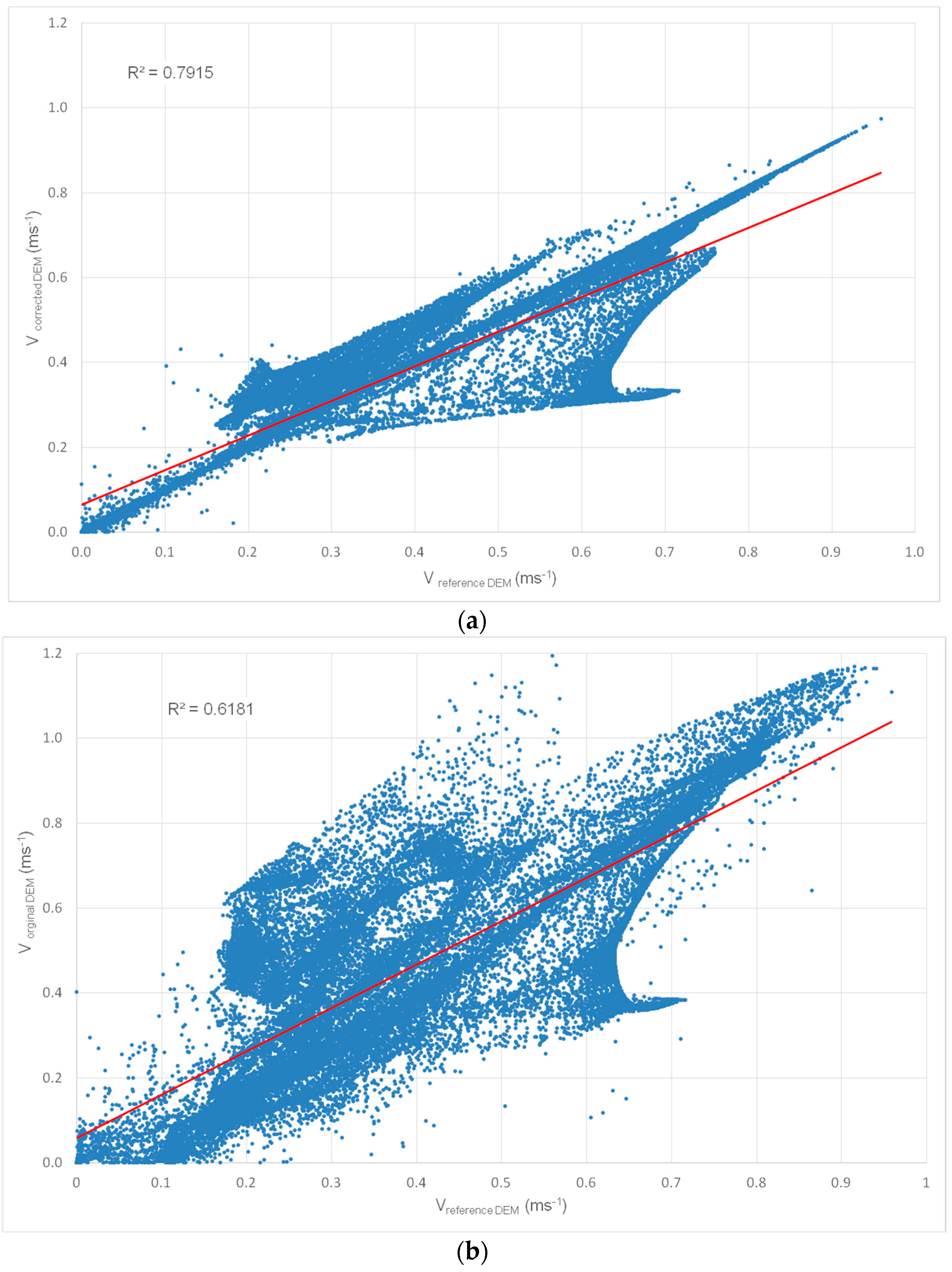
Figure 13.
Distribution of vertical averaged velocity obtained from the 2D model and measured during the flood in year 2010 at the cross-section 352.398.
Figure 13.
Distribution of vertical averaged velocity obtained from the 2D model and measured during the flood in year 2010 at the cross-section 352.398.


Table 1.
Accuracy of DEMs.
| DEM Type | Minimum (m) | Maximum (m) | RMSE (m) | SD (m) | ME (m) |
|---|---|---|---|---|---|
| Original DEM | −0.05 | 1.22 | 0.65 | 0.20 | 0.61 |
| Corrected DEM | −0.31 | 0.72 | 0.21 | 0.17 | 0.13 |
| Reference DEM | −0.50 | 0.63 | 0.35 | 0.16 | 0.12 |
Table 2.
Comparison of the results obtained from 2D model based on various DEMs.
| Water Level m a.s.l. | Flow Rate m3·s−1 | Original DEM | Corrected DEM | Referenced DEM | Original DEM VEE, AEE | Corrected DEM VEE, AEE | |||
|---|---|---|---|---|---|---|---|---|---|
| Volume (m3) | Area (m2) | Volume (m3) | Area (m2) | Volume (m3) | Area (m2) | ||||
| % | % | ||||||||
| 71.6 | 58.2 | 232,060 | 134,512 | 241,863 | 142,480 | 232,865 | 142,036 | VEE = 0.35 AEE = 5.30 | VEE = 3.86 AEE = 0.31 |
| 72 | 77.2 | 301,785 | 145,041 | 325,404 | 211,199 | 316,005 | 210,384 | VEE = 4.50 AEE = 31.06 | VEE = 2.97 AEE = 0.39 |
| 72.4 | 102.4 | 366,208 | 184,934 | 432,995 | 328,972 | 432,270 | 375,480 | VEE = 15.28 AEE = 50.75 | VEE = 0.17 AEE = 12.39 |
| 72.80 | 135.8 | 462,709 | 296,454 | 600,996 | 511,657 | 614,302 | 538,588 | VEE = 24.68 AEE = 44.96 | VEE = 2.17 AEE = 5.00 |
| 73.00 | 156.4 | 529,487 | 380,175 | 712,843 | 606,570 | 730,252 | 619,102 | VEE = 27.49 AEE = 38.59 | VEE = 2.38 AEE = 2.02 |
| 73.30 | 193.3 | 663,362 | 511,717 | 916,696 | 731,603 | 930,610 | 712,951 | VEE = 28.72 AEE = 28.23 | VEE = 1.50 AEE = 2.62 |
| 73.82 | 279.1 | 995,113 | 743,683 | 1,328,694 | 830,030 | 1,332,140 | 817,928 | VEE = 25.30 AEE = 9.08 | VEE = 0.26 AEE = 1.48 |
| 74.20 | 365.1 | 129,4347 | 817,313 | 1,651,892 | 867,727 | 1,650,702 | 855,057 | VEE = 21.59 AEE = 4.41 | VEE = 0.07 AEE = 1.48 |
| 74.60 | 484.3 | 1,631,276 | 863,153 | 2,001,991 | 880,865 | 1,998,564 | 881,538 | VEE = 18.38 AEE = 2.09 | VEE = 0.17 AEE = 0.08 |
| Average Error | VEE = 18.48 AEE = 23.83 | VEE = 1.51 AEE = 2.86 | |||||||
Table 3.
Velocity differences between reference DEM based on LIDAR data and corrected and original DEMs for a flow rate Q = 279.1 m3·s−1.
Table 3.
Velocity differences between reference DEM based on LIDAR data and corrected and original DEMs for a flow rate Q = 279.1 m3·s−1.
| DEM Type | Min | Max | Mean | SD |
|---|---|---|---|---|
| (m·s−1) | (m·s−1) | (m·s−1) | (m·s−1) | |
| corrected DEM | 0.00 | 0.37 | 0.03 | 0.04 |
| original DEM | 0.00 | 0.73 | 0.12 | 0.10 |
Table 4.
Velocity differences between the measured values and those obtained from 2D model based on the reference, corrected and original DEMs for the flow rate Q = 279.1 m3·s−1 at the cross-section 352.398.
Table 4.
Velocity differences between the measured values and those obtained from 2D model based on the reference, corrected and original DEMs for the flow rate Q = 279.1 m3·s−1 at the cross-section 352.398.
| DEM Type | Mean (m·s−1) | SD (m·s−1) | R (‑) |
|---|---|---|---|
| reference DEM | 0.057 | 0.053 | 0.95 |
| corrected DEM | 0.045 | 0.051 | 0.96 |
| original DEM | 0.084 | 0.058 | 0.96 |
Table 5.
RMSE and SD values for the different number of field measurements.
| Points/km2 | RMSE | SD |
|---|---|---|
| 400 | 0.63 | 0.303 |
| 300 | 0.602 | 0.301 |
| 200 | 0.592 | 0.293 |
| 150 | 0.595 | 0.278 |
| 100 | 0.624 | 0.281 |
| 50 | 0.605 | 0.295 |
Table 6.
Costs of measurements.
| Density per 1 km2 | Number of Measurements per Hour | The time for 1 km2 (in Hours) | km2 per Day | Price for 1 km2 (in EUR) |
|---|---|---|---|---|
| 400 | 100 | 4 | 1.5 | 133 |
| 300 | 80 | 3.75 | 1.6 | 125 |
| 200 | 70 | 2.86 | 2.1 | 95 |
| 100 | 60 | 1.67 | 3.6 | 56 |
| 50 | 40 | 1.25 | 4.8 | 42 |
© 2017 by the authors. Licensee MDPI, Basel, Switzerland. This article is an open access article distributed under the terms and conditions of the Creative Commons Attribution (CC BY) license (http://creativecommons.org/licenses/by/4.0/).
Share and Cite
MDPI and ACS Style
Laks, I.; Sojka, M.; Walczak, Z.; Wróżyński, R. Possibilities of Using Low Quality Digital Elevation Models of Floodplains in Hydraulic Numerical Models. Water 2017, 9, 283. https://doi.org/10.3390/w9040283
AMA Style
Laks I, Sojka M, Walczak Z, Wróżyński R. Possibilities of Using Low Quality Digital Elevation Models of Floodplains in Hydraulic Numerical Models. Water. 2017; 9(4):283. https://doi.org/10.3390/w9040283
Chicago/Turabian StyleLaks, Ireneusz, Mariusz Sojka, Zbigniew Walczak, and Rafał Wróżyński. 2017. "Possibilities of Using Low Quality Digital Elevation Models of Floodplains in Hydraulic Numerical Models" Water 9, no. 4: 283. https://doi.org/10.3390/w9040283
Note that from the first issue of 2016, this journal uses article numbers instead of page numbers. See further details here.