
Dynamic Assessment of Comprehensive Water Quality Considering the Release of Sediment Pollution

Institution of water and water environment, Dalian University of Technology, Dalian 116023, China
*
Author to whom correspondence should be addressed.
Water 2017, 9(4), 275; https://doi.org/10.3390/w9040275
Submission received: 16 March 2017
/
Revised: 10 April 2017
/
Accepted: 13 April 2017
/
Published: 15 April 2017
(This article belongs to the Special Issue Water Quality and Health)
Abstract
:Comprehensive assessment of water quality is an important technological measure for water environmental management and protection. Previous assessment methods tend to ignore the influences of sediment pollutant release and dynamic change of the water boundary. In view of this, this paper explores a new method for comprehensive water quality assessment. Laboratory simulation experiments are conducted to analyze the influences of sediment pollutant release on water quality, and the results are taken as increments, coupled with original samples, to constitute a new set of evaluation samples. Dynamic and comprehensive water quality assessment methods are created based on a principal component analysis (PCA)/analytic hierarchy process (AHP)–variable fuzzy pattern recognition (VFPR) model and adopted to evaluate water quality. A geographic information system (GIS) is applied to visually display the results of water quality assessment and the change of the water boundary. This study takes Biliuhe Reservoir as an engineering example. The results show the change process of the water boundary, during which the water level is reduced from 63.10 m to 54.15 m. The reservoir water quality is fine, of which the water quality level (GB3838-2002) is between level 2 and level 3, and closer to level 2 taking no account of sediment pollutant release. The water quality of Biliuhe Reservoir, overall, is worse in summer and better in winter during the monitoring period. Meanwhile, the water quality shows the tendency of being better from upstream to downstream, and the water quality in the surface layer is better than that in the bottom layer. However, water quality is much closer, or even inferior, to level 3 when considering the release of nitrogen and phosphorus in sediments, and up to 42.7% of the original assessment results of the samples undergo changes. It is concluded that the proposed method is comparatively reasonable as it avoids neglecting sediment pollutant release in the water quality assessment, and the presentation of the evaluation results and change of the water boundary is intuitive with the application of GIS.
1. Introduction
Water quality assessment is the foundation of water environmental protection and management [1]. Noteworthy, primary or secondary pollutants in the basin would enter the reservoirs, lakes, rivers, or oceans due to rainfall erosion and river transportation, and then gradually accumulate at the bottom and result in sediment pollution [2]. Sediment pollutants have characteristics of coexistence of aqueous-biological-sedimentary phases [3], and pollutants will release from the sediments under the influence of external conditions, such as dissolved oxygen, hydrodynamics, pH, temperature, and the pollutant concentration in the overlaying water [4,5,6]. In addition, sediment pollution has dual characters of being a source and a sink [7]. In general, the flux direction of liquid pollutants is upward, and the intensity is associated with the concentration of the overlying water [5,8,9], while the flux direction of solid pollutants is the opposite, especially sand, minerals, biological residual bodies, and solid waste [10]. The release of sediment pollutant is a complicated process which is affected by multiple factors which change constantly [11]. Sediment pollutant release is essentially a process where pollutants diffuse from a region with higher concentration to an adjoining region with lower concentration [12]. According to the EPA (1998), 10% of the sediment pollution release could threaten fish, and animals and persons feeding on fish [13]. The nutrients released from sediments in Chaohu Lake in Anhui Province, China, accounts for 21% of exogenous pollutants. Up to 90% of the phosphorus and 80% of the nitrogen accumulates in sediments in the Dianchi Lake in Yunnan Province, China [14]. Reservoirs also face the problem of sediment pollution, such as Yuqiao Reservoir and Xinlicheng Reservoir [15,16]. Thus, sediment pollution is a factor that cannot be ignored in water quality assessment. In addition, the reservoir water level undergoes seasonal and inter-annual fluctuation, which leads to the dynamic change of the water boundary [17]. Thus, the relative positions of water monitoring points change accordingly. A monitoring point that is in the middle level in the vertical direction during flood season may turn into a surface layer in the dry season. The neglect of this change may lead to miscalculations in the water quality assessment. The spatial and temporal variability due to water level fluctuation increases the difficulty of the water quality assessment.
According to the characteristics of uncertainty, randomness, and variability of water quality, researchers have put forward a series of assessment methods, which have been effectively applied in water quality assessments [18,19,20]. Sinha et al. used the comprehensive index method to assess water quality of Hooghly River [21]. Chu et al. explored the use of an artificial neural network to assess water quality [22]. Yan et al. developed a dynamic variable fuzzy set assessment model to judge the water quality [23]. However, the sediment pollution and the water boundary change are ignored. The objectives of this paper are to explore a water quality assessment method that can reflect the influence of sediment pollution and present the evaluation results and water boundary visually.
2. Materials and Methods
2.1. Study Area and Sampling
Biliuhe Reservoir (122°29′24.11″ N; 39°49′12.52″ E) provides up to 80% of the water demand of Dalin City, Northeast China. Biliuhe Reservoir has three main tributaries, including the Biliuhe River, Gelihe River, and Bajiahe River (Figure 1). The watershed area is 2814 km2 and the forest coverage rate is over 80%. The annual rainfall is 742.8 mm, which concentrates in summer (66.9%), and the annual runoff is 6.6 × 10⁸ m3. The maximum water storage of the reservoir is 9.34 × 10⁸ m3. Nitrogen and phosphorus pollution are the main water quality issues of the reservoir. This paper combines the characteristics of the reservoir and the “Specification for Water Environment Monitoring, SL 219-2013” to design a sampling plan.
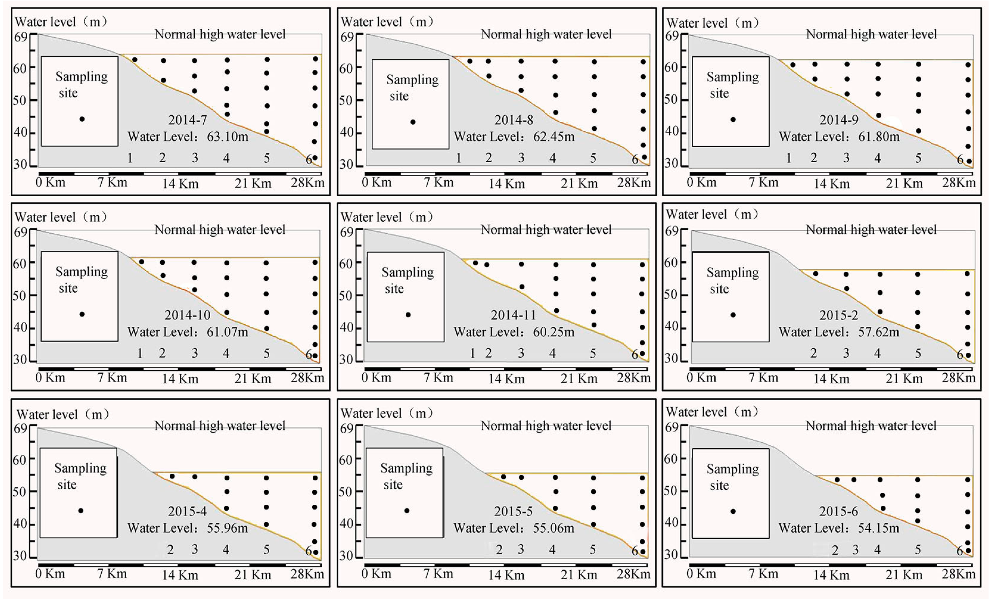
The location map of sampling points is shown in Figure 1 and Figure 2. Samples are collected from July 2014 to June 2015, and December, January, and March belong to the freeze-thawing period which cannot be sampled. In order to simplify the problem, this study considered only the monitoring points in the main stem of Biliuhe Reservoir (Figure 1 and Figure 2). During the monitoring periods, the water level decreases from 63.10 m to 54.15 m and the difference of the water level is 8.95 m. Correspondingly, the water boundary changes. Water samples are collected in accordance with specific conditions: collect one water sample if the water depth is less than 5 m; collect two water samples separately from surface and bottom layer when the depth is between 5 and 10 m; and collect samples every 5 m when the depth is over 10 m. Sediment samples were collected in October 2014, including points 1–6. As the water level fluctuates, the relative positions of the sampling sites change accordingly. To solve this problem, a dynamic sampling method is developed as follows: (1) Cover as many planned sampling sites as possible; (2) add the number of sampling points when the water level is at a high depth; (3) retreat or cancel the relevant sampling points when the water level is at a low depth. A Garmin GPS (GARMIN Corporation, Shengyang, China) is used to mark the sampling point and collect the location information. The water samples are sampled with Niskin bottles (HYDRO-BIOS), the sediment samples are collected by a Van Veen sampler (KC-Denmark). Monitoring indicators of water samples cover dissolved oxygen (DO), total phosphorus (TP), total nitrogen (TN), ammonia nitrogen, chemical oxygen demand (CODMn), pH, iron, and manganese. Monitoring indicators of sediment samples include total nitrogen and total phosphorus. The water samples were carried out in accordance with the “Water and wastewater monitoring and analysis method (Fourth Edition), Beijing: China Environmental Science Press, 2002”. The sediment samples of total nitrogen and total phosphorus were measured by Kjeldahl determination and the Standard measurements and testing (SMT) protocol method [2,5]. The monitoring results were expressed with average values and the errors of the parallel experiments were less than 5%.
2.2. Experiment on Sediment Pollutant Release
This paper studies the release capacity of sediment pollutants under different concentrations of overlying water through a simulation experiment. As eutrophication is the main problem for reservoirs, this paper only considers the release of nitrogen and phosphorus in sediments. Sediment samples are put in a cool and dry place to let them naturally air dry. Then the samples are screened through a 100 mesh sieve (0.15 um) and preserved at −20 °C. Sediment samples (0.2 g each) are placed in a 20 mL centrifuge tube and 20 mL standard solution is added. The phosphorous standard solution of 0, 0.1, 0.2, 1, 2, 4, 6, 10, 15 and 20 mg/L is made by potassium dihydrogen phosphate (KH2PO4, GR) and nitrogen standard solution of 0, 0.1, 0.5, 2, 4, 6, 8, 10, 15 and 20 mg/L is made by potassium nitrate (KNO3,GR). The centrifuge tubes are shaken (180–200 rpm) at an indoor temperature (20 ± 1 °C) for 24 h. After that, samples are then centrifuged (3000 rpm) for 10 min and the filtrates are collected through a 0.45 um fiberglass filter membrane. Next, the sorption-release characters of nitrogen and phosphorus can be calculated by measuring the equilibrium concentration of the collected filtrate. All experiments are carried out in triplicate and averaged, with relative errors less than 5%. Based on the experiment results, the release amount of nitrogen and phosphorus in sediments under different concentrations of each sampling site are calculated [5,6]:
where Ce is the equilibrium concentration, mg/L; C0 is the initial concentration, mg/L; < 0 is the adsorption quantity, mg/kg; > 0 is the release quantity, mg/kg; M is the weight of the sediment, g; V is the volume of adding standard solution, mL.
Furthermore, the amount of sediment release of different initial concentration can calculate by Equation (2) based on the interpolation method:
where is the adsorption/release quantity when the initial concentration is , mg/kg; is the adsorption/release quantity when the initial concentration is , mg/kg; is the adsorption/release quantity when the initial concentration is , mg/kg; the , belong to the standard solution of the experiment and is between and , mg/L.
Next, the water load increment is obtained:
where △x(k) is the increment of the contaminant when the initial concentration is k, mg/L; Q is the sediment content per unit area, g /cm2; < 0 is the adsorption quantity,
> 0 is the release quantity calculated by the interpolation method, mg/kg; and hw is the average water depth, m.
Finally, the new samples are generated:
where Xij is defined as the evaluation characteristic value considering the influence of sediment pollutant release; Xij is the evaluation characteristic value of indicator j and sample i, mg/L; xij is the actual monitoring value of indicator j and sample i, mg/L; △xij is the increment value considering the sediment pollutant release of indicator j and sample i, which is obtained by the laboratory simulation experiment, mg/L.
Xij = xij + △xij
2.3. Dynamic Display of Water Quality Elements (Assessment Results)
To fully understand the situation of water quality, stratified monitoring is normally needed. Reservoir water depth changes dynamically due to rainfall and reservoir operation [24], and the position of sampling sites changes accordingly.
As can be seen in Figure 2, the water level during monitoring period fluctuates between 63.10 m and 54.15 m. Obviously, when the water level is 63.10 m, the distribution of sampling sites is different from that of 54.15 m. Water samples collected at the same depth of the water at different times may belong to different water layers. Geostatistics models in GIS, combined with the image editing capability, can visually export the dynamic status of the topography and the corresponding water quality element data graphically [25,26]. The process is as follows: First, extract the data of the horizontal and vertical topography boundaries of each sampling point based on the topographic data (digital elevation model, DEM). Then, import the position data of the sampling points and corresponding water quality data to the boundary documents. Afterwards, geostatistics is used to conduct the interpolation of water quality elements (assessment results) of the sampling points. Finally, export the water quality distribution diagram of each sampling, respectively, to dynamically and visually display the water quality assessment results. Based on the statistics and pollutant diffusion mechanism, the closer the distance of the points, the more similar the pollutant concentrations and water quality status are. The inverse distance weighting method in GIS is a interpolation method based on the above principles, and the original data will not be changed. Therefore, in this paper, the inverse distance weighting method is selected. Since the interpolation results are used only for display, the interpolation error is not considered in this paper. The detailed steps are as follows:
- (1)
- Generate the DEM map of the study area based on the 1:5000 topographic map
- (2)
- Extract the dynamic boundaries according to the water level
- (3)
- Import the positions of the sampling points
- (4)
- Import the water quality elements (assessment results) of each sample
- (5)
- Generate the distribution of water quality, overall, by the inverse distance weighting method
- (6)
- Export the dynamic distribution diagram of the water quality after inserting a legend
2.4. Assessment Model of Water Quality
The variable fuzzy pattern recognition (VFPR) model has strong adaptability to the dynamic and fuzzification characteristics of water quality assessments, which is applied in various kinds of evaluation issues [27,28]. This paper uses the VFPR model to comprehensively assess water quality.
Assume the set of samples of the water quality is X = (xij), and the set of standards of the water quality is expressed as Y = (), where I = 1, 2, …, m, j = 1, 2, ... , n, h = 1, 2, ... , c. To eliminate the influences of different dimensions and inverse indices, the samples (xij) and standards () are normalized to rij and :
where xij is the value of indicator j of sample i, where i is the number of samples and j is the number of indicators; is the value that defines standard h of indicator j, where h = 1, 2 …, c, c represents the highest level of the standard; rij and are the results of the normalization of the samples (xij) and standards ().
Next, , the synthetic relative membership degree for sample j belonging to standard h, is obtained:
where is the synthetic relative membership degree for sample i belonging to standard h; h is the standard level of water quality; wj is the weight of indicator j; ai is the minimum level of sample i and bi is the maximum level of sample i. a is the optimization criteria parameter, a = 1 (linear), a = 2 (nonlinear); and p is the distance parameter, p = 1 (Hamming distance), p = 2 (Euclidean distance).
When is obtained, the traditional fuzzy assessment model generally takes the maximum membership degree as the final level of the sample, neglecting the information of other membership degrees. This paper regards the level characteristic value as the final assessment result, and the VFPR model considers all possibilities of relevant membership degrees of samples to each standard, which reflects the dynamic change of water quality levels. The model is as follows:
where H is the level characteristic value; and h is the level of standard (h = 1, 2… c).
2.5. Steps of Dynamic Assessment of Comprehensive Water Quality Considering the Release of Sediment Pollution
This paper combines the VFPR model and GIS to dynamically assess water quality and creates a visual display of the results by combining with GIS. The details are as follows:
In the first step, the indicator system of the water quality assessment should be developed on the principles of scientificity, systematicness, feasibility, and practicability.
In the second step, laboratory simulation experiments are conducted to evaluate the influence of sediment release under conditions of different concentrations of the overlying water, so as to obtain water quality assessment samples considering sediment release.
In the third step, Equations (5) and (6) are used to normalize the indicators and standards.
In the fourth step, an appropriate method for weighting indicators should be selected. The common methods are equal weight (EW), principal component analysis (PCA), the analytic hierarchy process (AHP) method, the entropy weight method, and synthetic weight.
In the fifth step, synthetic weight w and the normalization results of rij and are put into Equations (7). Thus, four results of the synthetic relative membership degree uhj are calculated by changing the model parameters (a = 1 or a = 2; p = 1 or p = 2).
In the sixth step, Equation (8) is used to calculate the level characteristic value of the sample i based on the fifth step, and then the average value of the four models is taken as the final assessment result.
In the seventh step, a visible method is applied to visually display the assessment results.
3. Results and Discussion
3.1. Analysis of the Reasonability of Assessment Model
This paper selects eight indicators, i.e., dissolved oxygen (DO, X1), total phosphorus (X2), total nitrogen (X3), ammonia nitrogen (X4), chemical oxygen demand (CODMn, X5), pH (X6), ions (X7), and manganese (X8), to assess water quality. The indicator system covers eutrophication, heavy metal, and comprehensive pollution.
The results of water quality assessment should reflect the actual status of the water quality. To verify the reasonability of the assessment method, eight virtual water quality samples are developed based on the National Surface Water Quality Standard of China (GB3838-2002) and are assessed using different assessment methods and weights.
The created virtual water quality samples can be seen in Table 1. All of the indicator values of sample 1 are better than level 1. Sample 2 is the same as sample 1 except the dissolved oxygen belongs to level 2. Similarly, sample 3 is also the same as sample 1, except the total phosphorus is level 2. Conversely, the indicator values of sample 8 are all worse than level 5, and for samples 4, 5, 6 and 7, the indicator values are just the average values of the neighboring levels from level 1 to level 5, respectively; for example, the indicator values of sample 4 are the average values of level 1 and level 2.
By reference to the literature, this paper uses different methods to determine the weights of indicators which can be seen in Table 2, Table 3 and Table 4, of which the judgment matrix of the analytic hierarchy process (AHP) method is referred to in [28,29,30,31] and the procedure of the PCA method can be seen in [32].
As can be seen in Table 2, the first PC explains 95.829% (>85%) of total variance, and the component matrix of first PC is −0.965X1 + 0.960X2 + 0.994X3 + 0.982X4 + 0.982X5 + 0.980X6 + 0.960X7 + 0.995X8. Next, the normalization method is used to calculate the weight of factors based on the component matrix of the first PC (Table 4).
The Table 3 shows the judgment matrix of the AHP, and then the eigenvector of the largest eigenvalue could be used to calculate the weight of factors by the normalization method (Table 4).
Obviously, different methods determine the weights of the indicators from different aspects. Appropriate weights can be determined by comparison and optimization.
Then the virtual samples are assessed with different methods and different weights, and the assessment results can be seen in Table 5. WQI is a comprehensive index method based on equal weight, EW-VFPR is a variable fuzzy pattern recognition (VFPR) model based on equal weight. AHP-VFPR is a VFPR model based on the analytic hierarchy process (AHP) weight. PCA-VFPR is a VFPR model based on principal component analysis (PCA) weighting. PCA/AHP-VFPR is a VFPR model based on the synthesis weight of PCA and AHP. PCA/AHP-FCA is a fuzzy synthetic evaluation [33] (FCA) model based on the synthesis weight of PCA and AHP. I-PCA/AHP-FCA is an improved FCA model using Equation (4), based on the synthesis weight of PCA and AHP. As is shown in Table 3, the assessment results of the WQI method and PCA/AHP-FCA method are inattentive with the actual situation, because some indicators in samples 2 and 3 are actually inferior to level 1. The WQI method is based on equal weight, so it considers all other indicators’ indices and weakens each single indicator’s impact, which leads to unsatisfactory results; the PCA/AHP-FCA method determines the result according to the maximum membership degree selection principle, which neglects the information of other membership degrees and, finally, results in inaccuracy to some extent. For example, the membership degree of sample 3 is 0.8 to level 1 and 0.2 to level 2. However, according to the maximum membership degree selection principle, the result of sample 3 is level 1, which neglects the information of level 2. The assessment result of VFPR model based on the synthesis weight is in accordance with the actual case. The model is able to reflect the variability of the indicators when the indicators are changed. Previous studies show that the synthesis weight not only includes the information of the original data, but includes the researchers’ knowledge about specific problems, which makes the results more reliable. The assessment result of the I-PCA/AHP-FCA method is similar to the PCA/AHP-VFPR method, but the I-PCA/AHP-FCA method would lose some information of the comprehensive samples.
Above all, the PCA/AHP-VFPR model considers the successive information of relevant membership degrees of each single indicator to the water standard, and the successive information of the relevant membership degrees of the comprehensive water quality to water levels. The PCA/AHP-VFPR model is a dynamic and fuzzy method, which is in line with the water quality properties, so it is appropriate for dynamic assessment of the comprehensive water quality.
3.2. Analysis of Release Ability of Nitrogen and Phosphorus in Sediment
To simplify, temporal variation of sediment and complicated changes of hydraulics are not considered. According to the field investigation of Biliuhe Reservoir, the average deposit depth is 40 centimeters, the dry soil density is 1.55 g/cm3, and the sediment moisture content measured is about 45.5%. Based on the results above, the sediment content of per unit area (Q) is calculated to be 34.4 g/cm2. Given that the average water depth (hw) of Biliuhe Reservoir is 12.8 m, by inputting the release amount () (mg/kg) of each point into the calculation equation we can obtain the increment of the sediment release into the water. Further, the amount of sediment release and water load increment is calculated by Equations (1)–(4). Adding the water load increment to the original monitoring data creates new water quality data that considers the sediment release. When those above data are introduced into the assessment model, the assessment result of the comprehensive water quality considering the release of sediment pollution is acquired.
For simplification, we take the average concentration of nitrogen and phosphorus of the monitoring points during monitoring period as the concentration in the overlaying water, i.e., the concentration of nitrogen and phosphorus in the overlaying water is 2.29 mg/L and 0.027 mg/L separately. Then the release amount () of the sites are calculated by Equation (2). Based on the above-mentioned data, the increment of nitrogen and phosphorus of each monitoring point is obtained, which can be seen in Table 6.
Table 6 shows the release ability of nitrogen and phosphorus in sediment is greater under shaking, leading to an increase of the water pollution load. It must be declared that the shaking in the experiment does not agree with the actual water environment, and the influence of the solid matter’s settlement is not considered, either. However, the result could be regarded as the potential release ability of nitrogen and phosphorus in the sediment, and is still valuable in analyzing the influences of sediment release on water quality assessment, indeed.
This paper adds the increment of total nitrogen and total phosphorus with the corresponding original data to obtain new evaluation samples, and then analyzes the water quality comprehensive status, considering the influences of sediment release.
3.3. Results of Comprehensive Water Quality Assessment
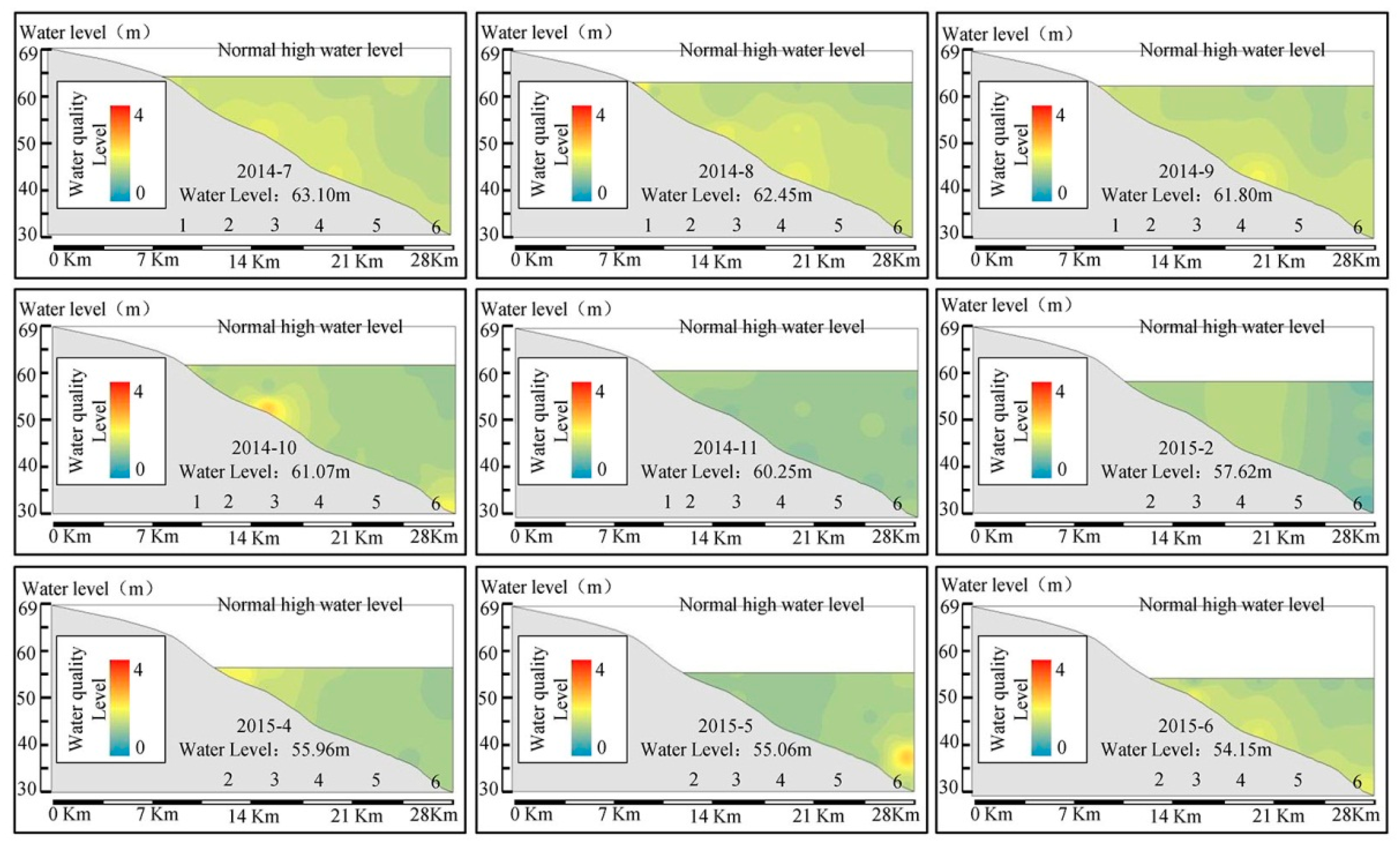
We input the original monitoring samples into the assessment model, and use GIS to export the dynamic assessment results, which are shown in Figure 3. The comprehensive water quality index varies from 1.97 to 3.03. The average water quality index is 2.36 and the variable coefficient is 7.15.
It can be easily seen in Figure 3 that the water level is reduced from 63.10 m to 54.15 m and the water boundary is clear. The water quality is fine (2.36), overall, and worse in summer and better in winter, overall. The monthly average water quality level in July, August, and September in 2014 are 2.39, 2.35 and 2.37, respectively. The monthly average water quality level in February in 2015 is 2.27. The change of the comprehensive water quality level is in accordance with the actual reservoir environmental change. During summer, heavy rainfall would import a large amount of pollutants, which decrease the water quality. Meanwhile, the thermocline would impede the dissolved oxygen exchange, which contributes to the anaerobic environment at the bottom and sediment pollution release [34,35]. In winter, small amounts of runoff carry relatively fewer pollutants into the reservoir, which is in quiescent state, overall, and low temperature can also promote the increase of dissolved oxygen [36]. Meanwhile, the water quality shows the tendency of becoming better from upstream to downstream (dam) where the average level of the water quality is 2.31, and is better than others. The process of hydraulic transport agrees with this trend [37]. The water quality in the surface layer is better than that in the bottom layer because of sediment pollution, which influences water quality by releasing contaminants and consuming dissolved oxygen [38]. The comprehensive water quality indices in the surface layer of Points 3–6 are 2.34, 2.33, 2.27 and 2.27, respectively, while in the bottom layer the indices are 2.62, 2.63, 2.42 and 2.42. This case also occurred in July 2014, September 2014, and June 2015, which are mainly in relation with the change of dissolved oxygen. Thus, the influence of sediment pollution should be considered in the water quality assessment.
3.4. Assessment Results of Comprehensive Water Quality Considering Release of Sediment Pollution
We input the evaluation samples considering sediment release into the assessment model, and use GIS to export the dynamic assessment results.
By comparing Figure 3 and Figure 4, we can find that the average assessment results considering the release of nitrogen and phosphorus in sediment is 3.03 and the variable coefficient is 3.60. The comprehensive water quality level significantly declines. The comprehensive water quality level of 42.7% of the sampling points descends to levels inferior to level 3, which means the results of the assessment also change. Therefore, sediment pollution release can significantly change the status of water quality. Actually, sediment pollutants have dual characters of being sources and sinks of pollutants and change with external conditions [10]. Thus, it is necessary to combine the actual external conditions with the water quality comprehensive assessment to accurately assess the water quality status in the next.
4. Conclusions
This paper analyzes the influence of the release of nitrogen and phosphorus in sediments on water quality through a physical simulation experiment, and explores a method to dynamically assess comprehensive water quality based on the PCA/AHP-VFPR model. GIS is applied to visually display the assessment results of water quality and reflect the change of the water boundary. Taking Biliuhe Reservoir as an example, the results show that the water quality is good, which is between level 2 and level 3, and much closer to level 2; the water boundary can also be visual demonstrated, in which the water level is reduced from 63.10 m to 54.15 m. The water quality of Biliuhe Reservoir, overall, is worse in summer and better in winter during the monitoring period. Meanwhile, water quality shows the tendency of becoming better from the entrance to the dam site, and the water quality in the surface layer is better than that in the bottom layer. The release of nitrogen and phosphorus in sediments could prominently affect water quality. Water quality is closer to, or worse than, level 3 considering the effects, and 42.7% of the samples are changed to being inferior to level 3.
This paper preliminarily studies the influence of sediment release on water quality assessment, but the effects of the microenvironment in water are ignored, which requires further study. This paper believes that the proposed method contributes to the study of the dynamic change of water quality, and it could also provide a reference for water resource protection and similar studies.
Acknowledgments
The authors would like to thank the anonymous reviewers. This work was supported by the National Natural Science Foundation of China (No. 51327004; No. 51279022; No. 51679026), the project of the comprehensive investigation of water quality in Biliuhe Reservoir, and the National Key Research and Development Program of China (2016YFC0400903). The datasets are provided by the Biliuhe Reservoir Management Bureau of Dalian.
Author Contributions
Tianxiang Wang and Shiguo Xu conceived and designed the experiments; Tianxiang Wang performed the experiments; Jianwei Liu and Shiguo Xu analyzed the data; Shiguo Xu contributed reagents/materials/analysis tools; and Tianxiang Wang wrote the paper.
Conflicts of Interest
The authors declare no conflict of interest.
References
- Tan, X.; Sheldon, F.; Bunn, S.E.; Zhang, Q.F. Using diatom indices for water quality assessment in a subtropical river, China. Environ. Sci. Pollut. Res. 2013, 20, 4164–4175. [Google Scholar] [CrossRef] [PubMed]
- Xu, S.G.; Wang, T.X. Review of research on accumulation process and effect of internal pollution of reservoir. Adv. Sci. Technol. Water Resour. 2015, 35, 162–167. (In Chinese) [Google Scholar] [CrossRef]
- Jin, X.C.; Wang, S.R.; Jiang, X. Preliminary study of the three dimension model of the lake water sediment interface. Res. Environ. Sci. 2004, 17, 1–6. (In Chinese) [Google Scholar]
- Cheng, H.M.; Hua, Z.L. Effects of hydrodynamic disturbances and resuspension characteristics on the release of tetrabromobisphenol A from sediment. Environ. Pollut. 2016, 219, 785–793. [Google Scholar] [CrossRef] [PubMed]
- Zhang, Y.; He, F.; Liu, Z.S.; Liu, B.Y.; Zhou, Q.H.; Wu, Z.B. Release characteristics of sediment phosphorus in all fractions of West Lake, Hang Zhou, China. Ecol. Eng. 2016, 95, 645–651. [Google Scholar] [CrossRef]
- Puttonen, I.; Kohonen, T.; Mattila, J. Factors controlling phosphorus release from sediments in coastal archipelago areas. Mar. Pollut. Bull. 2016, 108, 77–86. [Google Scholar] [CrossRef] [PubMed]
- Hongthanat, N.; Kovar, J.L.; Thompson, M.L. Phosphorus source-sink relationships of stream sediments in the Rathbun Lake watershed in southern Iowa, USA. Environ Monit. Assess. 2016, 188, 453. [Google Scholar] [CrossRef] [PubMed]
- Wang, H.; Zhou, Y.Y.; Wang, X. Transport dynamics of Cr and Zn between deposited sediment and overlying water. Clean Soil Air Water 2016, 44, 1453–1460. [Google Scholar] [CrossRef]
- Yang, Q.Z.; Zhao, H.Z.; Zhao, N.N.; Ni, J.R.; Gu, X.J. Enhanced phosphorus flux from overlying water to sediment in a bioelectrochemical system. Bioresour. Technol. 2016, 216, 182–187. [Google Scholar] [CrossRef] [PubMed]
- Wang, H.; Zhao, Y.J.; Wang, X.; Liang, D.F. Fluctuations in Cd release from surface-deposited sediment in a river-connected lake following dredging. J. Geochem. Explor. 2017, 172, 184–194. [Google Scholar] [CrossRef]
- Wu, Y.H.; Wen, Y.J.; Zhou, J.X. Phosphorus Release from Lake Sediments: Effects of pH, Temperature and Dissolved Oxygen. Ksce J. Civ. Eng. 2014, 18, 323–329. [Google Scholar] [CrossRef]
- Liu, C.; Zhong, J.C.; Wang, J.J.; Zhang, L.; Fan, C.X. Fifteen-year study of environmental dredging effect on variation of nitrogen and phosphorus exchange across the sediment-water interface of an urban lake. Environ. Pollut. 2016, 219, 639–648. [Google Scholar] [CrossRef] [PubMed]
- National Service Center for Environmental Publications (USEPA). EPA’s Contaminated Sediment Management Strategy; National Service Center for Environmental Publications: Washington, DC, USA, 1998.
- Zhang, X.H. Water Environment Restoration Engineering Principle and Its Application; Chemical Industry Press: Beijing, China, 2002. (In Chinese) [Google Scholar]
- Wu, G.D.; Wei, Z.; Su, R.X. Distribution, accumulation and mobility of mercury in superficial sediment samples from Tianjin, northern China. J. Environ. Monitor. 2011, 13, 2488–2495. [Google Scholar] [CrossRef] [PubMed]
- Zheng, B.H.; Qin, Y.W.; Zhang, L.; Ma, Y.Q.; Zhao, Y.M.; Wen, Q. Sixty-year sedimentary records of polymetallic contamination (Cu, Zn, Cd, Pb, As) in the Dahuofang Reservoir in Northeast China. Environ. Earth Sci. 2016, 75, 486. [Google Scholar] [CrossRef]
- Ji, D.B.; Wells, S.A.; Yang, Z.J.; Liu, D.F.; Huang, Y.L.; Ma, J.; Berger, C.J. Impacts of water level rise on algal bloom prevention in the tributary of Three Gorges Reservoir, China. Ecol. Eng. 2017, 98, 70–81. [Google Scholar] [CrossRef]
- Lamastra, L.; Balderacchi, M.; Di, G.A.; Monchiero, M.; Trevisan, M. A novel fuzzy expert system to assess the sustainability of the viticulture at the wine-estate scale. Sci. Total Environ. 2016, 572, 724–733. [Google Scholar] [CrossRef] [PubMed]
- He, T.; Zhang, L.G.; Zeng, Y.; Zuo, C.Y.; Li, J. Water Quality Comprehensive Index Method of Eltrix River in Xin Jiang Province using SPSS. Procedia Earth Plantetary Sci. 2012, 5, 314–321. [Google Scholar] [CrossRef]
- Lopez-Doval, J.C.; Montagner, C.C.; de Alburquerque, A.F.; Moschini-Carlos, V.; Umbuzeiro, G.; Pompeo, M. Nutrients, emerging pollutants and pesticides in a tropical urban reservoir: Spatial distributions and risk assessment. Sci. Total Environ. 2017, 575, 1307–1324. [Google Scholar] [CrossRef] [PubMed]
- Sinha, K.; Das, P. Assessment of water quality index using cluster analysis and artificial neural network modeling: A case study of Hooghly river basin, west Bengal, India. Desalin. Water Treat. 2015, 54, 28–36. [Google Scholar] [CrossRef]
- Chu, H.B.; Lu, W.X.; Zhang, L. Application of artificial neural network in environmental water quality assessment. J. Agric. Sci. Technol. 2013, 2, 343–356. [Google Scholar]
- Yan, F.; Liu, L.; Zhang, Y.; Chen, M.S.; Chen, N. The research of dynamic variable fuzzy set assessment model in water quality evaluation. Water Resour. Manag. 2016, 30, 63–78. [Google Scholar] [CrossRef]
- Logez, M.; Roy, R.; Tissot, L.; Argillier, C. Effects of water-level fluctuations on the environmental characteristics and fish-environment relationships in the littoral zone of a reservoir. Fund. Appl. Limnol. 2016, 189, 37–49. [Google Scholar] [CrossRef]
- Easton, Z.M. Defining Spatial Heterogeneity of Hillslope Infiltration Characteristics Using Geostatistics, Error Modeling, and Autocorrelation Analysis. J. Irrig. Drain-ASCE 2013, 139, 718–727. [Google Scholar] [CrossRef]
- Deshmukh, K.K.; Aher, S.P. Assessment of the Impact of Municipal Solid Waste on Groundwater Quality near the Sangamner City using GIS Approach. Water Resour. Manag. 2016, 30, 2425–2443. [Google Scholar] [CrossRef]
- Peng, H.; Zhou, H.C.; Li, M. Assessing water renewal of the northern coastal zone in China using a variable fuzzy pattern recognition model. J. Hydroinform. 2010, 12, 339–350. [Google Scholar] [CrossRef]
- Xu, S.G.; Wang, T.X.; Hu, S.D. Dynamic Assessment of Water Quality Based on a Variable Fuzzy Pattern Recognition Model. Int. J. Environ. Res. Public Health 2015, 12, 2230–2248. [Google Scholar] [CrossRef] [PubMed]
- Chakraborty, S.; Kumar, R.N. Assessment of groundwater quality at a MSW landfill site using standard and AHP based water quality index: A case study from Ranchi, Jharkhand, India. Environ. Monit. Assess. 2016, 188, 335. [Google Scholar] [CrossRef] [PubMed]
- Bozdag, A. Combining AHP with GIS for assessment of irrigation water quality in Cumra irrigation district (Konya), Central Anatolia, Turkey. Environ. Earth Sci. 2015, 73, 8217–8236. [Google Scholar] [CrossRef]
- Ou, C.P.; St-Hilaire, A.; Ouarda, T.B.M.J.; Conly, F.M.; Armstrong, N.; Khalil, B.; Proulx-Mclnnis, S. Coupling geostatistical approaches with PCA and fuzzy optimal model (FOM) for the integrated assessment of sampling locations of water quality monitoring networks (WQMNs). J. Environ. Monit. 2012, 14, 3118–3128. [Google Scholar] [CrossRef] [PubMed]
- Dalal, S.G.; Shirodkar, P.V.; Jagtap, T.G.; Naik, B.G.; Rao, G.S. Evaluation of significant sources influencing the variation of water quality of Kandla creek, Gulf of Katchchh, using PCA. Environ. Monit. Assess. 2010, 163, 49–56. [Google Scholar] [CrossRef] [PubMed]
- Lu, X.W.; Li, L.Y.; Lei, K.; Wang, L.J.; Zhai, Y.X.; Zhai, M. Water quality assessment of Wei River, China using fuzzy synthetic evaluation. Environ. Earth Sci. 2010, 60, 1693–1699. [Google Scholar] [CrossRef]
- Flores, P.E.D.; Geronimo, F.K.F.; Alihan, J.C.P.; Kim, L.H. Transport of nonpoint source pollutants and stormwater runoff in a hybrid rain garden system. J. Wetl. Res. 2016, 18, 481–487. [Google Scholar] [CrossRef]
- Nemirovskaya, I.A. Variations in different compounds in Volga water, suspension, and bottom sediments in the summer of 2009. Water Resour. 2012, 39, 533–545. [Google Scholar] [CrossRef]
- Stefanovic, D.L.; Stefan, H.G. Two-dimensional temperature and dissolved oxygen dynamics in the littoral region of an ice-covered lake. Cold Reg. Sci. Technol. 2002, 34, 159–178. [Google Scholar] [CrossRef]
- Reagan, M.T.; Moridis, G.J.; Keen, N.D.; Johnson, J.N. Numerical simulation of the environmental impact of hydraulic fracturing of tight/shale gas reservoirs on near-surface groundwater: Background, base cases, shallow reservoirs, short-term gas, and water transport. Water Resour. Res. 2015, 51, 2543–2573. [Google Scholar] [CrossRef] [PubMed]
- Doig, L.E.; North, R.L.; Hudson, J.J.; Hewlett, C.; Lindenschmidt, K.E.; Liber, K. Phosphorus release from sediments in a river-valley reservoir in the northern Great Plains of North America. Hydrobiologia 2017, 787, 323–339. [Google Scholar] [CrossRef]
Figure 1.
The horizontal sampling point map of Biliuhe Reservoir.
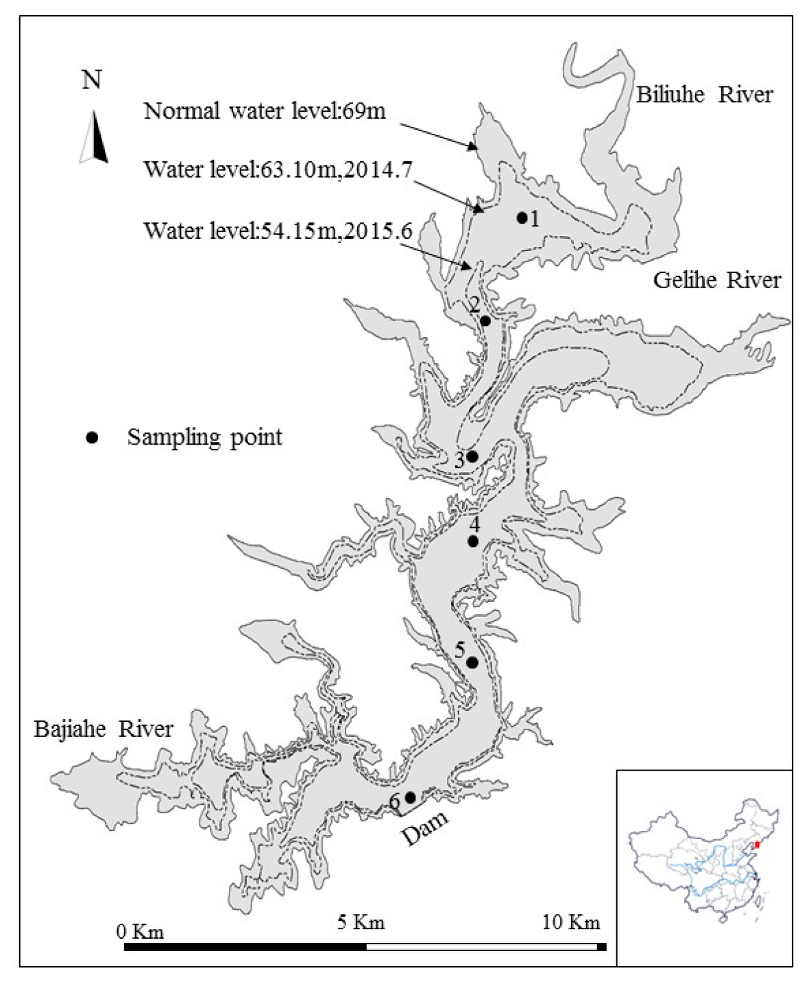
Figure 2.
The vertical sampling points map in Biliuhe reservoir.

Figure 3.
The vertical change of water quality of Biliuhe Reservoir.

Figure 4.
The vertical change of comprehensive water quality considering sediment release of Biliuhe Reservoir.
Figure 4.
The vertical change of comprehensive water quality considering sediment release of Biliuhe Reservoir.


Table 1.
Virtual samples and water quality standards (GB3838-2002).
| Indicators | |||||||||
|---|---|---|---|---|---|---|---|---|---|
| X1 (mg/L) | X2 (mg/L) | X3 (mg/L) | X4 (mg/L) | X5 (mg/L) | X6 (-) | X7 (mg/L) | X8 (mg/L) | ||
| Virtual water samples | 1 | 7.6 | 0.005 | 0.1 | 0.1 | 1 | 7 | 0.05 | 0.005 |
| 2 | 6.2 | 0.005 | 0.1 | 0.1 | 1 | 7 | 0.05 | 0.005 | |
| 3 | 7.6 | 0.02 | 0.1 | 0.1 | 1 | 7 | 0.05 | 0.005 | |
| 4 | 6.75 | 0.0175 | 0.35 | 0.325 | 3 | 7.5 | 0.15 | 0.03 | |
| 5 | 5.5 | 0.0375 | 0.75 | 0.75 | 5 | 8.5 | 0.25 | 0.075 | |
| 6 | 4 | 0.075 | 1.25 | 1.25 | 8 | 9.5 | 0.4 | 0.15 | |
| 7 | 2.5 | 0.15 | 1.75 | 1.75 | 12.5 | 12 | 0.75 | 0.3 | |
| 8 | 1 | 0.4 | 3 | 3 | 16 | 14 | 2 | 0.5 | |
| Water quality standards | 1 | 7.5 | 0.01 | 0.2 | 0.15 | 2 | 6–9 | <0.3 | <0.1 |
| 2 | 6 | 0.025 | 0.5 | 0.5 | 4 | ||||
| 3 | 5 | 0.05 | 1 | 1 | 6 | ||||
| 4 | 3 | 0.1 | 1.5 | 1.5 | 10 | >9 or <6 | >0.3 | >0.1 | |
| 5 | 2 | 0.2 | 2 | 2 | 15 | ||||
Table 2.
The eigenvalues and contribution rates of PCA.
| Component | Initial Eigenvalues | ||
|---|---|---|---|
| Total | % of Variance | Cumulative % | |
| 1 | 7.666 | 95.829 | 95.829 |
| 2 | 0.248 | 3.101 | 98.930 |
| 3 | 0.063 | 0.790 | 99.721 |
| 4 | 0.017 | 0.206 | 99.927 |
| 5 | 0.003 | 0.043 | 99.970 |
| 6 | 0.002 | 0.026 | 99.996 |
| 7 | 0.000 | 0.003 | 99.999 |
| 8 | 4.423 × 10⁻⁵ | 0.001 | 100.000 |
Table 3.
The judgment matrix of AHP.
| Judgment Matrix | ||||||||
|---|---|---|---|---|---|---|---|---|
| X1 | X2 | X3 | X4 | X5 | X6 | X7 | X8 | |
| X1 | 1 | 1 | 2 | 4 | 4 | 4 | 3 | 3 |
| X2 | 1 | 1 | 2 | 4 | 4 | 4 | 3 | 3 |
| X3 | 0.5 | 0.5 | 1 | 2 | 2 | 2 | 2 | 2 |
| X4 | 0.25 | 0.25 | 0.5 | 1 | 1 | 1 | 0.5 | 0.5 |
| X5 | 0.25 | 0.25 | 0.5 | 1 | 1 | 1 | 0.5 | 0.5 |
| X6 | 0.25 | 0.25 | 0.5 | 1 | 1 | 1 | 0.5 | 0.5 |
| X7 | 0.33 | 0.33 | 0.5 | 2 | 2 | 2 | 1 | 1 |
| X8 | 0.33 | 0.33 | 0.5 | 2 | 2 | 2 | 1 | 1 |
| The consistency ratio is 0.0078 < 0.1 | ||||||||
Table 4.
Weights of indicators determined by different methods.
| Serial Number | Indicators | Weight | |||
|---|---|---|---|---|---|
| AHP | PCA | AHP-PCA | EW | ||
| 1 | DO, X1 | 0.251 | 0.124 | 0.249 | 0.125 |
| 2 | Total phosphorus, X2 | 0.251 | 0.123 | 0.247 | 0.125 |
| 3 | Total nitrogen, X3 | 0.137 | 0.127 | 0.140 | 0.125 |
| 4 | Ammonia nitrogen, X4 | 0.057 | 0.127 | 0.058 | 0.125 |
| 5 | CODMn, X5 | 0.057 | 0.125 | 0.057 | 0.125 |
| 6 | Ph, X6 | 0.057 | 0.125 | 0.057 | 0.125 |
| 7 | Iron, X7 | 0.095 | 0.123 | 0.094 | 0.125 |
| 8 | Manganese, X8 | 0.095 | 0.127 | 0.097 | 0.125 |
Table 5.
Assessment results of different methods.
| Samples | Methods | ||||||
|---|---|---|---|---|---|---|---|
| WQI | EW-VFPR | PCA-VFPR | AHP-VFPR | PCA/AHP-VFPR | I-PCA/AHP-FCA | PCA/AHP-FCA | |
| 1 | 1.00 | 1.00 | 1.00 | 1.00 | 1.00 | 1.00 | 1.00 |
| 2 | 1.00 | 1.23 | 1.22 | 1.49 | 1.48 | 1.21 | 1.00 |
| 3 | 1.00 | 1.05 | 1.04 | 1.08 | 1.07 | 1.16 | 1.00 |
| 4 | 2.00 | 1.50 | 1.50 | 1.50 | 1.50 | 1.50 | 1~2 |
| 5 | 3.00 | 2.50 | 2.50 | 2.50 | 2.50 | 2.50 | 2~3 |
| 6 | 4.00 | 3.50 | 3.50 | 3.50 | 3.50 | 3.50 | 3~4 |
| 7 | 5.00 | 4.50 | 4.50 | 4.50 | 4.50 | 4.50 | 4~5 |
| 8 | 5.00 | 5.00 | 5.00 | 5.00 | 5.00 | 5.00 | 5.00 |
Table 6.
The increment of sediment release on water quality.
| Sampling Sites | TN | TP | ||
|---|---|---|---|---|
| Q (mg/kg) | △x (mg/L) | Q (mg/kg) | △x (mg/L) | |
| 1 | 41.97 | 1.13 | 17.28 | 0.47 |
| 2 | 67.32 | 1.81 | 11.85 | 0.32 |
| 3 | 88.00 | 2.37 | 10.13 | 0.27 |
| 4 | 56.22 | 1.52 | 17.68 | 0.48 |
| 5 | 45.68 | 1.23 | 8.22 | 0.22 |
| 6 | 52.25 | 1.41 | 9.67 | 0.26 |
| Average values | 58.57 | 1.58 | 12.47 | 0.34 |
© 2017 by the authors. Licensee MDPI, Basel, Switzerland. This article is an open access article distributed under the terms and conditions of the Creative Commons Attribution (CC BY) license (http://creativecommons.org/licenses/by/4.0/).
Share and Cite
MDPI and ACS Style
Wang, T.; Xu, S.; Liu, J. Dynamic Assessment of Comprehensive Water Quality Considering the Release of Sediment Pollution. Water 2017, 9, 275. https://doi.org/10.3390/w9040275
AMA Style
Wang T, Xu S, Liu J. Dynamic Assessment of Comprehensive Water Quality Considering the Release of Sediment Pollution. Water. 2017; 9(4):275. https://doi.org/10.3390/w9040275
Chicago/Turabian StyleWang, Tianxiang, Shiguo Xu, and Jianwei Liu. 2017. "Dynamic Assessment of Comprehensive Water Quality Considering the Release of Sediment Pollution" Water 9, no. 4: 275. https://doi.org/10.3390/w9040275
Note that from the first issue of 2016, this journal uses article numbers instead of page numbers. See further details here.