Spatial and Temporal Variations in Reference Crop Evapotranspiration in a Mountainous Island, Jeju, in South Korea


1
Department of Civil and Environmental Engineering, Yonsei University, Seoul 03722, Korea
2
Department of Civil, Environmental and Plant Engineering, Konkuk University, Seoul 05029, Korea
*
Author to whom correspondence should be addressed.
Water 2017, 9(4), 261; https://doi.org/10.3390/w9040261
Submission received: 31 January 2017
/
Revised: 2 April 2017
/
Accepted: 3 April 2017
/
Published: 6 April 2017
Abstract
:This study aims to assess the spatial and temporal variability of reference crop evapotranspiration (ET) over the mountainous Jeju Island, South Korea. In this mountainous region, only limited observed, station-based meteorological data are available, and thus statistical approaches are used to construct monthly reference crop ET maps. The maximum and minimum temperatures, wind speed, and relative humidity are gap filled using principal component regression (PCR) or multiple linear regression (MLR) and are then spatially interpolated using the hybrid Kriging method to construct monthly maps of reference crop ET at a resolution of 100 m. This study reveals various reference crop ET characteristics for Jeju Island that have not been investigated in previous studies. With increasing elevation and distance from the coast, the air temperature decrease and relative humidity (RH) increase. Therefore, the reference crop ET generally decreases. An increasing trend until the mid-2000s is present in the annual average reference crop ET values, and most of this increase arises from increasing trends in spring and summer. Summer reference crop ET values exhibit increasing trends over time below 1000 m a.s.l. and decreasing trends over time above 1000 m a.s.l.
1. Introduction
Evapotranspiration (ET) is a principal component of the hydrologic cycle, in addition to precipitation and runoff. ET plays an important role in the water balance as well as the energy balance of the land surface [1]. Increasing surface temperatures related to global warming could lead to higher evaporation rates, thereby enabling the atmosphere to transfer large amounts of water vapor, accelerating the hydrological cycle, and causing uneven distribution of water resources [2,3]. Therefore, estimating ET is important for understanding land surface processes from climatological and hydrological perspectives [4].
To understand ET in a given region, it is often necessary to first estimate the potential or reference crop ET values. For example, one can estimate the actual ET rate for a specific crop using estimated reference crop ET values and then apply the crop coefficient for the particular crop [5]. Potential ET is defined as the rate at which ET would occur from a large area completely and uniformly covered with growing vegetation that has access to an unlimited supply of soil water in the absence advection or heating effects [6]. However, due to ambiguities in the definition of potential ET, its use is often discouraged. Thus, the ET rate from a reference surface without water limitation is called the reference crop ET or reference ET. The reference surface is a hypothetical grass reference crop with specific characteristics [7]. In an agricultural field, when the crop is small, water is predominately lost by soil evaporation. However, once the crop is well developed and the canopy completely covers the soil, transpiration becomes the main process of water loss [8]. While various approaches can be used to estimate potential or reference ET [9,10,11], the Penman-Monteith method is often used and is widely acknowledged as the most accurate method for both arid and humid climate regions [7].
Various studies have investigated the spatial and temporal variations in potential or reference crop ET over various regions because it is critical for hydrological and agricultural water management, e.g., [12,13,14,15]. Climate and other environmental changes lead to spatially or temporally heterogeneous changes in ET; thus, a better understanding of the spatial and temporal variations in ET is required. McVicar et al. [12] considered the effects of topography when estimating the reference crop ET rate in the Yellow River basin. Li et al. [13] conducted a spatiotemporal analysis to determine the changes in reference crop ET on the Loess Plateau of China based on historical data from 1961 to 2009 and the Hadley Centre Coupled Model version 3 (HadCM3) projections for 2011–2099. They found that the reference crop ET values have significantly increased due to the downward trend in relative humidity and the upward trend in temperature on the Loess Plateau from 1961 to 2009.
Only a few studies have investigated the spatial and temporal variations in ET in Korea. For example, Nam et al. [14] investigated the spatial distribution and temporal trends of the reference crop ET value under climate change in South Korea (the Korean mainland only). Agricultural areas in the central western and southwestern regions exhibited statistically significant changes in the monthly reference crop ET during February, March and November over the previous two decades (1973–1982 and 1983–1992). Currently, however, ET investigations on Jeju Island, which is located approximately 140 km south of the Korean mainland, are quite limited. In particular, it is important to understand the hydrological cycle of Jeju Island from an agricultural perspective because it is the only sub-tropical region in Korea; the rest of South Korea is in the temperate climate zone.
In this study, we aim to understand the spatial and temporal variability of reference crop ET in a mountainous region, Jeju Island, South Korea, using statistical modeling approaches. Meteorological data, including the monthly maximum and minimum temperatures, relative humidity, and wind speed observed at various stations, are used. To fill gaps due to missing meteorological data, principle component regression (PCR) and multiple linear regression (MLR) are applied, and the spatial analysis method known as hybrid Kriging is used to interpolate the station data to estimate a spatially distributed dataset at a resolution of 100 m over the study area. Based on the meteorological data, the reference crop ET values at the stations and across the region at a 100-m resolution are estimated and evaluated. This study reveals various reference crop ET characteristics for Jeju Island that have not been investigated in previous studies. For example, an increasing trend is present in the annual average reference crop ET values. Most of this increase arises from increasing trends in spring and summer. Furthermore, summertime reference crop ET values exhibit increasing trends over time below 1000 m a.s.l. and decreasing trends over time above 1000 m a.s.l.
2. Materials and Methods
2.1. Study Area
Jeju Island, located in southern South Korea, consists of one major volcanic mountain, which peaks at 1950 m a.s.l. (Figure 1a), and a number of small parasitic volcanoes. Jeju is elliptical in shape, and the main island ranges from approximately 126.1° to 127.0° E in longitude and from 33.1° to 33.6° N in latitude. The climate of Jeju Island is subtropical, with cool, dry winters and hot, humid summers. Jeju Island consists mainly of forest (41.40%), fields (36.00%), and meadow grass land (12.25%) (Figure 1b).
2.2. Atmospheric Data
2.2.1. Site Observations
This study used four different types of meteorological data, including the monthly minimum temperature (Tmin), monthly maximum temperature (Tmax), monthly relative humidity (RH), and monthly wind speed (WS) from a maximum of 22 weather stations managed by the Korea Metrological Administration (KMA) from 1992 to 2013 (Figure 1c). The four major stations, i.e., stations 184 (Jeju), 185 (Gosan), 188 (Seongsan), and 189 (Seogwipo), are located in four different regions/river basins of the island. These stations are located in lowlands of the island and provide data for the entire study period (1999–2013). The other stations included ungauged periods. As shown in Figure 1d, the data availability at various stations differs for different meteorological variables.
2.2.2. Extending the Data
The observed monthly meteorological data at the sites are gap-filled via principal component regression or multiple linear regression, as summarized in Table 1. To accurately estimate the ET rates in the highlands, it is critical to extend (i.e., gap fill) the meteorological data at the sites and then interpolate them spatially. The observed and extended/gap-filled data are denoted as OBS and EXT, respectively, hereafter. Previous studies that included temperature, wind speed and relative humidity [16,17,18] suggest that gap filling is appropriate for analyzing the spatial and temporal patterns for corresponding meteorological data. However, note that the data used in this study are not identical to those in the authors’ previous study in terms of data length. Note that the monthly data for relative humidity and wind speed are used for efficiently developing the regression model as depicted in [17,18], respectively.
2.2.3. Spatial Interpolation Using Hybrid Kriging
Hybrid Kriging is used to interpolate station-based meteorological data to grid-based values at a resolution of 100 m. Kriging is widely applied to infer the spatial distribution of climate variables, e.g., [19,20,21]. In this study, hybrid Kriging refers to an approach that uses both co-Kriging and ordinary Kriging together: the co-Kriging method is used first to estimate the spatial distribution of the meteorological variables with elevation; if the cross-variogram does not converge, the ordinary Kriging method is then used.
The Kriging method uses a Gaussian process governed by prior covariance. Based on suitable assumptions of the prior values, Kriging provides optimal, linear, unbiased predictions of the intermediate values. Additionally, co-Kriging is a multivariate variation of ordinary Kriging. Co-Kriging predicts a sampled variable with the help of a second variable called the co-variable, which is correlated with the sampled variable [17]. Kriging and co-Kriging are presented in Equations (1) and (2), respectively:
where is the predicted variable at a desired point, is the undetermined weight assigned to the primary sample that varies between 0 and 1, is the regionalized variable at a given location with the same units as the regionalized variable, is the undetermined weight assigned to that varies between 0 and 1, and is the secondary regionalized variable that is co-located with the primary regionalized variable with the same units as the secondary regionalized variable. Here, Kriging and co-Kriging are conducted based on the assumption of a spherical variogram with zero nugget effect.
2.3. Evapotranspiration
2.3.1. Reference Crop Evapotranspiration
The meteorological data Tmax, Tmin, WS, and RH are used to estimate the reference crop ET on Jeju Island. This study uses the monthly reference crop ET for a short crop, as recommended by the Food and Agricultural Organization (FAO) [7]. Adopting the characteristics of a hypothetical reference crop (height = 0.12 m, surface resistance = 70 s/m, and albedo = 0.23), the Penman-Monteith equation can be re-written as follows:
where is the reference crop ET (mm/month in this study), is the slope of the saturation vapor pressure curve (kPa/), is the all-wave net radiation at the surface (MJ/(m2 day)), is the all-wave ground heat flux (MJ/(m2 day)), is the psychrometric constant (kPa/), is the mean monthly air temperature, i.e., (), where Tmin is the monthly minimum air temperature, and Tmax is the monthly maximum temperature, is the monthly average wind speed (m/s), is the saturation vapor pressure (kPa) and is the actual atmospheric water vapor pressure (kPa). The detailed approaches used to apply Equation (1) to the four different types of meteorological data can be found in [22].
2.3.2. Pan Evaporation
To evaluate the estimated reference crop ET ( rates, this study compares them to the observed small pan evaporation ( rates, as the linear relationship between the two can be assumed using the following equation:
where is the pan coefficient, which differs depending on the type of pan and the size and state of the upwind buffer zone. Allen et al. [7] suggested that ranges from 0.35 to 1.10.
On Jeju Island, small pan evaporation is measured at stations 184 (Jeju) and 189 (Seogwipo) among the four major stations managed by KMA. Evaporation is measured daily using a standardized small pan, i.e., a cylinder with a diameter of 20 cm and a depth of 10 cm. The pans are located in the vegetated ground at the same level as the bucket rain gauges.
3. Results and Discussion
3.1. Estimation and Evaluation at the Sites
The monthly reference crop ET values at the sites are estimated based on the observed meteorological data and are evaluated against the observed small pan evaporation data. First, the four meteorological data types—Tmax, Tmin, RH, and WS—are extended via PCR, as described in Table 1. A comparison between the original and extended data shows that the monthly quartiles are generally similar between the two datasets (Figure 2).
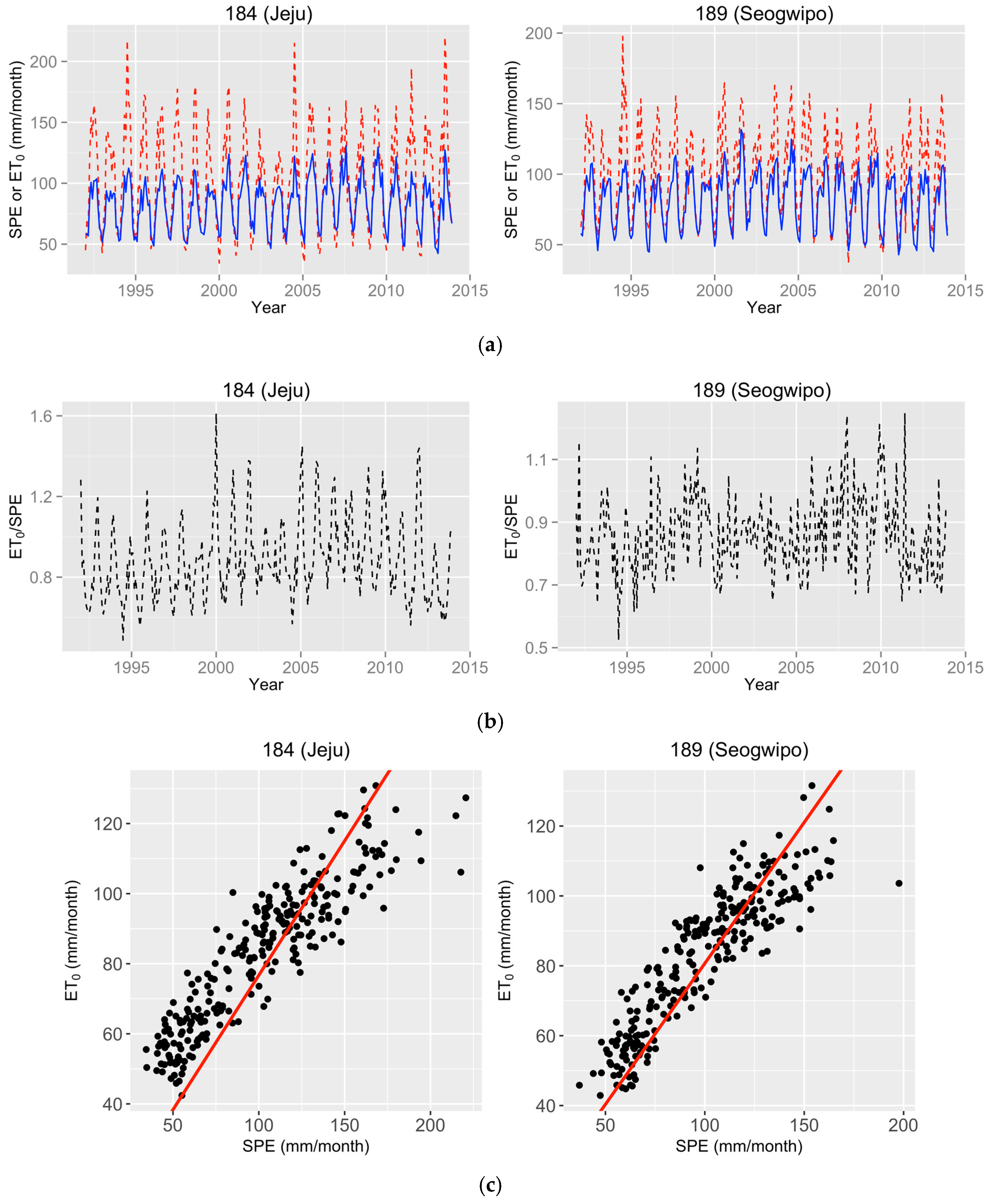
Using the extended meteorological data time series (e.g., EXT), we estimate the monthly reference crop ET at twelve sites where all four data types are available and compare the results to the monthly small pan evaporation data from January 1992 to December 2013 at the Jeju and Seogwipo stations (ID numbers 184 and 189, respectively) (Figure 3). These are the only two sites where small pan evaporation observations are available. The results (Figure 3a) show that the estimated reference crop ET values are significantly lower than the observed values during the summer, when ET rates peak over the course of a year. This seasonality is because pan evaporation tends to be overestimated during the summer when sunlight heats the sides and bottom of the metal pan and adds more energy to the water.
Figure 3b shows that the pan coefficient ranges from 0.49 to 1.61, with an average value of 0.88, at Jeju station and from 0.52 to 1.25, with an average value of 0.86, at Seogwipo station. These estimates are within a reasonable range in comparison to Allen et al. [7], who suggest that the coefficient ranges from 0.35 to 1.10. It is noted that the pan coefficients between two stations are not necessarily identical since Jeju and Seogwipo stations show different climate characteristics. Jeju is located in the northern end of the island with the mean annual precipitation of 1497.6 mm and Seogwipo is located in the southern end with the mean annual precipitation of 1923.0 mm. In this study, we focus evaluating the estimated reference crop ET indirectly with comparing to the SPE, the adjusted coefficients of determination (R2) between the two datasets are examined (Figure 3c). The R2 values at Jeju and Seogwipo are 0.97 and 0.98, respectively. According to these site-based results, we conclude that the estimated reference crop ET values based on the four meteorological parameters are reasonable; thus, spatial distribution maps are constructed in the following sections.
3.2. Regional Estimation
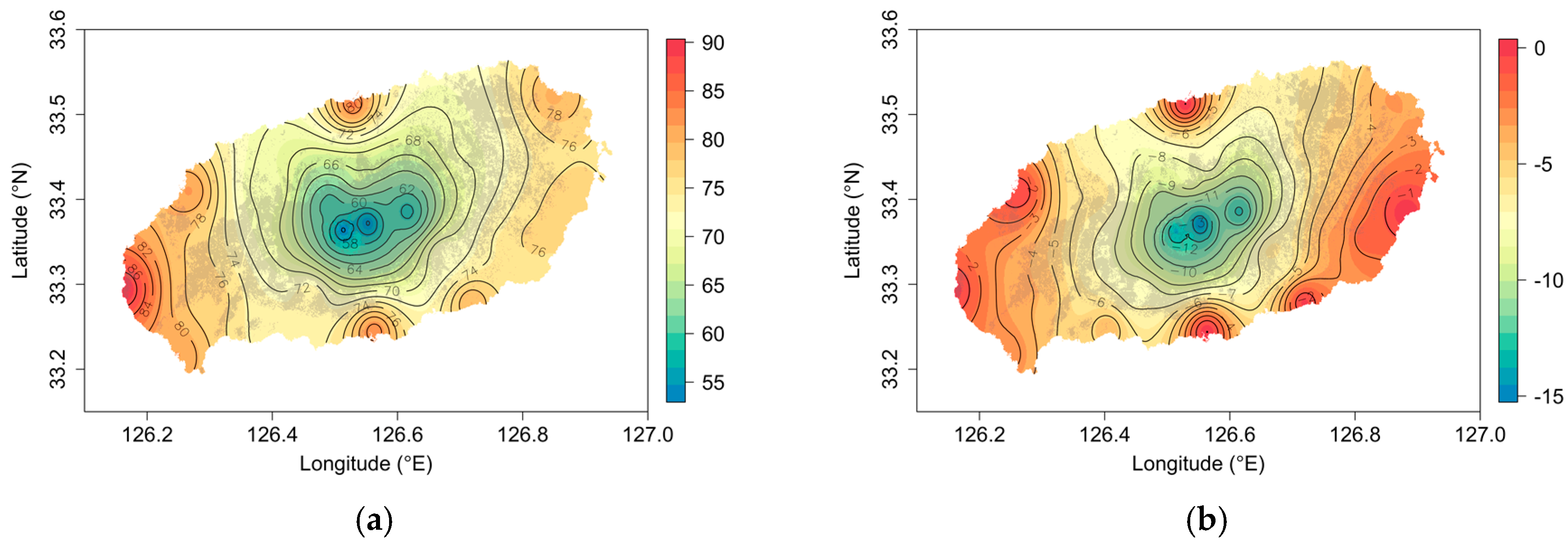
The regional monthly reference crop ET maps are constructed using the monthly climate maps. The regional maps of the four meteorological parameters are constructed based on both OBS and EXT data at the sites, and the reference crop ET maps are then constructed (Figure 4 and Figure 5). Because the available site data vary among the different sites, regional maps of each meteorological data type must be generated.
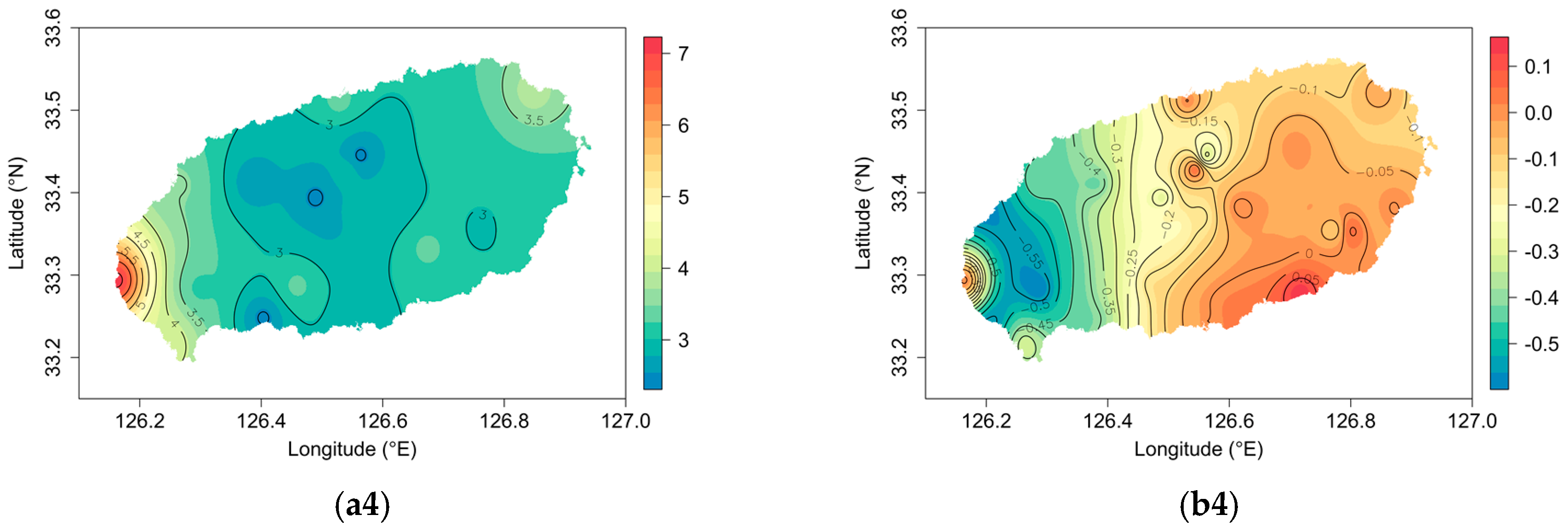
The meteorological data maps (Figure 4a) show the generally expected spatial patterns. With increasing elevation and distance from the coast, the temperature generally decreases, and the relative humidity and wind speed generally increases. The map of reference crop ET in Figure 5a shows that ET decreases with increasing elevation and distance from the coast. Thus, it closely follows the spatial patterns of air temperature and relative humidity. While the details will be investigated in the next section, one can expect a relatively limited effect of wind speed on ET in this region.
The different estimates based on EXT and OBS (Figure 4b and Figure 5b) show the effects of gap filling before spatial interpolation via hybrid Kriging in this study. Previous studies [16,17,18] show that the relatively large difference between EXT and OBS in the highlands corresponds to the fact that most of the observational stations are located in the lowlands, and maps based on OBS data cannot reasonably capture the spatial variability in the meteorological variables.
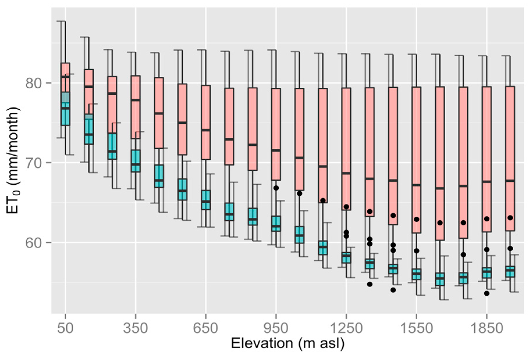
3.3. Spatial and Temporal Variations in Aggregated ETRC
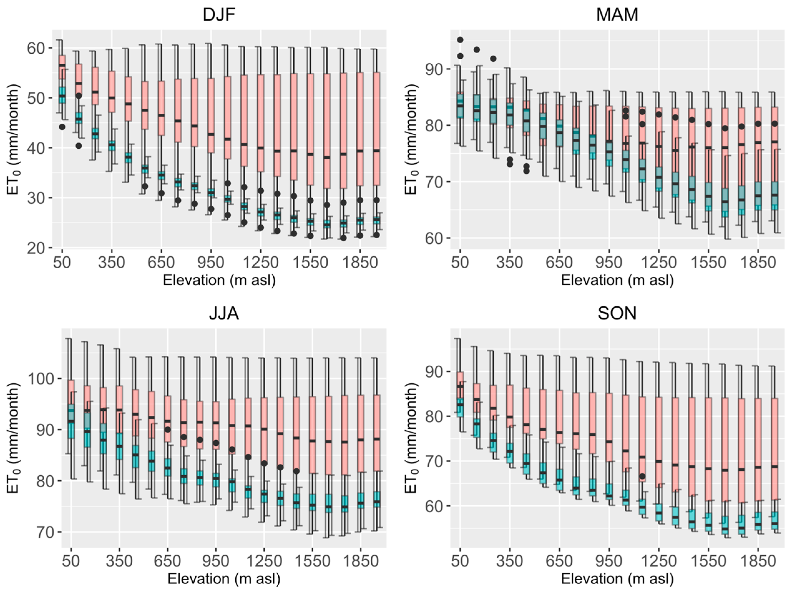
This study investigates the spatial and temporal variations in the aggregated reference crop ET values from Jeju Island. First, the aggregated reference crop ET according to elevation is investigated (Figure 6 and Figure 7). As expected, the values decrease gradually as the elevation increases. In a comparison between the EXT and OBS datasets, the range of estimated reference crop ET rates based on the OBS data is quite wide because the uncertainty increases in regions with high elevations due to limited data availability. Such elevation patterns for the annual average (Figure 6) are also shown in the seasonal averages and especially in fall and winter (Figure 7). The reference crop ET is estimated using EXT data with relatively small and similar uncertainties for different elevations and seasons.
Furthermore, focusing on the third quartile, the decreasing trend with elevation is not captured by the reference crop ET rates derived from the OBS data. These results indicate that the reference crop ET rates based on the EXT data better reflect the climate characteristics in regions with high elevations, suggesting that spatial interpolation using gap-filled site observations performs better than without the gap-filling process. Hereafter, only the results based on the EXT data are presented.
The decreasing trend is present only up to 1500 m a.s.l., and no trend is observed above this level. We therefore develop a linear model between the reference crop ET values and elevation for elevations below 1500 m a.s.l. in different seasons (Table 2). All of the linear models show an adjusted R2 value greater than 0.94. In winter (summer), the magnitude of reference crop ET is relatively small (large), and its rate of decrease with elevation is relatively large (small).
Investigating the 5-year moving averages of the reference crop ET, an overall increasing trend until the mid-2000s and a subsequent decreasing trend are found (Figure 8). These trends are maximized in Region 1 (R1) and minimized in Region 4 (R4). Westerly winds bring more moisture to R1, and orographic effects lead to more precipitation in the mountainous regions in R1. Therefore, ET is highest in R1 and could be significantly influenced by meteorological changes, such as temperature increases. The effects of different meteorological variables are investigated later in this section. Additionally, this study investigates the temporal trends in detail for different seasons in Figure 9. Most of the increasing trend until the mid-2000s present in the annual average is attributable to the increasing trends in spring (MAM in Figure 9) and summer (JJA in Figure 9). Few trends are observed in winter. Such temporal trends of reference crop ET mimic the temporal trends of average temperature as in Figure 10a of [16].
It is also noted that the studies have shown the decreasing trend of ET with attributing to different factors such as the decrease in solar radiation and wind speed. While Roderick et al. [23] suggested the role of decreasing solar radiation in decreasing pan evaporation, recent studies with observational data in China showed the different roles of solar radiation. Wang et al. [24] showed that the decrease in solar duration and wind speed were associated with the decrease in ET in China, but Shen et al. [25] suggested the impact of decrease in wind speed and temperature on decrease in ET in arid China.
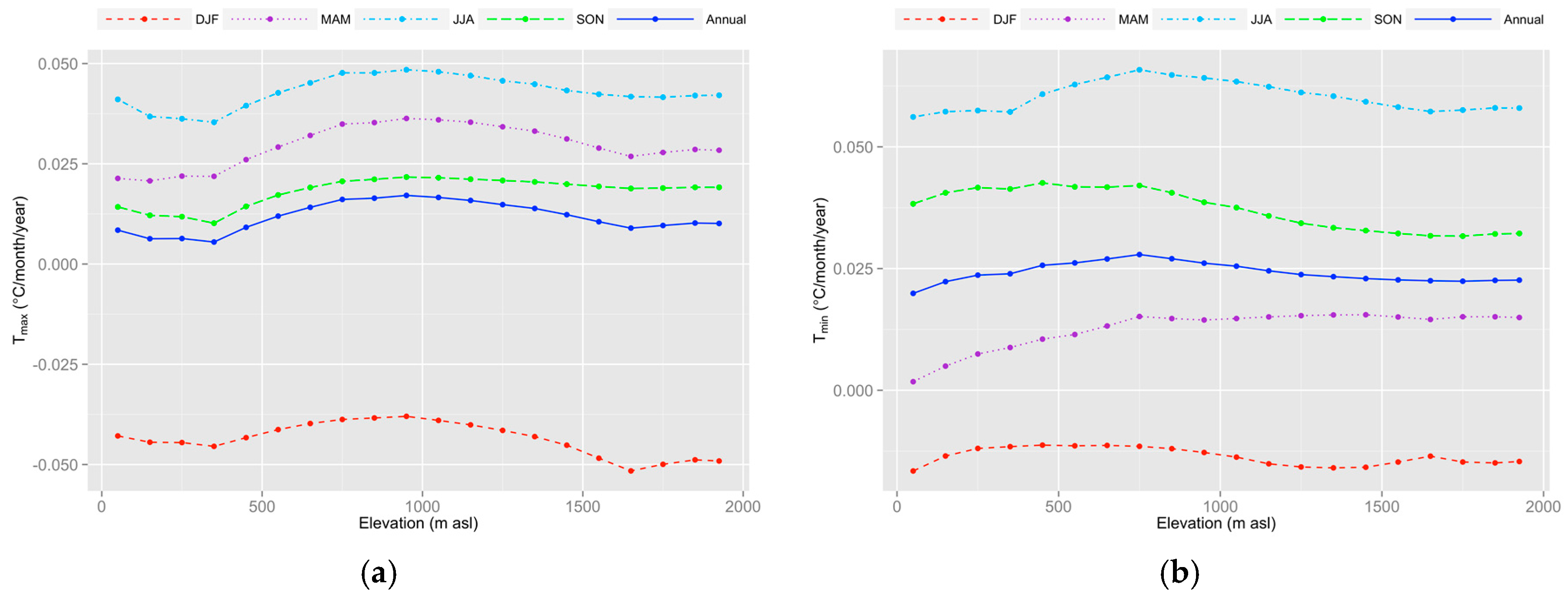
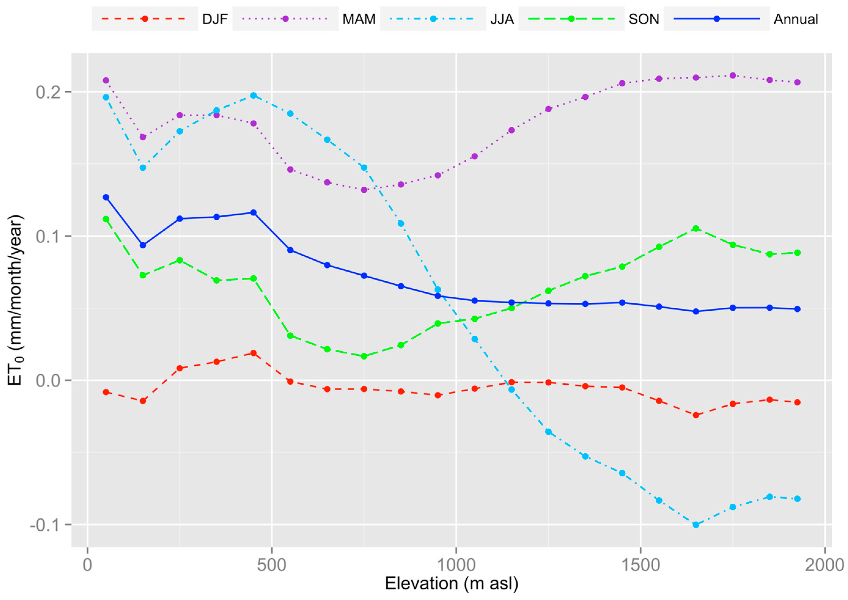
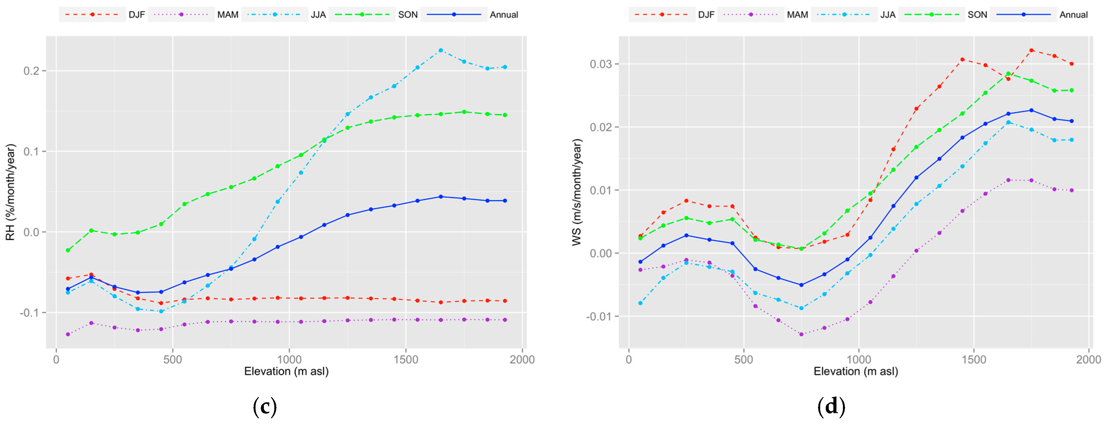
Figure 10 shows how the average temporal trends vary with elevation. In winter (DJF), there is no particular decreasing or increasing trends from low to high elevation, which is expected based on Figure 8. In summer (JJA), orographic changes are observed: the average temporal change in the reference crop ET is positive below 1000 m a.s.l. and negative above 1000 m a.s.l. To investigate these findings in detail, the four meteorological parameters used in this study are examined (Figure 11). The positive trends in relative humidity significantly increase with elevation in summer (JJA), resulting in a similar tendency in the reference crop ET in Figure 8. As in Equation (1), the reference crop ET is inversely proportional to RH.
Correlation analyses between the reference crop ET and other meteorological variables are performed for different seasons and different elevations (i.e., four elevation ranges: 0–500 m a.s.l., 500–1000 m a.s.l., 1000–1500 m a.s.l., and 1500–1950 m a.s.l.) (Table 3). In the region below 500 m a.s.l., the temporal trends in the reference crop ET values correlate significantly with temperature in all cases. These positive correlations are the most pronounced in spring regardless of the elevation. In winter, the relative humidity is associated with the ET most significantly because the evaporative demand controls ET during this time of year.
4. Conclusions
This study aims to understand the spatial and temporal variability in reference crop ET over Jeju Island, South Korea. Monthly reference crop ET maps are constructed using observed station-based meteorological data. Techniques including gap filling (i.e., PCR and MLR) and spatial analysis (i.e., hybrid Kriging) are then applied.
The results show various aspects of the variability in reference crop ET. With increasing elevation and distance from the coast, the air temperature decreases and RH increase; thus, the reference crop ET generally decreases. This study also observes increasing trends in the annual average reference crop ET values until the mid-2000s, with subsequent decreasing trends. This increase arises from the increasing trends in spring and summer. Very different temporal variations in ET at different elevations are also presented. For example, the summertime reference crop ET values show increasing temporal trends below 1000 m a.s.l. and decreasing temporal trends above 1000 m a.s.l. This difference is primarily due to the opposite temporal trends in RH. Note that such elevational variation is derived from the average reference crop ET for the whole study period from 1992 to 2013.
This study reveals previously unknown characteristics of reference crop ET that can be critical for agricultural and water resource management in this region. However, this study is limited to a relatively short time period with regard to the temporal variations due to limited data availability. The findings of this study, such as the different temporal trends in ET at different elevation levels, can be utilized for many different purposes, such as mountain management and development as well as agricultural land use planning.
Acknowledgments
This study was supported by the Korea Meteorological Administration R&D Program under the grant KMIPA 2015-6180 and by the Infrastructure and Transportation Technology Promotion Research Program funded by the Ministry of Land, Infrastructure and Transport of Korea (17RDRP-B076272-04). Yeonjoo Kim was also supported in part by the Yonsei University Future-leading Research Initiative of 2016 (2016-22-0061).
Author Contributions
Myoung-Jin Um and Yeonjoo Kim designed the study; Myoung-Jin Um performed the data analysis; Myoung-Jin Um, Yeonjoo Kim and Daeryong Park wrote the article.
Conflicts of Interest
The authors declare no conflict of interest.
References
- Zhang, Q.; Xu, C.Y.; Chen, Y.D.; Ren, L.L. Comparison of evapotranspiration variations between the Yellow River and Perarl River basin, China. Stoch. Environ. Res. Risk Assess. 2011, 25, 139–150. [Google Scholar] [CrossRef]
- Menzel, L.; Burger, G. Climate change scenarios and runoff response in the Mulde catchment (Southern Elbe, Germany). J. Hydrol. 2002, 267, 53–64. [Google Scholar] [CrossRef]
- Zuo, D.; Xu, Z.; Yang, H.; Liu, X. Spatiotemporal variations and abrupt changes of potential evapotranspiration and its sensitivity to key meteorological variables in the Wei River basin, China. Hydrol. Process. 2012, 26, 1149–1160. [Google Scholar] [CrossRef]
- Katul, G.G.; Parlange, M.B. A Penman-Brutsaert model for wet surface evaporation. Water Resour. Res. 1992, 28, 121–126. [Google Scholar] [CrossRef]
- Xu, C.Y.; Gong, L.B.; Jiang, T.; Chen, D.L.; Singh, V.P. Analysis of spatial distribution and temporal trend of reference evapotranspiration and pan evaporation in Changjiang (Yangtze River) catchment. J. Hydrol. 2006, 327, 81–93. [Google Scholar] [CrossRef]
- Digman, S.L. Physical Hydrology, 3rd ed.; Waveland Press: Long Grove, IL, USA, 2014; p. 643. [Google Scholar]
- Allen, R.G.; Pereira, L.S.; Raes, D.; Smith, M. Crop Evapotranspiration. Guide-Lines for Computing Crop Water Requirements; FAO Irrigation and Drainage Paper No. 56; FAO: Rome, Italy, 1998. [Google Scholar]
- Cristiano, P.M.; Campanello, P.I.; Bucci, S.J.; Rodriguez, S.A.; Lezcano, O.A.; Scholz, F.G.; Madanes, N.; Francescantonio, D.D.; Carrasco, L.O.; Zhang, Y.-J.; et al. Evapotranspiration of subtropical forests and tree plantations: A comparative analysis at different temporal and spatial scales. Agric. For. Meteorol. 2015, 203, 96–106. [Google Scholar] [CrossRef]
- McJannet, D.L.; Webster, I.T.; Cook, F.J. An area-dependent wind function for estimating open water evaporation using land-based meteorological data. Environ. Model. Softw. 2012, 31, 76–83. [Google Scholar] [CrossRef]
- McJannet, D.L.; Cook, F.J.; Burn, S. Comparison of techniques for estimating evaporation from an irrigation water storage. Water Resour. Res. 2013, 49, 1415–1428. [Google Scholar] [CrossRef]
- McMahon, T.A.; Peel, M.C.; Lowe, L.; Srikanthan, R.; McVicar, T.R. Estimating actual, potential, reference crop and pan evaporation using standard meteorological data: A pragmatic synthesis. Hydrol. Earth Syst. Sci. 2013, 17, 1331–1363. [Google Scholar] [CrossRef]
- McVicar, T.R.; van Niel, T.G.; Li, L.; Hutchinson, M.F.; Mu, X.; Liu, Z. Spatially distributing monthly reference evapotranspiration and pan evaporation considering topographic influences. J. Hydrol. 2007, 338, 196–220. [Google Scholar] [CrossRef]
- Li, Z.; Zheng, F.-L.; Liu, W.-Z. Spatiotemporal characteristics of reference evapotranspiration during 1961–2009 and its projected changes during 2011–2099 on the Loess Plateau of China. Agric. For. Meteorol. 2012, 154–155, 147–155. [Google Scholar] [CrossRef]
- Nam, W.-H.; Hong, E.-M.; Choi, J.-Y. Has climate change already affected the spatial distribution and temporal trends of reference evapotranspiration in South Korea? Agric. Water Manag. 2015, 150, 129–138. [Google Scholar] [CrossRef]
- Fry, M.M.; Rothman, G.; Young, D.F.; Thurman, N. Daily gridded weather for pesticide exposure modeling. Environ. Model. Softw. 2016, 82, 167–173. [Google Scholar] [CrossRef]
- Um, M.-J.; Kim, Y. Spatially variations in temperatures in a mountainous region of Jeju Island in Korea. Int. J. Climatol. 2016. [Google Scholar] [CrossRef]
- Um, M.-J.; Kim, Y. Spatial analysis of relative humidity during ungauged periods on mountainous Jeju Island, South Korea. Theor. Appl. Climatol. 2016. [Google Scholar] [CrossRef]
- Um, M.-J.; Kim, Y. Estimation of potential wind energy using data from sparsely located stations in a mountainous coastal region. Meteorol. Appl. 2017. [Google Scholar] [CrossRef]
- Cellura, M.; Cirrincione, G.; Marvuglia, A.; Miraoui, A. Wind speed spatial estimation for energy planning in Sicily: Introduction and statistical analysis. Renew. Energy 2008, 33, 1237–1250. [Google Scholar] [CrossRef]
- Teegavarapu, R.S.V. Floods in a Changing Climate; Cambridge University Press: Cambridge, UK, 2012. [Google Scholar]
- Hernandez-Escobedo, Q.; Saldana-Flores, R.; Rodriguez-Garcia, E.; Manzano Agugliaro, F. Wind energy resource in Northern Mexico. Renew. Sustain. Energy Rev. 2014, 32, 890–914. [Google Scholar] [CrossRef]
- Mojid, M.A.; Rannu, R.P.; Karim, N.N. Climate change impacts on reference crop evaportranspiration in North-West hydrological region of Bangladesh. Int. J. Climatol. 2015, 35, 4041–4046. [Google Scholar] [CrossRef]
- Roderick, M.L.; Farquhar, G.D. The cause of decreased pan evaporation over the past 50 years. Science 2002, 298, 1410–1411. [Google Scholar] [PubMed]
- Wang, Z.; Xie, P.; Lai, C.; Chen, X.; Wu, X.; Zheng, Z.; Li, J. Spatiotemporal variability of reference evapotranspiration and contributing climatic factors in China during 1961–2013. J. Hydrol. 2017, 544, 97–108. [Google Scholar] [CrossRef]
- Shen, Y.; Liu, C.; Liu, M.; Zeng, Y.; Tian, C. Change in pan evaporation over the past 50 years in the arid region of China. Hydrol. Process. 2010, 24, 225–231. [Google Scholar] [CrossRef]
Figure 1.
Study area and stations. (a) Elevation in m a.s.l.; (b) Land use; (c) Regions and stations; (d) Histogram of elevations of the stations. In (b), the eight types of land use are shown (1: Water, 2: Urban, 3: Bare ground, 4: Wetland, 5: Meadow, 6: Forest, 7: Paddy, 8: Field). In (c), R1 is region 1, R2 is region 2, R3 is region 3, R4 is region 4, and the number indicates the station number. The black dots are the weather stations for temperature and wind speed (WS), and the blue asterisks are the weather stations for relative humidity (RH).
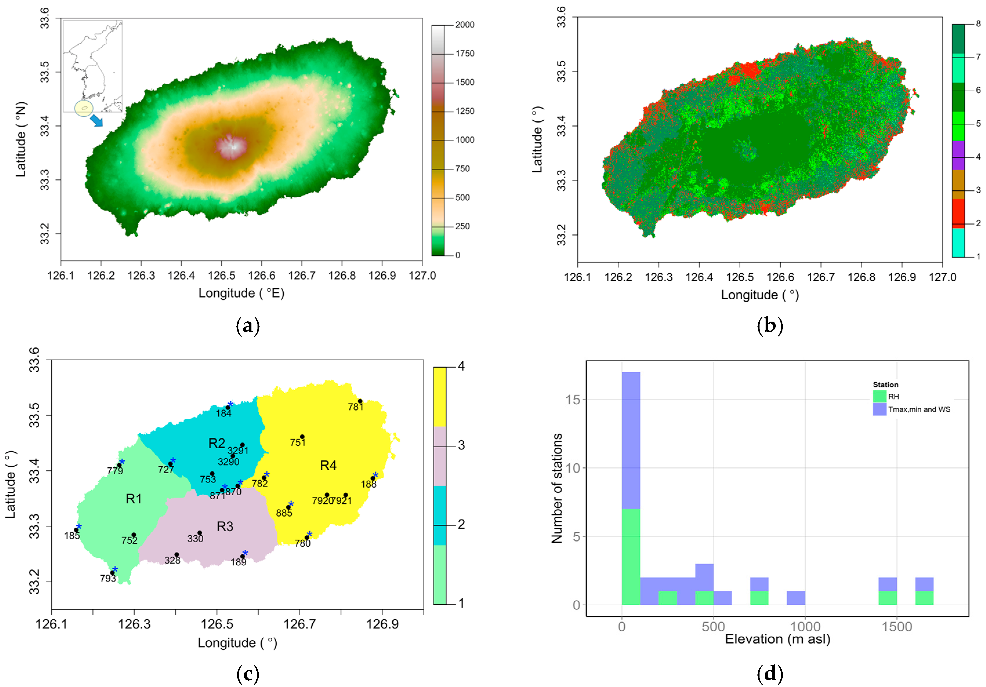
Figure 2.
Monthly box plots of climate data for all stations from 1992 to 2013. (a1) Observed monthly maximum temperature (Tmax) in °C; (a2) Extended monthly Tmax in °C; (b1) Observed monthly minimum temperature (Tmin) in °C; (b2) Extended monthly Tmin in °C; (c1) Observed monthly RH in %; (c2) Extended monthly RH in %; (d1) Observed monthly WS in m/s; (d2) Extended monthly WS in m/s.
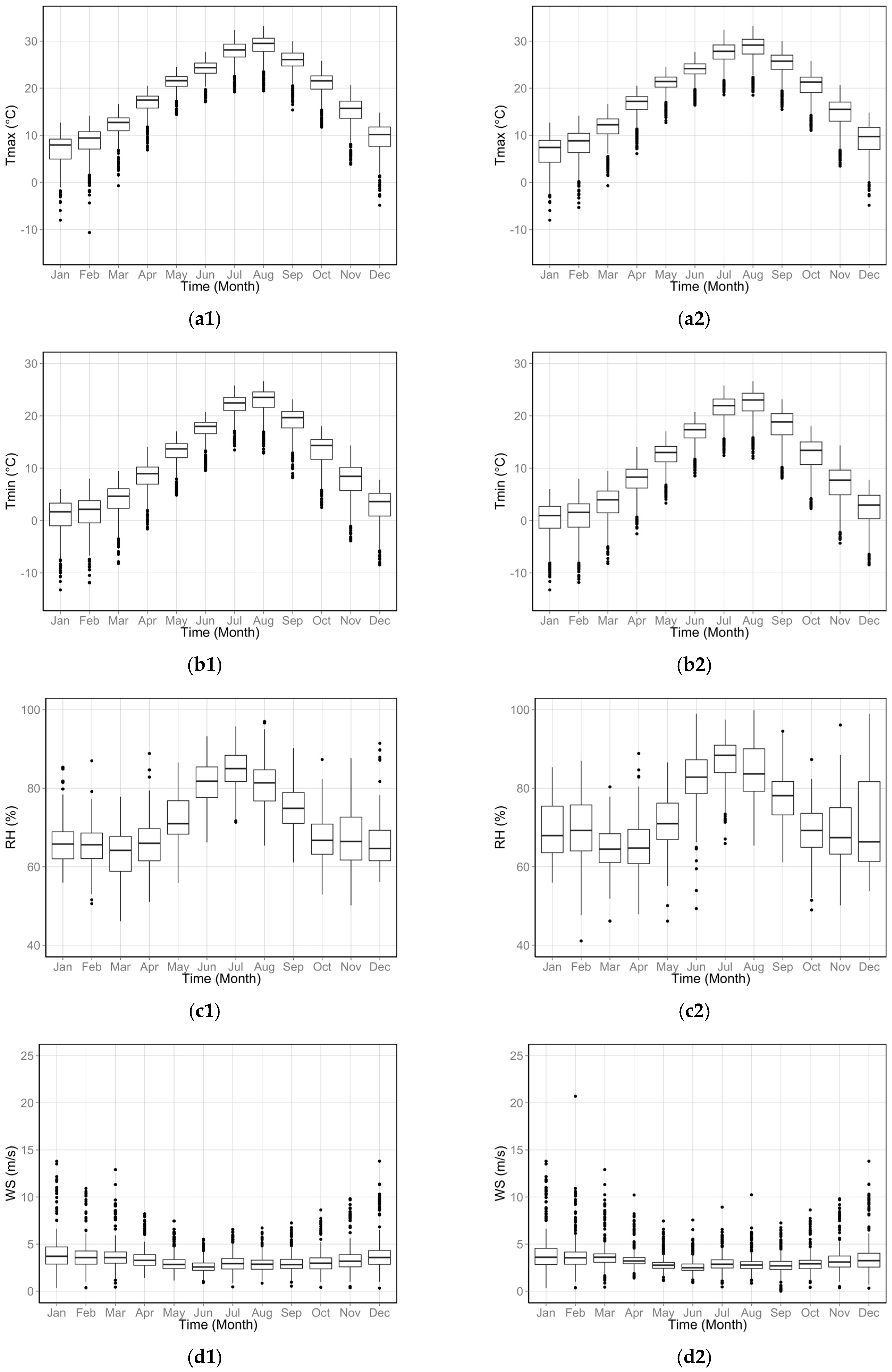
Figure 3.
Comparison between the reference crop evapotranspiration (ET) (ET0) and small pan evaporation (SPE) in mm/month at stations 184 and 189. (a) Monthly ET0 and SPE are indicated using blue and red dashed lines, respectively; (b) Monthly pan coefficient; (c) Scatter plot between monthly ET0 (y-axis) and SPE (x-axis) showing the linear regression line with an intercept of 0 based on Equation (4) (red line). The slopes of the lines at 184 and 185 are 0.76 and 0.81, respectively.

Figure 4.
Spatial distribution of (a) annual average monthly meteorological values of the extended data (EXT) and (b) the difference between extended and observed data (EXT-OBS). (a1) Tmax (EXT) in °C; (a2) Tmin (EXT) in °C; (a3) RH (EXT) in %; (a4) WS (EXT) in m/s; (b1) Tmax (EXT-OBS) in °C; (b2) Tmin (EXT-OBS) in °C; (b3) RH (EXT-OBS) in %; (b4) WS (EXT-OBS) in m/s.
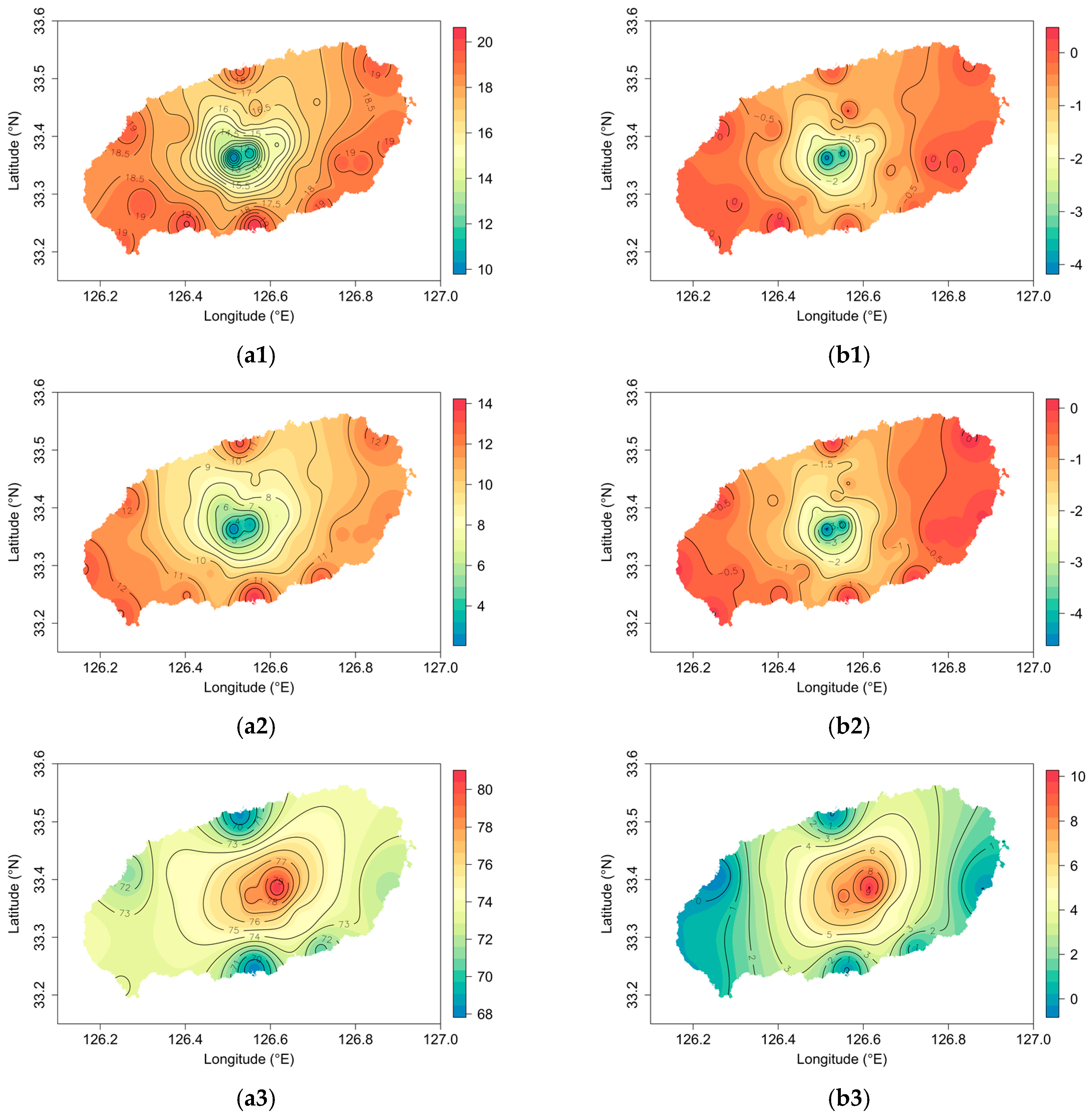

Figure 5.
Spatial distribution of (a) annual average monthly ET0 (mm/day) of EXT and (b) the difference between EXT and OBS (EXT-OBS). The shaded region represents the forest area (refer to Figure 1b).
Figure 5.
Spatial distribution of (a) annual average monthly ET0 (mm/day) of EXT and (b) the difference between EXT and OBS (EXT-OBS). The shaded region represents the forest area (refer to Figure 1b).

Figure 6.
Elevational changes in annual average monthly reference crop ET (ET0) in mm/month. Red and blue box plots represent OBS and EXT, respectively.
Figure 6.
Elevational changes in annual average monthly reference crop ET (ET0) in mm/month. Red and blue box plots represent OBS and EXT, respectively.

Figure 7.
Elevational changes in average monthly ET0 in mm/month for each season: DJF (December, January, and February), MAM (March, April, and May), JJA (June, July, and August), and SON (September, October, and November). Red and blue box plots represent OBS and EXT, respectively.
Figure 7.
Elevational changes in average monthly ET0 in mm/month for each season: DJF (December, January, and February), MAM (March, April, and May), JJA (June, July, and August), and SON (September, October, and November). Red and blue box plots represent OBS and EXT, respectively.

Figure 8.
Annual trend in the 5-year moving average of monthly ET0 in mm/month based on the extended climate data. The average for the whole study region is depicted as Total (solid blue line); the averages for R1, R2, R3, and R4 are presented using dashed red, dotted purple, dashed-dotted light blue, and dashed green lines, respectively.
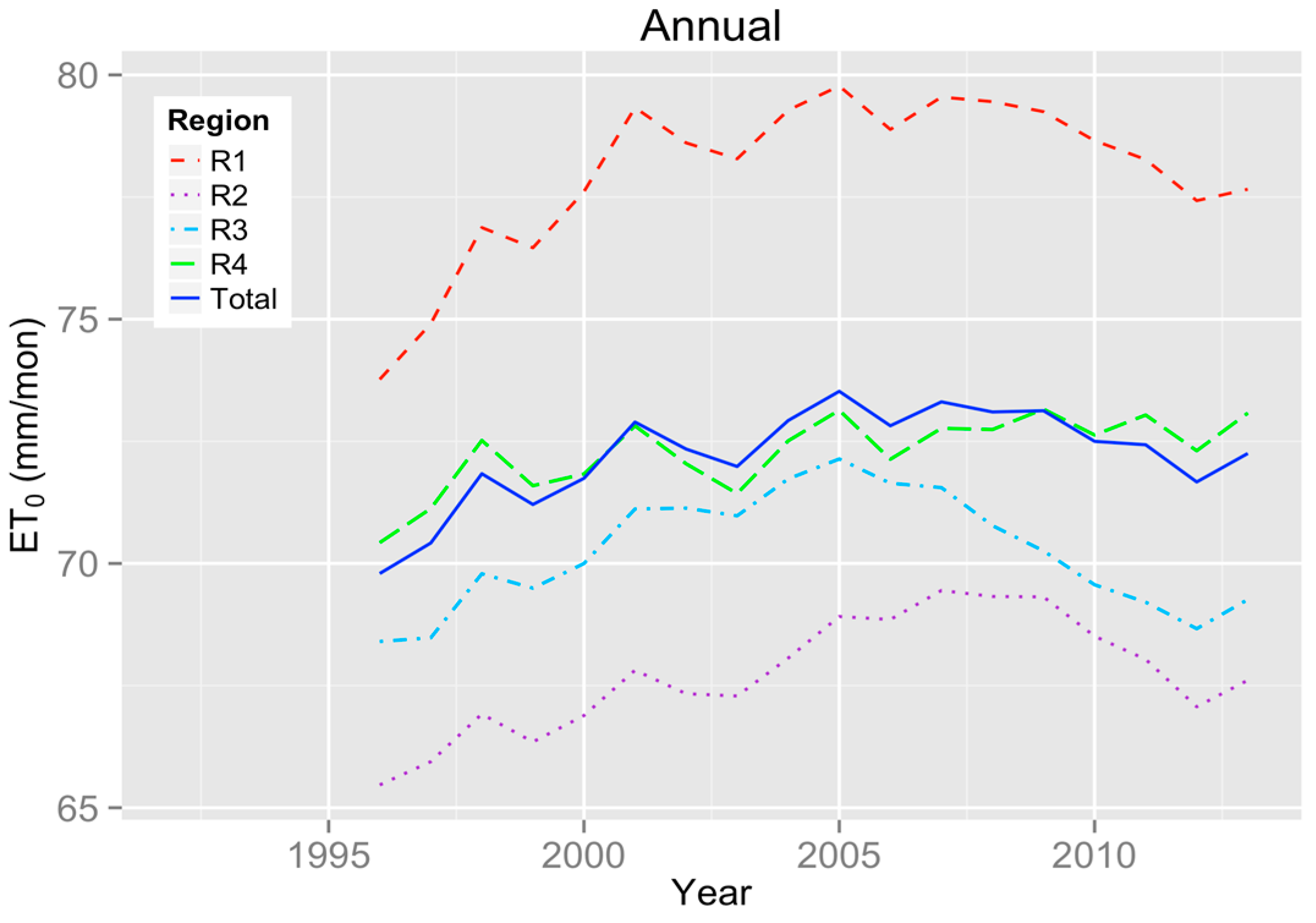
Figure 9.
Annual trend in the 5-year moving average of monthly ET0 in mm/month based on extended climate data for each season: DJF, MAM, JJA, and SON. The average for the whole study region is depicted as Total (solid blue line); the averages for R1, R2, R3, and R4 are presented using dashed red, dotted purple, dashed-dotted light blue, and dashed green lines, respectively.
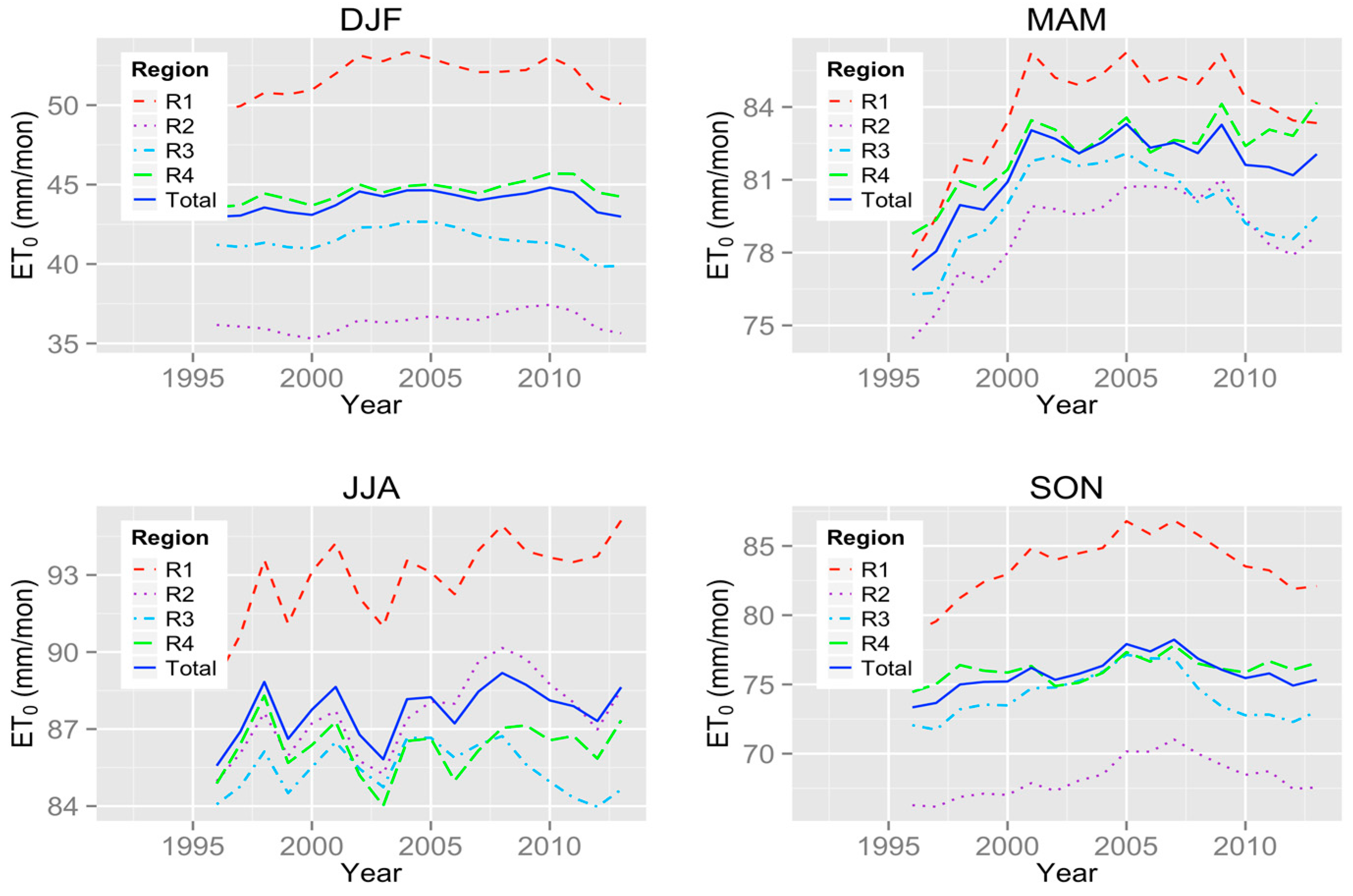
Figure 10.
Elevational variation in the annual change in monthly ET0. The solid blue line represents the annual average; the seasonal averages for DJF, MAM, JJA, and SON are presented using dashed red, dotted purple, dashed-dotted light blue, and dashed green lines, respectively.
Figure 10.
Elevational variation in the annual change in monthly ET0. The solid blue line represents the annual average; the seasonal averages for DJF, MAM, JJA, and SON are presented using dashed red, dotted purple, dashed-dotted light blue, and dashed green lines, respectively.

Figure 11.
Elevational variation in the annual change in monthly meteorological data. (a) Tmax; (b) Tmin; (c) RH; (d) WS. The solid blue line represents the annual average; the seasonal averages for DJF, MAM, JJA, and SON are presented using dashed red, dotted purple, dashed-dotted light blue, and dashed green lines, respectively.


Table 1.
Summary of models for temperature, relative humidity, and wind data.
| Variables | Models for Gap Filling | References |
|---|---|---|
| Daily Temperature (max., min.) | Principal component regression: Step (1) Principle component analysis (PCA): Daily temperature at multiple observed sites Step (2) Multiple linear regression : Daily temperature; : Independent variables from PCA; : Coefficients of the regression model. | [16] |
| Monthly Relative Humidity | Multiple linear regression: Monthly relative humidity; Location (in meters) corresponding to longitude in the transverse Mercator projection; Location (in meters) corresponding to latitude in the transverse Mercator projection; : Monthly temperature data; : Coefficients of the regression model. | [17] |
| Monthly Wind | Multiple linear regression: : Monthly wind speed; : Elevation; : Difference between the maximum and minimum temperatures; : Coefficients of the regression model. | [18] |
Table 2.
Relationships between ET0 based on extended data and elevations below 1500 m a.s.l.
| Season | Intercept | Slope | Adjusted R2 |
|---|---|---|---|
| DJF | 46.85 | −1.61 × 10⁻² | 0.94 |
| MAM | 84.59 | −1.06 × 10⁻² | 0.99 |
| JJA | 89.99 | −1.03 × 10⁻² | 0.97 |
| SON | 78.78 | −1.63 × 10⁻² | 0.94 |
| Annual | 75.05 | −1.33 × 10⁻² | 0.97 |
Table 3.
Correlation coefficients between ET0 and other meteorological variables (Tmax, Tmin, WS, and RH) for different seasons and elevation ranges.
Table 3.
Correlation coefficients between ET0 and other meteorological variables (Tmax, Tmin, WS, and RH) for different seasons and elevation ranges.
| Season | Elevation (m a.s.l.) | Tmax | Tmin | WS | RH |
|---|---|---|---|---|---|
| DJF | 0–500 | 0.631 | 0.631 | −0.105 | −0.303 |
| 500–1000 | 0.083 | −0.116 | 0.451 | −0.697 | |
| 1000–1500 | −0.090 | −0.351 | 0.492 | −0.851 | |
| 1500–1950 | −0.055 | −0.346 | 0.460 | −0.857 | |
| Total | 0.570 | 0.529 | −0.003 | −0.244 | |
| MAM | 0–500 | 0.951 | 0.916 | −0.706 | 0.281 |
| 500–1000 | 0.960 | 0.940 | −0.558 | 0.050 | |
| 1000–1500 | 0.967 | 0.953 | −0.435 | 0.018 | |
| 1500–1950 | 0.969 | 0.959 | −0.330 | −0.077 | |
| Total | 0.957 | 0.927 | −0.694 | 0.264 | |
| JJA | 0–500 | 0.854 | 0.741 | 0.163 | −0.460 |
| 500–1000 | 0.630 | 0.448 | 0.008 | −0.268 | |
| 1000–1500 | −0.055 | −0.251 | −0.273 | −0.664 | |
| 1500–1950 | −0.389 | −0.557 | −0.377 | −0.869 | |
| Total | 0.834 | 0.710 | 0.130 | −0.354 | |
| SON | 0–500 | 0.905 | 0.882 | −0.479 | 0.381 |
| 500–1000 | 0.898 | 0.867 | −0.363 | 0.022 | |
| 1000–1500 | 0.871 | 0.830 | −0.228 | −0.344 | |
| 1500–1950 | 0.871 | 0.827 | −0.152 | −0.414 | |
| Total | 0.906 | 0.881 | −0.464 | 0.304 |
© 2017 by the authors. Licensee MDPI, Basel, Switzerland. This article is an open access article distributed under the terms and conditions of the Creative Commons Attribution (CC BY) license (http://creativecommons.org/licenses/by/4.0/).
Share and Cite
MDPI and ACS Style
Um, M.-J.; Kim, Y.; Park, D. Spatial and Temporal Variations in Reference Crop Evapotranspiration in a Mountainous Island, Jeju, in South Korea. Water 2017, 9, 261. https://doi.org/10.3390/w9040261
AMA Style
Um M-J, Kim Y, Park D. Spatial and Temporal Variations in Reference Crop Evapotranspiration in a Mountainous Island, Jeju, in South Korea. Water. 2017; 9(4):261. https://doi.org/10.3390/w9040261
Chicago/Turabian StyleUm, Myoung-Jin, Yeonjoo Kim, and Daeryong Park. 2017. "Spatial and Temporal Variations in Reference Crop Evapotranspiration in a Mountainous Island, Jeju, in South Korea" Water 9, no. 4: 261. https://doi.org/10.3390/w9040261
Note that from the first issue of 2016, this journal uses article numbers instead of page numbers. See further details here.