The Spatial and Temporal Contribution of Glacier Runoff to Watershed Discharge in the Yarkant River Basin, Northwest China

Abstract

In this paper, a glacial module based on an enhanced temperature-index approach was successfully introduced into the Soil and Water Assessment Tool (SWAT) model to simulate the glacier runoff and water balance of a glacierized watershed, the mountainous region of the Yarkant River Basin (YRB) in Karakoram. Calibration and validation of the SWAT model were based on comparisons between the simulated and observed discharge with a monthly temporal resolution from 1961 to 2011 for the Kaqun hydrological station. The results reaffirmed the viability of the approach for simulating glacier runoff, as evidenced by a Nash–Sutcliff Efficiency (NSE) of 0.82–0.86 as well as a percentage bias (PBIAS) of −4.5% to 2.4%, for the calibration and validation periods, respectively. Over the last 50 years, the total discharge and glacier runoff both exhibited increasing trends with 0.031 × 10⁹ m³·a⁻¹ and 0.011 × 10⁹ m³·a⁻¹. The annual glacier runoff contribution to the streamflow was between 42.3% and 64.5%, with an average of 51.6%, although the glaciers accounted for only 12.6% of the watershed drainage area in the mountainous YRB. The monthly contribution of the glacier runoff ranged from 11.0% in April to 62.1% in August, and the glacier runoff from June to September accounted for about 86.3% of the annual glacier runoff. Runoff from the mountainous regions above 5000 m a.s.l. accounted for 70.5% of the total discharge, with glacier runoff contributions being approximately 46.4%.

1. Introduction

Affected by climate change, over the last few decades most glaciers around the world have appeared to be retreating at an accelerated rate [1,2,3,4], with a profound effect on the global water cycle. This has led to a considerable change in the hydrological processes within the respective watersheds that are supplied with snowmelt and glacier runoffs [5,6,7,8]. Understanding the spatial and temporal variations of snowmelt and glacier runoff is important because snowmelt and runoff are usually the pivotal sources of water supply at a regional scale [9,10,11,12]. Glacier runoff contributions to the total watershed discharge are also an essential part of climate change risk assessment and sustainable water management in the glaciated watersheds [13,14]. However, it is a challenging task to quantify the exact contribution of glacier runoff because of the complex interactions of the hydrological processes and the huge diversity of sources contributing to the stream runoff, as well as the mountainous topography and sophisticated accumulation and ablation processes on the glaciers in the glaciated alpine basins [15]. In terms of their contributions, the spatial and temporal variations of glacier runoff to the total discharge rate are highly uncertain for regional glacier systems [16,17,18].

In recent years, several studies have evaluated the contribution of glaciers to the hydrological cycle based on different methodological approaches including: direct discharge measurements [19,20], glaciological approaches [21,22], hydrological balance equations [10], hydrochemical tracers [23,24,25,26], and hydrological modeling [27,28]. Amongst them, hydrological modeling is the most frequently used approach for quantifying the contribution of the glacier runoffs [29]. Several models have been applied to study the contribution of runoff to the total watershed discharge [30], including but not limited to: Snowmelt Runoff Model (SRM) [4,26], Hydrologiska Fyrans Vattenbalans Model (HBV) [31,32], Glacier Evolution Runoff Model (GERM) [33,34], Flash-flood Event-based Spatially-distributed rainfall-runoff Transformation (FEST-WB) [28], J-2000 [35], Precipitation Runoff EVApotranspiration Hydrological response unit model (PREVAH) [15], Water flow and balance Simulation Model (WaSiM-ETH) [36], Variable Infiltration Capacity (VIC) [13], Topographic Kinematic Approximation and Integration Model (TOPKAPI) [11,37], Processes of Radiation, Mass and Energy Transfer (PROMET) [27], and the Soil and Water Assessment Tool (SWAT) [38,39]. In these hydrological models, the glacier runoff module can be classified into two kinds: energy balance models and temperature-index models [40]. Energy balance models, e.g., VIC, describe the physical processes of ablation with a high degree of precision and high degree of temporal resolution, but they need more detailed field observations and generally have a higher computational cost.

In the temperature-index models (e.g., SRM, GERM, FEST-WB, J-2000, PREVAH and SWAT), the melting rate is calculated from empirical formulas, neglecting some physical processes in some extent. However, the classical approaches applied to simulate the snow and ice melt, like the application of the distributed temperature-index method [40,41] or enhanced temperature-index method [42], are also the most common approaches. This is mainly because of their robustness in data-scarce regions [43], overall performance accuracy, and computational simplicity on a catchment scale. The SWAT model has been used for glacio-hydrological studies, for example by Luo et al. [38] and Rahman et al. [39,44]. However, the glacier melt algorithm in those studies was based on a classical degree-day model in the study of Luo et al. [38] which could not account for the spatial heterogeneities caused by local topography. Moreover, in the study of Rahman et al. [44] the glacier surface area was presumably static for a long time series, while the glacier surface area in the present study was dynamic, and thus provided a more robust simulation method.

Estimation of the long-term temporal and spatial variation of the glacier runoff contribution to total discharge for large basins offers signficant challenges because several hydrological models utilise coarse spatial resolution to simulate the water mass balance, whilst modeling the glaciers no doubt requires high resolution and detailed input data. The lack of observed data of high spatial resolution is also a significant obstacle [9]. Considering these pertinent issues, the objective of this study was to develop an approach for estimating the long-term temporal and spatial variation of glacier runoff contribution to total watershed discharge in the mountainous region of the Yarkant River Basin (YRB) in Karakoram, a large catchment with an area of 46,670 km². In this paper, the glacier module was based on enhanced temperature-index methods while the SWAT model was applied to simulate the glacier runoff and water balance. According to Radić and Hock [45], there are several concepts about ‘glacier runoff’ in literature. The glacier runoff mentioned in our study included all of the estimated runoff from the glacierized areas which encompassed snow and glacier melt runoff, rainfall runoff as well as all the other secondary runoffs. This outcomes of this study therefore, can serve as a useful guideline for assessing the climate change risks and sustainable water management issues in glaciated watersheds not only in the present region, but also in other regions worldwide where the glacial phenomenon exists.

2. Materials and Methods

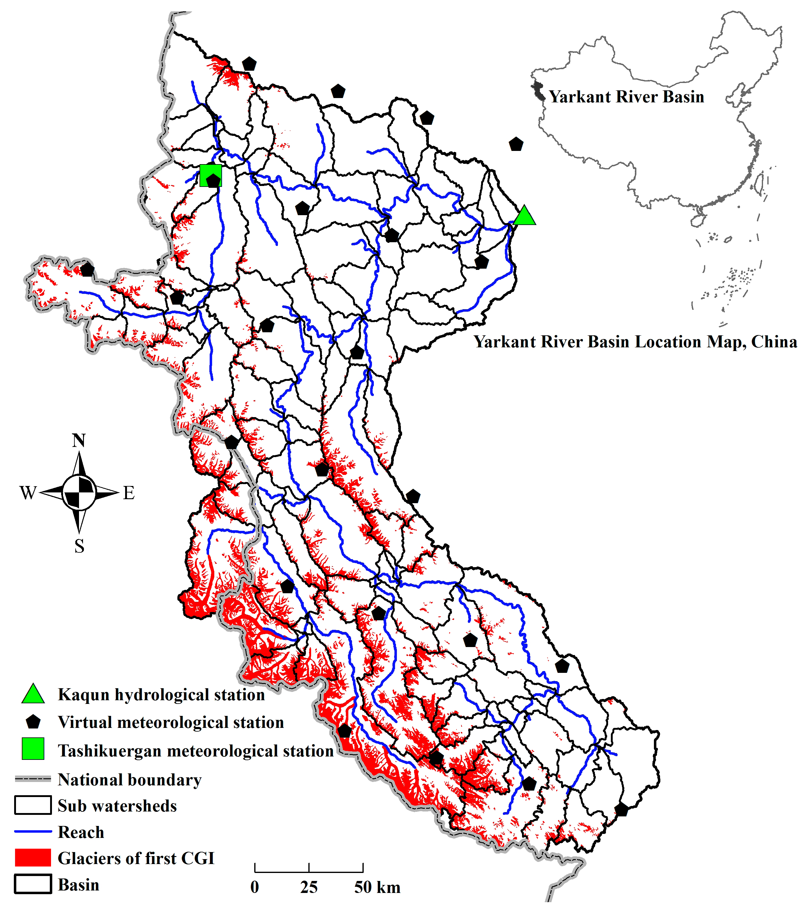
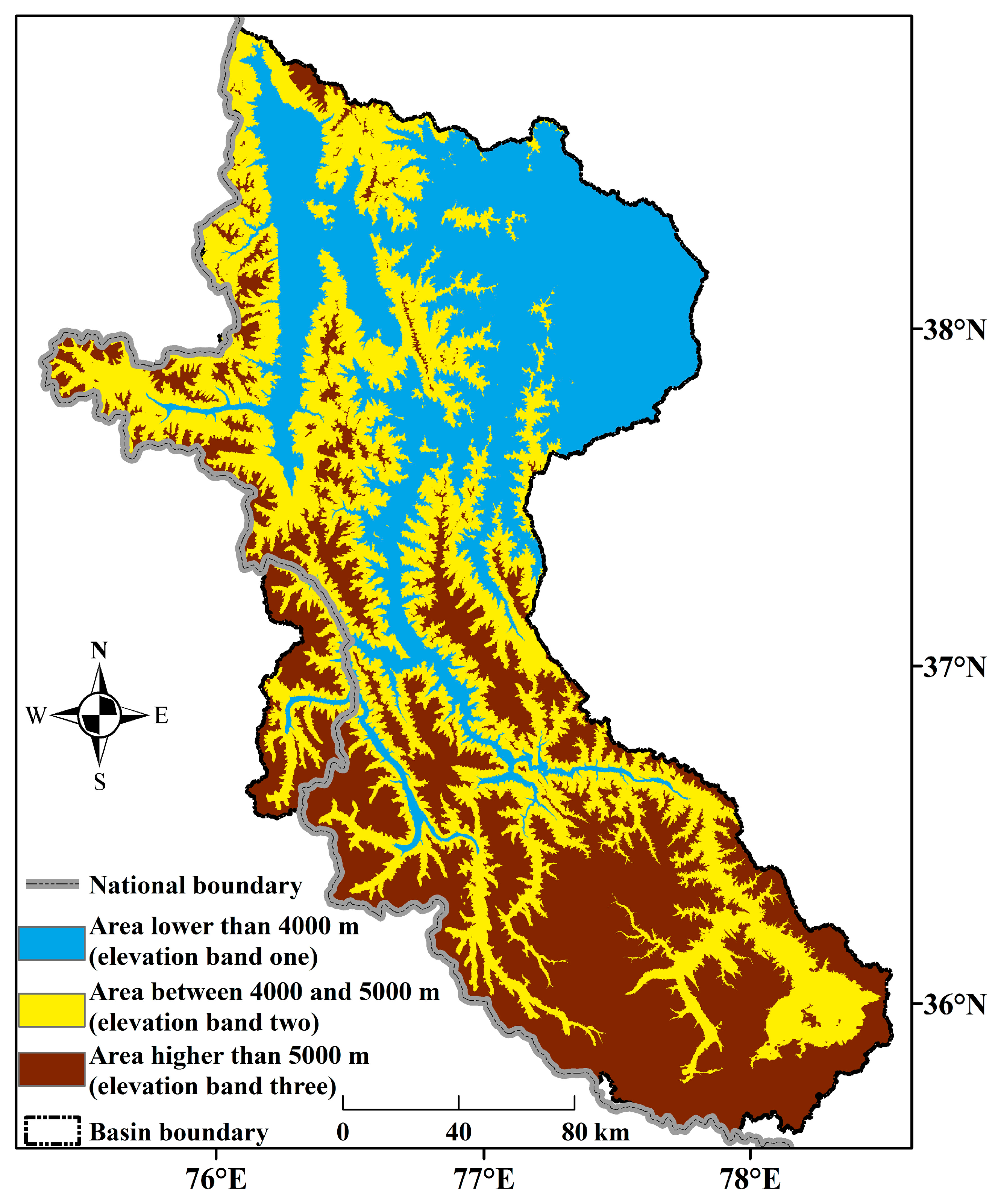
2.1. Study Area

Yarkant River Basin is situated in the western Tarim River Basin, on the northern slope of Karakoram [46,47]. The geographical range of the present study region extends from 35°24′ to 38°18′ N and 74°28′ to 80°54′ E, as shown in Figure 1. Elevation of YRB decreases gradually from south to north ranging from 1317 to 8569 m a.s.l. Many high mountains are located in the upper reaches of the YRB, which forms one of the world’s most developed mountain glacier regions. Valley glaciers are the main category of glaciers of the YRB [48]. Glaciers are distributed from 4000 to 8500 m a.s.l. There are as many as ten glaciers which are longer than 20 km and the areas covered by these glaciers are larger than 70 km², amongst which the Yengisogat Glacier (area is about 359 km²), is considered as the largest known glacier in China [46]. According to the first China Glacier Inventory (CGI), there are 3070 glaciers in the study regions with a total area of 5894.86 km² and a total volume of 690.25 × 10⁹ m³ [49].

The glacier runoffs of the YRB has been the primary supply for the Yarkant River [50]. According to the observation data of Kaqun hydrological station, the maximum and the minimum annual discharge of the YRB has been about 9.553 × 10⁹ m³ and 4.468 × 10⁹ m³, respectively, over recent decades. The total discharge is extremely unevenly distributed during a typical year, with about 74% of the annual discharge occurring from June to August and 26% in the other nine months [51]. The equilibrium line altitude for the region has an annual temperature of about −10.5 °C. The precipitation of YRB is greatly affected by the mountainous terrains, which results in an annual precipitation of 500 to 700 mm, 300 mm, and 150 mm, respectively, for high, middle, and low mountain belts [52].

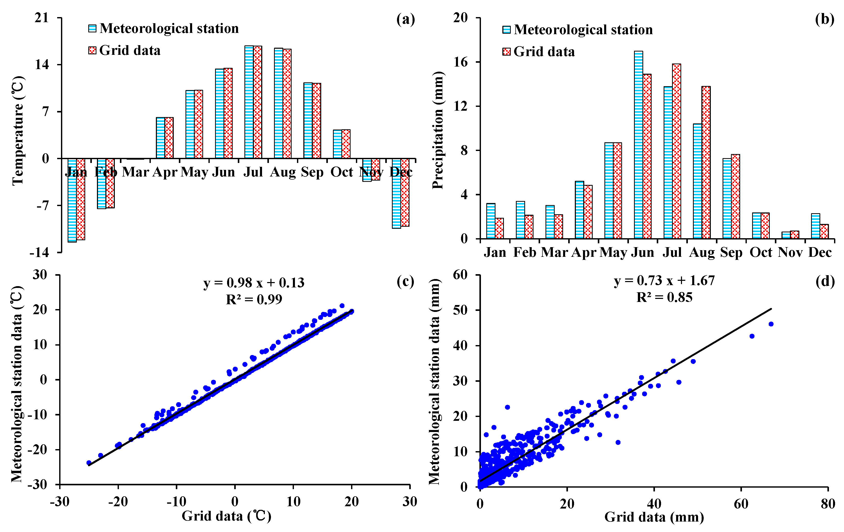
2.2. Meteorological and Hydrological Data

In YRB, there was a single meteorological site (known as the Tashikuergan station) from which the observed meteorological data, including daily maximum and minimum temperatures, precipitation, relative humidity, wind speed, and sunshine durations required for solar radiation calculations, were made available. Considering the sophisticated terrain and spatial extent of the present study area, the application of observation data from only one meteorological site can result in a high degree of uncertainty for any hydrological model. Therefore, the daily gridded precipitation and temperature data with a spatial resolution of 0.5 × 0.5 degrees were also acquired from the China Meteorological Administration (http://cdc.nmic.cn/). These datasets were developed by interpolating the 751 stations observations within China [53,54]. It is important to note that 0.5-degree gridded datasets are an official product checked through cross-validation and error analysis. Latest research [54] also showed that these 0.5 degrees gridded precipitation datasets can be considered as a good data product for representing the spatial characteristics of precipitation in significantly large terrains in northwest China.

In this research we compared the observation data recorded at Tashikuergan meteorological station with the data of the corresponding nearest grids using monthly air temperature and precipitation values. The results indicated that the coefficient of determination (R²) and the Nash–Sutcliff Efficiency (NSE) for mean, maximum and minimum temperatures were all greater than 0.90, and the R² and NSE values for precipitation were about 0.85 and 0.83, respectively. On the other hand, the bias of the mean monthly maximum temperature, minimum temperature, mean temperature and precipitation were about 0.11%, −6.75%, 1.85% and −1.27%, respectively, between Tashikuergan meteorological station and the nearest grid points. In Figure 2 we compare the meteorological station air temperature and precipitation data with the nearest grid point values.

In terms of meteorological station-based and gridded product, the temporal range of data in this paper was from 1 January 1961 to 31 December 2011. As such, there were 23 grids covered within the study area, which are generalized in Figure 1. Moreover, the daily relative humidity, wind speed, and solar radiation data were also acquired from the China Meteorological Forcing Dataset (available online: http://westdc.westgis.ac.cn/data/7a35329c-c53f-4267-aa07-e0037d913a21). It is noteworthy that this data has been proven to be the a suite of new, high-resolution dataset with a spatial resolution of 0.1 × 0.1 degrees [55]. In this study, the daily relative humidity, wind speed, and solar radiation data from the China Meteorological Forcing Dataset were upscaled to the 23 grids based on areal-mean method. Therefore, the 23 grid points could effectively be viewed as the virtual meteorological stations presenting daily maximum and minimum temperature, precipitation, relative humidity, wind speed, and solar radiation values.

Observed daily discharge data for the YRB were available at the watershed outlet of the Kaqun hydrological station. Among these data, the time series ranged from 1 January 1961 to 31 December 2008, with the missing data spanning from 1 January 1994 to 31 December 2000. Figure 1 shows the actual meteorological station, virtual meteorological station, and the corresponding hydrological station.

2.3. Underlying GIS-Referenced Data

SRTM 90-m digital elevation data were used as a digital elevation model (DEM) for the study area. GIS-referenced soil and land use data were downloaded from the portal of the Environmental and Ecological Science Data Center for West China (http://westdc.westgis.ac.cn), and extracted from a 1:1,000,000 soil map and a 1:1,000,000 vegetation map of China, respectively. There were 10 soil types and 11 land-use types in the study area. The soil and land use maps of the foreign portions (as shown in Figure 1) of the YRB were obtained from a Harmonized World Soil Database (HWSD) version 1.1 dataset and the Global Land Cover Database (GLC2000) dataset, respectively.

2.4. Glacier Data

Two periods for digital vector map of glaciers were obtained from the first and second China Glacier Inventory (CGI), based on aerial photos acquired during the period 1962–1977 for the first CGI, and remote sensing Landsat TM/ETM+ and ASTER images over the period 2004–2011 for the second. The first CGI data were used to determine the initial spatial distribution of the glaciers for the calibration period, while the second CGI data were similarly used for the validation period. There were 3070 glaciers in the study area with a total area of 5894.86 km² and a total volume of 690.25 × 10⁹ m³ for first CGI, and 3503 glaciers, with a total area of 5113.27 km², and total volume of 592.19 × 10⁹ m³ for the second CGI. The extent of glaciers for first CGI has been shown in Figure 1. In order to use accurate distribution map of the glaciers to drive the SWAT model, the CGI glacier map for the two periods were merged with the land use map for generating the hydrologic response unit in the SWAT model. Based on the underlying GIS-reference data and the glacier data, the study watershed was divided into 114 sub-watersheds and 2379 hydrologic response units (HRUs) including 182 glacier HRUs for the calibration period and 2382 HRUs including 185 glacier HRUs for the validation period.

The ice temperature melt factor was a crucial characteristic for glacier. We have collected several observed data in or around the study area (in the Tarim River Basin), as shown in

Table 1. Ice temperature melt factors of different observed glaciers in the Tarim River Basin.

Watershed	Glacier	Ice Temperature Melt Factor (mm·d−1·°C−1)	Altitude (m)	Observation Period
Yarkant River	Batura	3.4	2780	June–August 1975
	Teram Kangri	5.9	4630	25 June–7 September 1987
		6.4	4650	6 June–7 September 1987
Tailan River	Qirbulake	2.6	4750	6 June–30 July 1960
	Yangbulake	4.3	4800	1–5 July 1987
	Qiongtailan	4.5	3675	17 June–13 July 1978
		7.3	4100	25 June–31 July 1978
		8.6	4200	21 June–31 July 1978
Aksu River	Keqicar Baxi	4.5	3347	28 June–12 September 2003
		7.0	4216	11 July–13 September 2003

.

2.5. Description of SWAT

SWAT is essentially a watershed-scale, which is a physically based, continuous-time distributed simulation model [56]. The primary model components include: weather, water balance, energy balance, and soil temperature and its respective properties plant growth and land management [57]. In SWAT, a watershed is divided into multiple sub-watersheds, which are then further subdivided into hydrologic response units that consist of homogeneous land use, soil type, and the slope. The overall hydrologic balance is simulated for each HRU, including: the canopy interception of precipitation, partitioning of precipitation, snowmelt water, redistribution of water within the soil profile, evapotranspiration (ET), lateral subsurface flow from the soil profile, and the return flow from shallow aquifers. SWAT has been widely applied in a range of climatic, topographic, soil, and management conditions around the world to investigate a broad range of hydrological and environmental topics [58], including the cases of snow hydrology studies [59,60,61] and the glacial hydrology studies [38,39,44].

Elevation is considered as one of the most important variables in SWAT and it is intrinsically related to the meteorological parameters [62], especially in high alpine mountainous areas with sophisticated topography. Generally, SWAT allows the sub-watershed to be split into a maximum of ten elevation bands, and the temperature and precipitation for each band to be adjusted using t_laps and p_laps, respectively. A detailed description has been reported in the model documentation [61]. SWAT2005 is used in this study.

After preparation of forcing data, four major steps must be performed to set up the model: (1) watershed discretization and sub-watershed characteristics derivation; (2) definition of the HRU; (3) running of the model and analysis of the parameter sensitivity; and (4) calibration and validation of the SWAT model, including uncertainty analysis.

2.6. Glacier and Snow Melt Algorithm

2.6.1. Snow Melt Algorithm

SWAT distinguishes precipitation as being either rain or snow in terms of the mean daily temperature. The threshold temperature used to categorize precipitation either as rain or snow is defined by the user. If the mean daily air temperature is lower than the threshold temperature, then the precipitation will be modeled as snow, and the water equivalent will be added to the snow pack. If the mean daily air temperature is higher than the threshold temperature, then the precipitation will be modeled in the form of liquid rain. The snow pack will thus increase with the additional snowfall or will decrease with the snowmelt or sublimation process, while the water stored in the snow pack will be reported as a snow water equivalent.

In this case study, the temperature index with an elevation band approach was applied to simulate the snowmelt [39,40]. Snowmelt in the SWAT can be calculated as a linear function of the difference between the average snow pack-maximum air temperature and the threshold temperature for snowmelt. A detailed description has been reported in the model documentation [57].

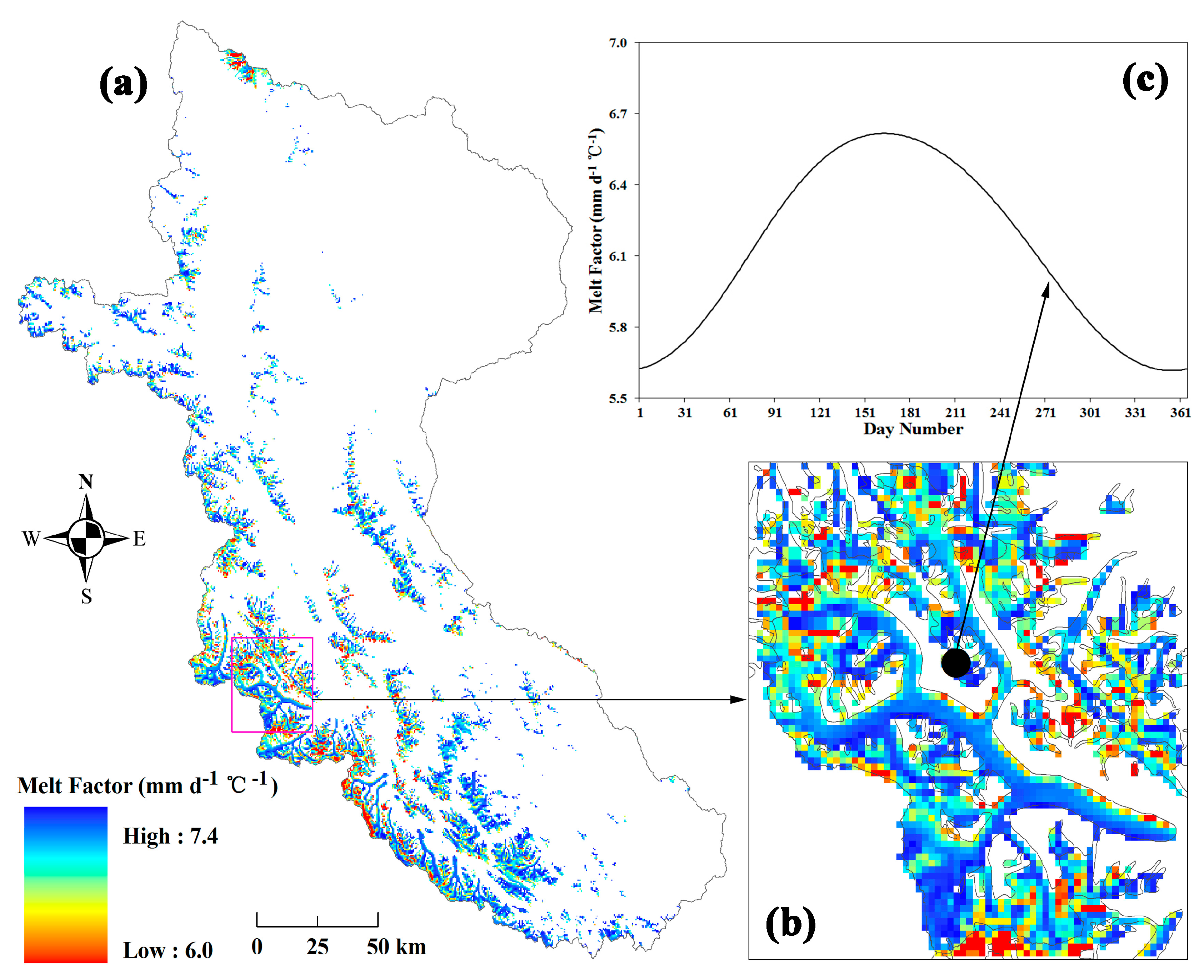
2.6.2. Glacier Melt Algorithm

An enhanced temperature-index approach was applied for glacier melt modeling. This is able to calculate the melting of glacial ice based on a linear relationship between ablation and positive air temperature, and includes the effect of potential solar radiation, thus accounting for the spatial heterogeneities induced by topography [40]. The local melt rate, M, is calculated in the daily resolution using:

$$M=\{\begin{array}{lll}(F_M+r_{ice}{I}_{pot})\cdot (T-T_{mlt,ice})\hfill & :& T>T_{mlt,ice}\\ 0\hfill & :& T\le T_{mlt,ice}\end{array}$$

(1)

where F_M is the ice temperature melt factor, r_ice is the ice radiation melt factor, F_M + r_iceI_pot is called the ice melt factor hereinafter and I_pot denotes the potential solar direct radiation, with T as the mean daily air temperature whereby the temperature below T_mlt,ice can indicate that no melting has occured. Daily air temperature for each elevation band is computed using a constant temperature lapse rate, t_laps, and similarly, the precipitation lapse rate, p_laps, is also computed assuming a linear increase with increasing elevation. The potential direct solar radiation, I_pot, is calculated as a function of the top-of-atmosphere solar radiation, atmospheric transmissivity, solar geometry, and the topographic characteristics [63] using:

$$I_{pot}=S{\left(\frac{d_m}{d}\right)}^2{\psi }^{\frac{P}{P_0\cos Z}}\left[\cos \theta \cos Z+\sin \theta \sin Z\cos \left({\varphi }_{sun}-{\varphi }_{slope}\right)\right]$$

(2)

where S = 1360 W·m⁻² is the solar constant, (d_m/d)² is the eccentricity correction factor of the Earth’s orbit, ψ = 0.75 is the mean atmospheric clear-sky transmissivity, P is the atmospheric pressure, P₀ is the mean atmospheric pressure at sea level, Z is the zenith angle (approximated as a function of latitude, solar declination, and hour angle), θ is the slope angle, φ_sun is the solar azimuth angle, and φ_slope is the slope azimuth angle (aspect).

In the simulation algorithm, the potential direct solar radiation is set to zero between the sunset and sunrise period and for the surface that is shaded by the surrounding topography. By including the potential direct solar radiation I_pot in Equation (1), both the diurnal and spatial variations for calculating the melt are taken into account.

The refreezing can be calculated via defining a ratio of melt water, and the refreezing ratio has been set to 0.2, determined at an observed glacier, Qiyi Glacier, in the Qilian Mountains in Northwest China [64].

2.6.3. Glacier Area Changes

According to the measurements conducted over sixteen glaciers based on radar technology in northwest China by Liu et al. [65], the relationship between the glacial surface area and the volume can be represented by:

$$V_g=0.04\cdot {A_g}^{1.35}$$

(3)

where A_g is glacial surface area (km²) and V_g is the glacial volume (km³).

The data assembled by Meier and Bahr [66] suggested a similar relationship between the area and volume, with a mean exponent value of 1.36. The relationship between the glacier volume, glacier area and the depth of water equivalent of a glacial mass can be expressed as:

$$V_g=\frac{W_g\cdot A_g}{{\rho }_i}$$

(4)

where W_g is the equivalent water depth of ice and ρ_i is the bulk density of ice (usually, 900 kg·m⁻³).

Of note, the initial value of W_g can be calculated by the glacial surface area obtained from the CGI data. Next, the glacial water equivalent can be adjusted according to the respective day’s M value, so that the glacial area can be easily derived using Equations (3) and (4).

2.6.4. Glacier Accumulation Rate

Glaciers are almost always dynamic, and therefore, they are characterised by an accumulation and ablation process, with the accumulation occurring in the cold season and the ablation and accumulation both taking place during the warm season. To capture the seasonal and gradual patterns of the accumulation process and while maintaining the simplicity of the method, Luo et al. [38] proposed an algorithm to account for the accumulation of glacier mass by simulating the glacier process in the Tianshan Mountain of Western China. The turnover of the snow to an ice form is represented as a ratio of the water equivalent of the snow over ice and can be given as:

$$F=\beta \cdot W_s$$

(5)

where W_s is the water equivalent of snow over ice in mm, and β is an accumulation coefficient (assumed to be changing seasonally), given as below:

$$\beta ={\beta }_0\left\{1+\sin \left[\frac{2\pi }{365}(t-81)\right]\right\}$$

(6)

In Equation (6), β₀ is the basal accumulation coefficient. It is imperative to note that the accumulation rate changes seasonally to the high value on 21 June and the low value on 21 December, implying that a greater proportion of the snow water may change into ice in the summer compared to the winter period.

2.7. Model Performance Evaluation

Several studies have proposed a standard hydrological model performance criterion. For this study we followed NSE, Root Mean Square Error (RMSE)-observations standard deviation ratio (RSR), and percentage bias (PBIAS) as the model evaluation statistic [67]. Model performances were considered ‘very good’ which was the best level stipulated by 0.75 < NSE ≤ 1.0, and 0.0 ≤ RSR ≤ 0.50, and PBIAS < ±10, respectively. Note that the NSE is a normalized statistic that can determine the relative magnitude of the residual variance (“noise”) in the modelled data compared to the measured data variance (“information”). The NSE can also indicate how well the plots of observed versus simulated data fit the 1:1 line of agreement where Q_obs,i is the observed data value at time, i, and Q_sim,i is corresponding the simulated data value. NSE values lie between −∞ and +1 where +1 indicates an optimal model performance.

$$NSE=1-\frac{{\displaystyle \sum _{i=1}^n{\left(Q_{obs,i}-Q_{\mathrm{sim},i}\right)}^2}}{{\displaystyle \sum _{i=1}^n{\left(Q_{obs,i}-Q_{obs,avg}\right)}^2}}$$

(7)

$$RSR=\frac{RMSE}{STDE{V}_{obs}}=\frac{\sqrt{{\displaystyle \sum _{i=1}^n{\left(Q_{obs,i}-Q_{sim,i}\right)}^2}}}{\sqrt{{\displaystyle \sum _{i=1}^n{\left(Q_{obs,i}-Q_{obs,avg}\right)}^2}}}$$

(8)

$$PBIAS=\frac{{\displaystyle \sum _{i=1}^n\left(Q_{\mathrm{sim},i}-Q_{obs,i}\right)}}{{\displaystyle \sum _{i=1}^n{Q}_{obs,i}}}\times 100$$

(9)

The RMSE-observations standard deviation ratio (RSR) is calculated as the ratio of the RMSE (Root Mean Square Error) and the standard deviation of the observed (measured) data. Note that the RMSE is one of the most commonly used error index statistics, whereby a lower value indicates a better model performance. In fact, the RSR value standardizes the RMSE value using the observations standard deviation, and therefore, it incorporates the benefits of the error index statistics and standard deviation of the measured data. In terms of its magnitude, the RSR varies from an optimal value of 0, which indicates zero RMSE or zero residual variation and a perfect model simulation, to a large positive value that represents an inaccurate model simulation. A low RSR is expected to result from a low RMSE, and therefore, will indicate good model simulation performance.

Applied for error assessments, the PBIAS statistic (in %) can be used to assess the average tendency of the model simulated data to be larger or smaller than their corresponding observed values. PBIAS can be utilized as an indicator of the under- or over- estimation of the observed data; and in fact, negative PBIAS values can indicate an underestimation of the model results relative to the measured conditions.

3. Results and Discussion

3.1. Calibration

In this paper, there was only one meteorological station located within the study area, so the gridded temperature and precipitation datasets with a spatial resolution of 0.5 × 0.5 degrees were selected to force the simulation model. However, the region covered by each grid extended several tens of square kilometers. Uncertainty derived from input data were reduced by adjusting the temperature and precipitation via the setting up of t_laps and p_laps parameters as well as dividing the sub-watersheds into several elevation bands. Every sub-watershed was divided into ten elevation bands in this study. The t_laps (5.0 °C/km) and p_laps (155 mm/km) were calculated and then optimized from the statistical relationships of elevation with annual temperature, and annual precipitation data of the 23 virtual meteorological stations.

The ice melt factor (F_M + r_iceI_pot) in Equation (1) was set to vary continuously according to the temporal and spatial variations. We also calculated the spatial distribution of ice melt factor for the 182nd day in a year as an example, as shown in Figure 3a. It was obvious that the ice melt factor was different because of the different slopes, aspect, latitude, and so on. Figure 3b shows the partially enlarged drawing, to provide a clear view of the spatial heterogeneities of the ice melt factor. The temporal variation of ice melt factor for the dots represented in Figure 3b was also calculated and has been shown in Figure 3c to provide a demonstration of the temporal variation of the ice melt factor in a year.

The hydrological model was calibrated for the time series from 1 January 1961 to 31 December 1988, with the period from 1 January 1961 to 31 December 1964 as a ‘warm-up’ phase. Glacier coverage was based on the first CGI. We applied a ‘trial-and-error’ method to calibrate the model including the glacial module parameters F_M, r_ice, and β₀. The parameter set of the previous related studies in or around the study area were also referenced. It is also important to mention that the ice temperature melt factor was a crucial parameter for the glacier module. According to the results of the ice temperature melt factors of different observed glaciers in the Tarim River Basin (Table 1) [68], we set the nominal value of F_M to be 5.5 mm d⁻¹·°C⁻¹. Following the study of Manas River Basin in the Tianshan Mountains in Northwest China [38], the value of β₀ was adoted to be 0.003 in our work. The radiation coefficient for ice was set to 14.4 × 10⁻⁶ m³·W⁻¹·d⁻¹·°C⁻¹, according to a study performed in the source region of Yangtze River in western China [69].

Table 2. Calibrated parameters and their optimized values.

Model Routine	Parameter	Description	Range	Optimized Value
Snow	SMFMX	Melt factor for snow, 21 June (mm/°C-day)	0, 10	6.5
	SMFMN	Melt factor for snow, 21 December (mm/°C-day)	0, 10	1.0
	SFTMP	Snowfall temperature (°C)	−5, +5	1.0
	SMTMP	Snow melt base temperature (°C)	−5, +5	0.5
	TIMP	Snow pack temperature lag factor	0.1, 2.0	1.0
Glacier	FM	Melt factor for ice (mm/°C-day)	2.6, 13	5.5
	rice	Radiation factor for ice	0, 0.1	14.4 × 10−6
	β0	Basal accumulation coefficient	0.001, 0.006	0.003
Runoff	ESCO	Soil evaporation compensation factor	0.01, 1.0	0.55
	ALPHA_BF	Baseflow alpha factor (days)	0.1, 1.0	0.036
	CN2	Initial SCS CN II value	50, 80	Multiply 70%
	CH_K2	Effective hydraulic conductivity in channel (mm/h)	0, 50	4
	GWQMN	Threshold depth of water in shallow aquifer (mm)	1, 200	100
	GW_DELAY	Groundwater delay (days)	0, 180	45

shows the calibrated parameters and their optimized values.

After determining the optimal calibrated values (mainly based on the stream discharge and observed glaciers) for all selected parameters, the calibrated values were then reused in the validation period from 1 January 1985 to 31 December 2011, with a warm-up period from 1 January 1985 to 31 December 1988. The glacier coverage during the validation period was based on the second CGI and the model performance was evaluated by calculating the set of objective functions (i.e., NSE, RSR, and PBIAS as per Equations (7)–(9)).

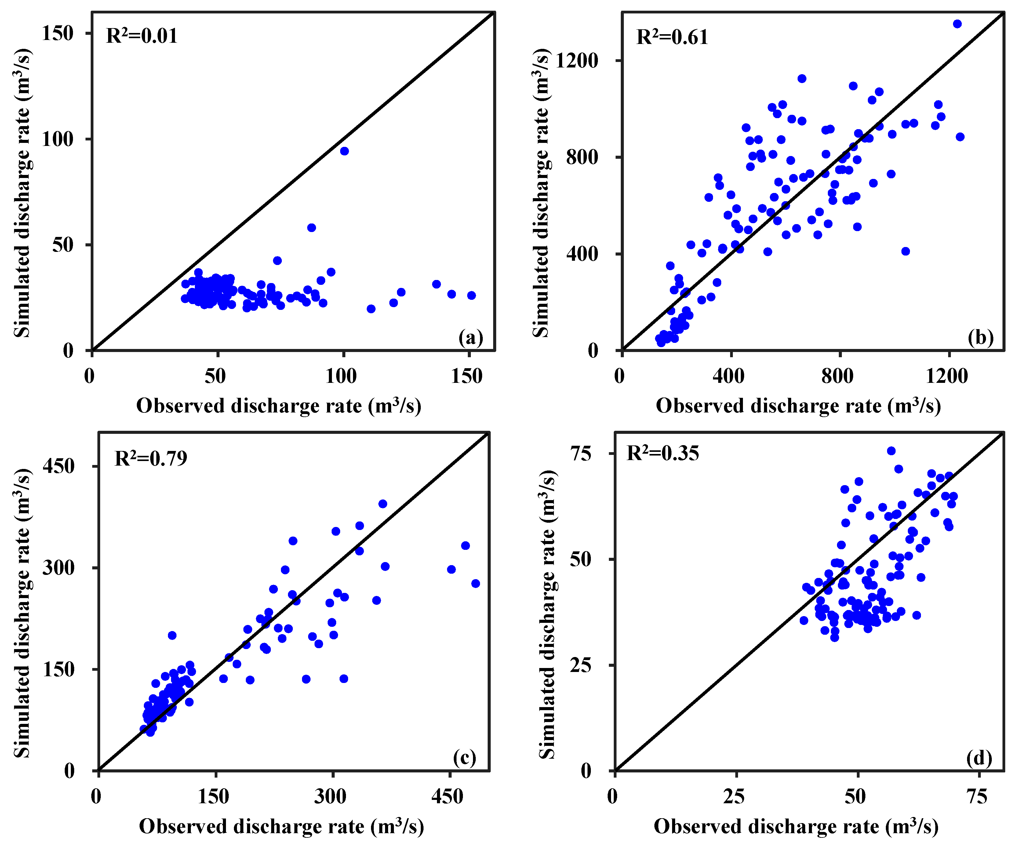
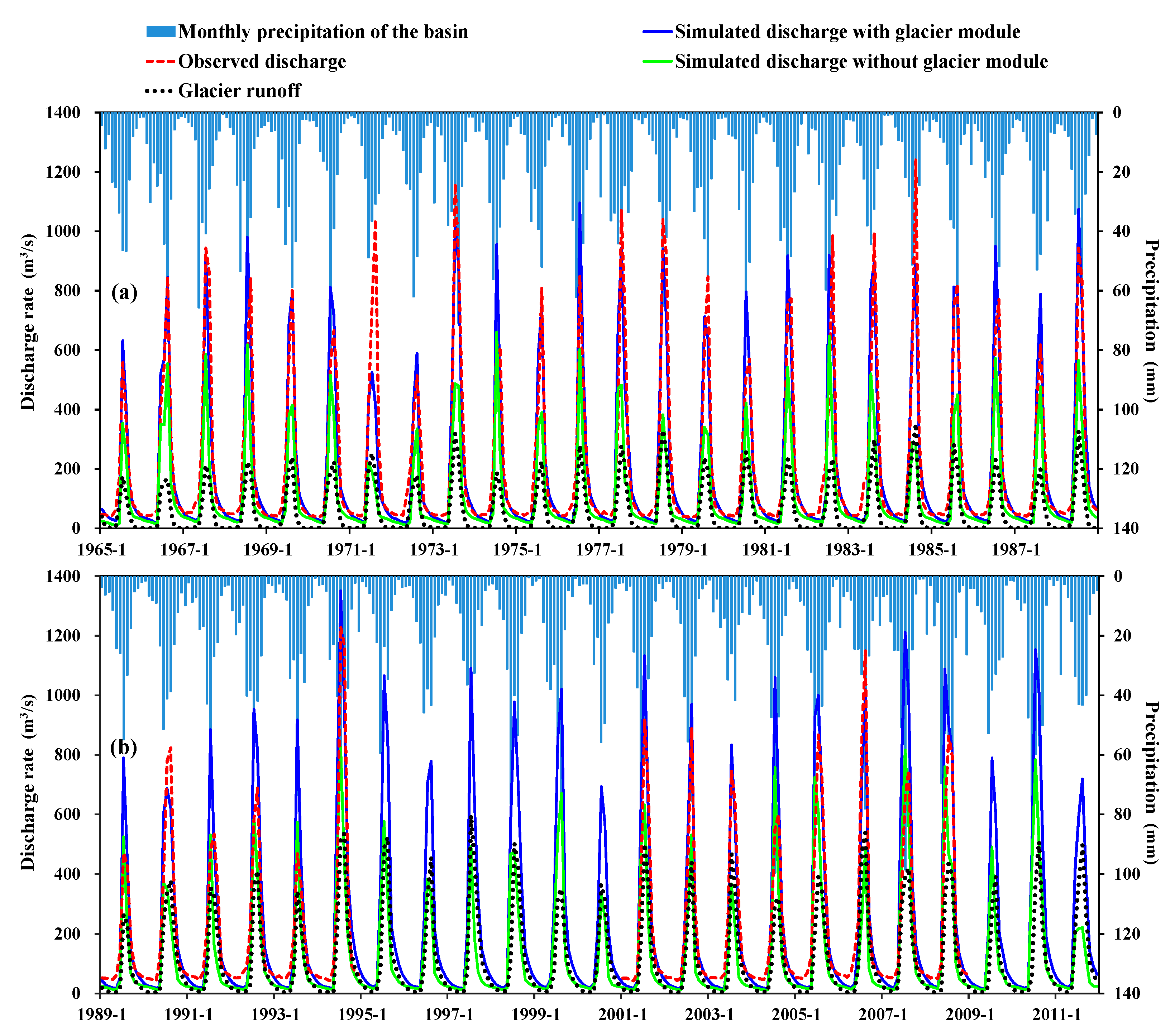
3.2. Model Performance

The statistical performance indices, NSE, RSR, and PBIAS, were employed to compare the simulated and measured monthly discharge values (

Table 3. Monthly streamflow (m³·s⁻¹) calibration and validation results for Yarkant River Basin (YRB), Northwest China. NSE: Nash–Sutcliff Efficiency; RSR: Root mean square error-observations standard deviation ratio; PBIAS: percentage bias.

Periods	NSE	RSR	PBIAS (%)
Calibration (January 1965–December 1988)	0.86	0.37	−4.51
Validation (January 1989–December 2011)	0.82	0.42	2.38
Overall (January 1965–December 2011)	0.85	0.39	−1.75

) including the calibration, validation, and overall periods. The two ‘warm-up periods’ in the calibration and validation periods were excluded from any statistical analyses.

Table 3 shows that the simulation results of the calibration period were slightly better than the results of the validation period, however, the results of both periods were ‘very good’ as rated following the rules given in Moriasi et al. [67]. In particular, the PBIAS index seemed to suggest that streamflow was slightly underestimated during the calibration period, and slightly overestimated in the validation period. From the statistical indices for the long time-series (i.e., the overall period), we show that the model achieved a ‘very good’ result, and that the streamflow was underestimated only by a small margin (i.e., 1.75%). In fact, the work of Peng and Xu [70] simulated streamflow in the Tarim River basin (including Aksu, Yarkant, and Hotan River basins) by using a modified semi-distributed monthly water balance model, to attain an NSE value between 0.60 and 0.69, and a relative error between −19% and 19%. According to the value of their NSE and PBIAS (which is a similar metric to their relative error), the results of our study can be considered as relatively better.

The monthly discharge curves based on the simulated and measured data in the calibration and validation periods (Figure 4), demonstrate a close alignment of the two discharge curves, except for several underestimated values in the month of July in 1971, 1977, 1978, 1984, and 2006. Correlations of monthly measured and simulated discharge were also analyzed by the seasons, as shown in Figure 5. The oblique line in this figure shows that the measured discharge in fact equals the simulated discharge value, where the optimal results are located on the oblique line. The points located above the line indicate some degree of overestimation, while the underestimated values are shown below the line. Hence, it is evident that the discharge values were underestimated in the spring season. In accordance with Figure 5a–d and the correlation coefficients (R²), we can infer that the results of the summer and autumn seasons were satisfactory, and that the model performances in winter and spring seasons were unsatisfactory.

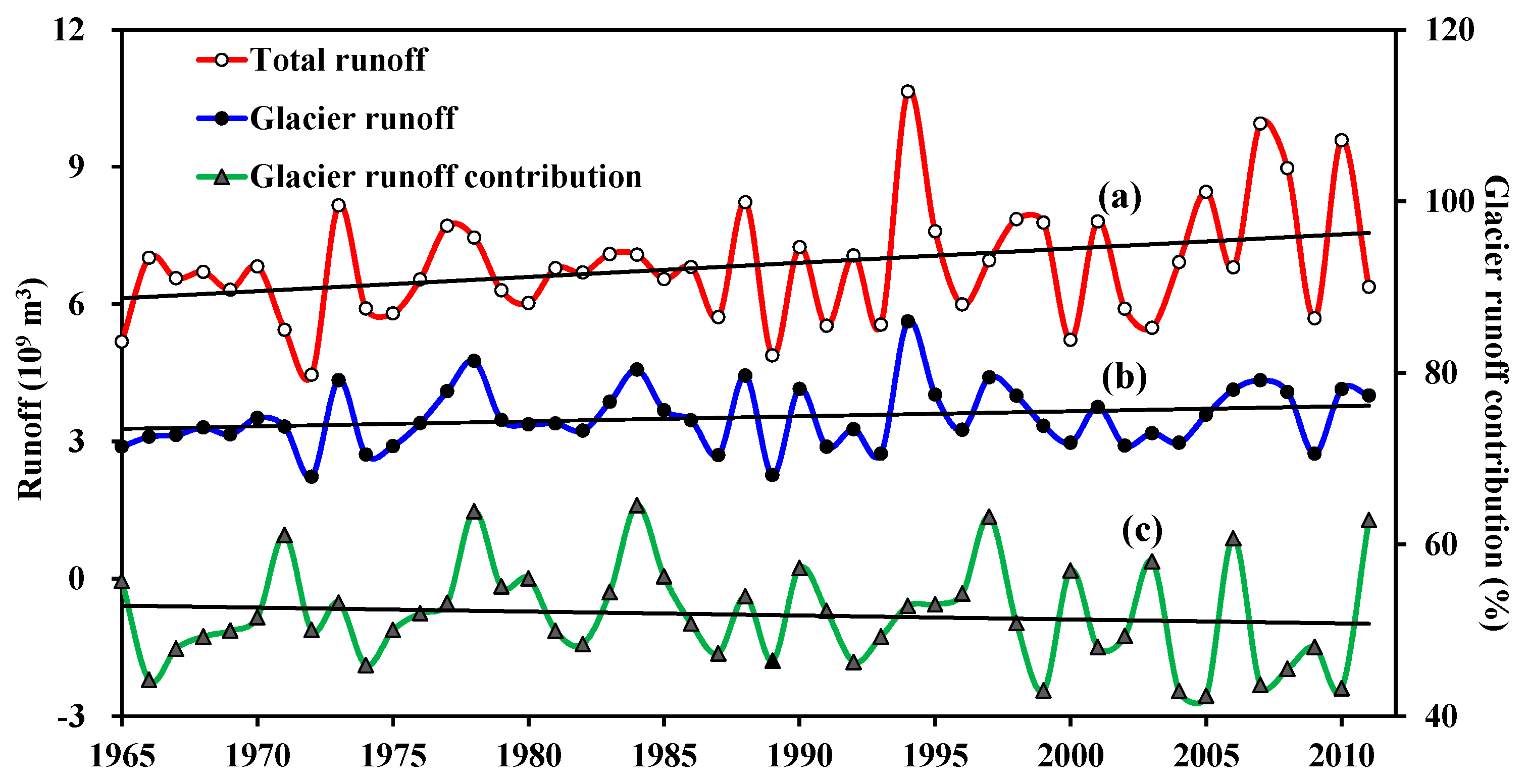
3.3. Annual Glacier Runoff Variation and Contribution

The simulated annual values as well as the linear trends of the total runoff, glacier runoff, and the glacier runoff contributions are shown in Figure 6. In accordance with this, it was clear that the total runoff exhbited a slowly increasing trend over the 50-year period of study. In the overall simulation period, the maximum and minimum runoff values of 10.64 × 10⁹ m³ and 4.456 × 10⁹ m³ occurred in the year 1994 and 1972, respectively. The multi-year average total runoff recorded a value of 6.84 × 10⁹ m³, with a rising trend of about 0.031 × 10⁹ m³·a⁻¹.

Figure 6 illustrates that the glacier runoff data also exhibited an increasing trend during the period of study. As such, the fluctuations of the glacier runoff hydrograph and the total runoff hydrograph were consistent with each other. The maximum and minimum simulated annual glacier runoff volumes were 5.621 × 10⁹ m³ and 2.230 × 10⁹ m³, respectively, and the multi-year average runoff was 3.527 × 10⁹ m³, contributing to 51.6% of the multi-year average total runoff. The increasing rate of glacier runoff, which was 0.011 × 10⁹ m³·a⁻¹, may be largely attributable due to the regional climate change factors that act to enhance the ablation of glaciers. The results showed that the total glacier area in YRB has decreased by 6.1% in the last forty years based on the results of remote sensing interpretations (e.g., [71]). In the past half century, however, the glacier runoff contribution to the total runoff volume appeared to be more or less consistent, from about 42.3% to 64.5% as shown in Figure 6c. Contrary to the increase in total and glacier runoff amounts, the glacier runoff contribution showed a slight decline by 0.046% a⁻¹. It is inferred that this may be caused by the different increasing rates of temperature and precipitation. This is in accordance with Chen et al. [72] in that the annual temperature showed a slightly increasing trend (0.24 °C) in the 1990s; however, the annual precipitation increased more significantly, rising by 20.7% between 1980s and the 1990s.

In an earlier study, Zhang et al. [21] employed a modified monthly degree-day model to estimate the glacier runoff in the Yarkant River Basin from 1961 to 2006. They reported that the total runoff in glacial areas exhibited an increasing rate of about 0.023 × 10⁹ m³·a⁻¹, similar to the result of our study. According to the study by Gao et al. [73], the glacier runoff accounted for 51.3% of the total runoff in the Yarkant River basin, which was nearly consistent with our calculated results that the glacier runoff contribution was 51.6% over the period from 1965 to 2011. Moreover, the impacts of temperature and precipitation on runoff in the Tarim River during the past 50 years indicated that both represented continuous increases of 0.04 °C 10 a⁻¹ and 11.2 mm 10 a⁻¹ for the Yarkant River basin, respectively [74], and meanwhile, the annual runoff exhibited an increasing trend. In this study, simulated annual and total precipitation increased by 10.5 mm 10 a⁻¹ and 0.045% 10 a⁻¹, respectively. According to the study in the Tarim River Basin [73], the river flow increased by 12.8% during the period from 1961 to 2006, of which approximately 1.8% was contributed by the increases in precipitation, and the others amounting to 11.0% originated from the glacier runoffs. That means that the increased glacier runoff accounted for as much as 85.7% of the increased river flows. Moreover, it is conceivable that the increased glacier runoff was caused by the increase of temperature.

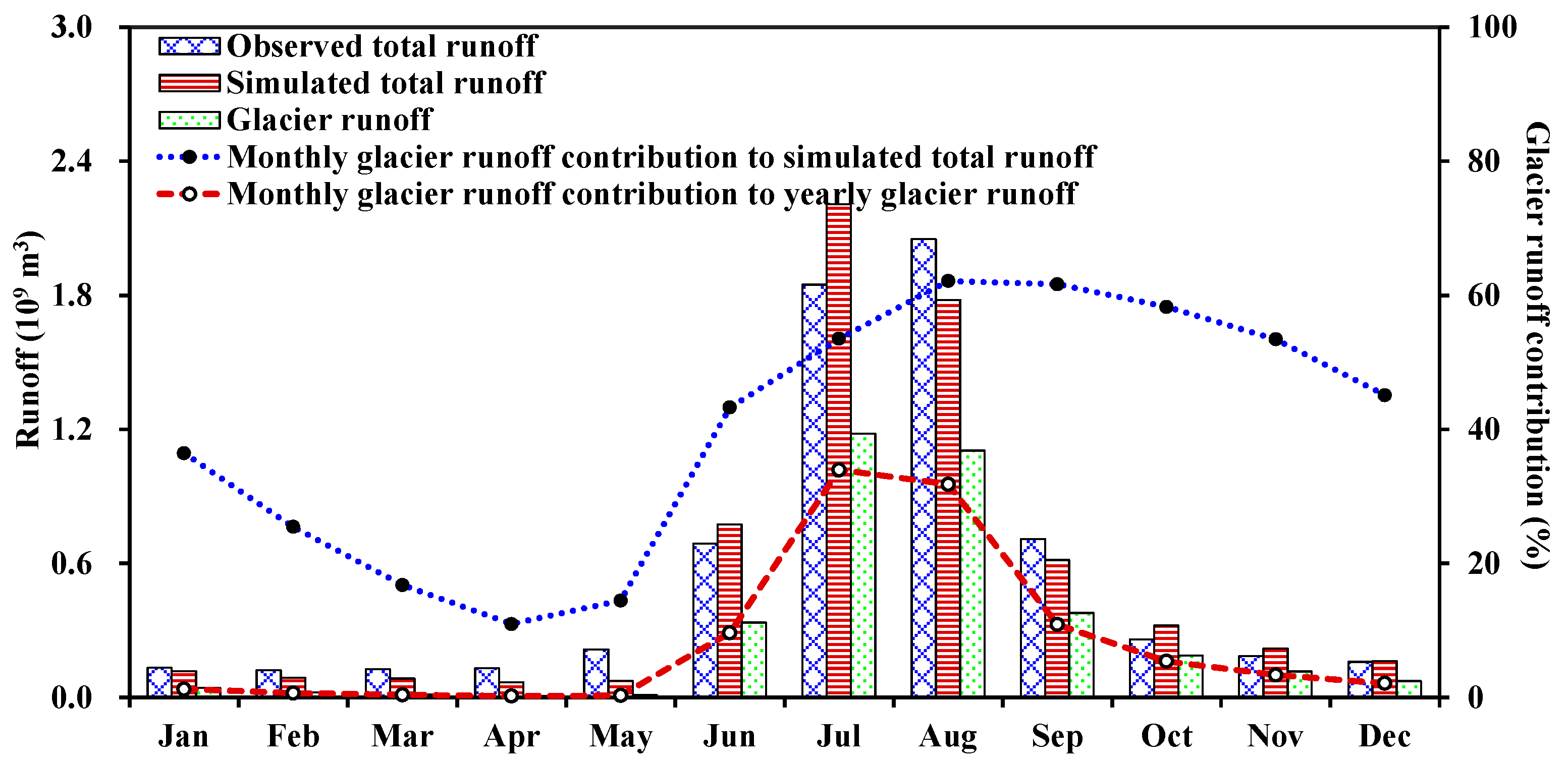
3.4. Multi-Year Monthly Average Glacier Runoff Contribution

The multi-year (1965–2011) monthly average measured runoff, simulated runoff, glacier runoff, and monthly glacier runoff contribution to annual glacier runoff are plotted in Figure 7. The monthly glacier runoff contribution to the monthly simulated total runoff ranged from 11.0% to 62.1%, with a minimum in April and a maximum in August. The value of the glacier runoff contribution gradually increased from April to August along with the rising temperatures, as shown in the monthly glacier runoff contribution to annual glacier runoff line chart. However, the monthly glacier runoff contribution continuously decreased until the April of the next year. Glacier runoff from January to May was almost negligible, amounting to only 0.099 × 10⁹ m³ in total, and accounted for only 2.8% of the annual glacier runoff. It is important to also note that the glacier runoff mainly occurred from the months of June to September during an average year, with 86.3% of the annual glacier runoff accounted for by 9.6% in June, 34.0% in July, 31.8% in August, and 10.9% in September.

The seasonal contribution of glacier runoff is known to significantly affect the regional water supply, especially in regions of High Asia [75]. Indeed, the work of Schaner et al. [13] produced global estimations of the monthly glacier runoff contribution to the total streamflow, and indicated that the maximum monthly contribution of glacier runoff was larger than 50% in the YRB. In our study, we calculated the maximum monthly contribution as about 62.1% in August. In the study of seasonal melt contributions of glacierized watersheds that originated in the Canadian Rocky Mountains [76], the results found that the glacier runoff contribution in July to September ranged from 73% to 83% for their watersheds, with a greater than 10% glacierized area; however, in our study, the glacierized area accounted for 12.6% of the glacier runoff contribution in July and 76.6% in September. We also calculated that the greatest glacier contributions that were in July and August, with estimations of 34.0% and 31.8%, respectively. However, a previous study [32] performed in the Mica basin (i.e., 5% glacier covered) showed that the greatest contributions were about 25% in August and 35% in September. These differences might be caused by the different geographic locations between the previous and our study (i.e., the Mica basin is further north of the YRB region).

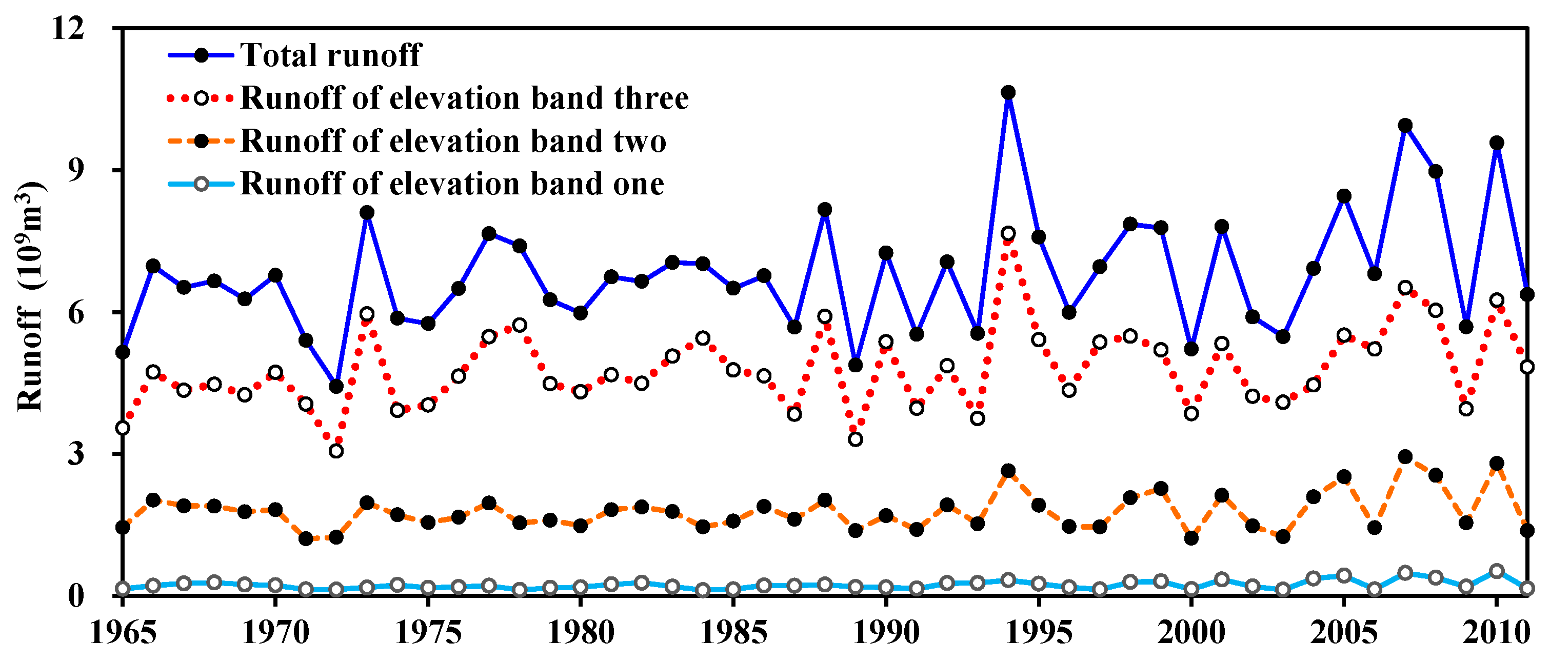
3.5. Glacier Runoff Contribution of Different Elevation Bands

In this paper, we divided the study area into three elevation bands using the 4000-m and 5000-m contour lines, as shown in Figure 8. The percentage areas of elevation from band one to three were 30.2%, 35.1%, and 34.7%, respectively. According to the first CGI, the glacier coverage was only 0.89 km² in elevation band one, which could be neglected when statistical analysis was performed according by the different elevation bands. However, the glacier coverage was 630.52 km² in elevation band two, accounting for an elevation band area and total glacier area of 3.9% and 32.53%, respectively, while the glacier coverage was 5263.45 km², accounting for 32.5% of the area within elevation band three and 89.3% of the total glacier area. Annual runoffs from the three elevation bands are shown in Figure 9. It was evident that the landscape that was lower than 4000 m hardly generated any runoff and the landscape higher than 5000 m was the main area generating the majority of the runoff volume. As determined from the simulated results, the multi-year average runoff contribution for the three elevation bands to the total runoff was about 3.3%, 26.2%, and 70.5% in elevation bands one, two and three, respectively, among which the glacier runoff contribution to the total runoff was about 5.2% and 46.4% in elevation bands two and three, respectively.

In context of the present research, quantifying the spatial and temporal contribution of glacier runoff has contributed to an improved understanding of streamflow generation processes within the alpine mountainous watersheds [25]. However, it should be noted that there were seemingly no prior studies that discussed the spatial hydrological responses in the YRB, except for the several temporal-related discussions (e.g., [77,78]). Therefore, in this sub-section of our simulation results, we calculated the spatial and annual contribution of different elevation bands to total runoff and glacier runoff based only on the simulated results because of the lack of observed data.

4. Summary

In this study, a glacial module based on the enhanced temperature-index approach was successfully incorporated into the Soil and Water Assessment Tool (SWAT) model to quantify the spatial and temporal contribution of glacier runoff to the watershed discharge in the Yarkant River Basin. In general, taking into account the glacial processes in the simulation model, the results closely matched the observed discharge data, indicating that the performance of the model was very good.

In accordance with the present results, over the last 50 years, the total discharge in the Yarkant River Basin has shown an increasing trend. Although the glaciers accounted for only 12.6% of the watershed drainage area, the contribution of annual average glacier runoff to streamflow was more than 50%. Meanwhile, the runoff volume of the Yarkant River Basin mainly originated from the high elevation regions above 5000 m a.s.l. and this accounted for more than 70% of the total runoff volume.

In summary, it is assertained that large watersheds and long-term glacier hydrological processes in the cold alpine regions are significant under the influence of climate change. Therefore, the simulation approach presented in this paper can likely be used to effectively help hydrologists in modeling large glaciated watersheds around the world, especially in data-scarce regions where observation records are relatively limited.

References

1. Morán-Tejeda, E.; Zabalza, J.; Rahman, K.; Gago-Silva, A.; López-Moreno, J.I.; Vicente-Serrano, S.; Lehmann, A.; Tague, C.L.; Beniston, M. Hydrological impacts of climate and land-use changes in a mountain watershed: Uncertainty estimation based on model comparison. Ecohydrology 2014, 8, 1396–1416. [Google Scholar] [CrossRef]
2. Ivy-Ochs, S. Glacier variations in the European Alps at the end of the last glaciation. Cuad. Investig. Geogr. 2015, 41, 295. [Google Scholar] [CrossRef]
3. Fischer, A. Glaciers and climate change: Interpretation of 50 years of direct mass balance of hintereisferner. Glob. Planet. Chang. 2010, 71, 13–26. [Google Scholar] [CrossRef]
4. Immerzeel, W.W.; van Beek, L.P.; Bierkens, M.F. Climate change will affect the asian water towers. Science 2010, 328, 1382–1385. [Google Scholar] [CrossRef] [PubMed]
5. Huss, M.; Farinotti, D.; Bauder, A.; Funk, M. Modelling runoff from highly glacierized alpine drainage basins in a changing climate. Hydrol. Process. 2008, 22, 3888–3902. [Google Scholar] [CrossRef]
6. Piao, S.; Ciais, P.; Huang, Y.; Shen, Z.; Peng, S.; Li, J.; Zhou, L.; Liu, H.; Ma, Y.; Ding, Y.; et al. The impacts of climate change on water resources and agriculture in China. Nature 2010, 467, 43–51. [Google Scholar] [CrossRef] [PubMed]
7. Feng, Q.; Miao, Z.; Li, Z.; Li, J.; Si, J.; S, Y.; Chang, Z. Public perception of an ecological rehabilitation project in inland river basins in northern China: Success or failure. Environ. Res. 2015, 139, 20–30. [Google Scholar] [CrossRef] [PubMed]
8. Oliva, M.; Antoniades, D.; Giralt, S.; Granados, I.; Pla-Rabes, S.; Toro, M.; Liu, E.J.; Sanjurjo, J.; Vieira, G. The holocene deglaciation of the Byers Peninsula (Livingston Island, Antarctica) based on the dating of lake sedimentary records. Geomorphology 2016, 261, 89–102. [Google Scholar] [CrossRef]
9. Huss, M. Present and future contribution of glacier storage change to runoff from macroscale drainage basins in Europe. Water Resour. Res. 2011, 47, W07511. [Google Scholar] [CrossRef]
10. Baraer, M.; Mark, B.G.; McKenzie, J.M.; Condom, T.; Bury, J.; Huh, K.-I.; Portocarrero, C.; Gómez, J.; Rathay, S. Glacier recession and water resources in Peru’s Cordillera Blanca. J. Glaciol. 2012, 58, 134–150. [Google Scholar] [CrossRef]
11. Pellicciotti, F.; Buergi, C.; Immerzeel, W.W.; Konz, M.; Shrestha, A.B. Challenges and uncertainties in hydrological modeling of remote Hindu Kush–Karakoram–Himalayan (HKH) basins: Suggestions for calibration strategies. Mt. Res. Dev. 2012, 32, 39–50. [Google Scholar] [CrossRef]
12. Feng, Q.; Wen, X.H.; Li, J.G. Wavelet analysis-support vector machine coupled models for monthly rainfall forecasting in arid regions. Water Resour. Manag. 2015, 29, 1049–1065. [Google Scholar] [CrossRef]
13. Schaner, N.; Voisin, N.; Nijssen, B.; Lettenmaier, D.P. The contribution of glacier melt to streamflow. Environ. Res. Lett. 2012, 7, 034029. [Google Scholar] [CrossRef]
14. Yin, Z.L.; Feng, Q.; Zou, S.B.; Yang, L.S. Assessing variation in water balance components in mountaious inland river basin experiencing climate change. Water 2016, 8, 472. [Google Scholar] [CrossRef]
15. Koboltschnig, G.R.; Schöner, W.; Zappa, M.; Kroisleitner, C.; Holzmann, H. Runoff modelling of the glacierized alpine upper Salzach Basin (Austria): Multi-criteria result validation. Hydrol. Process. 2008, 22, 3950–3964. [Google Scholar] [CrossRef]
16. Moors, E.J.; Groot, A.; Biemans, H.; van Scheltinga, C.T.; Siderius, C.; Stoffel, M.; Huggel, C.; Wiltshire, A.; Mathison, C.; Ridley, J.; et al. Adaptation to changing water resources in the Ganges Basin, northern India. Environ. Sci. Policy 2011, 14, 758–769. [Google Scholar] [CrossRef]
17. Bolch, T.; Kulkarni, A.; Kaab, A.; Huggel, C.; Paul, F.; Cogley, J.G.; Frey, H.; Kargel, J.S.; Fujita, K.; Scheel, M.; et al. The state and fate of Himalayan glaciers. Science 2012, 336, 310–314. [Google Scholar] [CrossRef] [PubMed] [Green Version]
18. Oliva, M.; Serrano, E.; Gómez-Ortiz, A.; González-Amuchastegui, M.J.; Nieuwendam, A.; Palacios, D.; Pérez-Alberti, A.; Pellitero-Ondicol, R.; Ruiz-Fernández, J.; Valcárcel, M.; et al. Spatial and temporal variability of periglaciation of the Iberian Peninsula. Quat. Sci. Rev. 2016, 137, 176–199. [Google Scholar] [CrossRef]
19. Kaser, G.; Grosshauser, M.; Marzeion, B. Contribution potential of glaciers to water availability in different climate regimes. Proc. Natl. Acad. Sci. USA 2010, 107, 20223–20227. [Google Scholar] [CrossRef] [PubMed]
20. Gascoin, S.; Kinnard, C.; Ponce, R.; Lhermitte, S.; MacDonell, S.; Rabatel, A. Glacier contribution to streamflow in two headwaters of the Huasco river, Dry Andes of Chile. Cryosphere 2011, 5, 1099–1113. [Google Scholar] [CrossRef] [Green Version]
21. Zhang, S.; Gao, X.; Ye, B.; Zhang, X.; Hagemann, S. A modified monthly degree-day model for evaluating glacier runoff changes in China. Part II: Application. Hydrol. Process. 2012, 26, 1697–1706. [Google Scholar] [CrossRef]
22. Liu, S.Y.; Zhang, Y.; Zhang, Y.S.; Ding, Y.J. Estimation of glacier runoff and future trends in the Yangtze River source region, China. J. Glaciol. 2009, 55, 353–362. [Google Scholar]
23. Kong, Y.; Pang, Z. Evaluating the sensitivity of glacier rivers to climate change based on hydrograph separation of discharge. J. Hydrol. 2012, 434–435, 121–129. [Google Scholar] [CrossRef]
24. Li, Z.X.; Feng, Q.; Liu, W.; Wang, T.T.; Cheng, A.F.; Gao, Y.; Guo, X.Y.; Pan, Y.H.; Li, J.G.; Guo, R. Study on the contribution of cryosphere to runoff in the cold alpine basin: A case study of Hulugou River Basin in the Qilian Mountains. Glob. Planet. Chang. 2014, 122, 345–361. [Google Scholar]
25. Rahman, K.; Besacier-Monbertrand, A.L.; Castella, E.; Lods-Crozet, B.; Ilg, C.; Beguin, O. Quantification of the daily dynamics of streamflow components in a small alpine watershed in Switzerland using end member mixing analysis. Environ. Earth Sci. 2015, 74, 1–11. [Google Scholar] [CrossRef]
26. Nolin, A.W.; Phillippe, J.; Jefferson, A.; Lewis, S.L. Present-day and future contributions of glacier runoff to summertime flows in a Pacific Northwest watershed: Implications for water resources. Water. Resour. Res. 2010, 46, W12509. [Google Scholar] [CrossRef]
27. Prasch, M.; Mauser, W.; Weber, M. Quantifying present and future glacier melt-water contribution to runoff in a central Himalayan river basin. Cryosphere 2013, 7, 889–904. [Google Scholar] [CrossRef]
28. Boscarello, L.; Ravazzani, G.; Rabuffetti, D.; Mancini, M. Integrating glaciers raster-based modelling in large catchments hydrological balance: The Rhone case study. Hydrol. Process. 2014, 28, 496–508. [Google Scholar] [CrossRef]
29. La Frenierre, J.; Mark, B.G. A review of methods for estimating the contribution of glacial meltwater to total watershed discharge. Prog. Phys. Geogr. 2014, 38, 173–200. [Google Scholar] [CrossRef]
30. Debele, B.; Srinivasan, R.; Gosain, A.K. Comparison of process-based and temperature-index snowmelt modeling in SWAT. Water Resour. Manag. 2009, 24, 1065–1088. [Google Scholar] [CrossRef]
31. Gao, H.; He, X.; Ye, B.; Pu, J. Modeling the runoff and glacier mass balance in a small watershed on the central Tibetan Plateau, China, from 1955 to 2008. Hydrol. Process. 2012, 26, 1593–1603. [Google Scholar] [CrossRef]
32. Jost, G.; Moore, R.D.; Menounos, B.; Wheate, R. Quantifying the contribution of glacier runoff to streamflow in the upper Columbia River Basin, Canada. Hydrol. Earth Syst. Sci. 2012, 16, 849–860. [Google Scholar] [CrossRef] [Green Version]
33. Farinotti, D.; Usselmann, S.; Huss, M.; Bauder, A.; Funk, M. Runoff evolution in the Swiss Alps: Projections for selected high-alpine catchments based on ensembles scenarios. Hydrol. Process. 2012, 26, 1909–1924. [Google Scholar] [CrossRef]
34. Gabbi, J.; Farinotti, D.; Bauder, A.; Maurer, H. Ice volume distribution and implications on runoff projections in a glacierized catchment. Hydrol. Earth Syst. Sci. 2012, 16, 4543–4556. [Google Scholar] [CrossRef] [Green Version]
35. Nepal, S.; Krause, P.; Flügel, W.A.; Fink, M.; Fischer, C. Understanding the hydrological system dynamics of a glaciated alpine catchment in the Himalayan region using the J2000 hydrological model. Hydrol. Process. 2014, 28, 1329–1344. [Google Scholar] [CrossRef]
36. Verbunt, M.; Gurtz, J.; Jasper, K.; Lang, H.; Warmerdam, P.; Zappa, M. The hydrological role of snow and glaciers in alpine river basins and their distributed modeling. J. Hydrol. 2003, 282, 36–55. [Google Scholar] [CrossRef]
37. Finger, D.; Heinrich, G.; Gobiet, A.; Bauder, A. Projections of future water resources and their uncertainty in a glacierized catchment in the Swiss Alps and the subsequent effects on hydropower production during the 21st century. Water Resour. Res. 2012, 48, W02521. [Google Scholar] [CrossRef]
38. Luo, Y.; Arnold, J.; Liu, S.; Wang, X.; Chen, X. Inclusion of glacier processes for distributed hydrological modeling at basin scale with application to a watershed in Tianshan Mountains, northwest China. J. Hydrol. 2013, 477, 72–85. [Google Scholar] [CrossRef]
39. Rahman, K.; Maringanti, C.; Beniston, M.; Widmer, F.; Abbaspour, K.; Lehmann, A. Streamflow modeling in a highly managed mountainous glacier watershed using SWAT: The upper Rhone river watershed case in Switzerland. Water Resour. Manag. 2012, 27, 323–339. [Google Scholar] [CrossRef]
40. Hock, R. Temperature index melt modelling in mountain areas. J. Hydrol. 2003, 282, 104–115. [Google Scholar] [CrossRef]
41. Hock, R. A distributed temperature-index ice- and snowmelt model including potential direct solar radiation. J. Glaciol. 1999, 45, 101–111. [Google Scholar] [CrossRef]
42. Pellicciotti, F.; Brock, B.; Strasser, U.; Burlando, P.; Funk, M.; Corripio, J. An enhanced temperature-index glacier melt model including the shortwave radiation balance: Development and testing for Haut Glacier d’Arolla, Switzerland. J. Glaciol. 2005, 51, 573–587. [Google Scholar] [CrossRef]
43. Zappa, M.; Pos, F.; Strasser, U.; Warmerdam, P.M.M.; Gurtz, J. Seasonal water balance of an alpine catchment as evaluated by different methods for spatially distributed snowmelt modelling. Hydrol. Res. 2003, 34, 179–202. [Google Scholar]
44. Rahman, K.; Etienne, C.; Gago-Silva, A.; Maringanti, C.; Beniston, M.; Lehmann, A. Streamflow response to regional climate model output in the mountainous watershed: A case study from the Swiss Alps. Environ. Earth Sci. 2014, 72, 4357–4369. [Google Scholar] [CrossRef]
45. Radić, V.; Hock, R. Glaciers in the earth’s hydrological cycle: Assessments of glacier mass and runoff changes on global and regional scales. Surv. Geophys. 2013, 35, 813–837. [Google Scholar] [CrossRef]
46. Wang, X.; Sun, L.; Zhang, Y.; Luo, Y. Rationalization of altitudinal precipitation profiles in a data-scarce glacierized watershed simulation in the Karakoram. Water 2016, 8, 186. [Google Scholar] [CrossRef]
47. Huang, S.; Krysanova, V.; Zhai, J.; Su, B. Impact of intensive irrigation activities on river discharge under agricultural scenarios in the semi-arid Aksu River Basin, northwest China. Water Resour. Manag. 2015, 29, 1–15. [Google Scholar] [CrossRef]
48. Chen, Y.; Xu, C.; Chen, Y.; Li, W.; Liu, J. Response of glacial-lake outburst floods to climate change in the Yarkant River Basin on northern slope of Karakoram Mountains, China. Quatern. Int. 2010, 226, 75–81. [Google Scholar] [CrossRef]
49. Liu, S.Y.; Yao, X.J.; Guo, W.Q.; Xu, J.L.; Shangguan, D.H.; Wei, J.F.; Bao, W.J.; Wu, L.Z. The contemporary glaciers in China based on the Second Chinese Glacier Inventory. Acta Geogr. Sin. 2015, 70, 3–16. (In Chinese) [Google Scholar]
50. Yang, H.A.; An, R.Z. Glacier Inventory of China, V: Karakorum Mountains (Drainage Basin of the Yarkant River); Science Press: Bejing, China, 1989. [Google Scholar]
51. Zhang, X.S.; Zhou, Y.C. Study on the Glacier Lake Outburst Floods of the Yarkant River, Karakorum Mountains; Science Press: Beijing, China, 1990. [Google Scholar]
52. Liu, J.; Liu, T.; Bao, A.; De Maeyer, P.; Kurban, A.; Chen, X. Response of hydrological processes to input data in high alpine catchment: An assessment of the Yarkant River Basin in China. Water 2016, 8, 181. [Google Scholar] [CrossRef]
53. Xu, Y.; Gao, X.; Shen, Y.; Xu, C.; Shi, Y.; Giorgi, F. A daily temperature dataset over China and its application in validating a RCM simulation. Adv. Atmos. Sci. 2009, 26, 763–772. [Google Scholar] [CrossRef]
54. Zhao, Y.F.; Zhu, J. Assessing quality of grid daily precipitation datasets in China in recent 50 years. Plateau Meteorol. 2015, 34, 50–58. (In Chinese) [Google Scholar]
55. Guo, D.; Wang, H. Simulation of permafrost and seasonally frozen ground conditions on the Tibetan Plateau, 1981–2010. J. Geophys. Res. Atmos. 2013, 118, 5216–5230. [Google Scholar] [CrossRef]
56. Arnold, J.G.; Srinivasan, R.; Williams, J.R. Large area hydrologic modeling and assessment. Part I: Model development. J. Am. Water Resour. Assoc. 1998, 34, 73–89. [Google Scholar] [CrossRef]
57. Neitsch, S.L.; Arnold, J.G.; Kiniry, J.R.; Williams, J.R. Soil and Water Assessment Tool Theoretical Documentation: Version 2005; USDA-ARS Grassland, Soil and Water Research Laboratory: Temple, TX, USA, 2005. [Google Scholar]
58. Gassman, P.W.; Reyes, M.R.; Green, C.H.; Arnold, J.G. The soil and water assessment tool: Historical development, applications, and future research directions. Trans. Asabe 2007, 50, 1211–1250. [Google Scholar] [CrossRef]
59. Wang, X.; Melesse, A.M. Evaluation of the SWAT model’s snowmelt hydrology in a northwestern minnesota watershed. Trans. ASABE 2005, 48, 1359–1376. [Google Scholar] [CrossRef]
60. Zhang, X.; Srinivasan, R.; Debele, B.; Hao, F. Runoff simulation of the headwaters of the Yellow River using the SWAT model with three snowmelt algorithms. J. Am. Water Resour. Assoc. 2008, 44, 48–61. [Google Scholar] [CrossRef]
61. Zhang, W.; Zha, X.; Li, J.; Liang, W.; Ma, Y.; Fan, D.; Li, S. Spatiotemporal change of blue water and green water resources in the headwater of Yellow River Basin, China. Water Resour. Manag. 2014, 28, 4715–4732. [Google Scholar] [CrossRef]
62. Zhang, Y.; Fujita, K.; Liu, S.; Liu, Q.; Nuimura, T. Distribution of debris thickness and its effect on ice melt at Hiluogou glacier, southeastern Tibetan Plateau, using in situ surveys and ASTER imagery. J. Glaciol. 2011, 57, 1147–1157. [Google Scholar] [CrossRef]
63. Garnier, B.J.; Ohmura, A. A method of calculating the direct shortwave radiation income of slopes. J. Appl. Meteorol. 1968, 7, 796–800. [Google Scholar] [CrossRef]
64. Jiang, X.; Wang, N.; He, J.; Wu, X.; Song, G. A distributed surface energy and mass balance model and its application to a mountain glacier in China. Chin. Sci. Bull. 2010, 55, 2079–2087. [Google Scholar] [CrossRef]
65. Liu, S.Y.; Sun, W.X.; Shen, Y.P.; Li, G. Glacier changes since the Little Ice Age maximum in the western Qilian Shan, northwest China, and consequences of glacier runoff for water supply. J. Glaciol. 2003, 49, 117–124. [Google Scholar]
66. Meier, M.F.; Bahr, D.B. Counting Glaciers: Use of Scaling Methods to Estimate the Number and Size Distribution of the Glaciers of the World; U.S. Army: Hanover, NH, USA, 1996. [Google Scholar]
67. Moriasi, D.N.; Arnold, J.G.; Van Liew, M.W.; Bingner, R.L.; Harmel, R.D.; Veith, T.L. Model evaluation guidelines for systematic quantification of accuracy in watershed simulations. Trans. ASABE 2007, 50, 885–900. [Google Scholar] [CrossRef]
68. Zhang, Y.; Liu, S.; Ding, Y. Observed degree-day factors and their spatial variation on glaciers in western China. Ann. Glaciol. 2006, 43, 301–306. [Google Scholar] [CrossRef]
69. Zhang, Y.; Liu, S.; Xu, J.; Shangguan, D. Glacier change and glacier runoff variation in the Tuotuo River basin, the source region of Yangtze River in western China. Environ. Geol. 2008, 56, 59–68. [Google Scholar] [CrossRef]
70. Peng, D.Z.; Xu, Z.X. Simulating the impact of climate change on streamflow in the Tarim River Basin by using a modified semi-distributed monthly water balance model. Hydrol. Process. 2010, 24, 209–216. [Google Scholar] [CrossRef]
71. Shangguan, D.; Liu, S.; Ding, Y.; Ding, L.; Xu, J.; Jing, L. Glacier changes during the last forty years in the Tarim interior River Basin, northwest China. Prog. Nat. Sci. 2009, 19, 727–732. [Google Scholar] [CrossRef]
72. Chen, Y.N.; Xu, C.C.; Hao, X.M.; Li, W.H.; Chen, Y.P.; Zhu, C.G.; Ye, Z.X. Fifty-year climate change and its effect on annual runoff in the Tarim River Basin, China. Quat. Int. 2009, 208, 53–61. [Google Scholar]
73. Gao, X.; Ye, B.; Zhang, S.; Qiao, C.; Zhang, X. Glacier runoff variation and its influence on river runoff during 1961–2006 in the Tarim River Basin, China. Sci. China Earth Sci. 2010, 53, 880–891. [Google Scholar] [CrossRef]
74. Fan, Y.; Chen, Y.; Li, W.; Wang, H.; Li, X. Impacts of temperature and precipitation on runoff in the Tarim River during the past 50 years. J. Arid Land 2011, 3, 220–230. [Google Scholar] [CrossRef]
75. Hock, R. Glacier melt: A review of processes and their modelling. Prog. Phys. Geogr. 2002, 27, 362–391. [Google Scholar] [CrossRef]
76. Comeau, L.E.L.; Pietroniro, A.; Demuth, M.N. Glacier contribution to the North and South Saskatchewan Rivers. Hydrol. Process. 2009, 23, 2640–2653. [Google Scholar] [CrossRef]
77. Ling, H.; Xu, H.; Fu, J. Changes in intra-annual runoff and its response to climate change and human activities in the headstream areas of the Tarim River Basin, China. Quat. Int. 2014, 336, 158–170. [Google Scholar] [CrossRef]
78. Xu, Z.; Liu, Z.; Fu, G.; Chen, Y. Trends of major hydroclimatic variables in the Tarim River Basin during the past 50 years. J. Arid Environ. 2010, 74, 256–267. [Google Scholar] [CrossRef]
Figure 1. Location of the meteorological and hydrological sites with the grid points. GCI: China Glacier Inventory.
Water 09 00159 g001
Figure 2. Comparison of the meteorological station-based air temperature and precipitation with the nearest grid data; (a) mean monthly air temperature; (b) mean monthly precipitation; (c) correlation between the meteorological station monthly air temperature and that of the nearest grid data; (d) correlation between the meteorological station monthly precipitation and that of the nearest grid data. R2: coefficient of determination.
Water 09 00159 g002
Figure 3. The spatial and temporal variation of ice melt factor; (a) The spatial distribution of ice melt factor for the 182nd day in a year; (b) The partial enlarged drawing; (c) The temporal variation of ice melt factor for the representative dot in a year.
Water 09 00159 g003
Figure 4. Comparison of simulated versus measured monthly streamflow processes; (a) Calibration period: January 1965 to December 1988; (b) Validation period: January 1989 to December 2011; with measured data missing in the periods from January 1995 to December 2000, and January 2009 to December 2011.
Water 09 00159 g004
Figure 5. Coefficient of determination (R2) for overall period at seasonal statistics by monthly results; (a) Spring (March–May); (b) Summer (June–August); (c) Autumn (September–November); (d) Winter (December–February).
Water 09 00159 g005
Figure 6. Simulated annual total runoff, glacier runoff, glacier runoff contribution, as well as their variation trends.
Water 09 00159 g006
Figure 7. Multi-year monthly average observed and simulated total runoff, glacier runoff as well as its monthly contributions.
Water 09 00159 g007
Figure 8. Elevation bands of the YRB.
Water 09 00159 g008
Figure 9. Annual runoff of different elevation bands.
Water 09 00159 g009