Statistical Dependence of Pipe Breaks on Explanatory Variables

Abstract

Aging infrastructure is the main challenge currently faced by water suppliers. Estimation of assets lifetime requires reliable criteria to plan assets repair and renewal strategies. To do so, pipe break prediction is one of the most important inputs. This paper analyzes the statistical dependence of pipe breaks on explanatory variables, determining their optimal combination and quantifying their influence on failure prediction accuracy. A large set of registered data from Madrid water supply network, managed by Canal de Isabel II, has been filtered, classified and studied. Several statistical Bayesian models have been built and validated from the available information with a technique that combines reference periods of time as well as geographical location. Statistical models of increasing complexity are built from zero up to five explanatory variables following two approaches: a set of independent variables or a combination of two joint variables plus an additional number of independent variables. With the aim of finding the variable combination that provides the most accurate prediction, models are compared following an objective validation procedure based on the model skill to predict the number of pipe breaks in a large set of geographical locations. As expected, model performance improves as the number of explanatory variables increases. However, the rate of improvement is not constant. Performance metrics improve significantly up to three variables, but the tendency is softened for higher order models, especially in trunk mains where performance is reduced. Slight differences are found between trunk mains and distribution lines when selecting the most influent variables and models.

1. Introduction

Aging infrastructure involves an increasing risk of failure in underground water pipes that have consequences in the quality of service provided to end-users. For developed countries, aging infrastructure is a current concern but it is likely to become an important issue worldwide in the future [1]. Water distribution networks are large scale systems which demand continuous improvements for their design optimization or to achieve appropriate levels of efficiency [2]. Likewise, increasing asset investment is required for rehabilitation or repairing to maintain the level of service. Service suppliers make remarkable efforts to establish suitable asset management policies in order to improve the decision making process while managing uncertainties for medium or long-term planning [3]. These tasks involve deep understanding of system performance, network deterioration processes and pipe failure mechanisms.

The development of water network models to foresee the system possible behavior contributes to an effective asset management. Indeed, some researchers are centered on determining an optimal pipe replacement strategy based on failure prediction models [4,5]. From this approach some studies identify the remaining service life as the period of time at the end of which a pipe stops providing the function it was designed for [6]. Over this period, communities would face increasing repair costs [7]. This way, different models to predict pipe failure have been developed in order to determine that period of time for programming not only preventive or proactive repair campaigns but also renewal programs. However, uncertainty related to the quality and the quantity of data needed to build the model also has to be faced.

Pipe failure models can be grouped as physically based models and statistical models [8]. While the first group aims to discover the physical mechanisms behind pipe breaks, statistical models are based on historical break data to identify break patterns in the water mains [9]. Models are also classified as deterministic or stochastic models [10]. In deterministic models the number of failures is calculated from mathematical functions based on explanatory variables but they need large series of known variables data. Meanwhile, stochastic models take into account the random nature of failures. They can be classified as: single-variate models and multivariate models. Multivariate models allow a better understanding of the influence of each parameter in failure occurrence but require fixing how the covariates act on the failure distribution. On the other hand, single-variate models require dividing the input data into homogeneous groups assuming a constant failure rate within the group.

Some research projects are being developed for a better understanding of the explanatory factors of bursts and failures. Condition assessment studies [11] are conducted to identify main variables related to the asset deterioration process. Effective decisions about the likelihood of failure and renewal planning are based on collection of information about asset condition, analysis of this information and ultimately transformation of this information into knowledge [12,13]. Condition assessment methods can be classified into direct and indirect methods [14]. Direct methods include automated/manual visual inspection, non-destructive testing and pipe sampling. Indirect methods include water audit, flow testing, and measurement of terrain resistivity to determine the risk of deterioration. However, all these techniques are quite expensive and uncertainties are still substantial.

Data quality becomes a key factor when building the pipe break predictive model because of the large data sets required to develop a reliable model and the uncertainties associated to the data record process [15,16,17,18]. Therefore, Bayesian analysis based on considering random variables and incorporating external information to build a probability distribution has been selected by several researches [19,20,21,22] as a good approach to describe the uncertainties in the model parameters.

In this regard, a model able to predict pipe failure should be built from reliable data in a robust manner. Based on this idea and in order to improve the understanding of failure processes, an accurate quantification of model and uncertainties in prediction has become a key problem [23,24].

Commonly, the occurrence of failures increases with the age of network elements [25]. However, while some components can be operative for longer periods than their design life, other younger elements present a high failure rate and need to be replaced soon [26]. This could be explained by the fact that failures in pipelines depend on many factors that are difficult to characterize quantitatively [27]. Assets aging involves its natural deterioration but there are some other drivers such as external corrosion, the amount of loading (pressure, and ground movement), the pipe length and diameter, the pipe material, the quality of installation and workmanship, and even the burst history itself that influences the failure process [28].

Structural deterioration of elements in water networks are usually produced by specific influencing factors related to environmental conditions and material characteristics [29]. Influencing variables are categorized as [30,31]: structural or physical variables, external or environmental variables, internal or hydraulic variables and maintenance variables. However, the influence of these factors on pipe breaks and the analysis of their capability to predict failures are not properly quantified.

The aim of the research reported in this paper is to evidence the statistical dependence of pipe breaks on explanatory variables. It is developed from a complete database of pipe failures where every failure at each element has been carefully registered along a four-year period (2010–2014). Such failure database has provided a great chance to develop a quantitative analysis of the influence of explanatory variables in the task of predicting failures by their appropriate combination. This results in an improvement of the models’ performance.

In the following section, this paper details the applied input data in terms of failure registration and pipe characteristics. Section 2.2 describes the methodology applied: selection of explanatory variables, description of the Bayesian analysis used, how the different models are built and finally the validation process of applied models. After the technique is described, results obtained for the Canal de Isabel II network (trunk mains and distribution lines) are explained in Section 3. Main findings obtained by direct comparison of the performance of the applied models to each of the networks are explained in Section 4. To conclude, the last section summarizes the main conclusions of the research in terms of pipe break dependence on explanatory variables and best combination of variables for pipe break prediction models.

2. Data and Methods

2.1. Data

Statistical dependence of explanatory variables on pipe breaks is analyzed with a large set of data recorded in the water supply network managed by Canal de Isabel II. Canal de Isabel II is the company commissioned for the integral water cycle in Madrid’s region. The urban water network managed by the company covers more than 8000 km² and supplies water to more than 177 municipalities. It is composed of a set of trunk mains and a set of distribution lines. The distribution lines are formed by more than 370,000 pipe segments with a total length of more than 14,000 km. The trunk mains are formed by close to 40,000 elements with more than 3000 km of total length. The present analysis is focused on the water supply networks (trunk mains and distribution pipes). Part of the assets managed by Canal de Isabel II, such as water treatment plants, pumping stations, water channels and service connections, are not considered in this study.

Canal de Isabel II records network data from every pipe segment and other elements such as age, material, diameter, and depth in its own geographic information system (GIS). Since 2004, the company has implemented a Sectorization Plan, with 779 hydraulic sectors already in service that enables a more accurate knowledge of network performance. Through the sectorization, much information about the pressure on each sector’s inlet is gathered with the monitoring system (SCADA). In addition, the entire network of Canal de Isabel II is incorporated into calibrated and bimonthly updated hydraulic models of system operation. Such mathematical models also provide hydraulic variables that were considered in the analysis. Representative pressure and velocity values (maximum, average and minimum) for each pipe segment of the network were taken into account in this research.

Moreover, a large series of system failures is recorded by the corresponding information management system (named GAYTA). That system incorporates a database of events related to breaks, leaks, water quality or low pressure problems, client claims and other relevant information communicated to Canal de Isabel II by any other stakeholder, works and operation activities carried out within the network as well as maintenance labors. For each of them, a set of parameters have been introduced in a database as well as the location, the municipality and the hydraulic sector where it is located. This study has been developed from failure records between 2011 and 2014. Complementary data regarding operational maneuvers in this period have been used to identify their influence on pipe failures.

The GAYTA database collected information of more than 433,000 system events in the considered period (2011–2014). Filtering techniques were applied to remove duplicated events and works from the input databases. This process is quite relevant when considering the events information registered in the corresponding information system. To do so the following filters were applied: firstly, we selected every event that was produced by any activity of the company. In a second filter those events out of the scope of the study were removed; this applies to service connections, valves, and other special devices reducing the set of data to 155,407 registers. The third filter only considers events related to breaks and leakages which reduced the number of events to 61,870. The fourth filter was applied to remove those events where the location is not properly identified and thus the failure cannot be assigned to a specific pipe segment. Similar filters were applied to every variable so as to remove all those pipe segments where the information set is not complete whether because of the parameters of the pipe itself or because the registered information in the events database is not complete. Finally, about 10,000 events were selected for analysis in the distribution lines and 410 events in the trunk mains.

The main parameters of the data used in this research are summarized in

Table 1. Analyzed data.

Category	Number of Components	2011	2012	2013	2014
		Events	Events	Events	Events
Distribution lines	373,113 (14,176 km)	1758	1773	1970	2237
Trunk mains	39,915 (3297 km)	94	78	74	79

.

Other sources of information were also used in this analysis; the geological characterization of the terrain was taken from geological maps developed by the Spanish Geologic and Mining Institute. Such maps were correlated with the GIS data so that a type of terrain was identified for each pipe segment of the network. Regarding land use, national data were also taken into account. The Land Use System Information (SIOSE) provides information about that characteristic considering several categories: artificial cover, crops, water surfaces, combined, infrastructure, etc. Each type of land cover has several subtypes depending on the application such as roads, railways, airports, commercial areas, industrial areas, etc. This information was synthetized for a detailed characterization of every pipe segment within the network.

By incorporating all this information to a certain methodology several predictive models can be proposed as described in the following section. Every source involves several variables that are incorporated in the study. From the Canal de Isabel II GIS: diameter, installation year, material and location are obtained. From the geographical referenced maps: terrain, land use and depth are taken. From the hydraulic models, maximum, average and minimum pressures as well as maximum, average and minimum velocity are calculated. From the operational and works database, hydraulic transient ratio is considered for every pipe by analyzing the relationship between system maneuvers at special network elements and their incidence in the rest of system components. The list of considered factors classified as physical, environmental or internal variables for each type of network is shown in

Table 2. Considered variables.

Type of Variable	Distribution Lines	Trunk Mains
Physical	Diameter	Diameter
Physical	Installation year	Installation year
Physical	Material	Material
Environmental	Terrain	-
Environmental	Land use	Land use
Environmental	Depth	Depth
Internal	Maximum pressure	Maximum pressure
Internal	Average pressure	Average pressure
Internal	Minimum pressure	Minimum pressure
Internal	Maximum velocity	Maximum velocity
Internal	Average velocity	Average velocity
Internal	Minimum velocity	Minimum velocity
Internal	Transient index	Transient index

.

Such large amount of information was compiled and classified to produce several predictive models incorporating different variables with the aim of identifying the most relevant variables in the failure phenomena.

2.2. Methodology

The analysis of all collected data is assessed in three steps: first, the explanatory variables that can influence the pipe break phenomena are selected; second, several predictive models with multiple variables combined in different manners are formed; and to conclude the analysis, the third step is to evaluate the results obtained for each of the proposed models in order to look for the best predictive option for distribution and for trunk mains.

2.2.1. Explanatory Variables Selection

The variable selection was done following a two-step approach. Firstly, a set of candidate variables were selected based on current state of the art. Variables taken from the literature include those usually related to pipe breaks: material, diameter and year of installation (pipe age). These three variables are considered principal variables in the analysis. A second group of variables was selected. In this case, their influence on break prediction is not that evident, thus they are considered as secondary variables. They were identified from a holistic point of view. Every considered variable is listed in Table 2.

All these variables were analyzed to ensure the availability of appropriate collected data to be studied. From the available data, a statistical analysis was done to find empirical evidences that the selected variables influence pipe breaks. As the specification of each network is different, the significance test was applied twice, one for distribution lines and one for trunk mains.

2.2.2. Bayesian Models for Failure Prediction

The predictive models of failure are based on a Bayesian analysis. The goal is to identify the probability of occurrence of a failure event (i.e., pipe burst) as a function of a set of explanatory variables.

In the case of one single explanatory variable X, two events may be defined:

• Event A: A failure event occurs.
• Event B: Explanatory variable takes a value in the interval [x, x + Δx].

The generic probability of a failure event Pr(A) in a given component of the network (i.e., a pipe segment) for a given period (i.e., one year) may be estimated from the expression (Equation (1)):

$$\mathrm{Pr}\left(\mathrm{A}\right)=\frac{{\mathrm{N}}_{\mathrm{f}}}{{\mathrm{N}}_{\mathrm{T}}}$$

(1)

where N_f is the number of failure events registered in the period and N_T is the total number of components. In the case of a pipe segment, N_T would be equal to the total length of the network divided by the length of the pipe segment.

The generic probability describes the a priori information about the failure event (in the absence of information about explanatory variables). If there is additional information (i.e., we know that for the pipe segment the explanatory variable takes a value in the interval [x, x + Δx]), we can estimate the probability of occurrence of the explanatory event as defined in Equation (2).

$$\mathrm{Pr}\left(\mathrm{B}\right)=\mathrm{Pr}\left(\mathrm{x}\le \mathrm{X}<x+\Delta x\right)={\mathrm{F}}_{\mathrm{X}}\left(\mathrm{x}+\Delta \mathrm{x}\right)-{\mathrm{F}}_{\mathrm{X}}\left(\mathrm{x}\right)$$

(2)

where F_X is the probability distribution function of the explanatory variable X.

From the observations we may also estimate the conditional probability that for a failed component the explanatory variable takes a value in the interval [x, x + Δx] according to Equation (3):

$$\mathrm{Pr}\left(\mathrm{B}|\mathrm{A}\right)={\mathrm{F}}_{\mathrm{FX}}\left(\mathrm{x}+\Delta \mathrm{x}\right)-{\mathrm{F}}_{\mathrm{FX}}\left(\mathrm{x}\right),$$

(3)

where Pr(B|A) is the probability that the explanatory variable X of a failed component takes a value in the interval [x, x + Δx] and F_FX is the probability distribution function of the explanatory variable X among the failed components.

Applying Bayes equation we can estimate the conditional probability of occurrence of a failure for a component with the explanatory variable in the interval [x, x + Δx] (Equation (4)).

$$\mathrm{Pr}\left(\mathrm{A}|\mathrm{B}\right)=\frac{\mathrm{Pr}\left(\mathrm{B}|\mathrm{A}\right)\mathrm{Pr}\left(\mathrm{A}\right)}{\mathrm{Pr}\left(\mathrm{B}\right)}=\frac{{\mathrm{F}}_{\mathrm{FX}}\left(\mathrm{x}+\Delta \mathrm{x}\right)-{\mathrm{F}}_{\mathrm{FX}}\left(\mathrm{x}\right)}{{\mathrm{F}}_{\mathrm{X}}\left(\mathrm{x}+\Delta \mathrm{x}\right)-{\mathrm{F}}_{\mathrm{X}}\left(\mathrm{x}\right)}\frac{{\mathrm{N}}_{\mathrm{f}}}{{\mathrm{N}}_{\mathrm{T}}},$$

(4)

where Pr(A|B) is the probability of failure of a component where the explanatory variable X takes a value in the interval [x, x + Δx].

Therefore, the probability of failure conditioned to an explanatory variable can be estimated from the unconditional probability distribution of the explanatory variable and the probability distribution of the same variable among the failed components. For a given interval of the explanatory variable, the ratio of probabilities is a factor that multiplies the a priori probability of failure. If the relative frequency of the interval of the explanatory variable is higher in the distribution conditional to failures than in the unconditional distribution this particular interval of the explanatory variable increases the probability of failure and decreases it otherwise.

This approach can easily be extended to the case where several explanatory variables are used by considering the joint probability distribution of all explanatory variables. However, from a practical point of view, the number of explanatory variables is limited by our ability to estimate the joint probability function. This constraint can be relaxed assuming that some explanatory variables are independent from the rest.

2.2.3. Model Building

As result of the statistical analysis, variables were identified as relevant for the failure event prediction, and so are to be included in the models used to predict such events. Many models were tested in the analysis. The order of the model is the number of explanatory variables used. The zero-order model is therefore the unconditional probability of failure estimated from the whole dataset. Models are classified according to the following three criteria: (1) number of explanatory variables jointly analyzed; (2) number of additional independent explanatory variables; and (3) number of intervals considered in the definition of the probability distribution functions.

Because it would be unpractical to include all explanatory variables into one single model, a hierarchical approach was followed. Models of increasing complexity were built, starting from models using one single explanatory variable up to five explanatory variable models (order one to order five). All possible combinations of variables are analyzed for models of orders one and two. Two possibilities were considered in the case of second order models: two independent variables and two joint variables. The number of possible combinations can be extremely large for models of order larger than two. To restrict the search space, models of order larger than two were only built based on the ten best models selected in the previous order. Given the ten best models of order n, models of order n + 1 were built by adding an additional variable, assumed independent from the rest. In all cases the explanatory variables were discretized in ten possible resolutions: from two to ten intervals, plus one additional case with the maximum possible resolution. The same level of resolution was assumed in all variables.

With the aim of obtaining the best prediction, a very large number of candidate models were proposed considering the available data. The analysis, as explained in the following section, was completed with a model evaluation step to allow for the selection of the best model for each type of network.

2.2.4. Model Validation

The methodology for model validation is based on the comparison between the expected number of failures predicted by the model (N_p) and the real number of failures observed (N_o) at each validation period. Models are evaluated in a set of network samples of varying size. Samples are defined according to a geographical criterion, considering square network areas surrounding a random central point. The size of these square areas is defined sampling from a uniform distribution between a minimum limit (L_min) and a maximum one (L_max), with the condition to contain at least a minimum number of elements (N_e). 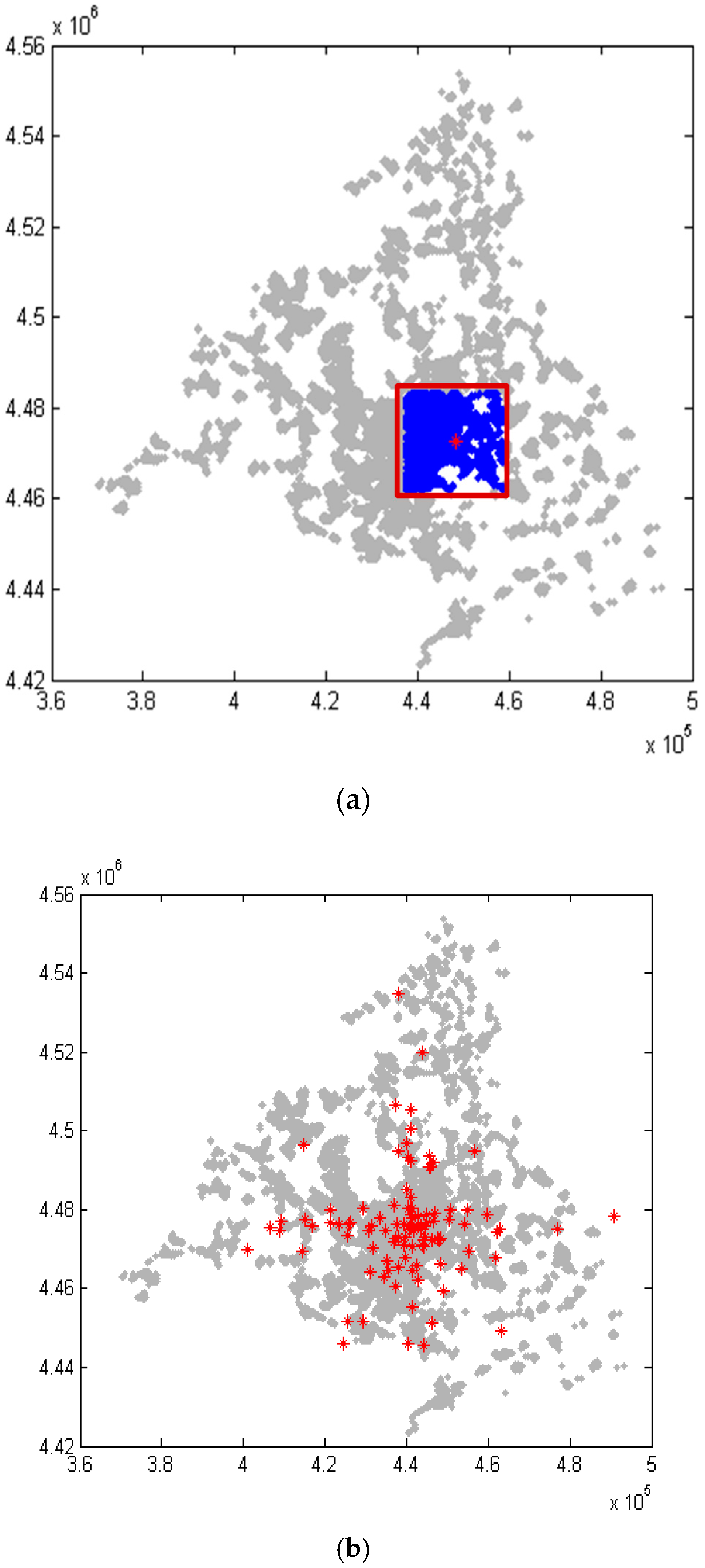Figure 1a shows the selection of elements in blue color for a sample with size L centered in a red point, while Figure 1b represents all central points (100 in total) analyzed for the validation process.

Model performance is linked to the regression between the number of failures predicted by the model in each sample and the number of failures actually observed. Two parameters were selected: the slope of the regression equation conditioned to null intercept and the regression coefficient R². Optimal value for both of them is one.

Sensitivity studies were carried out for checking validation procedure. Their aim was to quantify the uncertainty of the results of the validation (regression slope and regression coefficient) as a function of the parameters of the validation process. The analysis was focused on: size of the sample (in terms of number of zones), size of the zones of the sample and validation period.

The study of the size of the sample was done considering the obtained value for the quality indicators depending on the number of elements of the sample. The analysis was done for sample sizes between 100 and 500 elements. The analysis of the influence of the size of the zones was done modifying the dimension limits (L_min and L_max) keeping a constant minimum number of elements N_e. For the evaluation of the validation period, the period of available data was split into four years. Data from one year were used to adjust the model, which was then validated in the other three one-year periods. To do so, every possible combination was used for a total of 12 combinations.

The sensitivity study revealed that the number and size of the zones are relevant, but the parameter that most affects the results is the validation period. Because the result varies from one adjusting period to another, in order to identify the best model to represent the behavior, several periods have been used in each case and the best approach has been selected.

Based on such analysis, the proposed validation methodology considers a sample size of 500 elements of dimensions within 10 and 100 km. The performance of the models is studied in a wide range of zones from the smallest to the biggest ones that almost cover the entire system. The models were adjusted to the four available years (2011, 2012, 2013 and 2014) and each one of those was validated in the other three years. That way, 12 quality parameters were obtained for each of the selected variable combinations. Obtained results were compared to the order cero quality parameters.

The best variable combination is considered to be the one with a better global performance for the 12 cases analyzed. Global performance is based on a quality parameter defined as the distance to the optimum point in a plane defined by the two basic quality parameters: slope and correlation coefficient. Such distance (see Equation (5)) is the distance between the validation result and the optimum (adjusted slope equal to 1 and correlation coefficient equal to 1).

$$d=\sqrt{{\left(m-1\right)}^2+{\left(r-1\right)}^2}$$

(5)

where d is the distance, m is the slope of the regression line and r is the correlation coefficient.

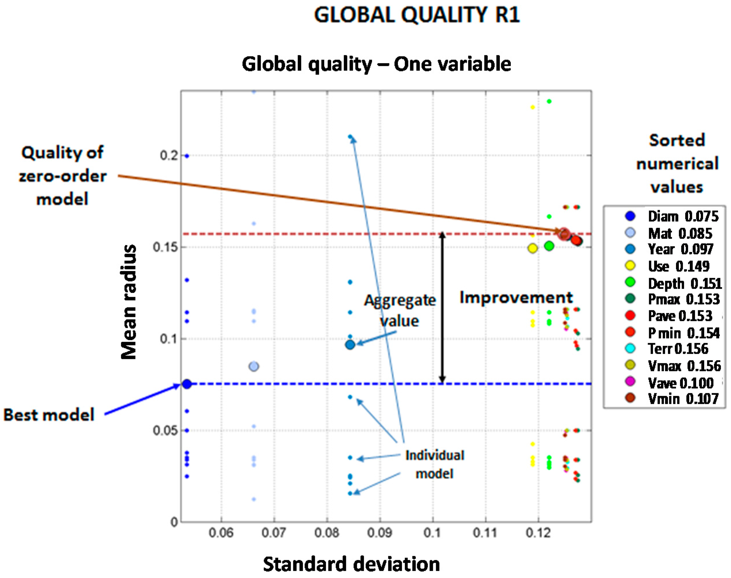
For each model built on a given variable combination, 12 sets of quality parameters are calculated (m, r, d). The selection is made considering the mean and standard deviation of the quality radius (see Equations (6) and (7)):

$$M=\frac{{{\displaystyle \sum }}_{i=1}^{12}{d}_i}{12},$$

(6)

$$SD=\sqrt{\frac{1}{12}{\displaystyle \sum }_{i=1}^{12}{\left(d_i-M\right)}^2}$$

(7)

Figure 2 illustrates how model results are compared and evaluated for a certain model, corresponding to a given combination of variables. The values of the mean and standard deviations of the quality radiuses are represented with a large dot. The individual values of the quality radiuses for each of the 12 validation cases are represented as smaller dots of the same color in the location corresponding to the standard deviation. The best model is the one closer to the origin of coordinates. For comparison purposes, the zero-order model is represented in brown color and highlighted with a horizontal line. The best model is also highlighted with a horizontal line. The distance between the best model and the zero-order model lines shows the improvement that can be achieved in the prediction by using the set of models under analysis.

3. Results

Following the procedure described in the previous section, firstly zero-order model results are presented. Later, results for both distribution lines and trunk mains are included for models ranging from order one to order five. With this approach, the influence of incorporating additional variables to the analysis can be analyzed with the aim of improving the models performance, firstly for distribution lines and later for trunk mains.

3.1. Zero Order Models

Zero order models do not consider any predicting variable in their formulation. Results obtained for both networks can be seen in

Table 3. Performance metrics for zero order models.

Category	Mean Slope (m)	Mean R2 (r)	Mean Radius (M)	Standard Dev. Radius (SD)
Distribution lines	1.107	0.975	0.157	0.125
Trunk mains	0.991	0.981	0.110	0.078

. Such analysis is based on the 12 validation cases described before. Model performance metrics are worse for the distribution lines than for the trunk mains although distribution network is larger. These performance values are used as the reference for the analysis of the multiple-variable models with the aim of quantifying the improvement of predictions’ performance as new explanatory variables are added.

3.2. First Order Models

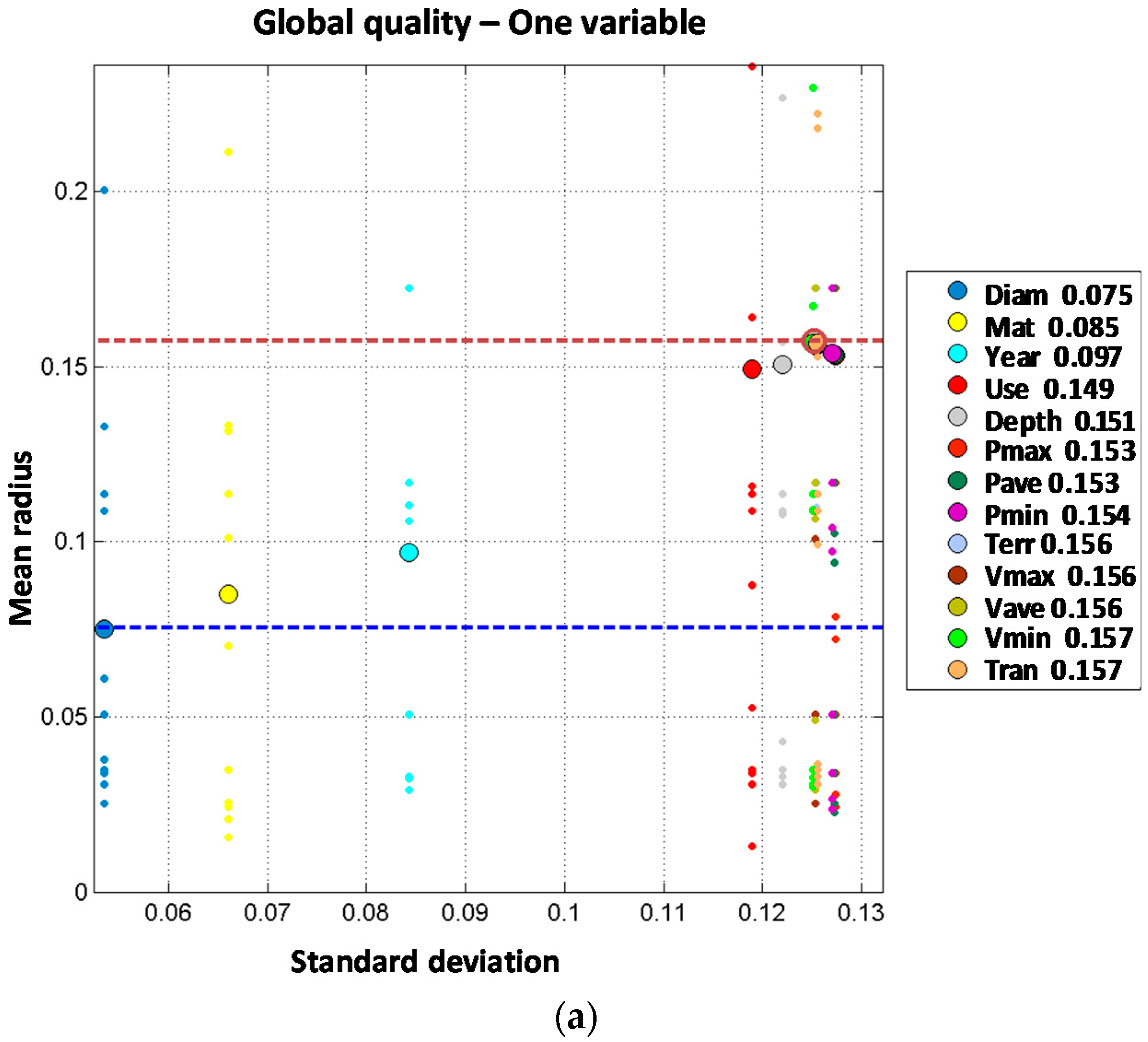
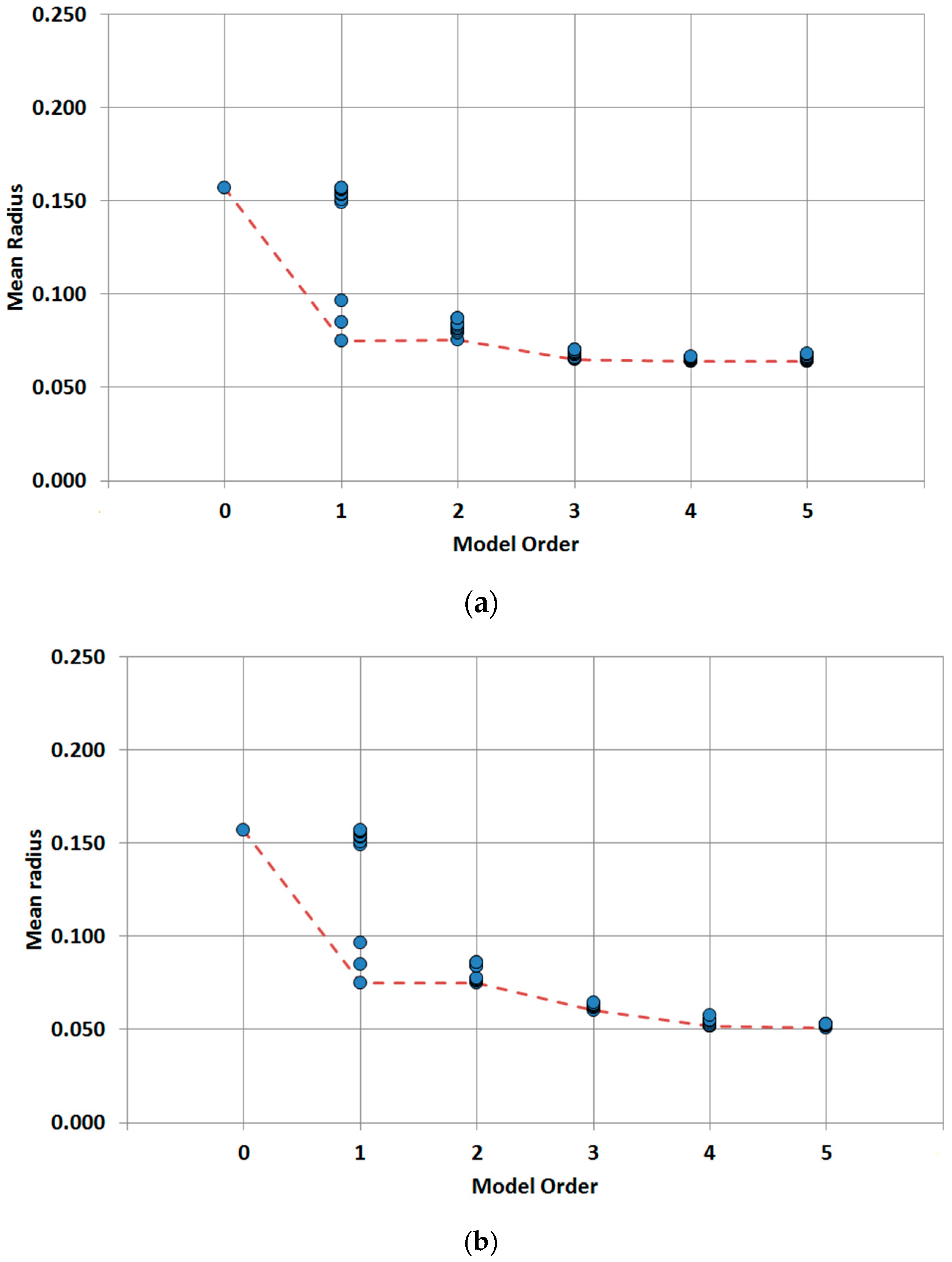
First order models are built with one single explanatory variable. Results obtained for distribution lines and trunk mains are shown on

Table 4. One variable models: predictive capacity for distribution lines (left) and trunk mains (right) networks.

	Distribution Lines				Trunk Mains
Variable	Mean Slope	Mean R2	Mean Radius	Std. Dev.	Mean Slope	Mean R2	Mean Radius	Std. Dev.
Diameter	1.021	0.971	0.075	0.053	0.948	0.977	0.073	0.063
Material	1.030	0.980	0.085	0.066	1.000	0.980	0.073	0.056
Year	1.049	0.980	0.097	0.084	0.971	0.979	0.086	0.059
Land Use	1.099	0.975	0.149	0.119	1.015	0.980	0.093	0.078
Depth	1.100	0.976	0.151	0.122	0.988	0.981	0.095	0.068
Pmax	1.112	0.975	0.153	0.127	1.010	0.981	0.096	0.078
Pave	1.112	0.975	0.153	0.127	1.006	0.981	0.098	0.078
Pmin	1.111	0.975	0.154	0.127	1.003	0.981	0.100	0.078
Terrain	1.108	0.975	0.156	0.125
Vmax	1.108	0.975	0.156	0.125	0.987	0.980	0.102	0.073
Vave	1.108	0.975	0.156	0.125	0.983	0.981	0.100	0.078
Vmin	1.107	0.975	0.157	0.125	0.995	0.981	0.107	0.078
Tran	1.108	0.975	0.157	0.126	0.993	0.980	0.103	0.074

and Figure 3.

Table 4 presents the performance results of the best model for each variable from all the aggregations considered. There are three variables that clearly provide a better prediction in both networks: diameter, material and year of installation. All other variables, including the hydraulic ones, provide a worse prediction with performance statistics closer to the zero order models.

Obtained results for trunk mains might be affected by the smaller number of registered breaks in comparison with the distribution lines. This might explain that for trunk mains the performance is not clearly improved beyond three variables, as will be seen later.

3.3. Distribution Lines

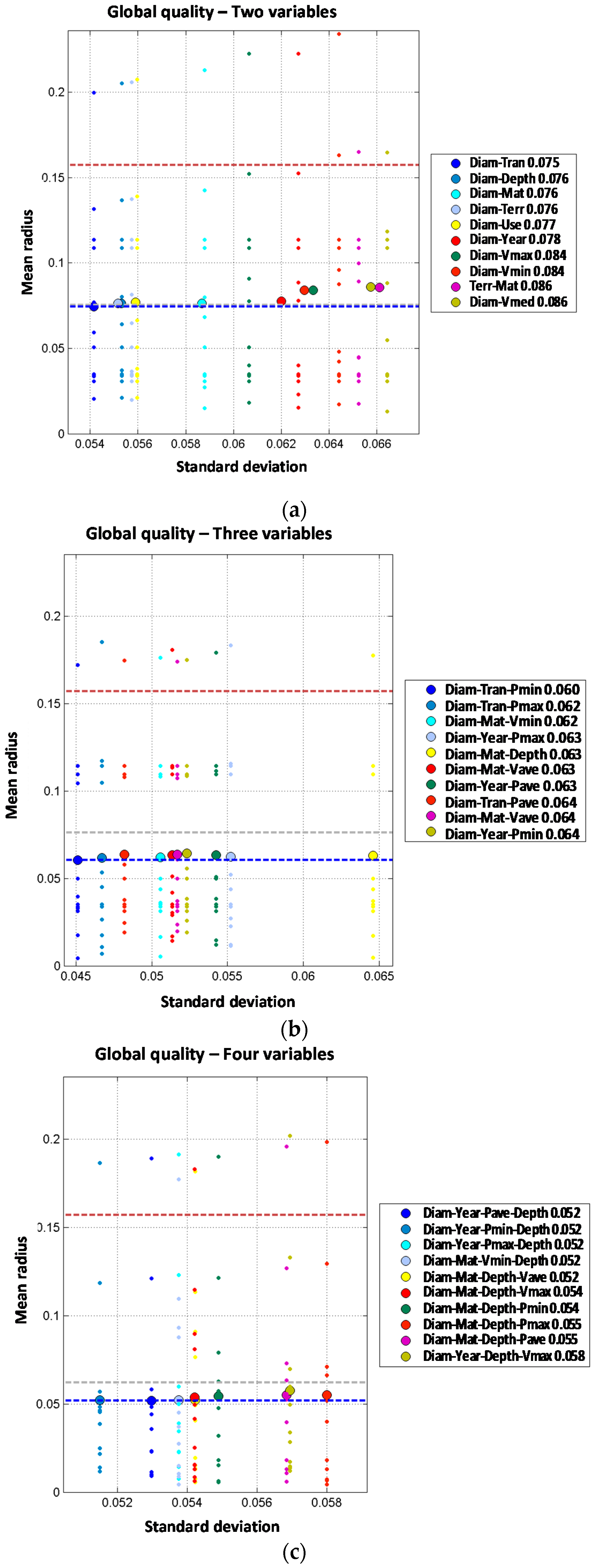
Based on previous results, multiple variable models were tested with the aim of improving the performance of single variable models. Two approaches are followed, considering independent variables or considering two joint variables plus additional independent variables. Firstly, the results of the independent variable models are explained and summarized in Figure 4.

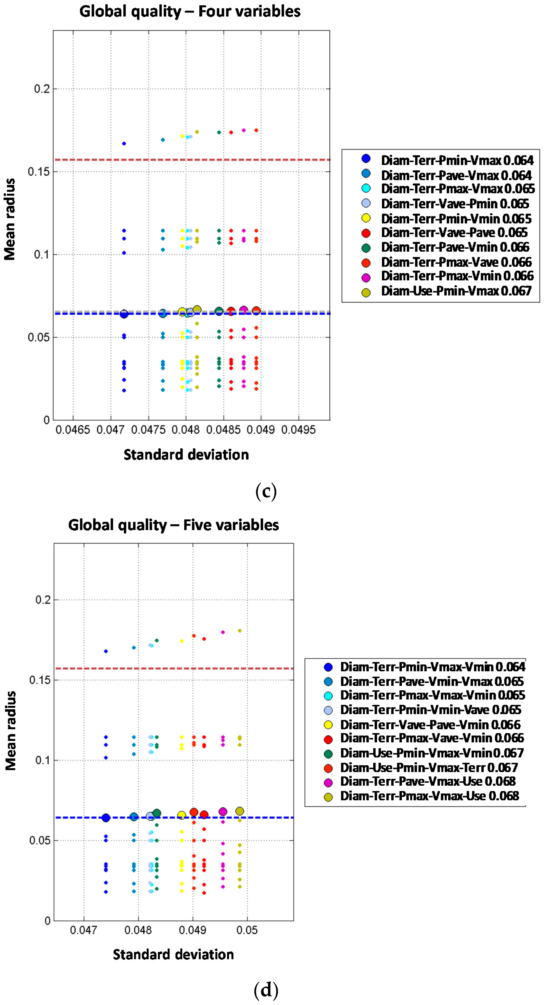
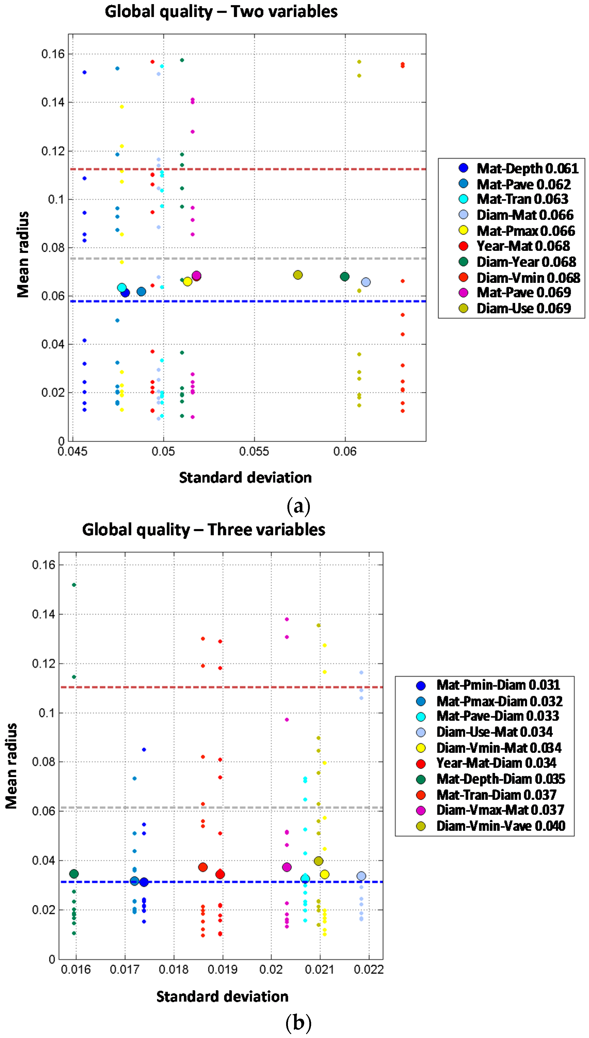
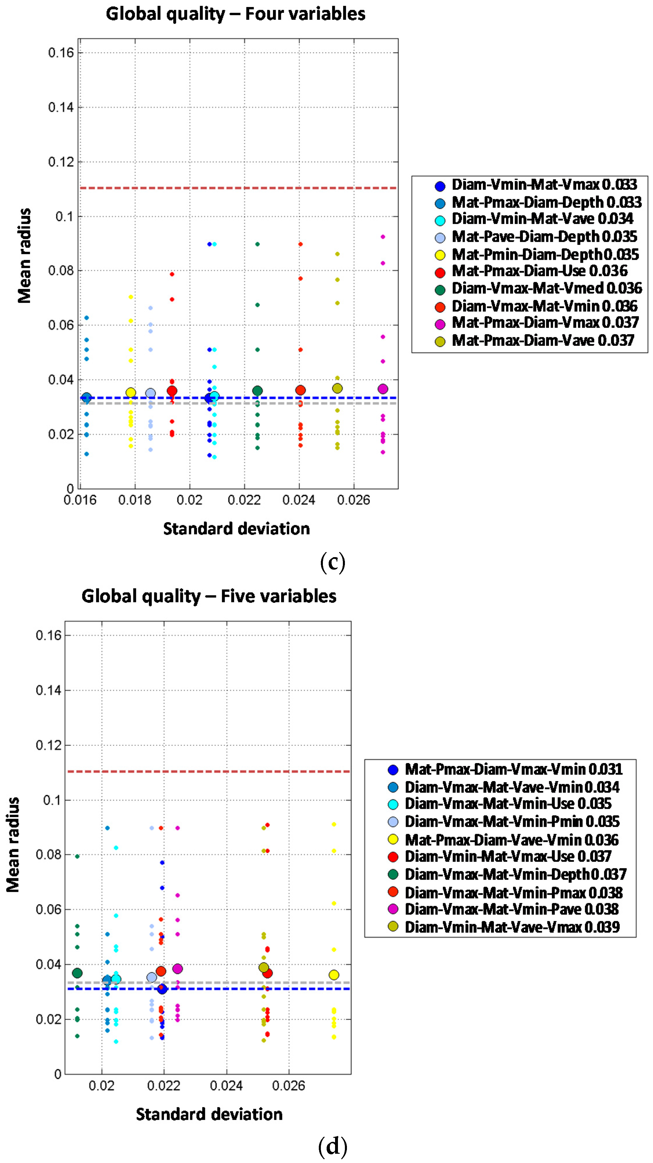
Two independent variable models are built based on the results of the single variable models. Thus combinations between diameter, material and year of installation are expected to produce a better prediction. Although the order two models generally improve the performance of single variable ones, none of them improve the prediction of the diameter order one model. Three independent variable models improve the order one and order two models. Again, diameter is involved in the best models. For the four independent variable models, the obtained results are quite similar to the three variable models. Diameter, type of terrain, minimum pressure and maximum velocity provide the best results. Thus, the mean radius obtained (0.064) slightly improves the order three result (0.065). The models built with five independent variables do not improve the results of the four independent variable models providing the same mean radius (0.064) in the best model. Thus, from the observed results, there is no advantage to introducing five variables in the predictive model.

Joint variable models are studied from the base of two joint variables incorporating, one, two or three additional independent variables to the model. Results are shown in Figure 5.

When analyzing the two joint variables models, the best combination obtained is diameter and transients index, with a mean radius of 0.075. Such result improves most of the single variable models but provides the same performance as the best one-order model (mean radius of 0.075 for the variable diameter). Other models combining material and type of terrain, depth or land use provide worse results than the single variable model. In any case, the improvement for single variable model to the two joint variables is far smaller than from the zero order model to the single variable models.

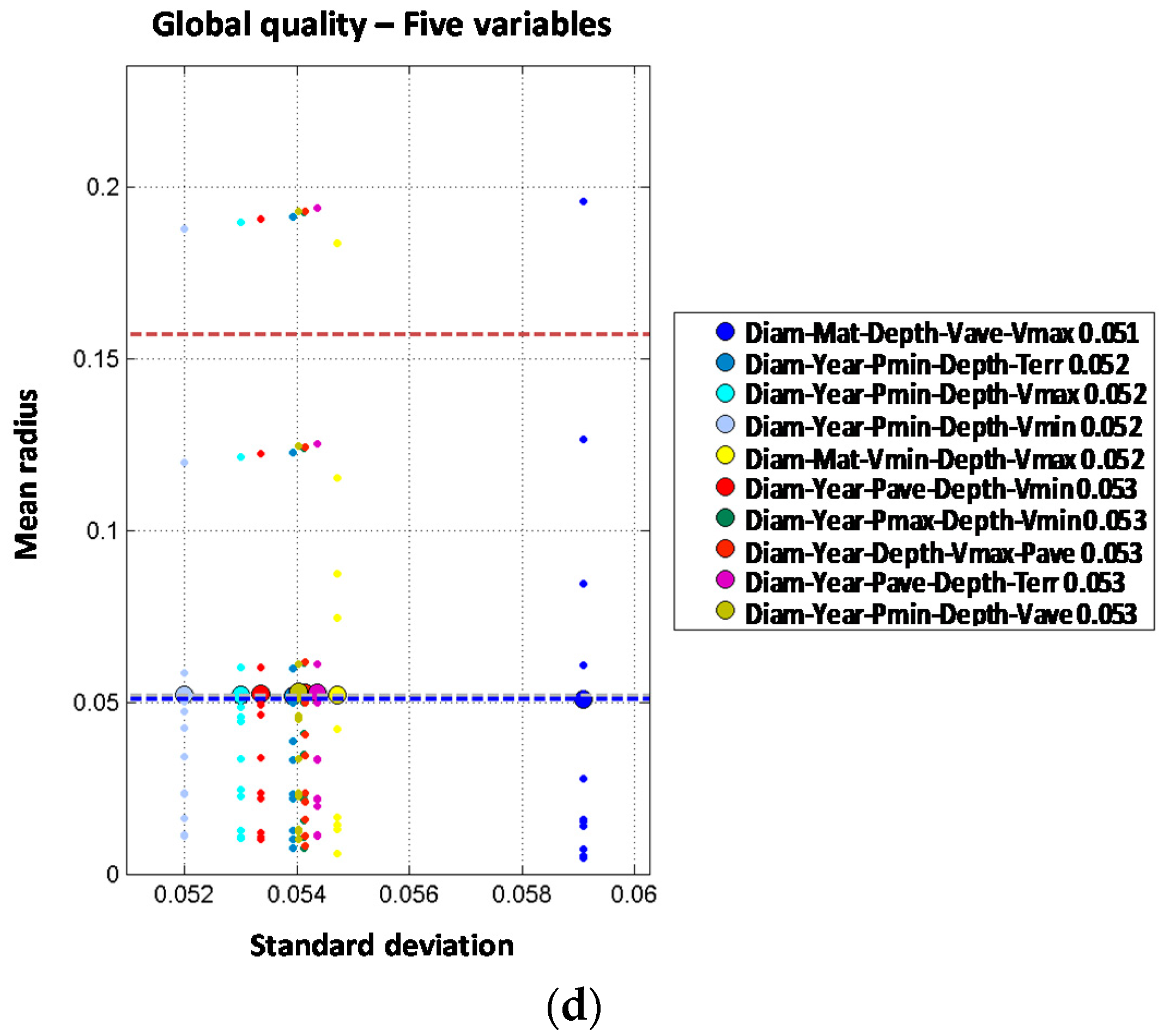
The 2J + 1I models are produced starting from the best two joint variable models adding an additional one (assumed independent from the others). From that point, several combinations provide a clear improvement in the performance of the prediction compared to those obtained with order one or two models. The combination of diameter plus transient index and minimum pressure clearly improves the results with mean radius decreasing from 0.075 to 0.060. It can be concluded that when comparing both types of order three models, the most accurate prediction is obtained with the 2J + 1I models. For the 2J + 2I models, the best results are obtained with the diameter-year variables combined with the depth and pressure variables (minimum, average or maximum). Diameter and material combined with minimum velocity and depth also provide good results. Best model provides a mean radius of 0.052 which reduces the values for the three variable models whose results are between 0.060 and 0.064. Thus, if the four variables are properly selected and combined, the performance of the prediction can be improved. The 2J + 3I models are built based on the results of the 2J + 2I models where a fifth independent variable is included. In this case, there is only one model that improves the performance of the four variable models. The combination of diameter and material with depth, average velocity and maximum velocity provides a mean radius slightly better (0.051 vs. 0.052).

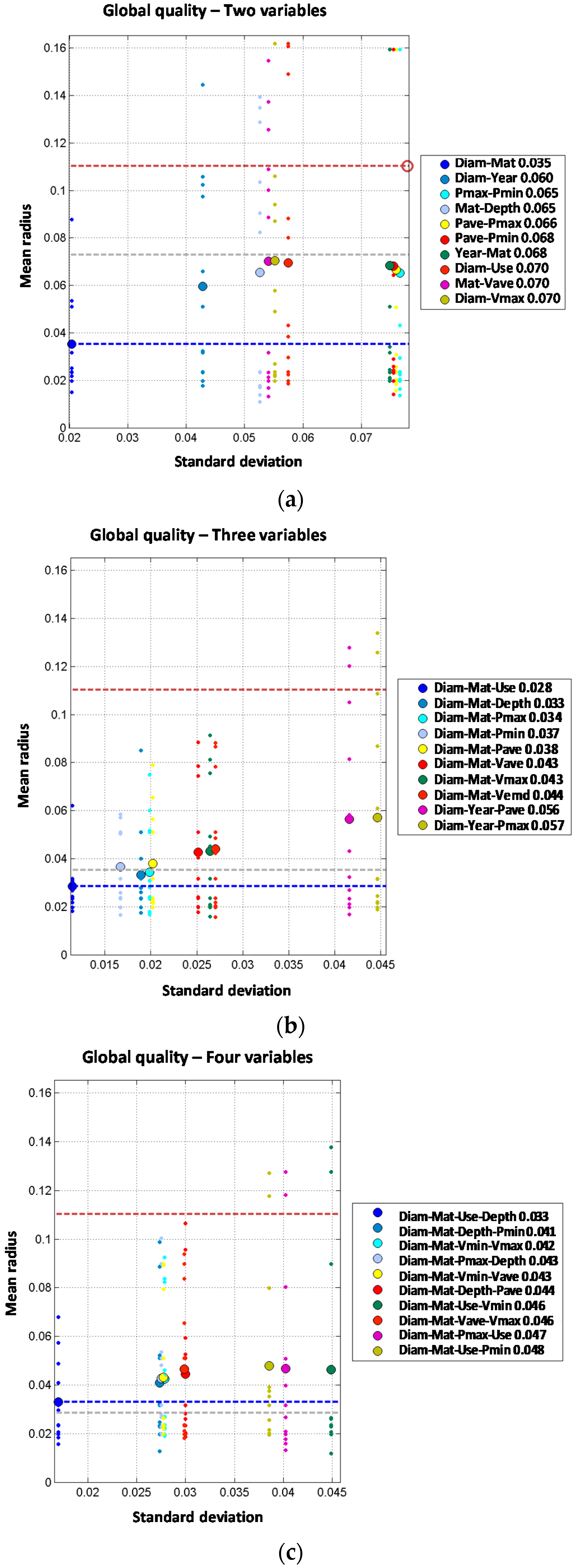
3.4. Trunk Mains

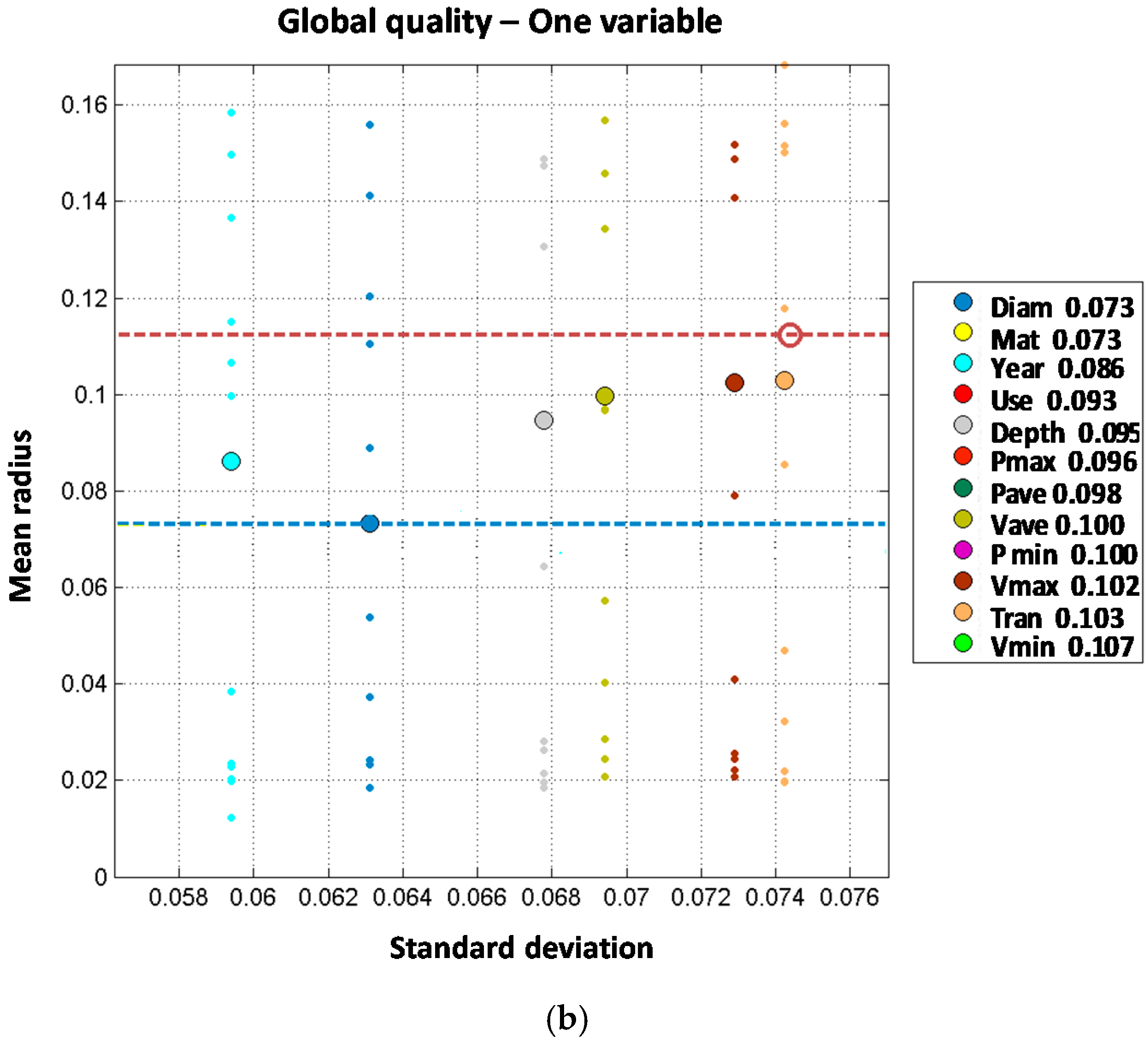
Like in the case of distribution lines models, trunk mains model results are analyzed in two steps. Independent variable models results are shown first in Figure 6, and later on two joint variable models plus additional independent variables are studied as shown in Figure 7.

When analyzing the two-order model for diameter and material combined, the result is significantly improved from a mean radius of 0.073 (for one variable model) to 0.035 when both variables are combined. Other independent combinations including diameter and other variables show less performance improvement, such as diameter with year (mean radius of 0.060), land use (0.070), or maximum velocity (0.070). Order two models including pressure variables also provide a significant improvement from first order models. Mean radius values for first order models including pressure variables range from 0.096 to 0.100. These values are reduced to 0.065 to 0.068 when two pressure variables are combined for maximum and minimum pressure (0.065), average and maximum pressure (0.066) and average and minimum pressure (0.068), suggesting that pressure range is more relevant than absolute value as a cause for pipe breaks. From the observed results, it may be concluded that single variable models performance is improved by incorporating an additional independent variable; especially if diameter is considered. Pressure and velocity variables show a good performance in terms of accuracy as well.

When material and diameter are combined with other variables in order three models, the performance is further improved. These two variables combined with land use provide the best result, with mean radius of 0.028. Combination of these variables with depth or pressure also improve order two results, but to a less extent, with mean radius of 0.033 and 0.038. However, when four independent variables are considered the mean radius is not improved. The optimal combination is obtained with diameter, material, land use and depth, with mean radius of 0.033. This means that by introducing a fourth variable (depth) the performance is reduced from the order three model (mean radius of 0.028) to the order four model (mean radius of 0.033). If five independent variables are used in the predictive model, the results are generally worse than for order three or four models. In fact, the best prediction reports mean radius of 0.047 for the combination of diameter, material, average velocity, maximum velocity and minimum velocity. As explained above, more complex models (orders four and five) do not show any clear improvement in the prediction of breaks on trunk mains. This might be explained because of the reduced amount of available data in trunk mains in comparison with the distribution lines, which limits our ability to estimate the probability distributions conditional to breaks.

Order two models have been analyzed combining every pair of variables. Two joint variable models report a significant improvement of the prediction performance. Models including material as one the predictive variables report the following values for mean radius: 0.061 for material combined with depth, 0.062 for material combined with average pressure and 0.066 for material combined with diameter or maximum pressure. These results clearly improve the best value of mean radius obtained with one predictive variable (0.073 for material). Similar results are obtained for combinations including diameter, reducing the mean radius from 0.073 to 0.066 (diameter combined with material). Other joint combinations of diameter with variables such as year, land use and velocity also improve the performance; on the other hand, combination of diameter with pressure or depth does not improve the results. Analyzing year, the third variable from one variable models list, the results are also improved from a mean radius of 0.086 for year alone to a mean radius of 0.068 for year jointly combined with material. Other joint combinations of year with other variables introduce slight improvements but not so relevant. Overall, models of two joint variables clearly improve the predictive performance as compared to single variable models. The best models are formed with the joint combination of material plus another variable such as depth, average pressure or transient index. In any case, the best result for two independent variables is clearly better than the best result for two joint variables (a mean radius of 0.035 for two independent variables versus a mean radius of 0.061 for two joint variables). For trunk mains, two independent variables models clearly show a better behavior than the two joint variables ones. This may be due to the limited availability of pipe break data in trunk mains.

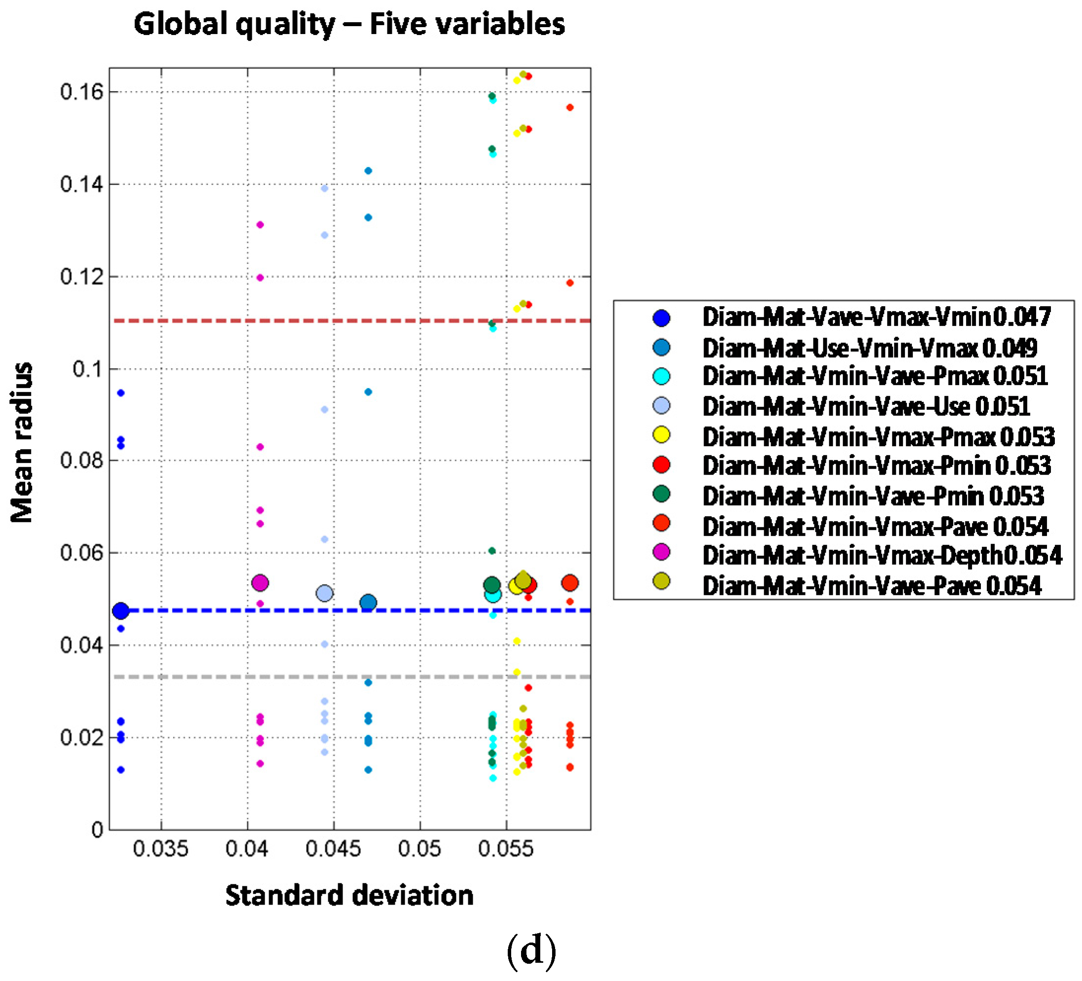
Models with two joint variables plus one independent variable are studied starting from the results of the order two models. Observed results show a very significant performance improvement, because most of the models report mean radius below 0.040 while the best mean radius for order two models (2J) was 0.061. Again, material is involved in the best models; in this case, jointly combined with any of the pressure variables and incorporating diameter as additional independent variable. The best results are obtained for minimum pressure (mean radius of 0.031), maximum pressure (mean radius of 0.032) and average pressure (mean radius of 0.033). Other combinations clearly improve the performance of order two models such as the joint combination of material and depth which is significantly improved from a mean radius of 0.061 (2J) to a mean radius of 0.035 by incorporating diameter as a third independent variable. Order four models formed by two joint plus two independent variables do not show any clear improvement in the prediction accuracy when compared with 2J + 1I. Best results are obtained for the joint combination of diameter and minimum velocity plus material and maximum velocity as well as the combination of material and maximum pressure plus diameter and depth. Such models report mean radius of 0.033 while for the corresponding order three models the mean radius obtained was 0.031. There is only one model from the set of two joint plus three independent variables models (order five) that increases the performance of order four models reducing the mean radius from 0.033 to 0.031. Such reduction is obtained with the joint combination of material and maximum pressure plus diameter, maximum velocity and minimum velocity. It must be highlighted that order three results are improved neither with order five nor with order four models despite the introduction of additional variables. This again might be due to the difficulty in estimating the probability distribution conditioned to breaks in trunk mains due to the limited number of pipe breaks registered. It is also noted that the year of installation is not present in the best models of order higher than three, while hydraulic parameters (pressure and velocity) are always present.

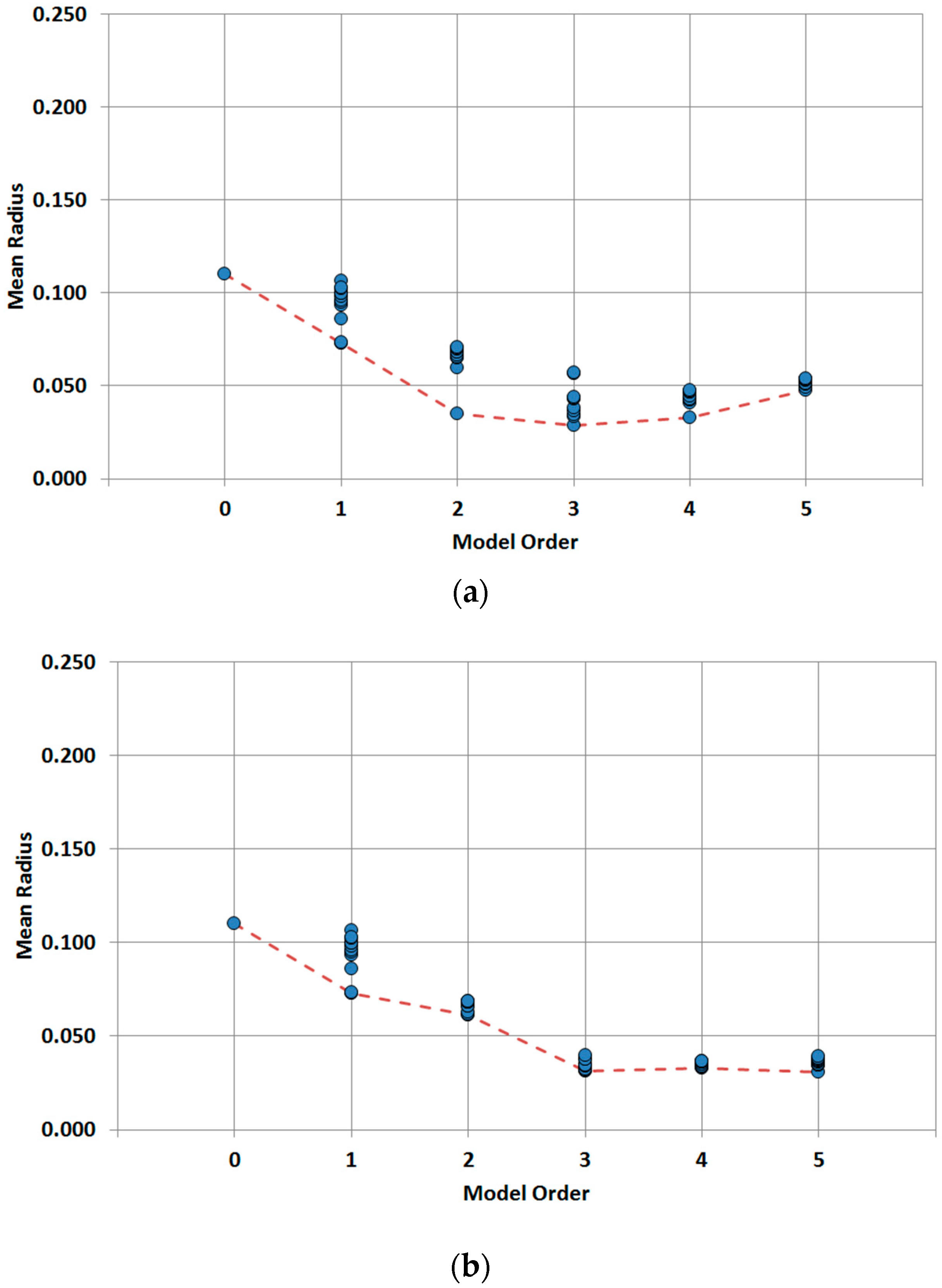
4. Discussion

Several models have been analyzed to predict the behavior of the distribution lines as well as trunk mains. The results obtained are compared with the aim of achieving the best prediction with the minimum number of variables. Such comparison is shown in Figure 8 and

Table 5. Best predictive models: Distribution lines. Values in parenthesis represent the number of intervals considered in variable discretization (F stands for full resolution).

Category	Ord.	Joint Variables	Independent Variables	Mean Radius
Independent Variables	2	-	Diam (8)–Terr (4)	0.076
	3	-	Diam (8)–Terr (4)–Pmin (F)	0.065
	4	-	Diam (8)–Terr (4)–Pmin (F)–Vmax (6)	0.064
	5	-	Diam (8)–Terr (4)–Pmin (F)–Vmax (6)–Vmin (6)	0.064
Joint Variables	2	Diam (6)–Tran (8)	-	0.075
	3	Diam (2)–Tran (7)	Pmin (F)	0.060
	4	Diam (8)–Year (4)	Pave (F)–Depth (3)	0.052
	5	Diam (2)–Mat (7)	Depth (5)–Vave (9)–Vmax (9)	0.051

for the distribution lines and in Figure 9 and

Table 6. Best predictive models: Trunk mains. Values in parenthesis represent the number of intervals considered in variable discretization (F stands for full resolution).

Category	Or.	Joint Varables	Independent Variables	Mean Radius
Independent Variables	2	-	Diam (10)–Mat(3)	0.035
	3	-	Diam (10)–Mat (3)–Use (6)	0.028
	4	-	Diam (10)–Mat (3)–Use (6)–Depth (F)	0.033
	5	-	Diam (10)–Mat (3)–Vave (F)–Vmax (2)–Vmin (2)	0.047
Joint Variables	2	Mat (11)–Depth (10)	-	0.061
	3	Mat (11)–Pmin (F)	Diam (3)	0.031
	4	Diam (F)–Vmin (F)	Mat (2)–Vmax (9)	0.033
	5	Mat (11)–Pmax (6)	Diam (3)–Vmax (3)–Vmin (3)	0.031

for the trunk mains. The different order models are shown versus the obtained mean radius so that the best performances of each model order are clearly compared.

Regarding the distribution lines, there are multiple variables involved in the best models. For models of order higher than two, there are many variable combinations that produce similar results because the differences between the ten best models selected are very small. The small differences in performance between sets of variables do not seem to be very relevant, given the variability of results obtained in the 12 validation cases considered. The only common variable that appears in all best combinations is the pipe diameter which results to be a critical parameter in the predictive models. For independent variable models the best prediction is obtained by adding an additional variable to the best model of the previous order. In this case, best models are obtained by combining diameter and terrain with hydraulic variables (pressure and velocity). Rather surprisingly, year of installation does not appear in the best model of each order. In the case of two joint variables, the combinations of diameter and year or diameter and material are present in most models analyzed and they clearly outperform the independent combination of diameter and terrain for orders higher than three. The joint combination of diameter and year seems to be more robust than diameter and material because it dominates the best models of order five.

The developed analysis suggests that the best predictive model is for the distribution lines the order four model with two joint variables and two additional independent variables, because adding a third independent variable makes the calculation more complex without a significant performance improvement, as can be seen in Figure 8 and Table 5. The best variable arrangement in this case is the joint combination of diameter and year plus average pressure and depth of installation, although the other pressure variables also provide similarly good results.

The analysis of the results of trunk mains reveals a wider dispersion between performances of models built with different sets of variables than in the case of the distribution lines. As can be seen in Figure 9 as well as Table 6, higher order models do not improve the performance, thus the optimum model is the order three model formed by three independent variables. Again, the diameter is a critical parameter to predict the behavior of the assets, but material is also a relevant parameter to be considered. As in the case of the distribution lines, for independent variable models the best models are obtained by adding an additional variable to the best model of the previous order, up to order five, where performance clearly degrades with respect to the previous order. When considering the joint variable models there are no combinations of joint variables that can be identified as dominant over the others among the best models. Diameter and material appear in most cases combined with hydraulic variables, but there are many possibilities. In any case, the joint variable models are always inferior to the independent variable models.

Based on obtained results the proposed predictive model for trunk mains is the three independent variable model formed by diameter, material and land use.

Comparing the obtained results for each type of network, it can be inferred that pipe diameter emerges as a critical variable to explain the behavior of any of the networks. There is a significant difference in the performance of the results obtained for each type of network: for the distribution lines the joint models show better performance, while for trunk mains the best performance is obtained with independent model. Such difference might be affected by the different amount of analyzed data in each case. The fact that there is much more information for the distribution lines from the recorded breaks can explain such difference in the performance as well as the fact that increasing the number of variables (independent variables) in the trunk main models does not improve the performance. Results for trunk mains show that the performance tends to decrease from a maximum obtained for the third order models to higher order models. The number of observed breaks per year in the distribution lines is about 2000, while in the trunk mains is always smaller than 100. This means that the estimation of the probability distribution of any variable conditioned to breaks is much more robust in the case of the distribution lines than in the case of trunk mains, especially if the number of intervals considered in the analysis is large. For practical purposes the estimation of the joint probability distribution of two variables conditioned to breaks in trunk mains is limited to cases where only two or three intervals are considered in each variable and this fact clearly limits the predictive skill of such models.

The results shown are highly influenced by the specific characteristic of the network where the methodology is applied (Canal de Isabel II network). However, the procedure allows determining the number of variables to be used in a predictive model and the identification of such variables. Slight variations are expected depending on specific networks where the proposed methodology might be applied. The results show that performance is rapidly improved by introducing two or three variables. Anyway, it is quite clear that incorporating variables beyond a certain level in the analysis do not add performance in the prediction.

5. Conclusions

The research compiles and analyzes a large set of collected data on pipe breaks. With the proposed methodology, the influence of different variables on failure rates can be quantified. Multiple models are studied combining several explanatory variables with the aim of proposing an accurate break model for distribution lines and trunk mains.

The statistical dependence of pipe breaks on each explanatory variable depends on the type of network. Multiple variables have been studied to provide an accurate failure prediction based on network parameters rather than in simple statistical data, which is only based on recorded performance of the network.

From all the variable combinations (joint and independent models), the best prediction for the distribution lines is obtained with the model formed by diameter and year as joint variables plus average pressure and depth as independent variables. Such model provides a mean radius of 0.052, which is a significant improvement over the values obtained for the zero order model (0.157) or for the material single variable model (0.075). The results of trunk mains are conditioned by the fact that the number of registered breaks is clearly smaller in comparison with the distribution lines. For this case, results show that prediction is not increased in higher order model. This is explained because it is difficult to build a complex model form such a small number of breaks. Based on that, the best prediction is obtained for the three independent variable model formed by diameter, material and land use. Obtained mean radius is 0.028, which improves significantly the zero order model performance, 0.110, or the first order model performance, 0.073, obtained with material.

The discussed models enable to predict the pipe breaks so that this information can be used to support economic analysis of repair versus replace strategies. This information helps water companies to plan their maintenance and renewal strategies. This all results in a better management of the water distribution asset and a better level of provided service by the supplier.

The observed relation between the performance of the predictive model and the number of considered variables obtained in the study shows that there are no clear advantages in considering a large set of predictive variables. Using a reduced set of explanatory variables also increases the reliability of the proposed predictive models and makes the investment/replacement decision making much easier for water supply companies reducing the complexity of the lifetime estimation models.