Space–Time Characterization of Rainfall Field in Tuscany

1
LaMMA Consortium, Via Madonna del Piano 10, Sesto Fiorentino 50019, Italy
2
National Research Council, Institute of Biometeorology, Via Gino Caproni 8, Florence 50141, Italy
Water 2017, 9(2), 86; https://doi.org/10.3390/w9020086
Submission received: 28 October 2016
/
Accepted: 23 January 2017
/
Published: 31 January 2017
(This article belongs to the Special Issue Advances in Hydro-Meteorological Monitoring)
Abstract
:Precipitation during the period 2001–2016 over the northern and central part of Tuscany was studied in order to characterize the rainfall regime. The dataset consisted of hourly cumulative rainfall series recorded by a network of 801 rain gauges. The territory was divided into 30 × 30 km2 square areas where the annual and seasonal Average Cumulative Rainfall (ACR) and its uncertainty were estimated using the Non-Parametric Ordinary Block Kriging (NPOBK) technique. The choice of area size was a compromise that allows a satisfactory spatial resolution and an acceptable uncertainty of ACR estimates. The daily ACR was estimated using a less computationally expensive technique, averaging the cumulative rainfall measurements in the area. The trend analysis of annual and seasonal ACR time series was performed by means of the Mann–Kendall test. Four climatic zones were identified: the north-western was the rainiest, followed by the north-eastern, north-central and south-central. An overall increase in precipitation was identified, more intense in the north-west, and determined mostly by the increase in winter precipitation. On the entire territory, the number of rainy days, mean precipitation intensity and sum of daily ACR in four intensity groups were evaluated at annual and seasonal scale. The main result was a magnitude of the ACR trend evaluated as 35 mm/year, due mainly to an increase in light and extreme precipitations. This result is in contrast with the decreasing rainfall detected in the past decades.
1. Introduction
In recent decades, there has been a gradual increase in the average temperature of the atmosphere. Global warming has determined a higher water vapor concentration and thus an increase in global precipitation [1]. Despite this overall scenario, a decrease in rainfall was found in the Mediterranean area; for example, experimental results for Italy and Spain indicated a reduction in precipitation [2,3]. Along with the decrease in the average rainfall amount, there has been a change in rainfall patterns, with extreme events becoming more frequent [4]; in particular, Brunetti [5] and Martinez [6] found similar results for Italy and northern Spain (Catalonia). The pattern was not homogeneous on the Italian territory, being more pronounced in the north [7].
Climate change may cause increased drought and extreme events, therefore the study of the evolution of the rainfall regime is a very important task in order to construct a hydrological model, prevent flooding and hydraulic risk [8,9]. It is thus necessary to study rainfall phenomena in different time periods. Evaluation of the rainfall regime for relatively long time periods, annual or seasonal, is essential for the study of climate change and hydrological models. Prevention of hydraulic risks requires an assessment of rainfall phenomena for relatively short time periods, daily or hourly. In this perspective, the amount of rain falling on the territory has to be estimated and its uncertainty evaluated in order to establish the reliability of the results.
In this study, the rainfall regime in the Tuscany region was analyzed during the years 2001–2016. A rain gauge network was used that provides measurements of the cumulative rainfall relative to a small area (in the order of hundreds of square centimeters). There were only a limited number of rain gauges in the territory, the typical distance between them was a few km in more populated areas and more than ten km in hilly areas.
The spatial variability of the cumulative rainfall field implies that for a distance of a few km, the values of the correlation coefficient of such an observable is very low [10,11,12]. Therefore, by means of a rain gauge network with such a low density, it was not possible to reconstruct the details of the rainfall field using some spatialization techniques. Given the limitation of the instrumentation, an observable was chosen that evaluates the overall rainfall amount on a selected area: the Average Cumulative Rainfall (ACR) i.e., the cumulative rainfall averaged over the area. The spatialization technique chosen to estimate the ACR was Non-Parametric Ordinary Block Kriging (NPOBK) [13,14,15,16,17,18]. It allows the best value to be estimated and the standard deviation of the ACR, which is a measure of the uncertainty.
An observable closely related to the ACR is the Rain Volume (RV) i.e., the ACR multiplied by the area; RV can be estimated during thunderstorms by means of the area time integral method, a technique based on non-quantitative rainfall detection [19,20]. Griffith et al. [21] used geosynchronous visible or infrared satellite imagery to estimate rainfall over large space and time scales. All these techniques are characterized by lower spatial and temporal resolution.
The estimation of ACR degrades the spatial resolution compared to rain gauge measurements but it allows the amount of rainfall to be assessed on a selected area. In this context, the Tuscany territory was divided into square areas where the ACR was estimated. The uncertainty of the ACR decreases by increasing the area under consideration, but the increase in the area deteriorates the spatial resolution. A compromise was therefore found for the area size that allows a satisfactory spatial resolution and an acceptable uncertainty of ACR estimates.
The annual, seasonal and daily ACR were estimated for all the areas, highlighting the difference in the precipitation amount in different parts of the territory. The trend detection of annual and seasonal ACR time series was performed by means of the Mann–Kendall test. The analysis showed higher rainfall in the north-western area, and an overall increase during the period, more pronounced on the Tyrrhenian coast. This increase occurred mainly in winter. The precipitation increase in Tuscany is contrary to that of previous decades, when a null or negative trend was recorded [22,23]. The analysis of daily ACR time series showed an increase in extreme events, therefore in this case, in agreement with the results obtained for the previous years [5,7].
2. Data and Methodology
2.1. Data
The instrumentation used to evaluate the rainfall field was a network of weather stations equipped with rain gauges and other meteorological sensors. The rain gauges measure cumulative rainfall with an hourly accumulation time. The network is managed by the Hydrological Service of Tuscany Region that provides the quality control of the data. The area covered extends over the Tuscany region and neighboring areas of Emilia-Romagna, Lazio and Umbria. Figure 1 reports the rain gauges located in Tuscany in March 2015.
The number of rain gauges increased during the period considered (2001–2016) as new gauges were installed: 325 in 2001 and 801 in 2016. The cumulative rainfall for different accumulation times was evaluated for each rain gauge by adding the hourly measurements. The accumulation times considered were annual (from 1 September to 31 August); seasonal (from 1 September to 30 November in autumn; from 1 December to 28 or 29 February in winter; from 1 March to 31 May in spring; and from 1 June to 31 August in summer); and daily.
Only cumulative rainfall measurements of rain gauges that had recorded more than 90 percent of the hourly measurements during the accumulation time were considered. The results obtained were multiplied by the ratio between the number of hours of the accumulation time and the number of hourly measurements recorded in order not to underestimate the result. This procedure eliminates the bias due to a loss of hourly measurements, but introduces an increase in the uncertainty of the cumulative rainfall.
2.2. The NPOBK Technique
The complete characterization of the rainfall regime on the territory can be obtained by evaluating the amount that falls on an arbitrary area for an arbitrary time period; this can be obtained by means of ACR, which can be expressed in terms of rain rate as:
where t is an arbitrary instant of time period T, x an arbitrary point inside area A, r the rain rate evaluated in point x and time t, C(x) the cumulative rainfall in point x.
Determination of the rain rate field for every instant and every point is a necessary and sufficient condition to determine the ACR for any space–time domain. This is obviously impossible given the limitations of the measurements provided by the available instrumentation; the rain gauges perform cumulative rainfall measurements that represent an integral of the rain rate, furthermore they are only installed at a limited number of points. The first limitation implies that 1 h is the shortest accumulation time to evaluate the ACR. The second implies that the ACR estimates should be made by means of a spatialization of the measurements. The spatialization technique used was the NPOBK method; it is based on the assumption that the cumulative rainfall field C(x) is statistically describable by means of a second-order stationary random function [13,14,15,16,17,18] i.e., the first and second moments are invariant under translations; they are described by means of the following equation:
where E[] is the mean value operator, m the mean value of cumulative rainfall independent of point x, F(h) the correlation function that depends only on the distance h of the two points as the isotropy of the field was also assumed [13]. In this perspective, ACR is described by means of a random variable (R_ACR), its mean was considered the best estimate of ACR and its variance a measure of uncertainty. The technique produces an interpolation function that gives the best unbiased linear estimate of the mean of R_ACR (Equation (3)) and its variance () (Equation (4)):
where C(xα) is the rain gauge measurement value on the points xα, A the area, T the accumulation time, γ(x, y) the variogram relative to the pair of points x and y. The parameters λα and μ are the solution of the following linear equations system:
The uncertainty of the ACR estimate was a decreasing function of the number of rain gauges installed within and near the analyzed area, so the size of the area had to be large enough to contain a sufficient number of these in order to perform acceptably accurate estimates. It is worth noting that to estimate ACR, only rain gauge measurements placed within or in proximity to area A were used. The use of measurements away from the area decreases the value of the variance very little at the expense of a substantial increase in the calculation time required.
The variogram, for the isotropy of the model, is a function that depends only on the distance of the points and it can be evaluated by the following equation:
C(x) is second-order stationary therefore the second term of the second member is equal to zero (Equation (2)). The sample values of the variogram were estimated nonparametrically, i.e., without supposing the shape a priori, evaluating approximately the second member of Equation (6) by means of the following:
where C(xi) is the cumulative rainfall measurement of the rain gauge installed in point xi. The sample values of the variogram were determined accurately by considering large values of n(h), therefore using the measurements of rain gauges installed in a large area N. To determine the largest area N where the field was stationary, the variogram was evaluated using measurements of the rain gauges located within increasingly larger areas centered on the same point. When increasing the size of the area, a significant increase was observed in the sill evaluation of the variogram, so the field cannot be considered stationary. Indeed, the apparent growth of the sill is due to the non-stationarity of the field, so in this case, the second term of the second member of Equation (6) is not negligible and therefore Equation (7) does not accurately determine the sample values of the variogram. In all the cases studied (Section 3.1), the largest area N where the cumulative rainfall field was stationary contains the area A where the ACR was estimated (a 30 × 30 km2 square area), therefore the cumulative rainfall is also stationary in area A and the NPOBK method can be applied to estimate the ACR in this area. To avoid negative values of the R_ACR variance, a conditionally negative defined variogram [15,16,17,18] was assumed. For this reason, the variogram was determined by fitting the sample values with the following exponential function [18]:
where Q and r are the fitting parameters.
The rain rate field was always different for each area and in each time as every rainfall event has its own peculiarities, so the characteristics of the accumulation rainfall field differed for each analyzed case. For this reason, for each ACR estimate, the procedure described above was repeated; first the maximum area was determined where the accumulation rainfall field was stationary, then the variogram was calculated using Equations (7) and (8).
2.3. ACR Estimation
The territory was divided into square areas, the annual, seasonal and daily ACR(Ai,Tj) were evaluated for each area during the period 1 March 2001–31 May 2016. Ai denotes an arbitrary area in Figure 2, Tj an arbitrary year, season or day. Each area was identified by means of its center, latitude and longitude, expressed in decimal degrees. The annual and seasonal ACR were estimated by means of the NPOBK technique described in Section 2.2. The relative error, defined by 3σACR/ACR, was evaluated. Only ACR estimates with relative error lower than 90 percent were considered sufficiently accurate.
The size of the areas had to be large enough to contain a sufficient number of rain gauges in order to perform an acceptably accurate ACR estimate. Conversely, the spatial resolution of the accumulation rainfall field is better for small areas. Based on these statements the choice of the size of square areas was 30 × 30 km2, which is the best compromise between a good resolution and an acceptable uncertainty of the ACR estimates. Only the northern and central part of Tuscany was examined, as the low density of rain gauges installed in the southern part of the region does not allow the ACR to be estimated with sufficient accuracy (Figure 2).
Over a hundred thousand daily ACR had to be estimated, which is an enormous number. The algorithm to perform the NPOBK is computationally expensive so it was not possible to estimate the daily ACR in a reasonable amount of time. For this reason, the NPOBK technique was not used and another computationally less expensive technique had to be considered. The daily ACR were therefore estimated averaging the cumulative rainfall measurements recorded by rain gauges within the study area. This technique, identified as AM, provides less accurate estimates than the NPOBK technique, and also does not allow the uncertainty to be evaluated.
To establish whether the estimates obtained by means of the AM technique were sufficiently accurate for the aims of this study, the daily ACR estimated by AM and NPOBK techniques was compared for some special cases. The discrepancy of the values in all cases was in the order of a few tens of percentage points, a quantity considered small enough.
2.4. Local Rainfall Regime
2.4.1. Time Average of Local Rainfall
For each area (Figure 2), in order to establish the difference of the typical rainfall amount falling in different zones of Tuscany, the means of the annual and seasonal ACR over the entire period (ACR_AV) were considered:
where Ai is an arbitrary area (Figure 2), T1,…. Tn, all the years or all autumn, winter, spring and summer seasons of the considered period, f the joint probability density function of the random variables R_ACR(Ai,T1), …, R_ACR(Ai,TN).
The exact value of ACR_AV could not be established as the joint probability density function was unknown. ACR_AV was therefore evaluated approximately averaging the values of the ACR estimated for each year or season:
2.4.2. Trend Analysis of Local Rainfall
To establish the rainfall regime evolution in each area, in particular if an increase or a decrease in ACR occurred, the trend analysis of annual and seasonal ACR(Ai,Tj) time series was conducted together with an evaluation of the magnitude of the trend.
The trend analysis of the time series was performed by means of the non-parametric Mann–Kendall test for autocorrelated data [24,25]. The Z statistic used to perform the trend analysis is a random variable whose probability density function is known and can be approximated to a Gaussian with zero mean and standard deviation equal to 1 for time series with a number of elements greater than or equal to 10. The significance level chosen to reject the null hypothesis, i.e., the absence of a trend, was 0.05, corresponding to Z > 1.96 (positive trend) or Z < −1.96 (negative trend).
2.5. Global Rainfall Regime
2.5.1. Global Rainfall
Annual, seasonal and daily ACR evaluated over the entire territory (ACR_TOT) was analyzed in order to study the overall evolution of the rainfall regime. The cumulative rainfall field was not second-order stationary as the area was too large, so the NPOBK technique was not applicable. It was therefore chosen to evaluate ACR_TOT by means of the mean of ACR in all areas (Figure 2) corresponding to the same accumulation time:
where Tj is an arbitrary year for annual ACR_TOT, or an arbitrary autumn, winter, spring, summer season for seasonal ACR_TOT, or an arbitrary day for daily ACR_TOT; A1…..Am are all the areas in Figure 2, f the joint probability density function of random variables R_ACR(A1,Tj), …, R_ACR(AM,Tj).
Once again, the joint probability density function of the R_ACR was unknown so the ACR_TOT was evaluated, approximately averaging the ACR estimates;
2.5.2. Observables for the Study of the Global Rainfall Regime
ACR_TOT.
Number of rainy days (NRD): the number of days during which daily ACR was greater than 1 mm. If the ACR was less than 1 mm, the day was considered not rainy.
Mean intensity of precipitation (MIP): the ACR_TOT divided by NRD.
The sum of daily ACR_TOT falling into these intensity groups: ACR_TOT <10 mm (SD0), 10 mm < ACR_TOT < 25 mm (SD10), 25 mm < ACR_TOT < 40 mm (SD25), 40 mm < ACR_TOT (SD40).
The time scale will be indicated in subscript to the name of the observable (ann, aut, win, spr, sum indicate the annual and seasonal time scales respectively).
It should be noted that the daily ACR evaluated over relatively large areas never presents the peak of daily cumulative rainfall values observed by some rain gauges, which take measurements on a much smaller area. The correlation coefficient of daily cumulative rainfall presents values significantly lower than 1, even for distances of a few km [10,11,12]. This implies that the peak values may not remain on the whole area. For this reason, the threshold value (40 mm) chosen for the last intensity group is significantly lower than the cumulative rainfall measurements of some rain gauges during an extreme event, which may exceed 100 mm.
The trend analysis was performed for all time series and the magnitude of the trends was computed.
3. Results
3.1. Evaluation of the Variogram
The sample values of variograms for all the years and seasons were derived by means of Equation (7), using the cumulative rainfall measurements inside 30 × 30, 40 × 40, 50 × 50, 60 × 60, 70 × 70 km2 square areas. The variograms were evaluated by fitting the sample values obtained by the measurements within the largest areas where the condition of stationarity occurred. In almost every case, the stationarity of the field is checked inside areas of 60 × 60 km2 or smaller. In all cases, the value of the SILL (Q parameter of Equation (8)) was between 40,000 and 600,000 mm2 for the annual ACR and between 3000 and 100,000 mm2 for the seasonal ACR. The r parameter (Equation (8)) was between 7000 and 30,000 m for the annual ACR and 15,000 and 70,000 for the seasonal ACR. As an example, Figure 3 reports the variograms of annual and seasonal ACR for the year 2009–2010 (areas centered at lat. 43.75°, lon. 11.25°). In all cases, the 60 × 60 km2 area was the largest where the stationarity condition was verified, except in spring 2010, where this condition was also verified for the 70 × 70 km2 area.
3.2. Estimation of Rainfall Amount
The annual and seasonal ACR were estimated for each area (Figure 2) by means of the NPOBK technique during the considered period. Examples are given in Table 1 (for some areas and all years and seasons) and in Figure 4 and Figure 5 (for all areas and some years and seasons). The typical values of the relative error were some tens of percentage points; in all cases, it was lower than 75 percent. The density of rain gauges was not homogeneous, it was greater near the main towns and in the most populated areas in general (Figure 1), therefore the relative error decreases accordingly. New rain gauges were installed during the considered period, so in some areas the uncertainty was lower when evaluated more recently. For some seasons and areas, it was not possible to estimate the ACR since the measurements acquired by rain gauges were less than 90 percent of the total.
It should be noted that, for each year, the sum of seasonal ACR estimates is not exactly equal to the annual one. This discrepancy is due to two distinct causes. First, the data quality control sometimes excluded the measurements of some rain gauges; the rain gauge measurements excluded by the annual estimates may differ from the seasonal ones. Therefore, the set of data in the interpolation equations (Equation (3)) to estimate annual and seasonal ACR were different. Second, the annual and seasonal cumulative rainfall fields and thus the shape of the related variograms did not coincide, so the coefficients of the NPOBK linear systems (Equation (5)) related to the same rain gauges were different.
The daily ACR were estimated by the AM technique. Table 2 reports examples of estimates obtained by means of the NPOBK and AM techniques. The results show a discrepancy in the order of some tens of percentage points, which is sufficiently accurate.
3.3. Characterization of the Local Rainfall Regime
3.3.1. Estimation of the Time Average of the Local Rainfall
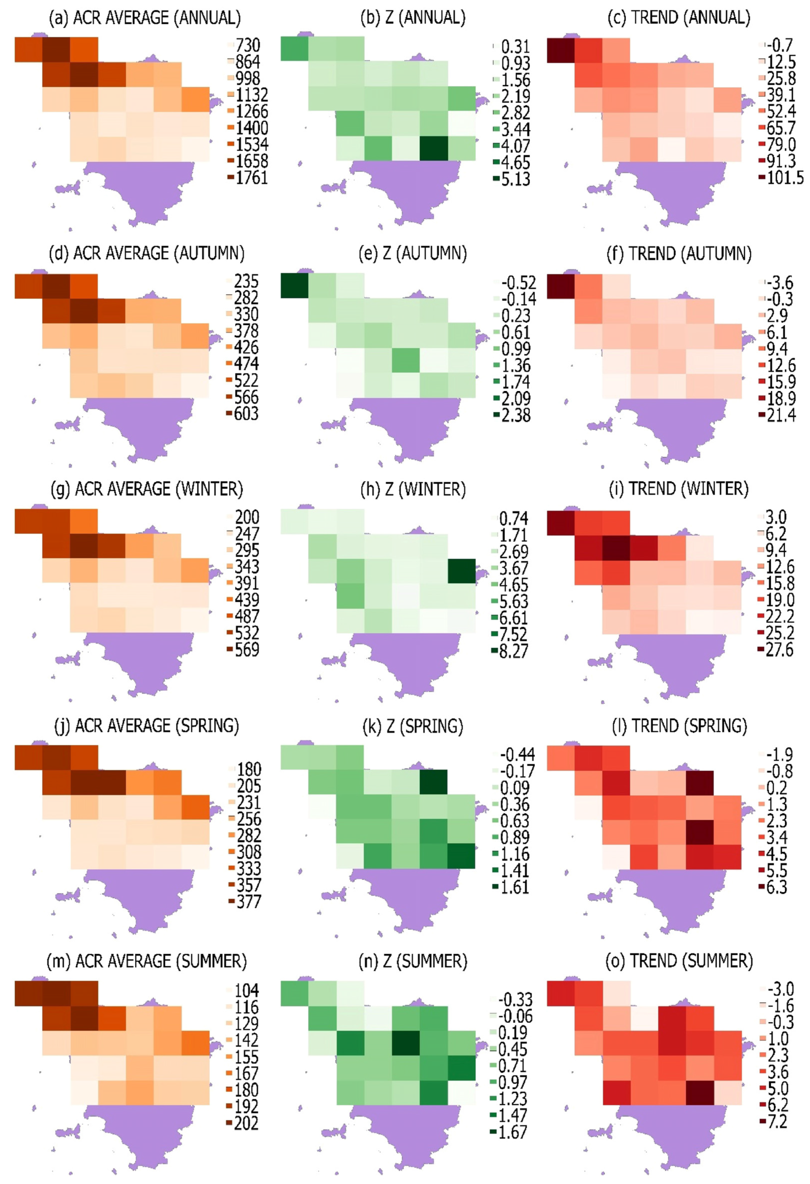
The annual and seasonal ACR_AV of each area was calculated (Equation (10)); the results are reported in Table 3 and Figure 6. The annual values of ACR_AV highlight different rainfall regimes for different areas. In central-southern areas (centered at lat. 43.21° and 43.48°) ACR_AV were between 800 and 900 mm, in central-northern areas (centered at lat. 43.75°) they were about 1000 mm. In north-western areas (centered at lat. 44.01°, 44.28° and lon. 10.12°, 10.87°) ACR_AV were about 1600 mm, in north-eastern areas (lat. 44.01°, lon. 11.25°, 11.62°) 1100 mm.
In spring, the ACR_AV values in central-southern areas were about 210 mm. In central-northern areas a gradient in the east–west direction was observed; in the east, the ACR values were about 200 mm, while in the west 280 mm. In north-western areas, they were about 350 mm, while in north-eastern areas 300 mm. In the summer, the ACR_AV values in central-southern and central-northern areas were about 130 mm, and in northern areas 200 mm. In autumn, in central-southern areas, a gradient in the east–west direction was observed; in the west, the ACR_AV values were about 350 mm, in the east 250 mm. In central-northern and northern areas, values were about 350 mm and 500 mm respectively. In the winter, the ACR_AV values in central-southern areas were about 250 mm, in central-northern areas about 300 mm and 500 mm in northern areas.
Based on these results, it may be noted that the annual volume of rainfall decreases moving in the north–south direction; furthermore, the north-western part of the territory was rainier than the north-east. The rainfall regime, on a seasonal basis, reproduces the same pattern; if a region is rainier annually, the same pattern occurs for all seasons.
3.3.2. Evolution of the Local Rainfall Regime
The trend analysis was performed for the time series of annual and seasonal ACR of each area (Figure 2 and Figure 6, Table 3). For almost all areas, the value of the Z statistic of the Mann–Kendall test was positive, which is a clue to a positive trend. The Z value of many time series was lower than 1.96, the threshold chosen to reject the null hypothesis, therefore it is not possible to state with sufficient confidence the presence of a positive trend in many of the areas considered.
The magnitude of trends of annual ACR was higher in the north-western coastal areas; in general the gradient of the trend magnitude was directed towards the north-west; in other words, there is a trend increase by moving in the western and northern directions. The typical trend magnitude was some tens of mm/year. In autumn, winter and summer, the trend analysis highlights a similar pattern to the annual one; in spring, the magnitude of the trend was overall homogeneous.
3.4. Characterization of the Global Rainfall Regime
The annual and seasonal values of ACR_TOT, NRD, MIP, SD0, SD10, SD25, SD40 were evaluated (Figure 7 and Figure 8). The Mann–Kendall test was performed for all time series (Table 4).
ACR_TOTann highlights an increase in precipitation; the Z statistic value of 1.86 was very close to the threshold value, suggesting the presence of a growing trend. The trend magnitude of 35.4 mm/year indicates a significant increase in the rainfall amount. The Z values of ACR_TOTaut, ACR_TOTwin, ACR_TOTspr, ACR_TOTsum show an increase in precipitation only in winter.
The trend analysis of the NRDann time series does not clearly highlight an increase in this observable. However, the Z values of seasonal time series show that a positive trend was detected only in winter.
The Z value of MIPann was 1.86; also in this case, the presence of a positive trend is very likely. The analysis of the Z statistic of the seasonal time series did not show an increase in this observable; although the Z value of MIPwin suggests the possible presence of a positive trend in winter.
The study of these observables highlights that one of the causes of the increase in annual precipitation was the growth of MIPann. The Mann–Kendall test of NRDann does not clearly show a positive trend, although the Z value might suggest it; therefore, it cannot be excluded that this phenomenon could also have caused the increase in annual rainfall. For all the considered time series, the positive trend was always attributable to a change of the rainfall regime in winter; a clear growth of the observables was not highlighted in the other seasons.
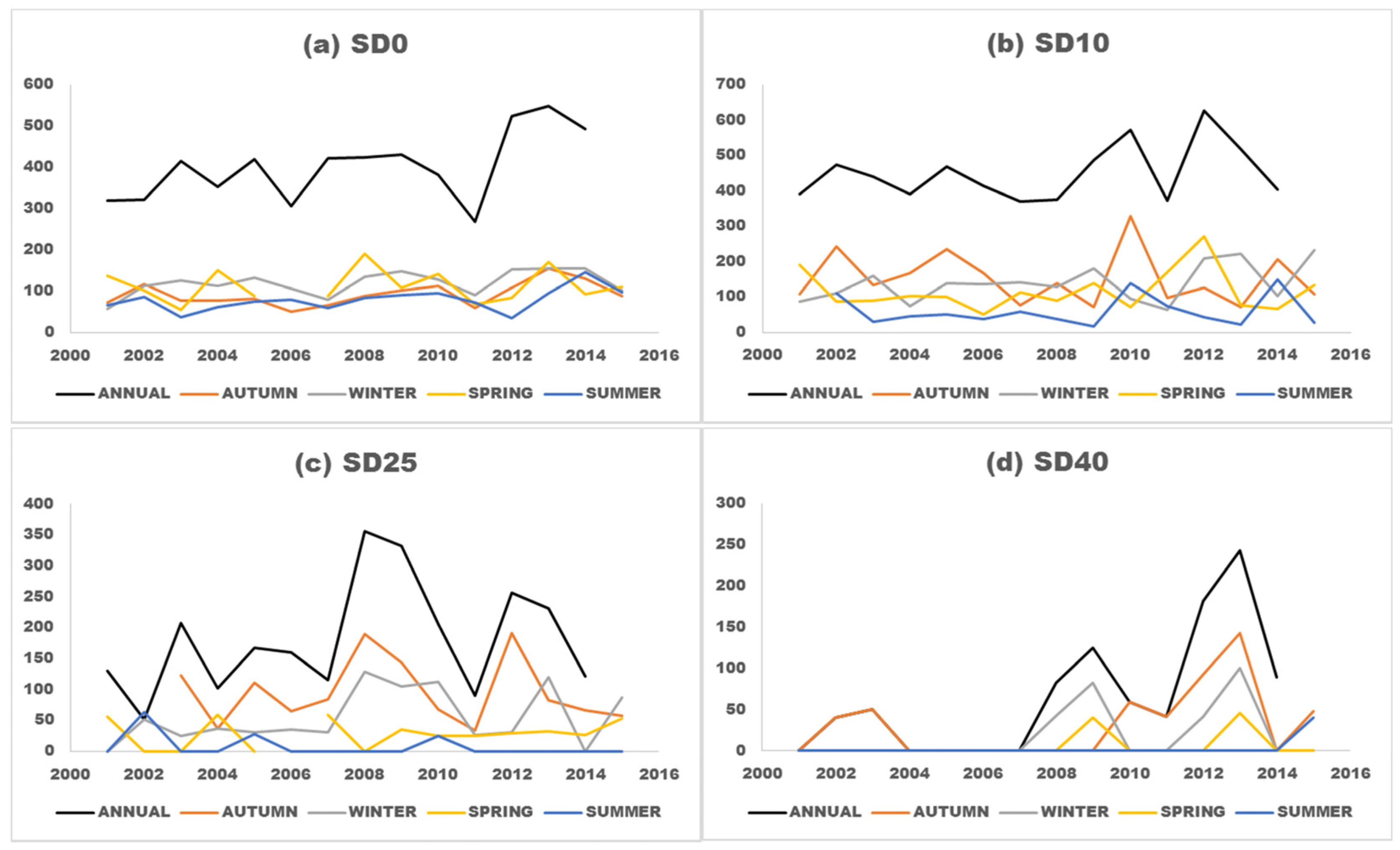
The trend analysis of SD0ann shows a positive trend; the value of the Z statistic was 2.36. The magnitude of trend equal to 13.3 mm/year was very high, so the rainfall amount caused by low-intensity events has increased a lot during the considered period. SD10ann and SD25ann did not show any positive trend, so the rainfall amount due to medium intensity events can be considered stationary. The value of the Z statistic of SD40ann was 2.58, so the presence of a positive trend was established. The magnitude of the trend equal to 10.5 mm/year was very high; it shows a significant increase in the contribution of extreme events to the rainfall amount.
The analysis of seasonal time series shows that the rainfall regime in autumn, winter and summer was similar to the annual one; there was an increase in rainfall amount for the light and extreme precipitations and there was substantial stability for the intermediate ones. In the spring, no trend was observed in any of the intensity groups.
4. Discussion and Conclusions
The estimation of rainfall amount is fundamental to evaluate the rainfall regime on the territory. The observable introduced to perform this task was the ACR [13,14], evaluated on some square areas in the studied territory. In addition to the best value of the observable, it is very important to quantitatively evaluate the uncertainty to establish the validity of the results. The annual and seasonal ACR and its uncertainty was therefore estimated, spatializing the measurements of a rain gauge network by means of the NPOBK technique [13,14,15,16,17,18]. The daily measurements were evaluated without an assessment of the error.
The uncertainty was due mainly to the limited density of rain gauges on the territory; indeed, the standard deviation of the ACR estimate depends essentially on the number of rain gauges in the area. In this context, a compromise was reached about the size of the square areas (30 × 30 km2) that allows a satisfactory spatial resolution and an acceptable uncertainty. Only the northern and central part of Tuscany was studied as the low density of rain gauges in the south does not allow acceptable estimates to be obtained. The period considered was 1 March 2001–31 May 2016.
The results can be summarized as follows:
the territory can be divided into four areas distinguished by the ACR_AV values during the considered period. The north-western area is the rainiest (ACR_AV about 1600 mm) and experienced the highest increase in precipitation. The north-eastern area (ACR_AV about 1200 mm), central area (ACR_AV about 1000 mm) and southern-central area (ACR_AV about 800 mm) had the most limited increase in precipitation. For all areas, the precipitation in autumn and winter was more abundant than in spring; summer precipitation was the least abundant.
The ACR_TOT time series showed a very strong increase in precipitation; this was assessed as 35 mm/year and was mainly due to winter rainfall. It was caused by the positive trend in MIP and probably also in NRD. The ACR_TOT positive trend was not homogenous on the territory but the magnitude of the trend was higher in the north-western area. Analysis of the distribution of daily precipitation shows an increase in the contribution of low and extreme intensity events, while the contribution of medium intensity events can be considered stationary.
The increase in rainfall that occurred during the considered period is in contrast with the overall trend of the last decades. Bartolini et al. [23] showed a tendency to a decrease in rainfall during the period 1948–2009 in two distinct sites in Tuscany, while Fatichi et al. [22], during the period 1916–2003, showed an absence of any trends in precipitation amount or intensity of extreme events.
The results of this paper are only apparently surprising. Within a generally decreasing rainfall trend, a period of precipitation increase may occur without affecting the overall trend. For example, Romano et al. [28] showed an overall decreasing trend in annual precipitation in the Tiber river basin, an area close to Tuscany. The details of the pattern of the rainfall time series showed a succession of dry and wet periods when the rainfall amount increased.
The values of SD40 have increased, so extreme rainfall events have become more frequent. This result is in agreement with Crisci et al. [29] who reported an increase of extreme events in Tuscany during the period 1973–1994, while Fatichi et al. [22] did not detect any trend on the basis of a longer time series. The increase in extreme precipitation aggravates the risk of flooding; in this context, the monitoring of these events, also with the technique described in this paper, becomes essential.
In the future, the ACR estimates will be improved by means of the measurements from radar operating on the territory. The radar can measure the average rain rate on 1 × 1 km square pixels, so can improve the spatial resolution of ACR estimates. The radar sweeps all Tuscany, so the measurements will allow the rainfall regime to be studied over the whole region.
Acknowledgments
The Tuscany region meteorological network managed by the Hydrological Service of Tuscany provided rain gauge data.
Conflicts of Interest
The author declares no conflict of interest.
References
- Trenberth, K.E.; Dai, A.; Rasmussen, R.M.; Parsons, D.B. The changing character of precipitation. Bull. Am. Meteorol. Soc. 2003, 84, 1205–1217. [Google Scholar] [CrossRef]
- Brunetti, M.; Maugeri, M.; Monti, F.; Nanni, T. Temperature and precipitation variability in Italy in the last two centuries from homogenised instrumental time series. Int. J. Climatol. 2006, 26, 345–381. [Google Scholar] [CrossRef]
- Romero, R.; Guijarro, J.A.; Ramis, C.; Alonso, S. A 30-year (1964–1993) daily rainfall data base for the Spanish Mediterranean regions: First exploratory study. Int. J. Climatol. 1998, 18, 541–560. [Google Scholar] [CrossRef]
- Alpert, P. The paradoxical increase of Mediterranean extreme daily rainfall in spite of decrease in total values. Geophys. Res. Lett. 2002, 29, 31.1–31.4. [Google Scholar] [CrossRef]
- Brunetti, M.; Maugeri, M.; Nanni, T. Changes in total precipitation, rainy days and extreme events in northeastern Italy. Int. J. Climatol. 2001, 21, 861–871. [Google Scholar] [CrossRef]
- Martínez, M.D.; Lana, X.; Burgueño, A.; Serra, C. Spatial and temporal daily rainfall regime in Catalonia (NE Spain) derived from four precipitation indices, years 1950–2000. Int. J. Climatol. 2007, 27, 123–138. [Google Scholar] [CrossRef]
- Brunetti, M.; Colacino, M.; Maugeri, M.; Nanni, T. Trends in the daily intensity of precipitation in Italy from 1951 to 1996. Int. J. Climatol. 2001, 21, 299–316. [Google Scholar] [CrossRef]
- Jang, J.H. An advanced method to apply multiple rainfall thresholds for urban flood warnings. Water 2015, 7, 6056–6078. [Google Scholar] [CrossRef]
- Notaro, V.; Liuzzo, L.; Freni, G.; La Loggia, G. Uncertainty analysis in the evaluation of extreme rainfall trends and its implications on urban drainage system design. Water 2015, 7, 6931–6945. [Google Scholar] [CrossRef]
- Pedersen, L.; Jensen, N.E.; Christensen, L.E.; Madsen, H. Quantification of the spatial variability of rainfall based on a dense network of rain gauges. Atmos. Res. 2010, 95, 441–454. [Google Scholar] [CrossRef]
- Mandapaka, P.V.; Krajewski, W.F.; Ciach, G.J.; Villarini, G.; Smith, J.A. Estimation of radar-rainfall error spatial correlation. Adv. Water Resour. 2009, 32, 1020–1030. [Google Scholar] [CrossRef]
- Ciach, G.J.; Krajewski, W.F. On the estimation of radar rainfall error variance. Adv. Water Resour. 1999, 22, 585–595. [Google Scholar] [CrossRef]
- Mazza, A.; Antonini, A.; Melani, S.; Ortolani, A. Recalibration of cumulative rainfall estimates by weather radar over a large area. J. Appl. Remote Sens. 2015, 9, 095993. [Google Scholar] [CrossRef]
- Mazza, A.; Antonini, A.; Melani, S.; Ortolani, A. Estimates of cumulative rainfall over a large area by weather radar. In Proceedings of the SPIE Remote Sensing and Security, Remote Sensing of Clouds and the Atmosphere XIX and Optics in Atmospheric Propagation and Adaptive Systems XVII, Amsterdam, The Netherlands, 22–25 September 2014.
- Chiles, J.P.; Delfiner, P.B. Structural analysis. In Geostatistics: Modeling Spatial Uncertainty, 2nd ed.; Balding, D.J., Cressie, N.A., Eds.; John Wiley & Sons: Hoboken, NJ, USA, 2012; pp. 28–146. [Google Scholar]
- Chiles, J.P.; Delfiner, P.B. Kriging. In Geostatistics: Modeling Spatial Uncertainty, 2nd ed.; Balding, D.J., Cressie, N.A., Eds.; John Wiley & Sons: Hoboken, NJ, USA, 2012; pp. 147–237. [Google Scholar]
- Wackemagel, H. Geostatistics. In Multivariate. Geostatistics an Introduction with Applications, 3rd ed.; Springer: Berlin, Germany, 2003; pp. 35–120. [Google Scholar]
- Armstrong, M. The theory of kriging. In Basic Linear Geostatistics, 1st ed.; Springer: Berlin, Germany, 1998; pp. 83–102. [Google Scholar]
- Doneaud, A.; Ionescu-Niscov, S.; Priegnitz, D.L.; Smith, P.L. The area-time integral as an indicator for convective rain volumes. J. Clim. Appl. Meteorol. 1984, 23, 555–561. [Google Scholar] [CrossRef]
- Doneaud, A.A.; Smith, P.L.; Dennis, A.S.; Sengupta, S. A simple method for estimating convective rain volume over an area. Water Resour. Res. 1981, 17, 1676–1682. [Google Scholar] [CrossRef]
- Griffith, C.G.; Woodley, W.L.; Grube, P.G.; Martin, D.W.; Stout, J.; Sikdar, D.N. Rain estimation from geosynchronous satellite imagery—Visible and infrared studies. Mon. Weather Rev. 1978, 106, 1153–1171. [Google Scholar] [CrossRef]
- Fatichi, S.; Caporali, E. A comprehensive analysis of changes in precipitation regime in Tuscany. Int. J. Climatol. 2009, 29, 1883–1893. [Google Scholar] [CrossRef]
- Bartolini, G.; Grifoni, D.; Torrigiani, T.; Vallorani, R.; Meneguzzo, F.; Gozzini, B. Precipitation changes from two long-term hourly datasets in Tuscany, Italy. Int. J. Climatol. 2014, 34, 3977–3985. [Google Scholar] [CrossRef]
- Hamed, K.H.; Ramachandra Rao, A. A modified Mann-Kendall trend test for autocorrelated data. J. Hydrol. 1998, 204, 182–196. [Google Scholar] [CrossRef]
- Hipel, K.W.; McLeod, A.I. Non parametric test for trend detection. In Time Series Modelling of Water Resources and Environmental Systems, 1st ed.; Elsevier: Amsterdam, The Netherlands, 1994; pp. 853–938. [Google Scholar]
- Sen, P.K. Estimates of the regression coefficient based on Kendall’s Tau. J. Am. Stat. Assoc. 1968, 63, 1379–1389. [Google Scholar] [CrossRef]
- Qu, B.; Lv, A.; Jia, S.; Zhu, W. Daily precipitation changes over large river basins in China. 1960–2013. Water 2016, 8, 185. [Google Scholar] [CrossRef]
- Romano, E.; Preziosi, E. Precipitation pattern analysis in the Tiber River basin (central Italy) using standardized indices. Int. J. Climatol. 2013, 33, 1781–1792. [Google Scholar] [CrossRef]
- Crisci, A.; Gozzini, B.; Meneguzzo, F.; Pagliara, S.; Maracchi, G. Extreme rainfall in a changing climate: Regional analysis and hydrological implications in Tuscany. Hydrol. Process. 2002, 16, 1261–1274. [Google Scholar] [CrossRef]
Figure 1.
The Tuscany rain gauge network. (a) shows the position of the Tuscany region on the Italian peninsula; (b) the rain gauges installed in the region (March 2015).
Figure 1.
The Tuscany rain gauge network. (a) shows the position of the Tuscany region on the Italian peninsula; (b) the rain gauges installed in the region (March 2015).
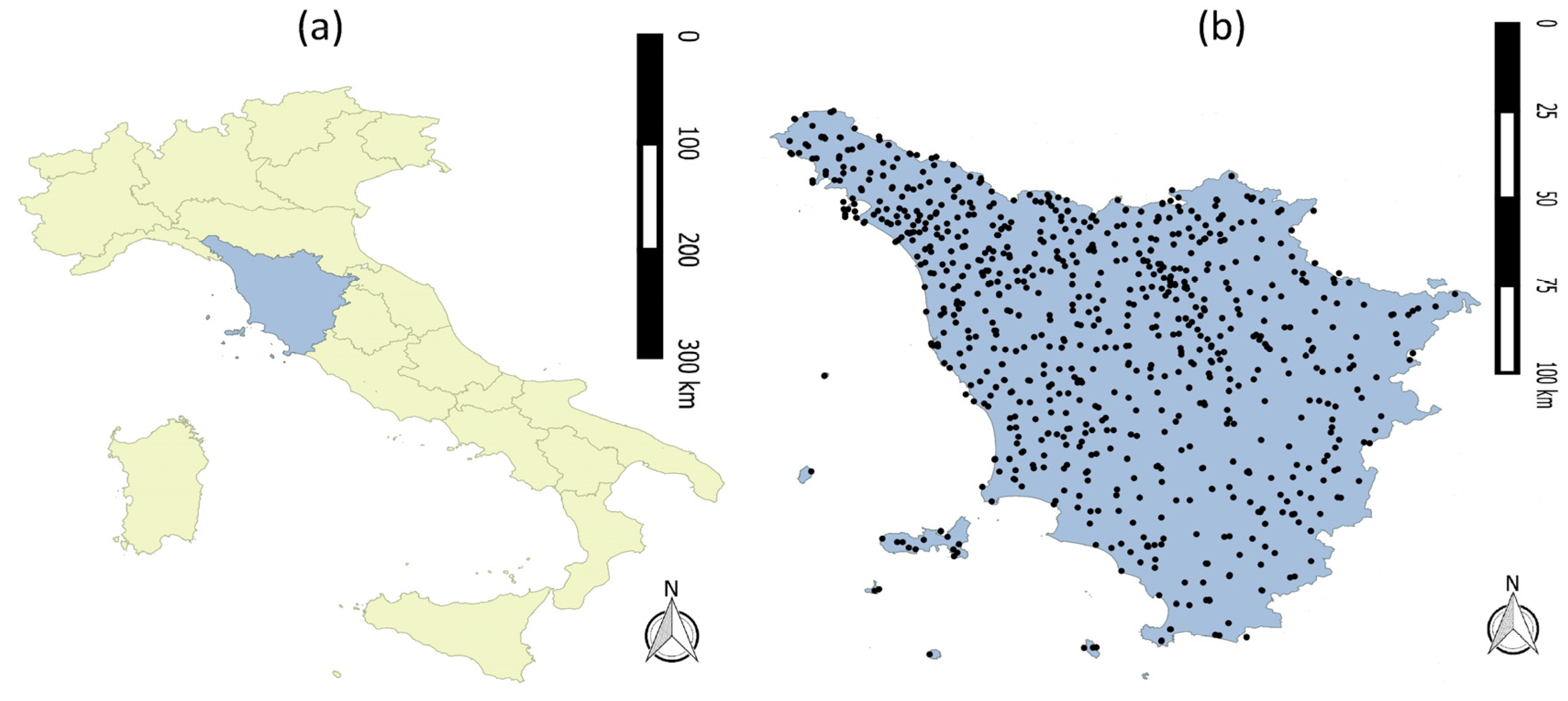
Figure 2.
Areas where the ACR was estimated. Latitude and longitude of the centers of the areas expressed in decimal degrees are indicated below and above them.
Figure 2.
Areas where the ACR was estimated. Latitude and longitude of the centers of the areas expressed in decimal degrees are indicated below and above them.
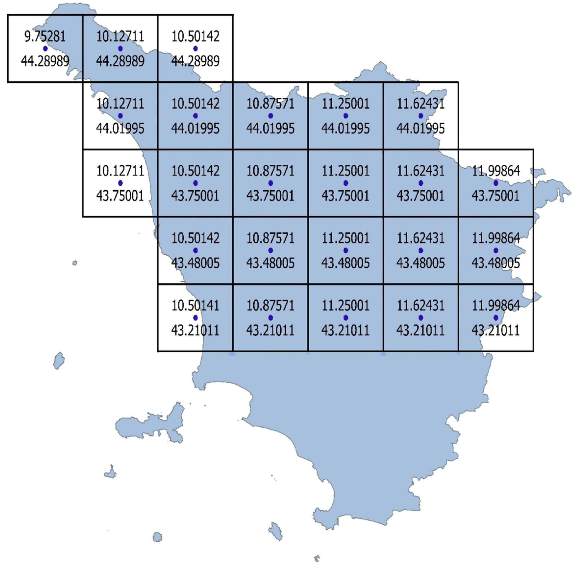
Figure 3.
Variograms of annual (a) and seasonal (b–e) ACR (year: 2009–2010, areas centered at lat. 43.75°, lon. 11.25°). The sample values obtained with the measurements inside 50 × 50, 60 × 60, and 70 × 70 km2 areas are reported. The distances of the points (meters) are reported in the abscissa, the values of the variogram (mm2) in the ordinate. The fitting function is also reported.
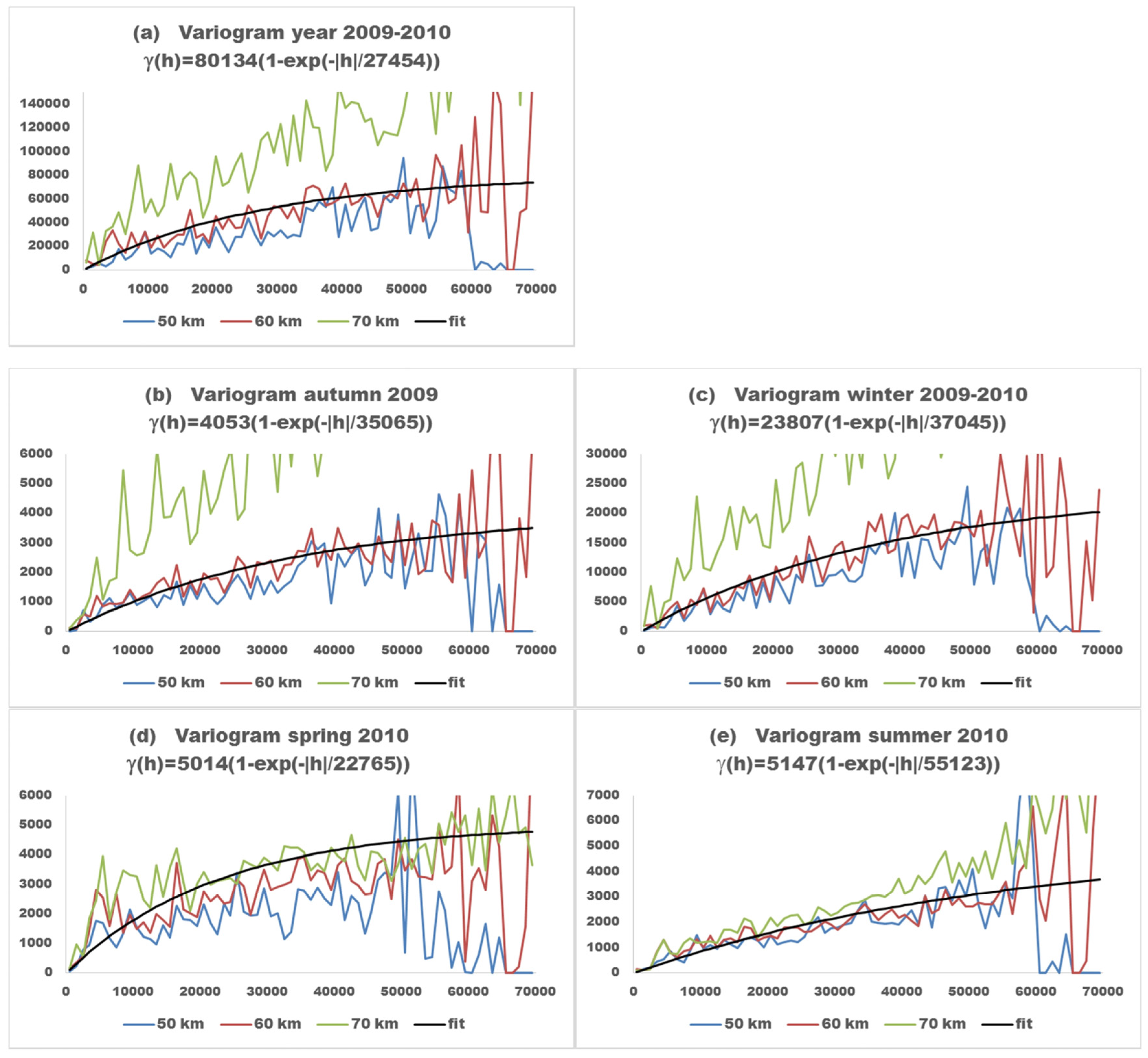
Figure 4.
Annual (a) and seasonal (c,e,g,i) ACR (mm) and their relative errors (b,d,f,h,j), for all areas, year: 2003–2004.
Figure 4.
Annual (a) and seasonal (c,e,g,i) ACR (mm) and their relative errors (b,d,f,h,j), for all areas, year: 2003–2004.
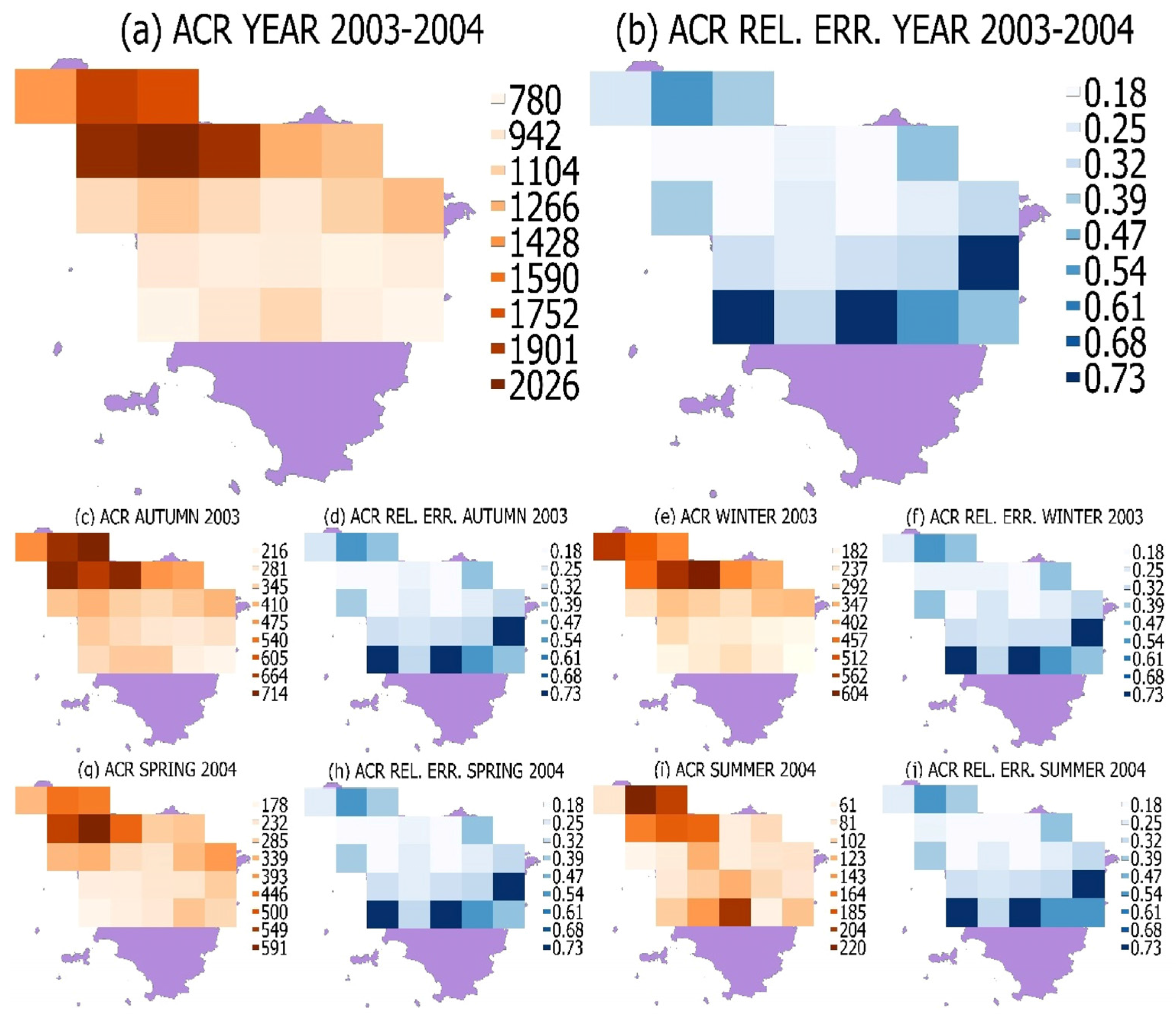
Figure 5.
Annual (a) and seasonal (c,e,g,i) ACR (mm) and their relative errors (b,d,f,h,j), for all areas, year: 2014–2015.
Figure 5.
Annual (a) and seasonal (c,e,g,i) ACR (mm) and their relative errors (b,d,f,h,j), for all areas, year: 2014–2015.
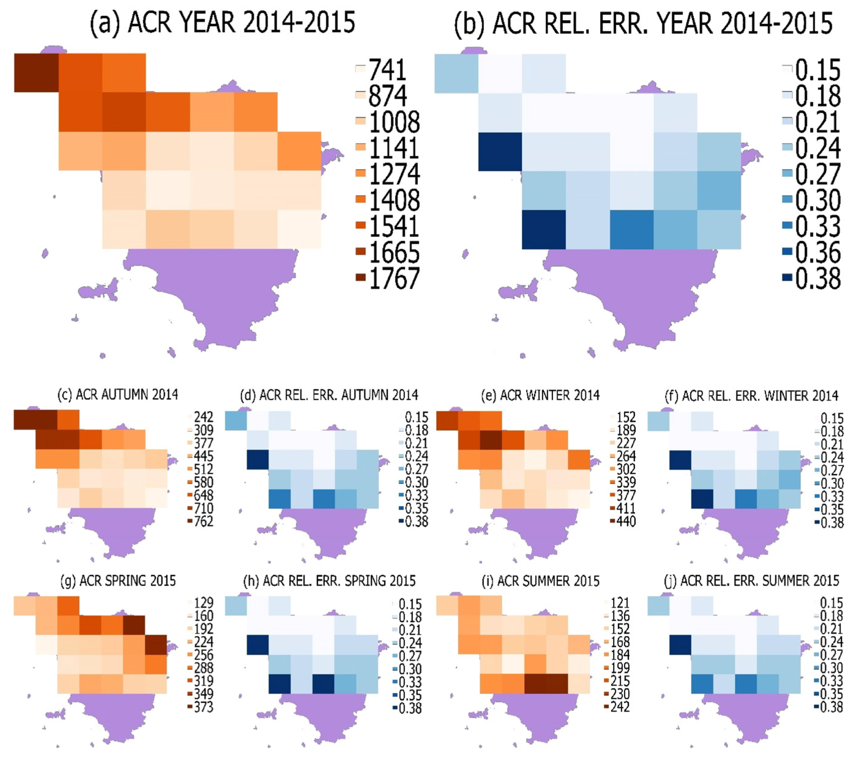
Figure 6.
Annual and seasonal ACR_AV estimates (a,d,g,j,m); values of Z statistic (b,e,h,k,n); and magnitudes of the trend (c,f,i,l,o).
Figure 6.
Annual and seasonal ACR_AV estimates (a,d,g,j,m); values of Z statistic (b,e,h,k,n); and magnitudes of the trend (c,f,i,l,o).

Figure 7.
Annual and seasonal time series of ACR_TOT (a); NRD (b) and MIP (c).
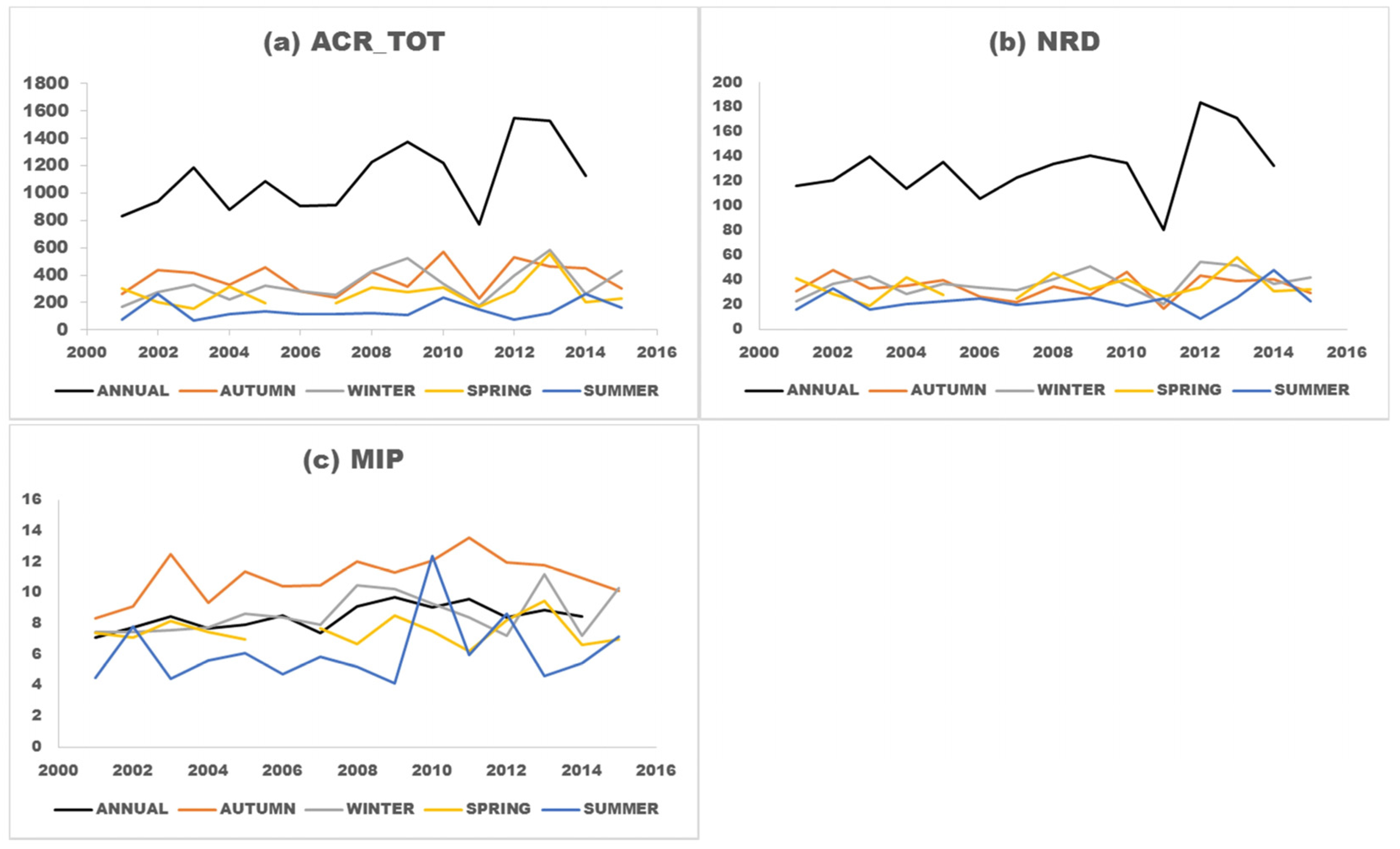
Figure 8.
Annual and seasonal time series of SD0 (a); SD10 (b); SD25 (c) and SD40 (d).


Table 1.
Examples of annual and seasonal ACR (mm) and their standard deviations (σ) and relative errors (ERR). M denotes missing values. Latitude and longitude are expressed in decimal degrees.
| lat.: 43.480053 lon.: 11.250000 | |||||||||||||||
| YEAR | ANNUAL | AUTUMN | WINTER | SPRING | SUMMER | ||||||||||
| ACR | σ | ERR | ACR | σ | ERR | ACR | σ | ERR | ACR | σ | ERR | ACR | σ | ERR | |
| 2001–2002 | 795 | 99 | 0.38 | 229 | 29 | 0.38 | 117 | 17 | 0.43 | 197 | 25 | 0.38 | 172 | 43 | 0.75 |
| 2002–2003 | 780 | 80 | 0.31 | 290 | 30 | 0.31 | 238 | 24 | 0.31 | 158 | 16 | 0.31 | 104 | 26 | 0.75 |
| 2003–2004 | 870 | 89 | 0.31 | 278 | 28 | 0.31 | 238 | 24 | 0.31 | 227 | 23 | 0.31 | 208 | 52 | 0.75 |
| 2004–2005 | 798 | 89 | 0.34 | 143 | 36 | 0.75 | 222 | 25 | 0.34 | 158 | 18 | 0.34 | 226 | 57 | 0.75 |
| 2005–2006 | 983 | 110 | 0.34 | 513 | 57 | 0.34 | 220 | 25 | 0.34 | M | M | M | 100 | 11 | 0.34 |
| 2006–2007 | 842 | 86 | 0.31 | 240 | 18 | 0.23 | 189 | 14 | 0.22 | 200 | 13 | 0.19 | 78 | 9 | 0.34 |
| 2007–2008 | 681 | 51 | 0.23 | 135 | 11 | 0.25 | 188 | 14 | 0.23 | 224 | 16 | 0.22 | 109 | 11 | 0.31 |
| 2008–2009 | 931 | 95 | 0.31 | 324 | 23 | 0.22 | 272 | 17 | 0.19 | 221 | 14 | 0.19 | 139 | 14 | 0.31 |
| 2009–2010 | 982 | 61 | 0.19 | 200 | 13 | 0.19 | 365 | 23 | 0.19 | 265 | 15 | 0.17 | 96 | 10 | 0.31 |
| 2010–2011 | 937 | 60 | 0.19 | 443 | 30 | 0.20 | 230 | 15 | 0.19 | 123 | 8 | 0.19 | 138 | 14 | 0.31 |
| 2011–2012 | 541 | 36 | 0.20 | 127 | 8 | 0.20 | 114 | 8 | 0.21 | 224 | 15 | 0.20 | 64 | 6 | 0.28 |
| 2012–2013 | 1155 | 83 | 0.22 | 446 | 31 | 0.21 | 261 | 19 | 0.22 | 309 | 21 | 0.20 | 136 | 34 | 0.75 |
| 2013–2014 | 1266 | 95 | 0.23 | 418 | 29 | 0.21 | 330 | 24 | 0.22 | 170 | 13 | 0.23 | 233 | 41 | 0.53 |
| 2014–2015 | 824 | 51 | 0.19 | 316 | 19 | 0.18 | 203 | 12 | 0.18 | 176 | 10 | 0.18 | 246 | 27 | 0.34 |
| lat.: 44.019947 lon.: 10.875702 | |||||||||||||||
| YEAR | ANNUAL | AUTUMN | WINTER | SPRING | SUMMER | ||||||||||
| ACR | σ | ERR | ACR | σ | ERR | ACR | σ | ERR | ACR | σ | ERR | ACR | S | ERR | |
| 2001–2002 | 1375 | 243 | 0.53 | 386 | 97 | 0.75 | 284 | 35 | 0.38 | 324 | 21 | 0.19 | 359 | 24 | 0.20 |
| 2002–2003 | 1434 | 96 | 0.20 | 750 | 48 | 0.19 | 408 | 27 | 0.20 | 194 | 13 | 0.21 | 63 | 5 | 0.22 |
| 2003–2004 | 1940 | 130 | 0.20 | 701 | 47 | 0.20 | 617 | 45 | 0.22 | 464 | 31 | 0.20 | 171 | 11 | 0.19 |
| 2004–2005 | 1036 | 116 | 0.34 | M | M | M | 251 | 17 | 0.20 | 291 | 19 | 0.19 | 194 | 20 | 0.31 |
| 2005–2006 | 1459 | 94 | 0.19 | 509 | 33 | 0.19 | 490 | 33 | 0.20 | M | M | M | 199 | 11 | 0.17 |
| 2006–2007 | 1328 | 83 | 0.19 | 364 | 21 | 0.17 | 504 | 29 | 0.17 | 251 | 14 | 0.16 | 159 | 10 | 0.18 |
| 2007–2008 | 1231 | 71 | 0.17 | 341 | 20 | 0.17 | 353 | 20 | 0.17 | 427 | 23 | 0.16 | 105 | 6 | 0.16 |
| 2008–2009 | 1843 | 109 | 0.18 | 677 | 37 | 0.16 | 700 | 37 | 0.16 | 392 | 21 | 0.16 | 111 | 6 | 0.15 |
| 2009–2010 | 1906 | 97 | 0.15 | 453 | 23 | 0.15 | 786 | 39 | 0.15 | 361 | 18 | 0.15 | 317 | 16 | 0.15 |
| 2010–2011 | 1744 | 89 | 0.15 | 740 | 38 | 0.15 | 575 | 29 | 0.15 | 233 | 11 | 0.15 | 210 | 10 | 0.15 |
| 2011–2012 | 1162 | 59 | 0.15 | 384 | 20 | 0.15 | 287 | 15 | 0.16 | 424 | 21 | 0.15 | 80 | 4 | 0.15 |
| 2012–2013 | 2193 | 112 | 0.15 | 744 | 37 | 0.15 | 570 | 29 | 0.15 | 815 | 40 | 0.15 | 140 | 7 | 0.15 |
| 2013–2014 | 2241 | 117 | 0.16 | 599 | 31 | 0.15 | 1057 | 54 | 0.15 | 290 | 15 | 0.16 | 300 | 15 | 0.15 |
| 2014–2015 | 1478 | 75 | 0.15 | 643 | 33 | 0.15 | 374 | 19 | 0.15 | 325 | 17 | 0.15 | 138 | 7 | 0.15 |
| Lat. | Lon. | Day_Month_Year | ACR AM | ACR NPOBK |
|---|---|---|---|---|
| 43.75 | 10.13 | 11_11_2001 | 4.4 | 5.2 |
| 44.02 | 10.88 | 7_10_2003 | 0.8 | 0.5 |
| 44.02 | 10.13 | 29_10_2004 | 44.1 | 37.0 |
| 44.29 | 9.75 | 22_3_2006 | 12.2 | 8.9 |
| 44.20 | 10.13 | 29_2_2008 | 1.2 | 1.9 |
| 43.75 | 12.00 | 24_7_2011 | 7.5 | 11.0 |
| 43.21 | 11.25 | 5_10_2013 | 17.1 | 18.7 |
Table 3.
Annual and seasonal ACR_AV estimates, values of Z statistic and magnitudes of the trend. The Z values >1.96 are reported in bold.
| ANNUAL | AUTUMN | WINTER | SPRING | SUMMER | ||||||||||||
|---|---|---|---|---|---|---|---|---|---|---|---|---|---|---|---|---|
| Lat | Lon | ACR AV | Z | T | ACR AV | Z | T | ACR AV | Z | T | ACR AV | Z | T | ACR AV | Z | T |
| 43.21 | 10.50 | 914 | 1.17 | 23.1 | 335 | −0.48 | −3.6 | 269 | 1.89 | 7.9 | 202 | −0.21 | −1.8 | 104 | 0.62 | 5.2 |
| 43.21 | 10.88 | 955 | 3.09 | 34.3 | 350 | 0.06 | −0.1 | 284 | 3.03 | 9.5 | 210 | 0.99 | 3.5 | 136 | 0.44 | 2.6 |
| 43.21 | 11.25 | 870 | 0.95 | −0.7 | 329 | −0.22 | −1.8 | 249 | 1.31 | 7.0 | 199 | 0.43 | 0.8 | 146 | 0.33 | 2.5 |
| 43.21 | 11.62 | 827 | 5.28 | 20.9 | 273 | 0.44 | 1.1 | 229 | 0.74 | 3.0 | 196 | 0.99 | 4.7 | 130 | 1.31 | 7.6 |
| 43.21 | 12.00 | 730 | 2.01 | 13.3 | 235 | 0.22 | 0.6 | 200 | 0.90 | 3.5 | 180 | 1.48 | 4.3 | 129 | −0.33 | −1.4 |
| 43.48 | 10.50 | 910 | 3.02 | 28.1 | 343 | −0.52 | −2.5 | 268 | 4.70 | 10.7 | 205 | 0.59 | 1.8 | 109 | 0.55 | 1.6 |
| 43.48 | 10.88 | 824 | 1.64 | 23.3 | 289 | 0.11 | 1.5 | 235 | 2.24 | 8.4 | 203 | 0.59 | 2.4 | 113 | 0.55 | 2.6 |
| 43.48 | 11.25 | 885 | 1.42 | 19.6 | 290 | 1.12 | 2.2 | 234 | 0.89 | 6.3 | 213 | 0.40 | 1.6 | 139 | 0.66 | 3.4 |
| 43.48 | 11.62 | 838 | 2.31 | 15.8 | 293 | −0.44 | −1.6 | 236 | 1.90 | 6.0 | 215 | 1.09 | 6.6 | 123 | 0.99 | 1.4 |
| 43.48 | 12.00 | 852 | 0.31 | 3.4 | 288 | −0.11 | −2.0 | 239 | 1.82 | 6.8 | 222 | 0.43 | 2.2 | 124 | 1.40 | 3.1 |
| 43.75 | 10.13 | 956 | 1.75 | 30.2 | 352 | −0.32 | 0.3 | 279 | 2.67 | 16.6 | 203 | −0.44 | −1.9 | 123 | 0.00 | 1.3 |
| 43.75 | 10.50 | 1075 | 1.75 | 40.6 | 380 | 0.32 | 2.0 | 339 | 4.22 | 19.6 | 242 | 0.69 | 3.3 | 135 | 1.31 | 3.2 |
| 43.75 | 10.88 | 896 | 1.86 | 37.8 | 292 | 0.55 | 3.2 | 270 | 2.35 | 9.3 | 210 | 0.69 | 2.9 | 133 | 0.55 | 3.2 |
| 43.75 | 11.25 | 841 | 2.08 | 19.1 | 286 | 0.10 | 1.3 | 242 | 1.39 | 9.5 | 201 | 0.30 | 2.6 | 132 | 1.73 | 5.4 |
| 43.75 | 11.62 | 1079 | 2.01 | 11.2 | 351 | 0.10 | 1.0 | 318 | 1.66 | 7.0 | 268 | 0.20 | 1.1 | 148 | 0.89 | 4.3 |
| 43.75 | 12.00 | 1264 | 2.87 | 35.3 | 402 | 0.44 | 3.6 | 371 | 8.50 | 9.3 | 317 | 0.30 | 2.1 | 166 | 0.66 | 3.2 |
| 44.02 | 10.13 | 1652 | 1.40 | 60.4 | 565 | 0.33 | 7.1 | 523 | 3.39 | 24.3 | 354 | 0.58 | 1.9 | 192 | 0.88 | 3.3 |
| 44.02 | 10.50 | 1777 | 1.65 | 52.1 | 614 | 0.18 | 3.0 | 580 | 1.98 | 28.4 | 383 | 0.66 | 4.8 | 202 | 0.00 | 0.2 |
| 44.02 | 10.88 | 1598 | 1.31 | 44.2 | 557 | 0.11 | 2.0 | 533 | 1.68 | 24.7 | 378 | 0.00 | 0.1 | 182 | −0.22 | −3.0 |
| 44.02 | 11.25 | 1156 | 1.64 | 31.8 | 383 | 0.10 | 0.4 | 371 | 1.58 | 14.8 | 282 | 0.10 | 0.4 | 133 | 0.79 | 5.4 |
| 44.02 | 11.62 | 1113 | 1.31 | 29.6 | 378 | 0.22 | 2.8 | 313 | 1.85 | 5.0 | 301 | 1.68 | 6.5 | 146 | 0.95 | 3.7 |
| 44.29 | 9.75 | 1588 | 3.50 | 104.6 | 554 | 2.47 | 22.2 | 521 | 1.78 | 26.5 | 355 | 0.30 | 2.3 | 199 | 0.88 | 5.0 |
| 44.29 | 10.13 | 1792 | 1.99 | 70.8 | 608 | 0.43 | 8.7 | 522 | 1.31 | 19.7 | 369 | 0.33 | 4.2 | 205 | 0.34 | 3.9 |
| 44.29 | 10.50 | 1517 | 2.12 | 40.0 | 525 | −0.06 | −0.4 | 434 | 1.64 | 18.9 | 345 | 0.55 | 3.4 | 195 | −0.18 | −2.0 |
Table 4.
Values of Z statistic and trend magnitudes of annual and seasonal observables. The Z values > 1.96 are reported in bold.
| ANNUAL | AUTUMN | WINTER | SPRING | SUMMER | ||||||
|---|---|---|---|---|---|---|---|---|---|---|
| Z | T | Z | T | Z | T | Z | T | Z | T | |
| ACR_TOT | 1.86 | 35.4 | 0.49 | 2.9 | 3.57 | 14.8 | 0.20 | 1.1 | 1.48 | 3.9 |
| NRD | 1.20 | 2.2 | 0.00 | −0.1 | 3.37 | 1.1 | 0.69 | 0.4 | 1.14 | 0.5 |
| MIP | 1.86 | 0.1 | 1.29 | 0.2 | 1.58 | 0.1 | 0.00 | 0.0 | 0.79 | 0.1 |
| SD0 | 2.36 | 13.3 | 1.68 | 3.3 | 1.78 | 3.1 | 0.40 | 0.6 | 4.16 | 2.7 |
| SD10 | 0.71 | 4.3 | −0.79 | −1.6 | 1.48 | 6.5 | 0.10 | 0.5 | 0.40 | 1.7 |
| SD25 | 0.88 | 7.6 | 0.30 | 0.5 | 0.94 | 2.8 | 0.10 | 0.0 | −1.14 | 0.0 |
| SD40 | 2.58 | 10.5 | 1.51 | 0.2 | 3.96 | 2.689 | 0.68 | 0.0 | 1.50 | 0.0 |
© 2017 by the author. Licensee MDPI, Basel, Switzerland. This article is an open access article distributed under the terms and conditions of the Creative Commons Attribution (CC BY) license ( http://creativecommons.org/licenses/by/4.0/).
Share and Cite
MDPI and ACS Style
Mazza, A. Space–Time Characterization of Rainfall Field in Tuscany. Water 2017, 9, 86. https://doi.org/10.3390/w9020086
AMA Style
Mazza A. Space–Time Characterization of Rainfall Field in Tuscany. Water. 2017; 9(2):86. https://doi.org/10.3390/w9020086
Chicago/Turabian StyleMazza, Alessandro. 2017. "Space–Time Characterization of Rainfall Field in Tuscany" Water 9, no. 2: 86. https://doi.org/10.3390/w9020086
Note that from the first issue of 2016, this journal uses article numbers instead of page numbers. See further details here.