Examining the Relationship between Drought Indices and Groundwater Levels


Abstract
:1. Introduction
2. Study Area and Methods
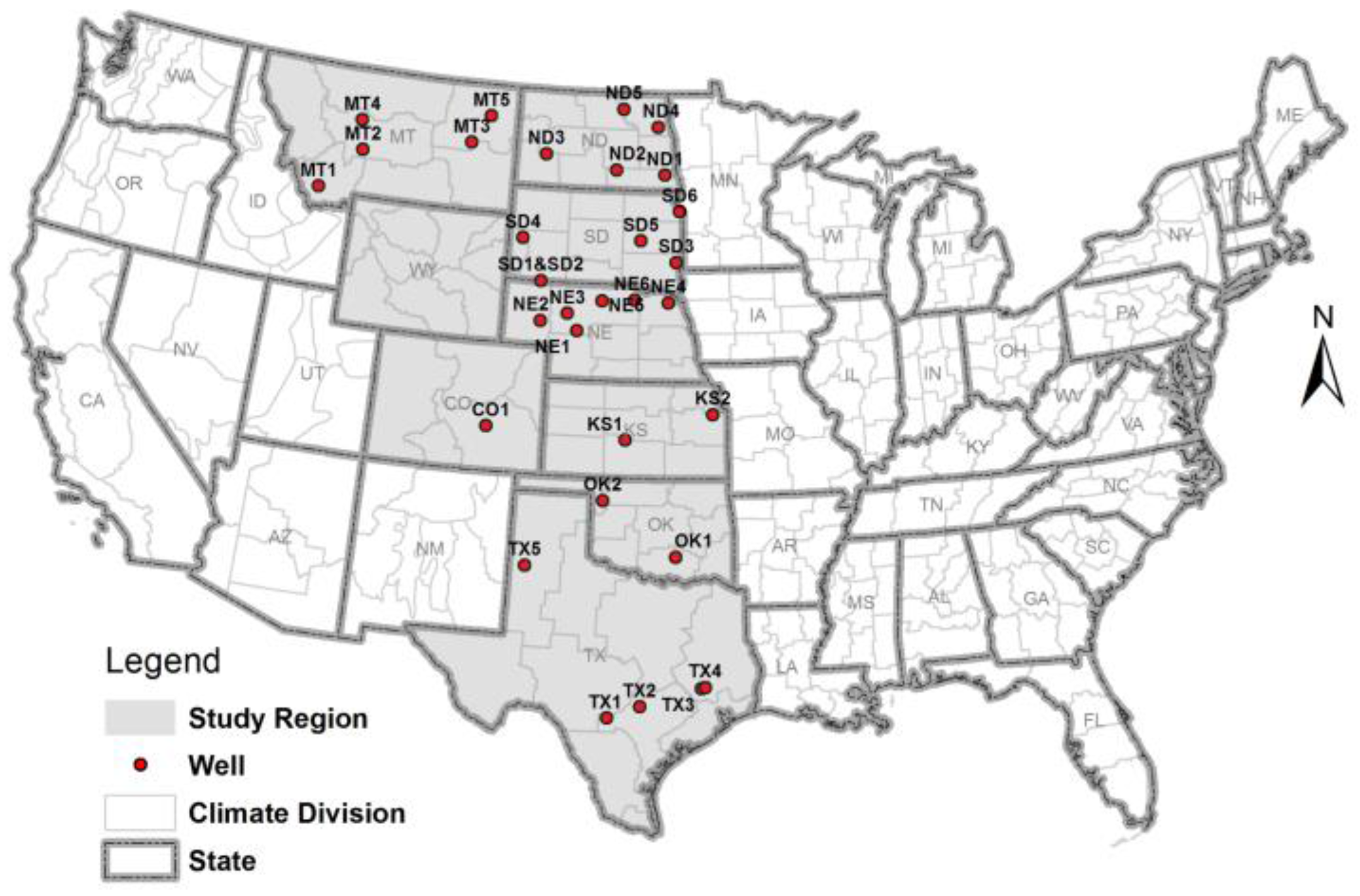
2.1. Study Area and Groundwater Levels Data
2.2. Drought Indices
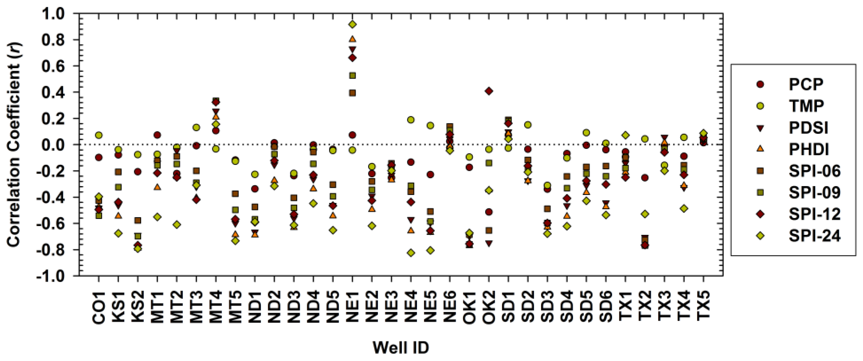
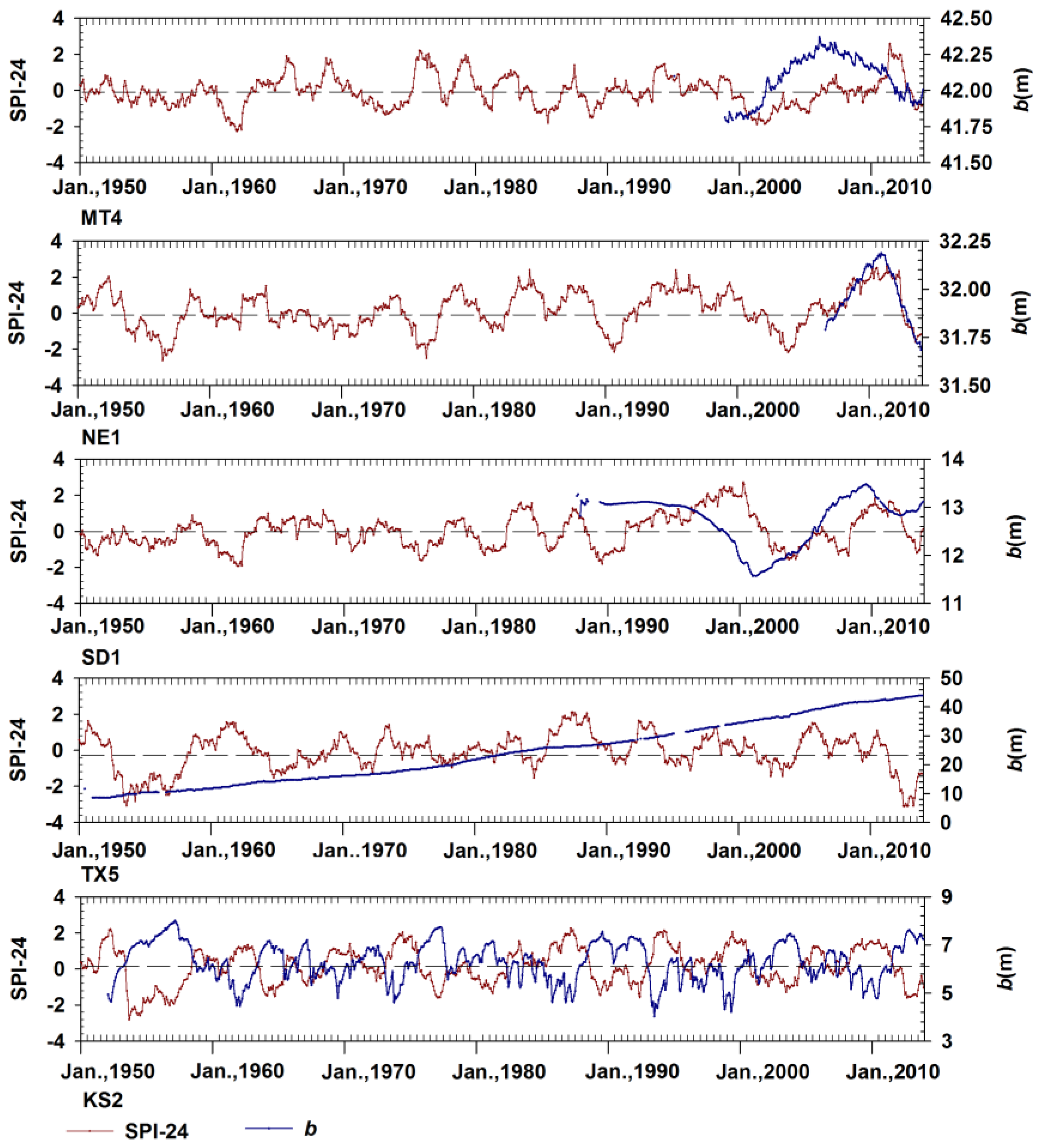
3. Results and Discussion
4. Summary and Conclusions
Acknowledgments
Author Contributions
Conflicts of Interest
Appendix A

| ID | USGS SITEID | DECLAT | DECLON | STATE | CLIM. DIVISION | COUNTY |
|---|---|---|---|---|---|---|
| CO1 | 382323104200701 | 38.390 | −104.336 | CO | ARKANSAS DRAINAGE BASIN | Pueblo |
| KS1 | 381119098435301 | 38.189 | −98.732 | KS | SOUTH CENTRAL | Stafford |
| KS2 | 390006095132301 | 39.002 | −95.223 | KS | EAST CENTRAL | Douglas |
| MT1 | 450524112380701 | 45.090 | −112.636 | MT | SOUTHWESTERN | Beaverhead |
| MT2 | 462641110561701 | 46.445 | −110.939 | MT | CENTRAL | Meagher |
| MT3 | 470709106061401 | 47.119 | −106.104 | MT | NORTHEASTERN | Garfield |
| MT4 | 472203111112602 | 47.368 | −111.191 | MT | CENTRAL | Cascade |
| MT5 | 480034105195401 | 48.009 | −105.332 | MT | NORTHEASTERN | McCone |
| ND1 | 462633097163402 | 46.442 | −97.276 | ND | SOUTHEAST | Richland |
| ND2 | 463417099271002 | 46.571 | −99.453 | ND | SOUTHEAST | Logan |
| ND3 | 465755102410701 | 46.965 | −102.686 | ND | SOUTHWEST | Stark |
| ND4 | 475646097372201 | 47.946 | −97.622 | ND | NORTHEAST | GrandForks |
| ND5 | 482908099134601 | 48.486 | −99.230 | ND | NORTHEAST | Towner |
| NE1 | 413130100531202 | 41.525 | −100.888 | NE | NORTH CENTRAL | McPherson |
| NE2 | 414607102263301 | 41.769 | −102.443 | NE | PANHANDLE | Garden |
| NE3 | 420204101200502 | 42.034 | −101.335 | NE | NORTH CENTRAL | Hooker |
| NE4 | 422802097031601 | 42.467 | −97.055 | NE | NORTHEAST | Cedar |
| NE5 | 422849099521503 | 42.480 | −99.871 | NE | NORTH CENTRAL | Brown |
| NE6 | 423148098300601 | 42.530 | −98.502 | NE | NORTH CENTRAL | Holt |
| OK1 | 343457096404501 | 34.583 | −96.679 | OK | SOUTH CENTRAL | Pontotoc |
| OK2 | 361739099323301 | 36.294 | −99.543 | OK | NORTH CENTRAL | Woodward |
| SD1 | 430027102311801 | 43.007 | −102.522 | SD | SOUTHWEST | Shannon |
| SD2 | 430027102311806 | 43.007 | −102.522 | SD | SOUTHWEST | Shannon |
| SD3 | 434330096434801 | 43.725 | −96.730 | SD | SOUTHEAST | Minnehaha |
| SD4 | 441759103261202 | 44.300 | −103.437 | SD | BLACK HILLS | Meade |
| SD5 | 442254098174501 | 44.382 | −98.296 | SD | EAST CENTRAL | Beadle |
| SD6 | 451848096363501 | 45.313 | −96.610 | SD | NORTHEAST | Grant |
| TX1 | 293202099063501 | 29.534 | −99.110 | TX | SOUTH CENTRAL | Medina |
| TX2 | 295443097554201 | 29.912 | −97.929 | TX | SOUTH CENTRAL | Hays |
| TX3 | 302948095422501 | 30.499 | −95.711 | TX | EAST TEXAS | Montgomery |
| TX4 | 303143095334801 | 30.528 | −95.564 | TX | EAST TEXAS | Walker |
| TX5 | 341010102240801 | 34.170 | −102.403 | TX | HIGH PLAINS | Lamb |
| State | Well ID | Time Span | Records (Months) | Median Depth to Water Level—Below Land Surface/(m) | |||
|---|---|---|---|---|---|---|---|
| Begin (Year/Month) | End (Year/Month) | Avg. | Max | Min | |||
| CO | CO1 | 2003/03 | 2013/12 | 130 | 6.27 | 6.53 | 6.04 |
| KS | KS1 | 2000/04 | 2013/12 | 161 | 3.45 | 5.17 | 1.14 |
| KS2 | 1952/02 | 2013/12 | 741 | 6.26 | 8.01 | 4.02 | |
| MT | MT1 | 1998/08 | 2013/12 | 183 | 49.28 | 52.19 | 44.33 |
| MT2 | 2009/01 | 2013/12 | 60 | 26.72 | 27.44 | 25.95 | |
| MT3 | 1998/04 | 2013/12 | 183 | 9.38 | 9.78 | 8.98 | |
| MT4 | 1998/12 | 2013/12 | 178 | 42.09 | 42.37 | 41.78 | |
| MT5 | 1998/10 | 2013/12 | 180 | 13.22 | 13.39 | 12.42 | |
| ND | ND1 | 1963/09 | 2013/12 | 573 | 1.65 | 2.76 | 0.42 |
| ND2 | 1978/11 | 2013/12 | 400 | 6.50 | 8.41 | 4.47 | |
| ND3 | 1968/12 | 2013/12 | 459 | 5.61 | 6.90 | 4.28 | |
| ND4 | 1968/06 | 2013/12 | 538 | 7.05 | 8.07 | 5.93 | |
| ND5 | 1980/06 | 2013/12 | 380 | 2.96 | 4.25 | 2.25 | |
| NE | NE1 | 2006/09 | 2013/12 | 88 | 31.97 | 32.19 | 31.68 |
| NE2 | 1934/08 | 2013/12 | 307 | 1.11 | 1.88 | 0.28 | |
| NE3 | 1998/12 | 2013/12 | 180 | 1.89 | 3.51 | 0.98 | |
| NE4 | 2011/10 | 2013/12 | 27 | 0.96 | 1.50 | 0.47 | |
| NE5 | 2009/10 | 2013/12 | 51 | 2.26 | 2.84 | 1.78 | |
| NE6 | 1966/10 | 2013/12 | 563 | 14.16 | 16.37 | 10.81 | |
| OK | OK1 | 1959/11 | 201312 | 637 | 33.48 | 38.96 | 22.98 |
| OK2 | 2012/07 | 201312 | 18 | 38.19 | 38.53 | 37.83 | |
| SD | SD1 | 1989/06 | 2013/12 | 294 | 12.73 | 13.48 | 11.57 |
| SD2 | 1987/10 | 2013/12 | 305 | 12.59 | 19.63 | 10.52 | |
| SD3 | 2004/02 | 2013/12 | 118 | 1.71 | 3.04 | 0.52 | |
| SD4 | 1990/11 | 2013/12 | 271 | 0.31 | 16.66 | −13.22 | |
| SD5 | 1979/06 | 2013/12 | 225 | 8.58 | 13.75 | 3.03 | |
| SD6 | 1979/10 | 2013/12 | 213 | 9.58 | 11.70 | 5.86 | |
| TX | TX1 | 2002/03 | 2013/12 | 67 | 54.19 | 58.21 | 51.42 |
| TX2 | 1980/07 | 2013/10 | 336 | 7.55 | 8.64 | 4.56 | |
| TX3 | 1952/11 | 2013/12 | 187 | 15.20 | 17.78 | 13.91 | |
| TX4 | 1989/12 | 2013/12 | 142 | 22.96 | 23.68 | 21.71 | |
| TX5 | 1951/01 | 2013/12 | 725 | 24.15 | 43.92 | 8.53 | |
References
- Leelaruban, N.; Padmanabhan, G. Droughts-groundwater relationship in Northern Great Plains Shallow Aquifers. In Proceedings of the World Environmental and Water Resources Congress, Austin, TX, USA, 17–21 May 2015; pp. 510–519. [CrossRef]
- Wilhite, D.A.; Glantz, M.H. Understanding: The drought phenomenon: The role of definitions. Water Int. 1985, 10, 111–120. [Google Scholar] [CrossRef]
- Dracup, J.A.; Lee, K.S.; Paulson, E.G. On the definition of droughts. Water Resour. Res. 1980, 16, 297–302. [Google Scholar] [CrossRef]
- Tallaksen, L.M.; Madsen, H.; Clausen, B. On the definition and modelling of streamflow drought duration and deficit volume. Hydrol. Sci. J. 1997, 42, 15–33. [Google Scholar] [CrossRef]
- Mc Kee, T.B.; Doeskin, N.J.; Kleist, J. The relationship of drought frequency and duration to time scales. In Proceedings of the 8th Conference on Applied Climatology, Anaheim, CA, USA, 17–22 January 1993; pp. 179–184.
- Steinemann, A.C.; Hayes, M.; Cavalcanti, L. Drought indicators and triggers. In Drought and Water Crises: Science, Technology, and Management Issues; Wilhite, D., Ed.; CRC Press: Boca Raton, FL, USA, 2005; pp. 71–92. [Google Scholar]
- American Meteorological Society (AMS). AMS Information Statement on Drought. 2013. Available online: https://www.ametsoc.org/ams/index.cfm/about-ams/ams-statements/statements-of-the-ams-in-force/drought/ (accessed on 25 September 2016).
- Mishra, A.K.; Singh, V.P. A review of drought concepts. J. Hydrol. 2010, 391, 204–216. [Google Scholar] [CrossRef]
- Chang, T.J.; Teoh, C.B. Use of the kriging method for studying characteristics of ground-water droughts. Water Resour. Bull. 1995, 31, 1001–1007. [Google Scholar] [CrossRef]
- Eltahir, E.A.B.; Yeh, P. On the asymmetric response of aquifer water level to floods and droughts in illinois. Water Resour. Res. 1999, 35, 1199–1217. [Google Scholar] [CrossRef]
- Van Loon, A.F. Hydrological drought explained. Wiley Interdiscip. Rev. Water 2015, 2, 359–392. [Google Scholar] [CrossRef]
- Chen, Z.H.; Grasby, S.E.; Osadetz, K.G. Predicting average annual groundwater levels from climatic variables: An empirical model. J. Hydrol. 2002, 260, 102–117. [Google Scholar] [CrossRef]
- Chen, Z.H.; Grasby, S.E.; Osadetz, K.G. Relation between climate variability and groundwater levels in the upper carbonate aquifer, Southern Manitoba, Canada. J. Hydrol. 2004, 290, 43–62. [Google Scholar] [CrossRef]
- Jan, C.D.; Chen, T.H.; Lo, W.C. Effect of rainfall intensity and distribution on groundwater level fluctuations. J. Hydrol. 2007, 332, 348–360. [Google Scholar] [CrossRef]
- Panda, D.K.; Mishra, A.; Jena, S.K.; James, B.K.; Kumar, A. The influence of drought and anthropogenic effects on groundwater levels in Orissa, India. J. Hydrol. 2007, 343, 140–153. [Google Scholar] [CrossRef]
- Tirogo, J.; Jost, A.; Biaou, A.; Valdes-Lao, D.; Koussoube, Y.; Ribstein, P. Climate variability and groundwater response: A case study in Burkina Faso (West Africa). Water 2016, 8, 171. [Google Scholar] [CrossRef]
- Mall, R.K.; Gupta, A.; Singh, R.; Singh, R.S.; Rathore, L.S. Water resources and climate change: An Indian perspective. Curr. Sci. 2006, 90, 1610–1626. [Google Scholar]
- Haslinger, K.; Koffler, D.; Schoener, W.; Laaha, G. Exploring the link between meteorological drought and streamflow: Effects of climate-catchment interaction. Water Resour. Res. 2014, 50, 2468–2487. [Google Scholar] [CrossRef]
- Vasiliades, L.; Loukas, A. Hydrological response to meteorological drought using the palmer drought indices in Thessaly, Greece. Desalination 2009, 237, 3–21. [Google Scholar] [CrossRef]
- Vicente-Serrano, S.M.; Begueria, S.; Lorenzo-Lacruz, J.; Julio Camarero, J.; Lopez-Moreno, J.I.; Azorin-Molina, C.; Revuelto, J.; Moran-Tejeda, E.; Sanchez-Lorenzo, A. Performance of drought indices for ecological, agricultural, and hydrological applications. Earth Interact. 2012, 16, 1–27. [Google Scholar] [CrossRef]
- Lorenzo-Lacruz, J.; Vicente-Serrano, S.M.; Lopez-Moreno, J.I.; Begueria, S.; Garcia-Ruiz, J.M.; Cuadrat, J.M. The impact of droughts and water management on various hydrological systems in the headwaters of the Tagus river (central Spain). J. Hydrol. 2010, 386, 13–26. [Google Scholar] [CrossRef] [Green Version]
- Shahid, S.; Hazarika, M.K. Groundwater drought in the northwestern districts of Bangladesh. Water Resour. Manag. 2010, 24, 1989–2006. [Google Scholar] [CrossRef]
- Fiorillo, F.; Guadagno, F.M. Long karst spring discharge time series and droughts occurrence in Southern Italy. Environ. Earth Sci. 2012, 65, 2273–2283. [Google Scholar] [CrossRef]
- Bloomfield, J.P.; Marchant, B.P. Analysis of groundwater drought building on the standardised precipitation index approach. Hydrol. Earth Syst. Sci. 2013, 17, 4769–4787. [Google Scholar] [CrossRef] [Green Version]
- Mendicino, G.; Senatore, A.; Versace, P. A groundwater resource index (GRI) for drought monitoring and forecasting in a mediterranean climate. J. Hydrol. 2008, 357, 282–302. [Google Scholar] [CrossRef]
- Li, B.; Rodell, M. Evaluation of a model-based groundwater drought indicator in the conterminous U.S. J. Hydrol. 2014, 526, 78–88. [Google Scholar] [CrossRef]
- Koster, R.D.; Suarez, M.J.; Ducharne, A.; Stieglitz, M.; Kumar, P. A catchment-based approach to modeling land surface processes in a general circulation model 1. Model structure. J. Geophys. Res. Atmos. 2000, 105, 24809–24822. [Google Scholar] [CrossRef]
- Jaranilla-Sanchez, P.A.; Wang, L.; Koike, T. Modeling the hydrologic responses of the Pampanga River basin, Philippines: A quantitative approach for identifying droughts. Water Resour. Res. 2011, 47. [Google Scholar] [CrossRef]
- Sawada, Y.; Koike, T.; Jaranilla-Sanchez, P.A. Modeling hydrologic and ecologic responses using a new eco-hydrological model for identification of droughts. Water Resour. Res. 2014, 50, 6214–6235. [Google Scholar] [CrossRef]
- Rodell, M.; Velicogna, I.; Famiglietti, J.S. Satellite-based estimates of groundwater depletion in India. Nature 2009, 460, 999–1002. [Google Scholar] [CrossRef] [PubMed]
- Famiglietti, J.S.; Lo, M.; Ho, S.L.; Bethune, J.; Anderson, K.J.; Syed, T.H.; Swenson, S.C.; de Linage, C.R.; Rodell, M. Satellites measure recent rates of groundwater depletion in California’s central valley. Geophys. Res. Lett. 2011, 38, L03403. [Google Scholar] [CrossRef]
- Voss, K.A.; Famiglietti, J.S.; Lo, M.; de Linage, C.; Rodell, M.; Swenson, S.C. Groundwater depletion in the middle east from grace with implications for transboundary water management in the Tigris-Euphrates-Western Iran region. Water Resour. Res. 2013, 49, 904–914. [Google Scholar] [CrossRef] [PubMed]
- Castle, S.L.; Thomas, B.F.; Reager, J.T.; Rodell, M.; Swenson, S.C.; Famiglietti, J.S. Groundwater depletion during drought threatens future water security of the Colorado River basin. Geophys. Res. Lett. 2014, 41, 5904–5911. [Google Scholar] [CrossRef] [PubMed]
- Whittemore, D.O.; Butler, J.J.; Wilson, B.B. Assessing the major drivers of water-level declines: New insights into the future of heavily stressed aquifers. Hydrol. Sci. J. 2016, 61, 134–145. [Google Scholar] [CrossRef]
- Cunningham, W.L.; Geiger, L.H.; Karavitis, G.A. U.S. Geological Survey Ground-Water Climate Response Network. U.S. Geological Survey Fact Sheet 2007–3003; 2007; 4p. Available online: http://pubs.usgs.gov/fs/2007/3003/ (accessed on 25 September 2016). [Google Scholar]
- Palmer, W.C. Meteorological Drought; Research Paper No. 45; U.S. Department of Commerce, Weather Bureau: Washington, DC, USA, 1965; p. 58.
- Karl, T.R. The sensitivity of the palmer drought severity index and palmer z-index to their calibration coefficients including potential evapotranspiration. J. Clim. Appl. Meteorol. 1986, 25, 77–86. [Google Scholar] [CrossRef]
- Mc Kee, T.B.; Doeskin, N.J.; Kleist, J. Drought Monitoring with Multiple Time Scales. In Proceedings of the 9th Conference on Applied Climatology, Dallas, TX, USA, 15–20 January 1995; pp. 233–236.
- Fenimore, C.; Arndt, D.; Gleason, K.; Heim, R.R., Jr. Transitioning from the traditional divisional dataset to the Global Historical Climatology Network-Daily gridded divisional dataset. In Proceedings of the 23rd Conference on Climate Variability and Change, Seattle, WA, USA, 22–27 January 2011; Paper Number 6B.5. Available online: https://www.ncdc.noaa.gov/monitoring-references/docs/GrDD-Transition.pdf (accessed on 25 September 2016).
- Vose, R.S.; Applequist, S.; Squires, M.; Durre, I.; Menne, M.J.; Williams, C.N., Jr.; Fenimore, C.; Gleason, K.; Arndt, D. Improved historical temperature and precipitation time series for U.S. climate divisions. J. Appl. Meteorol. Climatol. 2014, 53, 1232–1251. [Google Scholar] [CrossRef]
- Svoboda, M.; Hayes, M.; Wood, D. Standardized Precipitation Index User Guide; Technical Report WMO-No. 1090; World Meteorological Organization: Geneva, Switzerland, 2012; Available online: http://www.wamis.org/agm/pubs/SPI/WMO_1090_EN.pdf (accessed on 25 September 2016).
- Guttman, N.B.; Quayle, R.G. A historical perspective of U.S. climate divisions. Bull. Am. Meteorol. Soc. 1996, 77, 293–303. [Google Scholar] [CrossRef]
- Karl, T.; Koss, W.J. Regional and National Monthly, Seasonal, and Annual Temperature Weighted by Area, 1895–1983; Technical Report; Volume 4, Issue 3 of Historical Climatology Series; National Climatic Data Center: Asheville, NC, USA, 1984; 38p. [Google Scholar]
- Hayes, M.; Svoboda, M.; Wall, N.; Widhalm, M. The lincoln declaration on drought indices. Bull. Am. Meteorol. Soc. 2011, 92, 485–488. [Google Scholar] [CrossRef]


| Well ID | Coef. | SE | T | P | Well ID | Coef. | SE | T | P | ||
|---|---|---|---|---|---|---|---|---|---|---|---|
| CO1 | β0 | 6.25 | 0.01 | 602.78 | 0.000 | NE4 | β0 | 0.78 | 0.04 | 17.38 | 0.000 |
| β1 | −0.04 | 0.01 | −4.89 | 0.000 | β1 | −0.25 | 0.03 | −7.28 | 0.000 | ||
| KS1 | β0 | 3.79 | 0.07 | 57.26 | 0.000 | NE5 | β0 | 2.44 | 0.03 | 75.56 | 0.000 |
| β1 | −0.70 | 0.06 | −11.57 | 0.000 | β1 | −0.17 | 0.02 | −9.52 | 0.000 | ||
| KS2 | β0 | 6.35 | 0.02 | 360.74 | 0.000 | NE6 | β0 | 14.18 | 0.05 | 258.48 | 0.000 |
| β1 | −0.60 | 0.02 | −35.28 | 0.000 | β1 | −0.05 | 0.05 | −1.08 | 0.280 | ||
| MT1 | β0 | 48.72 | 0.14 | 347.19 | 0.000 | OK1 | β0 | 33.77 | 0.08 | 438.32 | 0.000 |
| β1 | −1.28 | 0.14 | −8.88 | 0.000 | β1 | −1.76 | 0.08 | −22.91 | 0.000 | ||
| MT2 | β0 | 26.83 | 0.05 | 577.91 | 0.000 | OK2 | β0 | 38.07 | 0.09 | 404.35 | 0.000 |
| β1 | −0.26 | 0.04 | −5.85 | 0.000 | β1 | −0.13 | 0.09 | −1.49 | 0.156 | ||
| MT3 | β0 | 9.40 | 0.01 | 761.55 | 0.000 | SD1 | β0 | 12.72 | 0.03 | 403.61 | 0.000 |
| β1 | −0.05 | 0.01 | −4.37 | 0.000 | β1 | 0.02 | 0.03 | 0.73 | 0.464 | ||
| MT4 | β0 | 42.09 | 0.01 | 3363.45 | 0.000 | SD2 | β0 | 12.70 | 0.11 | 120.18 | 0.000 |
| β1 | 0.03 | 0.01 | 2.09 | 0.038 | β1 | −0.35 | 0.09 | −3.71 | 0.000 | ||
| MT5 | β0 | 13.30 | 0.01 | 1123.18 | 0.000 | SD3 | β0 | 2.07 | 0.06 | 36.90 | 0.000 |
| β1 | −0.16 | 0.01 | −14.37 | 0.000 | β1 | −0.45 | 0.05 | −9.94 | 0.000 | ||
| ND1 | β0 | 1.72 | 0.02 | 83.83 | 0.000 | SD4 | β0 | 2.00 | 0.42 | 4.73 | 0.000 |
| β1 | −0.35 | 0.02 | −17.33 | 0.000 | β1 | −5.21 | 0.40 | −13.00 | 0.000 | ||
| ND2 | β0 | 6.60 | 0.04 | 161.51 | 0.000 | SD5 | β0 | 9.09 | 0.18 | 49.28 | 0.000 |
| β1 | −0.24 | 0.04 | −6.62 | 0.000 | β1 | −1.32 | 0.19 | −7.07 | 0.000 | ||
| ND3 | β0 | 5.64 | 0.02 | 348.93 | 0.000 | SD6 | β0 | 9.68 | 0.09 | 110.93 | 0.000 |
| β1 | −0.27 | 0.02 | −16.58 | 0.000 | β1 | −0.89 | 0.10 | −9.23 | 0.000 | ||
| ND4 | β0 | 7.12 | 0.02 | 378.18 | 0.000 | TX1 | β0 | 54.16 | 0.14 | 377.00 | 0.000 |
| β1 | −0.22 | 0.02 | −11.58 | 0.000 | β1 | 0.08 | 0.13 | 0.58 | 0.565 | ||
| ND5 | β0 | 3.10 | 0.02 | 160.01 | 0.000 | TX2 | β0 | 7.66 | 0.04 | 196.64 | 0.000 |
| β1 | −0.29 | 0.02 | −16.72 | 0.000 | β1 | −0.44 | 0.04 | −11.38 | 0.000 | ||
| NE1 | β0 | 31.87 | 0.01 | 4149.44 | 0.000 | TX3 | β0 | 15.21 | 0.03 | 436.75 | 0.000 |
| β1 | 0.11 | 0.00 | 21.23 | 0.000 | β1 | −0.09 | 0.03 | −2.76 | 0.006 | ||
| NE2 | β0 | 1.09 | 0.01 | 78.48 | 0.000 | TX4 | β0 | 22.99 | 0.03 | 886.17 | 0.000 |
| β1 | −0.17 | 0.01 | −13.75 | 0.000 | β1 | −0.15 | 0.02 | −6.59 | 0.000 | ||
| NE3 | β0 | 1.93 | 0.04 | 45.52 | 0.000 | TX5 | β0 | 24.23 | 0.40 | 60.91 | 0.000 |
| β1 | −0.09 | 0.03 | −2.69 | 0.008 | β1 | 0.94 | 0.40 | 2.35 | 0.019 |
| ID (Time Frame) | Pr | January | February | March | April | May | June | July | August | September | October | November | December |
|---|---|---|---|---|---|---|---|---|---|---|---|---|---|
| KS2 (1953–2013) | r′ | −0.84 | −0.82 | −0.82 | −0.78 | −0.81 | −0.79 | −0.77 | −0.76 | −0.75 | −0.80 | −0.81 | −0.82 |
| n | 61 | 60 | 61 | 61 | 61 | 61 | 61 | 61 | 61 | 61 | 61 | 60 | |
| μ | 6.38 | 6.39 | 6.34 | 6.24 | 6.14 | 6.03 | 6.12 | 6.31 | 6.38 | 6.32 | 6.32 | 6.35 | |
| ND1 (1964–2013) | r′ | −0.75 | −0.72 | −0.73 | −0.60 | −0.57 | −0.57 | −0.60 | −0.65 | −0.67 | −0.68 | −0.69 | −0.69 |
| n | 49 | 44 | 48 | 49 | 46 | 47 | 47 | 47 | 47 | 48 | 48 | 49 | |
| μ | 1.92 | 1.97 | 1.83 | 1.21 | 1.18 | 1.31 | 1.48 | 1.79 | 1.87 | 1.77 | 1.67 | 1.77 | |
| ND2 (1979–2013) | r′ | −0.42 | −0.38 | −0.31 | −0.36 | −0.30 | −0.33 | −0.32 | −0.31 | −0.29 | −0.29 | −0.24 | −0.28 |
| n | 29 | 28 | 33 | 33 | 35 | 35 | 35 | 35 | 34 | 35 | 35 | 32 | |
| μ | 6.52 | 6.52 | 6.48 | 6.41 | 6.36 | 6.36 | 6.47 | 6.65 | 6.69 | 6.58 | 6.50 | 6.51 | |
| ND3 (1969–2013) | r′ | −0.68 | −0.68 | −0.67 | −0.60 | −0.73 | −0.64 | −0.55 | −0.58 | −0.65 | −0.66 | −0.67 | −0.72 |
| n | 36 | 37 | 39 | 36 | 32 | 42 | 39 | 41 | 36 | 44 | 40 | 36 | |
| μ | 5.77 | 5.76 | 5.64 | 5.45 | 5.45 | 5.40 | 5.47 | 5.58 | 5.68 | 5.66 | 5.67 | 5.73 | |
| ND4 (1966–2013) | r′ | −0.43 | −0.34 | −0.34 | −0.38 | −0.36 | −0.48 | −0.43 | −0.35 | −0.36 | −0.38 | −0.37 | −0.41 |
| n | 45 | 45 | 47 | 46 | 46 | 46 | 45 | 46 | 47 | 46 | 47 | 47 | |
| μ | 7.07 | 7.08 | 7.11 | 7.06 | 7.03 | 7.00 | 7.03 | 7.11 | 7.14 | 7.09 | 7.08 | 7.07 | |
| ND5 (1981–2013) | r′ | −0.68 | −0.68 | −0.67 | −0.64 | −0.68 | −0.73 | −0.58 | −0.64 | −0.63 | −0.61 | −0.62 | −0.65 |
| n | 31 | 29 | 29 | 31 | 33 | 33 | 30 | 31 | 30 | 33 | 32 | 31 | |
| μ | 2.96 | 3.01 | 3.04 | 3.03 | 3.03 | 2.95 | 2.90 | 2.85 | 2.93 | 2.93 | 2.93 | 2.93 | |
| NE6 (1967–2013) | r′ | −0.04 | −0.06 | −0.06 | −0.07 | −0.08 | −0.02 | −0.04 | −0.02 | −0.02 | −0.01 | −0.04 | −0.05 |
| n | 46 | 46 | 47 | 47 | 47 | 47 | 46 | 46 | 47 | 47 | 47 | 47 | |
| μ | 14.18 | 14.17 | 14.11 | 14.06 | 14.01 | 13.98 | 14.02 | 14.24 | 14.35 | 14.37 | 14.35 | 14.33 | |
| OK1 (1960–2013) | r′ | −0.75 | −0.71 | −0.73 | −0.62 | −0.73 | −0.76 | −0.71 | −0.69 | −0.75 | −0.75 | −0.71 | −0.70 |
| n | 52 | 52 | 52 | 54 | 52 | 53 | 54 | 52 | 53 | 54 | 53 | 54 | |
| μ | 33.71 | 33.75 | 33.42 | 32.66 | 32.27 | 32.14 | 32.79 | 33.80 | 34.44 | 34.49 | 34.20 | 34.02 | |
| TX2 (1981–2013) | r′ | −0.52 | −0.54 | −0.50 | −0.48 | −0.59 | −0.62 | −0.53 | −0.52 | −0.55 | −0.62 | −0.59 | −0.55 |
| n | 28 | 25 | 30 | 28 | 27 | 27 | 29 | 27 | 28 | 28 | 27 | 26 | |
| μ | 7.44 | 7.44 | 7.56 | 7.56 | 7.59 | 7.37 | 7.40 | 7.59 | 7.69 | 7.74 | 7.59 | 7.48 |
| ID | Drought Events | |||
|---|---|---|---|---|
| Start | End | Duration (Months) | # Records | |
| KS2 | July 1953 | October 1957 | 52 | 52 |
| MT1 | June 2000 | April 2003 | 35 | 35 |
| MT4 | June 2000 | February 2003 | 33 | 32 |
| ND3 | May 1989 | July 1992 | 39 | 39 |
| ND4 | July 1988 | June 1991 | 36 | 36 |
| ND5 | July 1988 | June 1991 | 36 | 35 |
| NE2 | August 1935 | August 1938 | 37 | 30 |
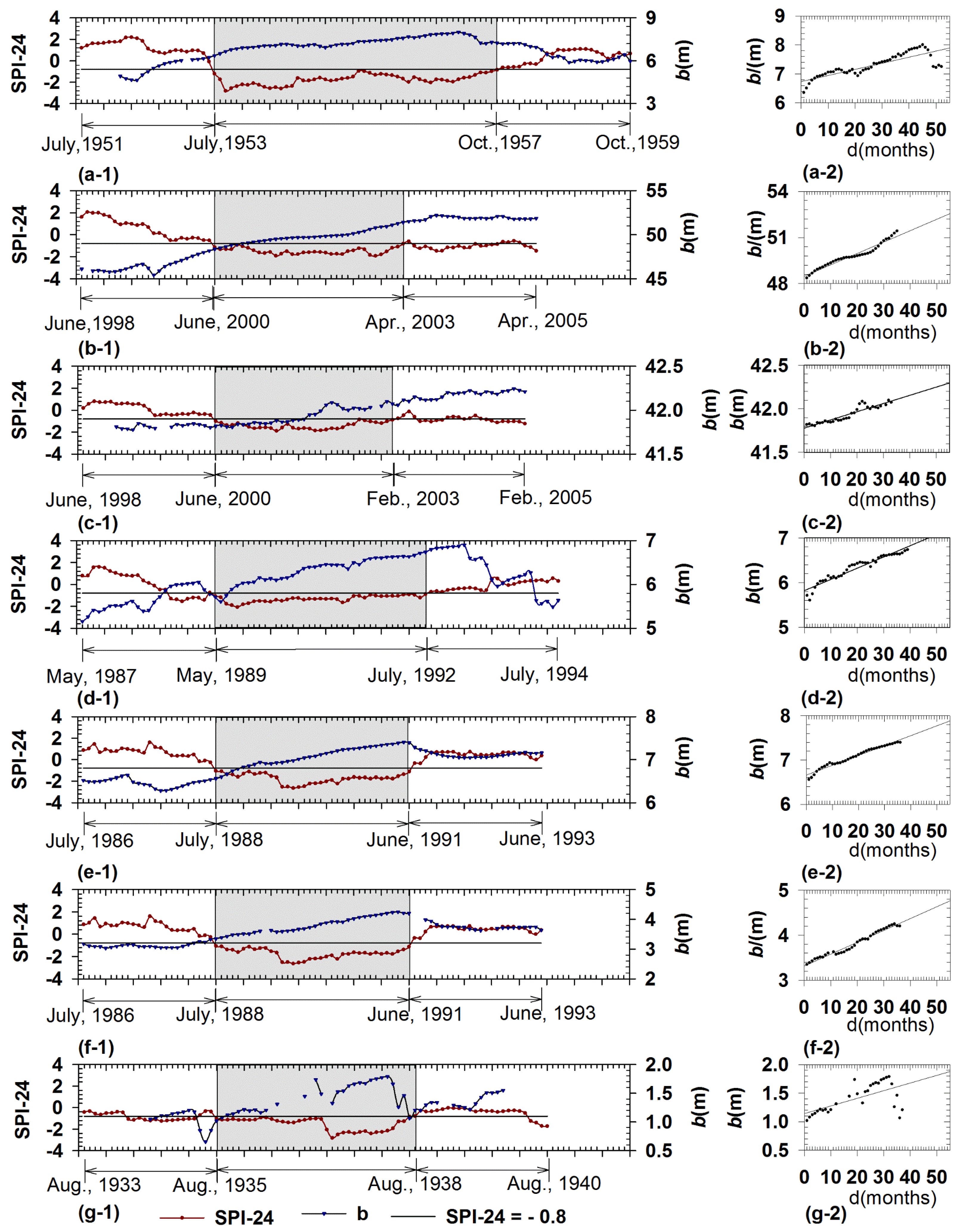
| ID | Time Frame | Total Drop (m) | r | Regression Model | R2 (%) | |
|---|---|---|---|---|---|---|
| Start | End | |||||
| KS2 | July 1953 | October 1957 | 0.90 | 0.831 | b = 0.021d + 6.734 | 69.1 |
| MT1 | June 2000 | April 2003 | 3.05 | 0.976 | b = 0.074d + 48.478 | 95.3 |
| MT4 | June 2000 | February 2003 | 0.25 | 0.933 | b = 0.009d + 41.779 | 87.1 |
| ND3 | May 1989 | July 1992 | 1.02 | 0.962 | b = 0.025d + 5.825 | 92.5 |
| ND4 | July 1988 | June 1991 | 0.84 | 0.986 | b = 0.022d + 6.653 | 97.3 |
| ND5 | July 1988 | June 1991 | 0.85 | 0.987 | b = 0.026d + 3.318 | 97.4 |
| NE2 | August 1935 | August 1938 | 0.19 | 0.625 | b = 0.013d + 1.143 | 39.0 |
© 2017 by the authors. Licensee MDPI, Basel, Switzerland. This article is an open access article distributed under the terms and conditions of the Creative Commons Attribution (CC BY) license ( http://creativecommons.org/licenses/by/4.0/).
Share and Cite
Leelaruban, N.; Padmanabhan, G.; Oduor, P. Examining the Relationship between Drought Indices and Groundwater Levels. Water 2017, 9, 82. https://doi.org/10.3390/w9020082
Leelaruban N, Padmanabhan G, Oduor P. Examining the Relationship between Drought Indices and Groundwater Levels. Water. 2017; 9(2):82. https://doi.org/10.3390/w9020082
Chicago/Turabian StyleLeelaruban, Navaratnam, G. Padmanabhan, and Peter Oduor. 2017. "Examining the Relationship between Drought Indices and Groundwater Levels" Water 9, no. 2: 82. https://doi.org/10.3390/w9020082