Article

Effective Saturated Hydraulic Conductivity for Representing Field-Scale Infiltration and Surface Soil Moisture in Heterogeneous Unsaturated Soils Subjected to Rainfall Events

1
Indian Institute of Technology, Kanpur 208016, India
2
Department of Civil and Environmental Engineering, University of Perugia, via G. Duranti 93, 06125 Perugia, Italy
3
Lyles School of Civil Engineering, Purdue University, West Lafayette, IN 47907, USA
*
Author to whom correspondence should be addressed.
Water 2017, 9(2), 134; https://doi.org/10.3390/w9020134
Submission received: 16 December 2016 / Revised: 9 February 2017 / Accepted: 13 February 2017 / Published: 20 February 2017

Abstract

:
Spatial heterogeneity in soil properties has been a challenge for providing field-scale estimates of infiltration rates and surface soil moisture content over natural fields. In this study, we develop analytical expressions for effective saturated hydraulic conductivity for use with the Green-Ampt model to describe field-scale infiltration rates and evolution of surface soil moisture over unsaturated fields subjected to a rainfall event. The heterogeneity in soil properties is described by a log-normal distribution for surface saturated hydraulic conductivity. Comparisons between field-scale numerical and analytical simulation results for water movement in heterogeneous unsaturated soils show that the proposed expressions reproduce the evolution of surface soil moisture and infiltration rate with time. The analytical expressions hold promise for describing mean field infiltration rates and surface soil moisture evolution at field-scale over sandy loam and loamy sand soils.

1. Introduction

Determination of infiltration rates and surface soil moisture variation at a range of scales is useful in hydrologic and climatic modeling, and prediction studies [1,2]. The Richards equation is a physically-based model that is utilized to discern infiltration rates and soil moisture variation in unsaturated soils at field-scale. This equation is highly non-linear and imposes a heavy computational burden, especially when describing water movement in initially dry soils [3]. Moreover, detailed data on soil properties in the study area are needed for implementing the Richards equation at its full potential. Such data are rarely available, and studies often resort to calibration exercises to estimate unknown quantities.
The description of infiltration rates and surface soil moisture at different spatial and temporal scales is complicated further by the spatial heterogeneity exhibited by the hydraulic properties of the field-soils [4,5,6]. To estimate the spatial and temporal variation of surface soil moisture content and infiltration rates, ground-based measurements are most commonly used. These measurements provide information on soil moisture data and infiltration rates at a local-scale [7], even though conflicting results from in situ-measurements of saturated hydraulic conductivity by different devices have been obtained. Moreover, the measurements are expensive, time consuming, provide data at few selected points, and require accurate calibration of the measuring instrument. Further, reliable interpretation of spatial and temporal patterns of infiltration rates and surface soil moisture at different scales from measurements available at few selected points is very challenging [8].
An alternate approach for predicting mean flow behavior at the field-scale has been upscaling i.e., to represent the heterogeneous domain by an equivalent homogeneous domain with upscaled (effective or macroscopic) flow properties [9,10]. The upscaling procedures presently available can be broadly categorized as (1) forward upscaling and (2) inverse upscaling.
Forward upscaling relies on deriving the effective parameters and upscaled flow equations by considering information about the spatial structure and variability of soil hydraulic properties measured at the local-scale [10,11]. Stochastic perturbation-based methods [12,13,14,15,16] and stochastic streamtube-based approaches [17,18,19,20,21] have been widely popular in this regard. Perturbation-based methods are constrained to cases of small variations in soil properties, and the resulting equations for effective soil hydraulic parameters and field-scale flow are computationally intensive because of high dimensionality, intercoupling, and nonlinearity [10]. Stochastic streamtube models are better suited for highly heterogeneous soils. However, obtaining field-scale solutions from a local-scale solution in a stochastic streamtube framework often requires computationally intensive Monte-Carlo simulations [22].
Inverse scaling methods utilize information about the measurement and observations of spatial variability of soil properties, state variables of soil water processes (e.g., soil moisture content, or soil water tension) and boundary fluxes at various scales to derive effective parameters of the heterogeneous system at a large scale [9,10]. These methods mainly assume that the effective flow equations are known a-priori at the large-scale. Few studies have also derived field-scale effective properties using inverse scaling methods [23,24,25]. Yeh et al. [25] and Ye et al. [24] used spatial moment analysis to derive expressions for three-dimensional effective unsaturated hydraulic conductivity tensor from soil moisture observations under transient flow-conditions. Ward et al. [23] applied effective medium approximation method to estimate upscaled water retention characteristics and effective unsaturated hydraulic conductivity from the observed moisture distribution for a field-scale water injection test. The proposed inverse scaling methods for estimating effective parameters at field-scale require extensive soil moisture measurements and are suited for low values of soil moisture.
Many watershed models, e.g., SWAT [26], GSSHA [27], and KINEROS2 [28] partition the study area into smaller “field-scale” units and assume homogeneous properties within each unit. When using such models, a fundamental question of incorporating the effects of subgrid heterogeneity needs to be addressed. A viable approach is to replace the heterogeneous soil system with equivalent soil properties so that a deterministic homogeneous solution mimics field-scale behavior with sufficient accuracy. Since a straightforward statistical average does not meet this need when the governing processes and transformations are nonlinear, procedures for estimation of effective saturated soil hydraulic conductivity in such contexts is useful, and is the subject of this paper.
Additionally, it is noteworthy that most of the field-scale studies have focused on estimating analytical expressions for effective soil hydraulic parameters for steady or gravity dominated flow conditions [29]. However, for field conditions where the soil is subjected to rainfall or irrigation events, the boundary conditions change from being rainfall-controlled to soil-controlled in different parts of the field, and transient flow conditions are arguably just as prevalent [30]. Obtaining analytical expressions for effective soil hydraulic properties at field-scale for non-linear Richards equation under such a boundary condition is more complex, and has not received enough attention in the literature. The KINEROS2 model does have a feature for representing the spatial variability of K s , but this feature needs to be tested.
As upscaling of Richards equation under such dynamic boundary conditions is complex, approximate local models are sought for enabling mathematically-tractable field-scale solutions [31]. When seeking field-scale solutions, researchers note that errors incurred by using simplified local models tend to cancel out due to large-scale variability in soil parameters [17,18,32,33,34]. Under this hypothesis, the evolution of surface soil moisture and infiltration rates at a local-scale under a single rainfall event are described using a sharp front model for water movement. Subsequently, utilizing the field-scale spatial variability in saturated hydraulic conductivity, analytical solutions for effective saturated hydraulic conductivity are developed.
We assume that the 3-D soil field is represented as a collection of independent streamtubes with only vertical flow, and the saturated hydraulic conductivity, K s , follows a lognormal distribution over the field. Other soil parameters of Brooks and Corey model, λ , θ s , θ i , ψ b (see below Equation (2)) are considered as constants. The streamtube model is a good approximation at shallow depth under high recharge rates, and when the horizontal correlation length scale is much larger than the vertical length scale [17,18,20,31,35,36,37,38]. The surface saturated hydraulic conductivity has been found to exhibit a variation that is typically represented by a lognormal distribution, e.g., [17,18,22,35]. Specifically, Russo and Bresler [39] found that the variation in parameters, λ , θ s , θ i , ψ b , to be smaller than that associated with K s , a fact that is supported by experimental studies as well, e.g., [40,41].
The primary goal of the study is to develop analytical expressions for effective saturated hydraulic conductivity to describe the temporal evolution of surface soil moisture and infiltration rates under a rainfall event. These expressions can be used to mimic field-scale variability in current watershed models (such as SWAT, KINEROS, GSSHA and others) that utilize the Green-Ampt method to describe infiltration rate in homogeneous soils. First, local-scale models of infiltration rate and soil moisture are described from a sharp-front model for water movement. Then, assuming a lognormally distributed horizontal random field for saturated hydraulic conductivity, analytical expressions for the effective saturated hydraulic conductivity are developed. Comparisons of the results obtained from this model with extensive sets of Monte Carlo simulations, 3-D numerical solutions and field-scale analytical results are performed to evaluate the applicability of the expressions for effective hydraulic conductivity.

2. Materials and Methods

The governing differential equations and notation in this section are similar to those of previous studies [30,31]. The one-dimensional vertical Richards equation for water movement in unsaturated soils is,
θ t z [ K ( ψ ) ( ψ z 1 ) ] = 0
where θ is the volumetric water content, t is time and z is the vertical coordinate pointing downwards. The Brooks and Corey model [42] is often used to describe unsaturated soil properties in Equation (1). The soil-water saturation, pressure head, and conductivity are related as,
K r ( ψ ) = K ( ψ ) K s = ( ψ b ψ ) n ; S = θ θ r θ s θ r = ( ψ b ψ ) λ ψ > ψ b ;   n = 2 + 3 λ
where the conductivity K ( ψ ) depends on the capillary pressure head, ψ , saturated hydraulic conductivity, K s , air entry capillary pressure head, ψ b , and the pore size distribution index, λ . Here θ s and θ r represent the saturated and residual water contents, respectively. Note that the present analysis is only applicable when the soil characteristic curves are described by the Brooks and Corey model.
Under the sharp-front model for water movement, the cumulative infiltrated depth of water into the soil for constant rainfall rate r is [43],
F = r t , t t p F = F p + Δ ψ Δ θ ln ( Δ ψ Δ θ + F Δ ψ Δ θ + F p ) + K s ( t t p ) , t > t p
In Equation (3), Δ ψ is the capillary pressure head difference between the soil surface and the front, and can be computed as Δ ψ = ψ b / ( 1 η ) [18], and Δ θ = ( θ s θ i ) is the difference between the water content at saturation and the initial water content. The subscript p refers to conditions at ponding. The ponding time t p and cumulative infiltrated depth of water at ponding are given by
F p = K s Δ ψ Δ θ r K s ; t p = F p r r > K s
The following dimensionless variables are defined.
θ t = θ t θ i θ s θ i ; t = t r Δ ψ Δ θ ; y = K s r ; F = F Δ ψ Δ θ ; t p = t p r Δ ψ Δ θ = y 1 y F p = F p Δ ψ Δ θ = y 1 y
where, θ t is the surface soil moisture at any time t .

Field-Scale Solution

At the field scale, the quantity y is assumed to vary spatially following a log-normal distribution with the density function.
f y ( y ; μ Y , σ Y ) = 1 2 π σ Y y exp [ ( ln y μ Y ) 2 2 σ Y 2 ]
where, μ Y and σ Y are the mean and standard deviation of Y = ln y = ln ( K s / r ) .
The truncated moments of the log-normal distribution are [4]:
G Y ( y c , ζ ) = 0 y c y ζ f y ( y ) d y = exp ( ζ μ Y + σ Y 2 ζ 2 2 ) [ 1 1 2 e r f c ( ln y c μ Y 2 σ Y σ Y ζ 2 ) ]
where e r f c ( ) is the complimentary error function.

Effective Value for Replicating Field-Scale Infiltration Rates

Often, field-scale rainfall and runoff data are available from which field-scale infiltration rates can be computed. The problem of estimating the effective value of K s that will honor these observations is challenging because local-scale infiltration, I is known to be highly nonlinear, with infiltration rates governed by rainfall rate until ponding time, and then controlled by soil properties. When developing an expression for effective saturated hydraulic conductivity K s (or y), we are governed by preserving the correct limiting properties so that the infiltration rates obtained from effective properties using the deterministic Green-Ampt model replicate field-scale infiltration rates at small and large times. By utilizing the theories developed in earlier studies of Govindaraju et al. [4] the following expression for effective value of y e f f is proposed to incorporate spatial variability of soil hydraulic properties for predicting infiltrations rates at the field-scale.
y e f f = K s e f f r = [ 1 G Y ( 1 , 0 ) ] + G Y ( 1 , 1 )

Effective Value for Replicating Surface Soil Moisture

Because the Green-Ampt equation is an approximate form of the Richards equation, the effective value of y in Equation (8), while suitable for field-scale infiltration rates, does not replicate field-scale surface soil moisture well, and a different tack has to be employed. The expression for effective saturated hydraulic conductivity that can describe mean field-scale surface soil moisture evolution for any duration of rainfall t r , and t r = t r r Δ ψ Δ θ is obtained by equating the water content values at local and field-scale at the cessation of rainfall. Thus, the evolution of soil moisture at local-scale just prior to cessation of rain ( t = t r ) can be expressed as,
θ t r = { 1 y e f f [ t r t r + 1 ] } 2 λ / ( 7 λ + 3 )
The mean-field soil moisture content just prior to cessation of rain ( t = t r ) can be evaluated (see Appendix A.1.2) as,
E [ θ t r ] = ( t r t r + 1 ) 2 λ / ( 7 λ + 3 ) [ G ( , 2 λ 7 λ + 3 ) G ( K c r , 2 λ 7 λ + 3 ) ] + G ( K c r , 0 )
where K c r = t r 1 + t r By setting θ t r = E [ θ t r ] in Equations (10) and (11), we obtain y e f f as,
y e f f = [ G ( , 2 λ 7 λ + 3 ) G ( K c r , 2 λ 7 λ + 3 ) + G ( K c r , 0 ) ( t r t r + 1 ) 2 λ / ( 7 λ + 3 ) ] ( ( 7 λ + 3 ) / 2 λ )
This value of y e f f holds for t > t r as well and is more suited for initially dry sandy loam soils ( θ i θ r 0 ; λ 1 ) .

3. Design of Numerical Schemes

The analytical expressions for y e f f developed in this study were used in the approximate 1-D analytical Green-Ampt model and 1-D Richards equation for field-scale surface soil moisture and infiltration rates. For comparison the following numerical schemes were also utilized:
(a)
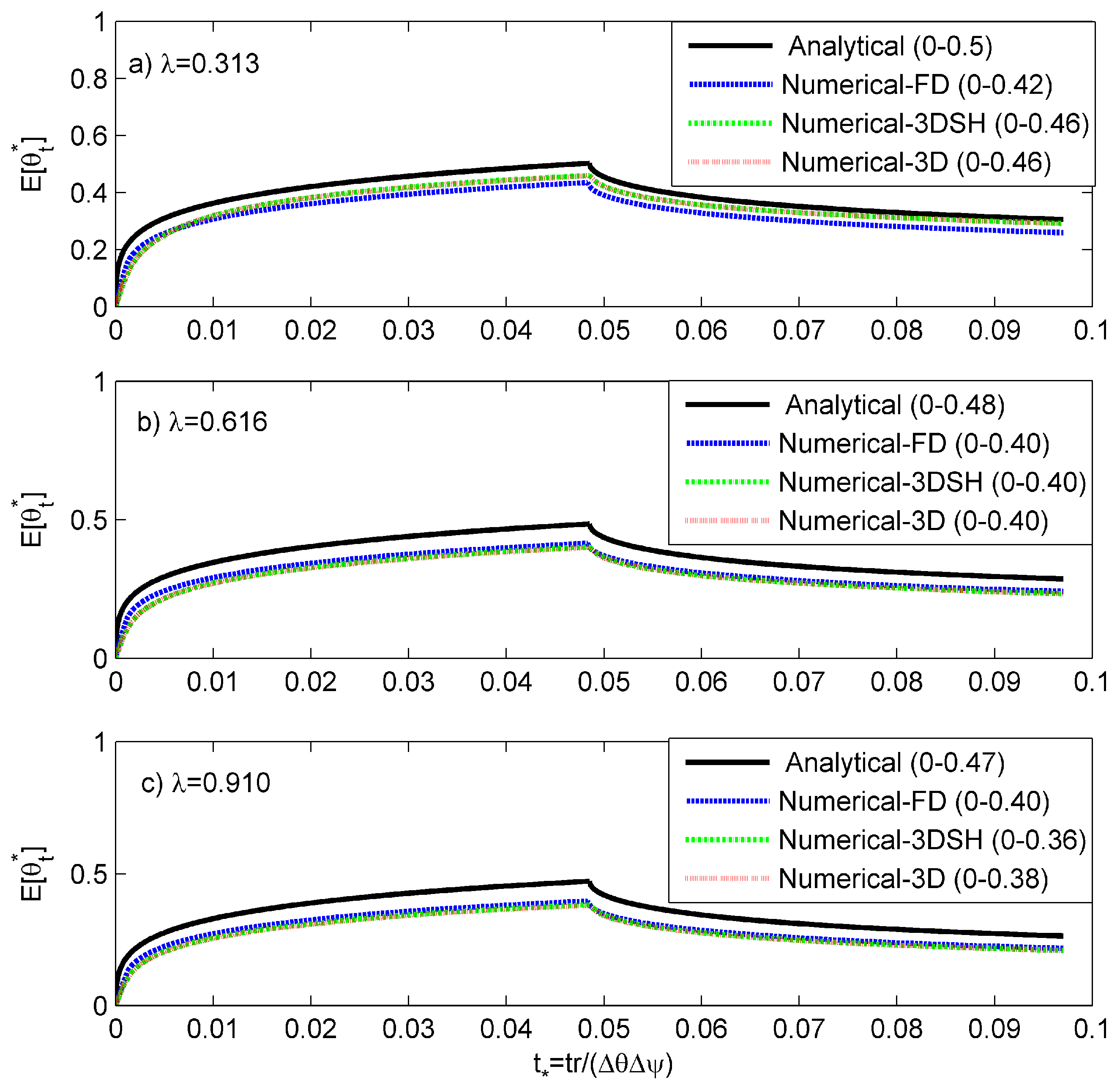
Numerical-FD: A numerical scheme denoted as “Numerical-FD” was implemented for Monte-Carlo simulations. In this scheme, from a prescribed lognormal distribution, a random value of K s was drawn. Further, the numerical solution of the Richards equation (Equations (1)–(3)) was obtained using an implicit finite difference scheme. The water content, θ ( z , t ) , fields so generated were stored for this single realization of K s , and 2000 such Monte Carlo simulations were utilized to obtain the field-scale surface soil moisture, E [ θ t ] and infiltration rates, E [ I ] .
(b)
Numerical 3DSH: A 3-D layered domain of dimensions 12 m × 12 m × 3 m was set up in Hydrus-3D [44], with 80 horizontal layers. Finite element mesh was generated, with fine spacing near the soil surface to capture the sharp fronts. In the horizontal plane the average size of triangular elements was 25 cm, leading to a total of 3691 finite element nodes in one horizontal layer. The layered 3-D model allows for setting up a spatially heterogeneous and vertically homogeneous or heterogeneous soil models. Initially, a 2-D spatially heterogeneous domain with the specified parameters for ln K s was generated. To set-up a spatially heterogeneous and vertically homogeneous physical domain, the generated values of ln K s were assigned to each element for all horizontal layers of the 3D-domain. A no-flux boundary condition was assigned to the vertical side walls and at the bottom boundary. At the soil surface, before ponding is achieved, the boundary condition is of surface flux equal to the constant rainfall intensity. After ponding, a fixed pressure head of zero is applied at the surface node.
(c)
Numerical-3D: The above mentioned 1-D and 3-D numerical schemes only consider horizontal heterogeneity; whereas, in realistic field-conditions heterogeneity exists in both horizontal and vertical directions. Therefore, a 3-D numerical scheme in Hydrus-3D, with heterogeneity in both horizontal and vertical directions was also considered for comparison. For this scheme, uncorrelated saturated hydraulic conductivity values were generated in both horizontal and vertical directions with the specified parameters of ln K s . The dimensions of the 3-D domain, mesh-spacing, parameters and boundary conditions are similar to those adopted for “Numerical-3DSH” scheme.
For the 3-D numerical solutions, in Hydrus-3D the governing flow equation is given by the modified form of Richards equation [44]
θ t = x i [ K ( K i j A ψ x i + K i z A ) ]
where, ψ is the pressure head, x i ( 1 , 2 ) are the spatial coordinates, t is time, K i j A are components of a dimensionless anisotropy tensor K A , and K is the unsaturated hydraulic conductivity.
Given
K ( h , x , y , z ) = K s ( x , y , z ) K r ( h , x , y , z )
K r is the relative hydraulic conductivity and K s the saturated hydraulic conductivity.
The effect of hysteresis has been ignored and the soil water retention θ ( ψ ) , and hydraulic conductivity function K ( ψ ) according to Brooks and Corey [42] are given by Equation (2).
These numerical schemes are the same as those used in Ojha and Govindaraju [31] to test upscaling strategies.

4. Results

The ability of the analytical expressions of y e f f (Equations (8) and (11)) proposed in this study for predicting field-scale infiltration rates and surface soil moisture contents were tested with the help of numerical simulations and analytical expressions for field-scale surface soil moisture evolution [31] and infiltration rates [4].

4.1. Surface Soil Moisture

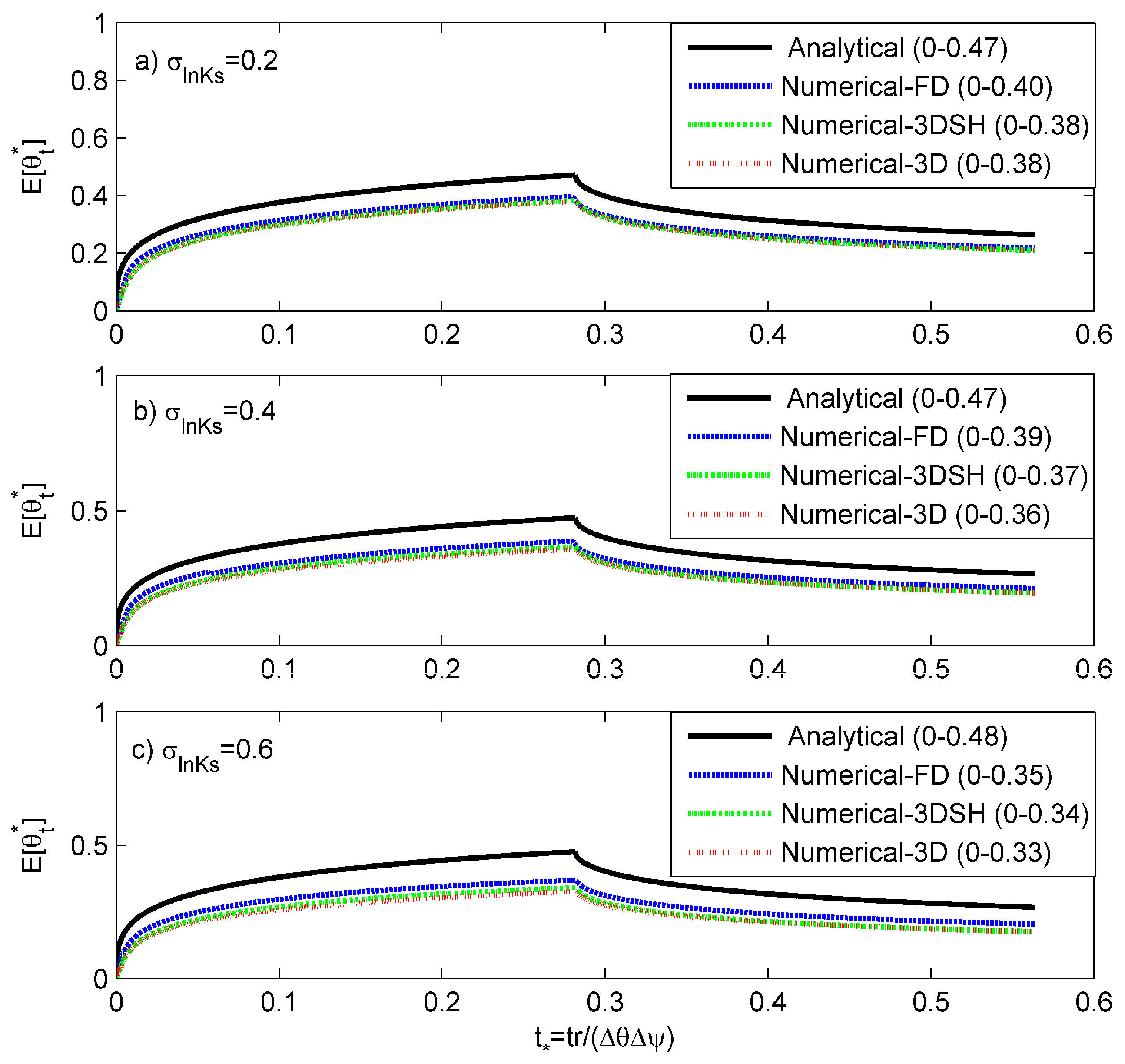
4.1.1. Comparisons with Numerical Results

For the numerical experiment, the following parameter values were considered: ψ b = 34.22   cm , θ r = 0.01 , θ s = 0.415 , θ i = 0.06 , r = 0.5   cm / h , t r = 2   h , λ = 0.91 , μ ln K s = 2 , and σ ln K s = 0.2 in Equations (1) and (2). K s has units of cm / h . Soils with these properties are characterized as sandy loams [45].
The ability of the derived analytical expressions to predict field-scale surface soil moisture variation was validated for different parameter sets against numerical solutions. The mean field-scale surface soil moisture evolution obtained using y e f f in 1-D Richards equation is denoted as “Analytical”. Figure 1 shows comparisons between mean field-scale surface moisture profiles generated for three different values of λ , μ ln K s = 2 , σ ln K s = 0.2 , and r = 0.5   cm / h . A good agreement is observed between the analytical and numerical schemes for all values of λ . Though the analytical expressions are more suited for λ 1 , for smaller values of λ , the conformity between analytical and 3D-numerical solutions is relatively higher for redistribution conditions, and the agreement improves with time. This is probably due to dominance of vertical flow conditions for lower values of λ in 3-D soil fields. The analytical model reproduces the general trend for surface soil moisture evolution as obtained from the three numerical schemes.
Earlier studies have suggested that the sharp front approximations perform better with increase in field-scale variability, as the local errors due to sharp front approximation cancel out during the averaging process. Therefore, the theoretical results are also validated with numerical results for changes in σ ln K s , as shown in Figure 2. The mean saturated hydraulic conductivity, μ ln K s = 2 , λ = 0.91 and other soil parameters are kept constant. A conformity between theoretical model and numerical results is good as in case of σ ln K s = 0.2 and σ ln K s = 0.4 ; however, for σ ln K s = 0.6 the deviation between the results increases for the rainfall duration. For higher variability in σ ln K s , 3-D effects become more prominent, promoting lateral flows thus causing analytical model assumptions to be less met.
The performance of the results from the analytical expressions was also tested for changes in μ ln K s (with other soil parameters kept constant) by comparisons with numerical results. Figure 3 shows comparison between theoretical model results for varying μ ln K s , with σ ln K s = 0.2 , λ = 0.91 and r = 0.5   cm / h . A very good agreement is observed between the theoretical results and the numerical schemes for the rainfall duration as μ ln K s increases. For higher values of μ ln K s , the soil drains faster in independent streamtube columns, thus reducing 3-D lateral effect. The soil moisture content values are higher for low value of μ ln K s = 1.5 , and decrease with increase in μ ln K s . With increase in μ ln K s , a greater fraction of soil-surface is governed by rainfall-limited conditions and pre-ponding conditions dominate at the field-scale over a longer duration. Overall, the expression developed for y e f f in this study reproduces the field-scale surface soil moisture well when compared to numerical results.

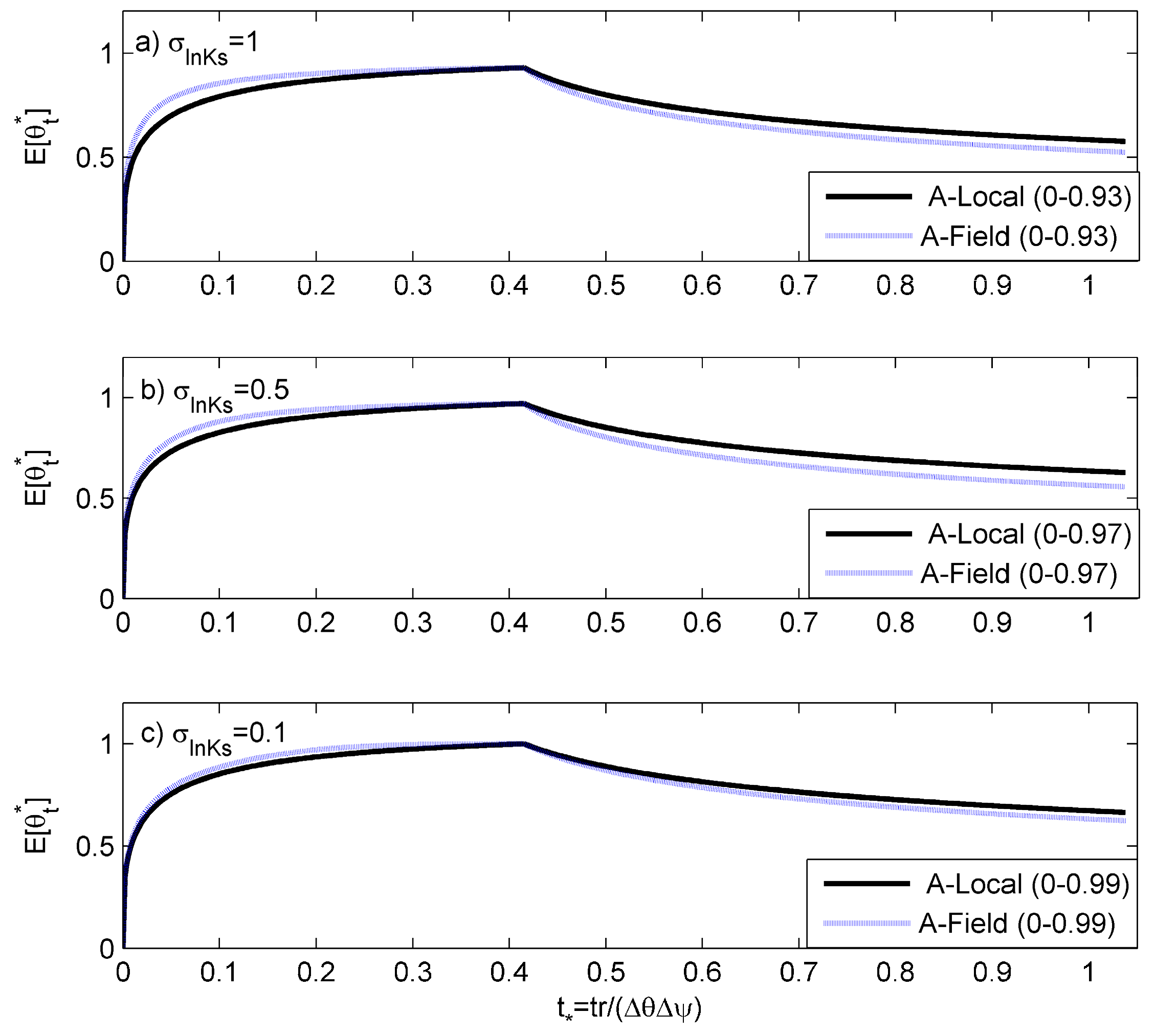
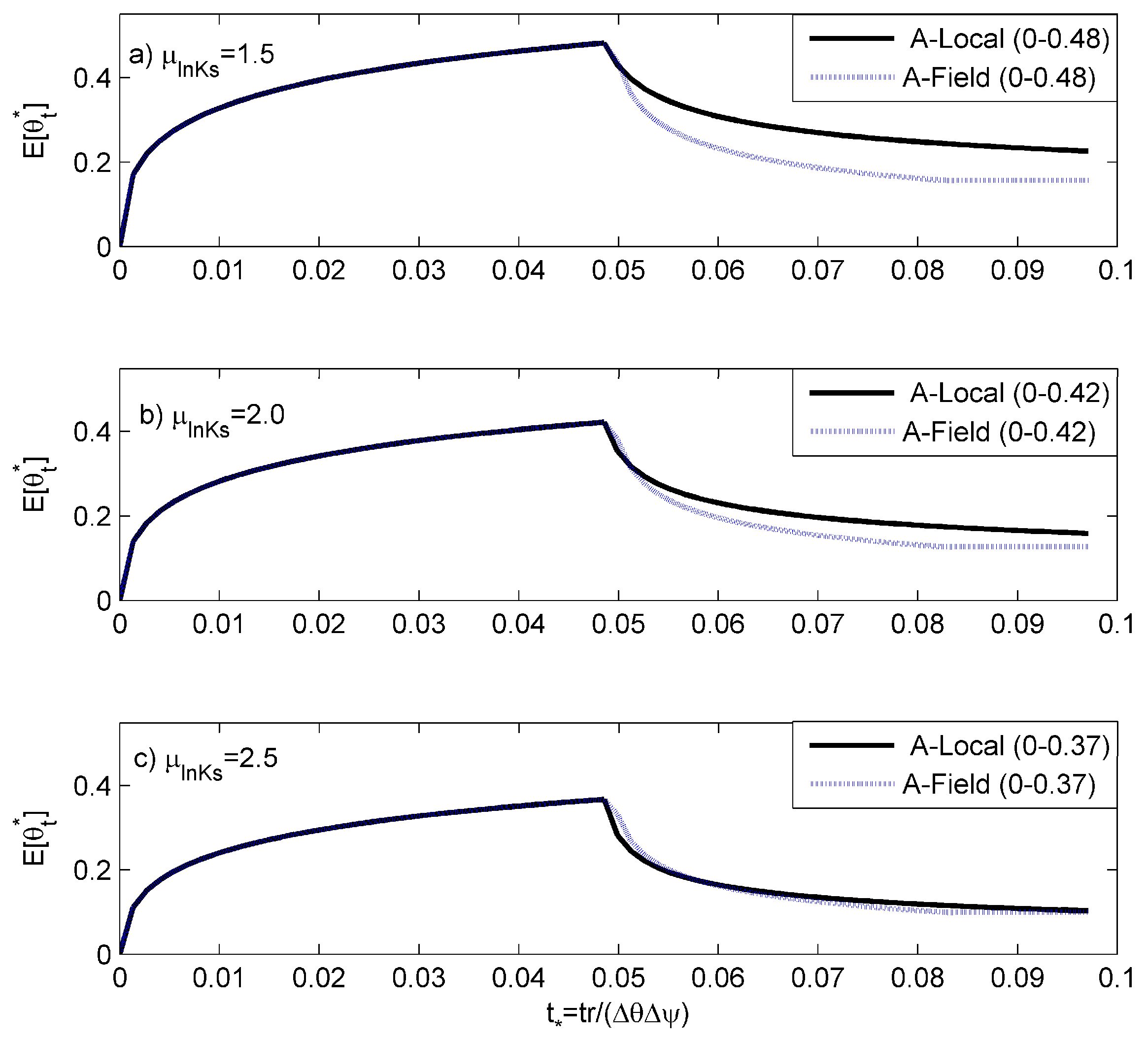
4.1.2. Comparisons with Analytical Results

The mean field-scale surface moisture profiles generated using y e f f are compared with field-scale moisture profiles obtained from the analytical expression (Equations (A6) and (A7) in the Appendix A) proposed by Ojha and Govindaraju [31] for different set of parameters. The mean field-scale surface soil moisture profile generated using y e f f in the analytical expression for local-scale surface soil moisture variation derived from sharp-front approximation (Equations (A1)–(A4)) is denoted as “A-Local”. The mean field-scale surface soil moisture generated using Equations (A6) and (A7) in Appendix A is denoted as “A-Field”.
Figure 4 shows comparisons between the analytical results for varying μ ln K s , with σ ln K s = 0.2 , λ = 0.91 and r = 0.5   cm / h . The other parameters are similar to those used for the numerical experiments. A very good agreement is observed between both the theoretical results (i.e., “A-Local and A-Field”) prior to cessation of rainfall for all values of μ ln K s . As the value of μ ln K s increases, the conformity between the two analytical results increases during redistribution. Further, as the value of μ ln K s increases, a relatively faster drop in the values of E [ θ t ] for redistribution conditions is observed. When K s is high, the soil drains faster, resulting in low moisture content values at the soil surface after rainfall stops.
The proposed analytical expression for y e f f is more suited for sandy-loam soils. However, the efficacy of the developed analytical expression for y e f f in predicting mean field-scale surface soil moisture of soils with very low K s (higher clay content) is also examined. The following parameter values are considered: ψ b = 1   cm , θ r = 0.01 , θ s = 0.415 , θ i = 0.01 , r = 1   cm / h , t r = 1   h , λ = 1.1 , and μ ln K s = 0.5 . Figure 5 shows comparison between theoretical model results for varying σ ln K s . For these soil properties, the exact form of the analytical expression (Equation (14)) for mean field-scale surface soil moisture proposed by Ojha and Govindaraju [31] is used. The soil moisture profile is generated by considering the first 50 terms of the series expansion.
E [ θ t ] = ( t r t r + 1 ) 2 λ / ( 7 λ + 3 ) [ D ] λ / η i = 0 ( λ / η i ) D i [ G ( , [ i ( λ 1 7 λ + 3 ) + λ η ] ) G ( y + K c t r , [ i ( λ 1 7 λ + 3 ) + λ η ] ) ] + ( t r t r + 1 ) 2 λ / ( 7 λ + 3 ) i = 0 ( λ / η i ) D i [ G ( y + K c t r , i ( λ 1 7 λ + 3 ) 2 λ 7 λ + 3 ) G ( K c t r , i ( λ 1 7 λ + 3 ) 2 λ 7 λ + 3 ) ] + [ 1 + η λ ( t r t r 1 + t r ) ] λ / η G ( K c t r , 0 )
where
D = η λ ( t r t r + 1 ) 6 λ + 4 7 λ + 3 [ t t r 1 ] y = ( 1 D ) 7 λ + 3 λ 1
With decrease in σ ln K s , the agreement between “A-Local” and “A-Field” reduces for the rainfall duration. Further, for the same μ ln K s with increase in σ ln K s post-ponding conditions gain prominence, and the magnitude of soil moisture content is high. After the rainfall stops, for a lower value of μ ln K s a gradual decrease in E [ θ t ] is observed, with the rate of decrease reducing with increase in σ ln K s .

4.2. Infiltration Rates

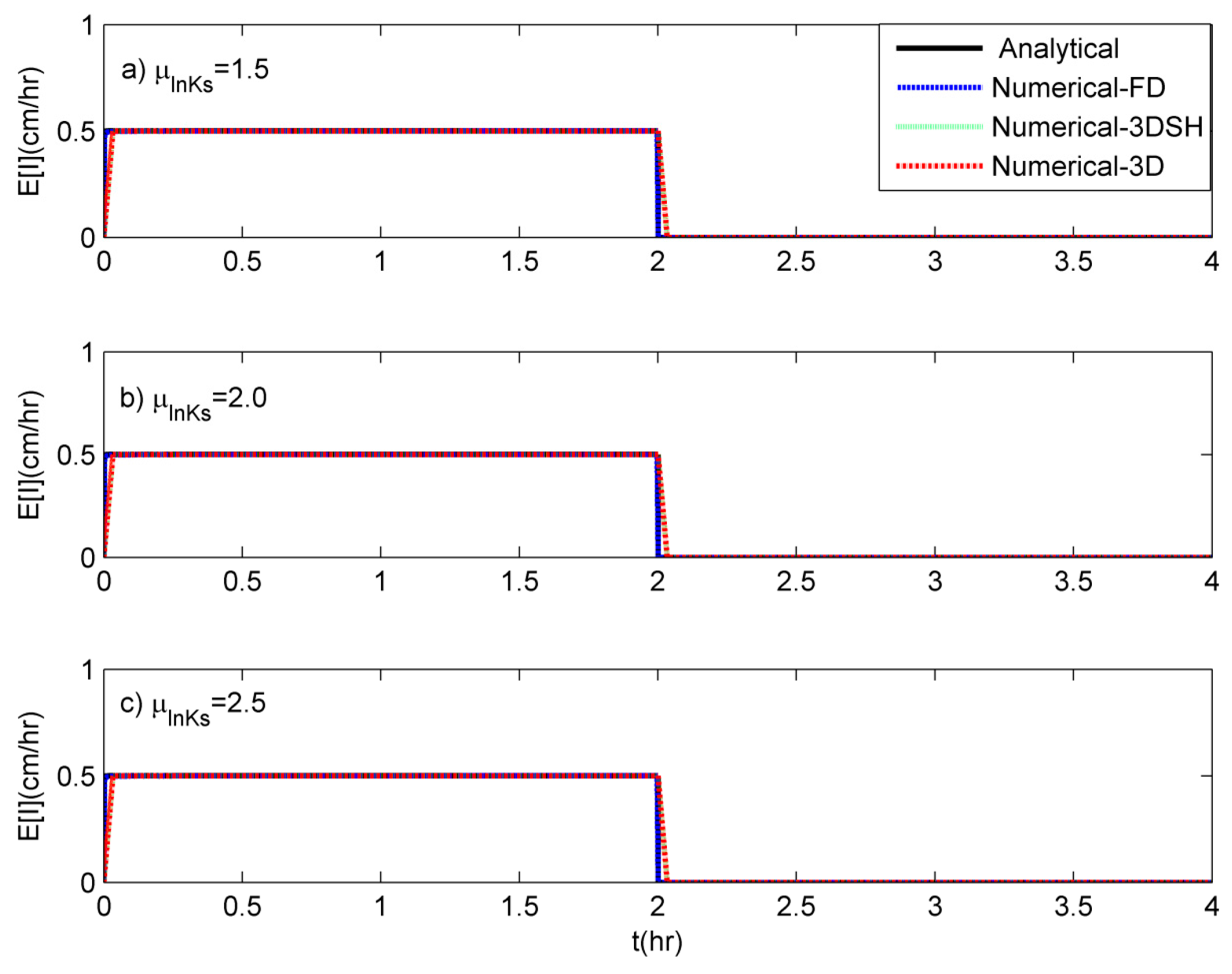
4.2.1. Comparisons with Numerical Results

The parameters used for the numerical validation of mean field-scale surface soil moisture were also utilized to validate the ability of the derived theoretical expression for y e f f (Equation (8)) in predicting mean field-scale infiltration rates. While many cases with different parameter combinations were considered, Figure 6 shows typical results for the case where λ = 0.91 , σ ln K s = 0.2 , and r = 0.5   cm / h , and three different values of mean (a) μ ln K s = 1.5 , (b) μ ln K s = 2.0 and (c) μ ln K s = 2.5 . The theoretical model reproduces the mean field-infiltration rates predicted by the numerical models well. For the rainfall duration, pre-ponding conditions dominate at the field-scale and the E [ I ] is equal to the rainfall rate for different values of μ ln K s .

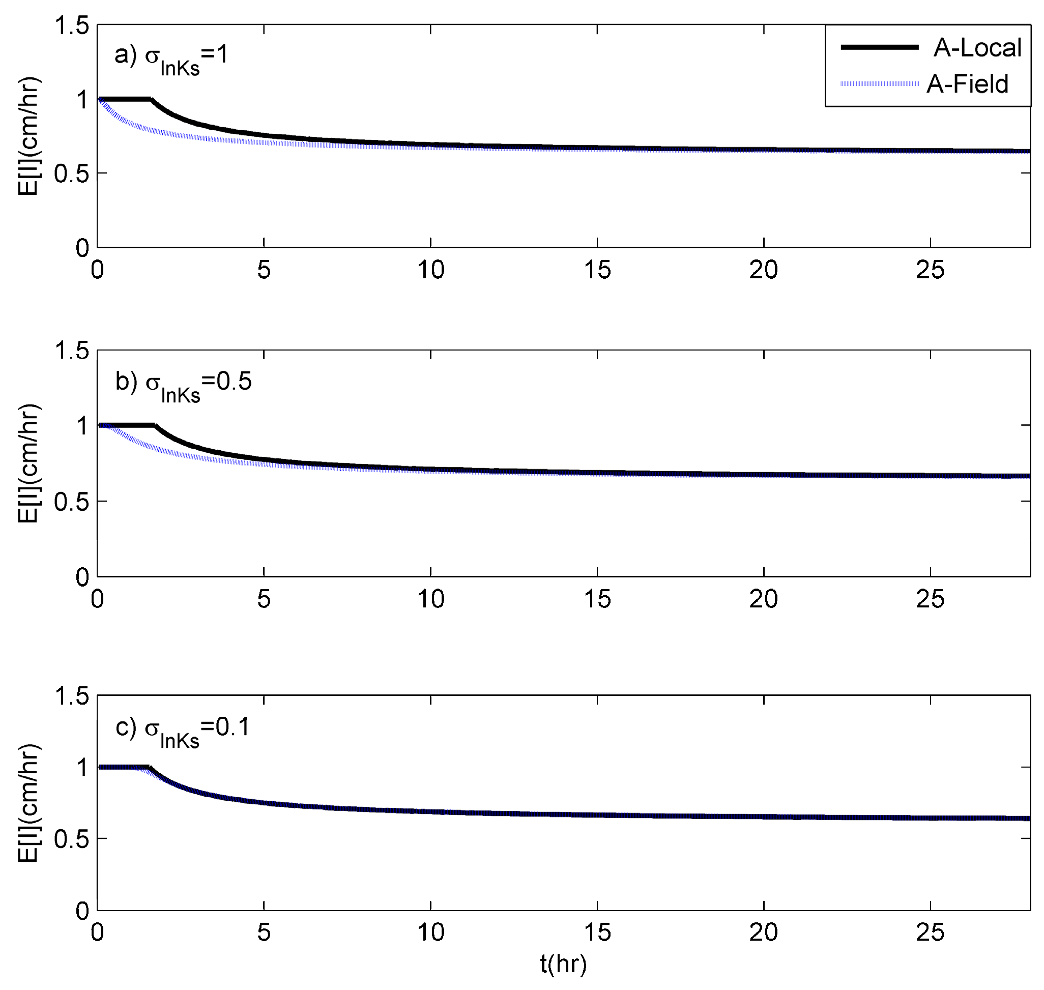
4.2.2. Comparisons with Analytical Results

Similar to surface soil moisture, the mean field-scale infiltration rates generated using y e f f are compared with mean field-scale infiltration rates obtained from the analytical expression (Equation (A8) in the Appendix A) proposed by Govindaraju et al. [4]. The curve for mean field-scale infiltration rates, generated using y e f f in the analytical expression for local-scale infiltration rate variation derived from sharp-front approximation (Equation (3)), is denoted as “A-Local”. The mean field-scale infiltration rates generated using Equation (A8) in Appendix A are denoted as “A-Field”.
Figure 7 shows comparisons between the analytical results for varying σ ln K s , while the other parameter values considered are: ψ b = 1   cm , θ r = 0.01 , θ s = 1 , θ i = 0.01 , r = 1   cm / h , t r = 28   h , λ = 1.1 , and μ ln K s = 0.5 . Using Equation (8), the values of y e f f for constant mean μ ln K s = 0.5 and different standard deviations, σ ln K s = 1 , σ ln K s = 0.5 , σ ln K s = 0.1 are obtained as 0.617, 0.634 and 0.61, respectively. The corresponding time to ponding, t p values are 1.61, 1.73, and 1.56 h, respectively. The parameters were selected such that the ability of the proposed expression for y e f f in predicting the infiltration rates under rainfall at small and large times can be validated. For σ ln K s = 1 , and t 5   h the analytical “A-Local” model over-predicts the mean field-scale infiltration rates (“A-Field”). In case of σ ln K s = 0.5 , initially the “A-Local” and “A-Field” models show very good agreement, but as time progresses for t 5   h the infiltration rate values are higher in magnitude for the “A-Local” model. The mean field-scale infiltration rate values are very well predicted by the “A-Local” model for σ ln K s = 0.1 . Further, at large times, i.e., t , the agreement between infiltration rate values for “A-Local” and “A-Field” is very high. The fractions of the field where pre- and post-ponding conditions exist are governed by the distributional properties of K s and are easily determined. With increase in value of σ ln K s , the control shifts from pre-ponding conditions to post-ponding conditions resulting in a decrease in value of E [ I ] at the field-scale at short times (as observed for “A-Field”). However, as time progresses the entire field experiences post-ponding conditions irrespective of the field-scale variability, and the infiltration rate values match well for both “A-Local” and “A-Field”.

5. Conclusions

In this study, analytical expressions for effective saturated hydraulic conductivity were developed for a single rainfall event. The proposed effective saturated hydraulic conductivity expressions, when combined with 1-D Richards equation or local-scale simplified models based on sharp front approximation can be utilized to determine field-scale mean-surface moisture content and infiltration rates. The dimensionless equations for effective saturated hydraulic conductivity were derived from a sharp front model. Comparisons with 1-D Monte Carlo-based simulations, 3-D numerical simulations, and analytical results proposed by Govindaraju et al. [4] and Ojha and Govindaraju [31] showed that the proposed theory provides a simple alternative to determining the surface soil moisture and infiltration rates in the field for a single rainfall event, with insights into role of rainfall- and soil-controlled behavior for pre- and post-ponded conditions. The theoretical model readily describes field-scale surface soil moisture and infiltration rates where otherwise extensive amount of numerical computations would be needed.
Given the assumptions, the proposed analytical model for infiltration rates is better suited for recharge rates that are significantly greater than the mean saturated hydraulic conductivity. The field size should be much larger than the horizontal correlation length scale for meaningful spatial averages. The analytical model over-predicts the infiltration rate values at short time as field-scale variability increases. The numerical computation of the right hand side of Equation (7) also needs special care as pointed out by van Genuchten [46]. Nevertheless, the theoretical model proposed in this study provides a useful alternative for describing mean field-scale surface soil moisture and infiltration rates in heterogeneous unsaturated soils.
As noted, expressions for effective properties (Equations (8) and (11)) are better suited for sandy loam soils where the approximation of a sharp wetting front is better met than clayey soils where the wetting front tends to extend over greater depths. The assumption of initially dry soils allows us to neglect the very small conductivity values associated with initial conditions. Our experience with numerical simulations shows that these are not strict constraints, as the local deviations tend to cancel out in the face of variability resulting from field scale heterogeneity.
There are important implications when using effective saturated hydraulic conductivity to simulate field-scale behavior. First, the effective value is dependent on the rainfall intensity (see also KINEROS2) and not solely a function of K s variability as one would expect from using equivalent media theories. This is a consequence of the infiltration process. Thus, if no rainfall excess and subsequent runoff are generated over a field under a rainfall event, the effective value of K s is not identifiable as any value greater than rainfall intensity will yield the same result. If the rainfall intensity is varying in time, then the effective conductivity to be used in Green-Ampt model for field-scale infiltration rate will also need to be varying with time. This is a more complex problem and deserves future attention.
A second important consideration revealed here is the need for one effective K s value to replicate field-scale runoff data, and another one for reproducing field-scale surface soil moisture. This is an artifact of the use of the Green-Ampt model, an approximation that is being used to mimic field-scale behavior as determined by Richards equation. Specifically, the effective K s from runoff data does not replicate field-scale surface moisture and vice versa. Conversely, if runoff data are used to calibrate for an effective K s value, this estimate will be different from the value obtained from calibrating an effective K s value based on estimates of surface soil moisture at numerous locations. If runoff and surface soil moisture data are used together to estimate effective K s values, then it is likely that such values will not yield good calibration and validation statistics. This is a common limitation in hydrology, and reaffirms that calibration yields effective values, but these values may not be intrinsic medium properties—this problem remains as a challenge.

Author Contributions

Richa Ojha, Corrado Corradini, Renato Morbidelli and Rao S. Govindaraju worked on the conceptualization and mathematical development. Richa Ojha worked on the numerical computations. All authors contributed to writing of the paper.

Conflicts of Interest

The authors declare no conflict of interest.

Appendix A. Expressions for Soil Moisture Content and Infiltration Rate

Appendix A.1. Soil Moisture Content Variation for Initially Dry Soils

Appendix A.1.1. Local-Scale

Case A: Ponding conditions are achieved ( r > K s , and rainfall duration t r > t p )
At local-scale, for pre-ponding conditions ( t < t p ), the water content from Darcy’s law and continuity equation can be described by Equation (A1).
θ t = { 1 y [ t t r + 1 ] } 2 λ / ( 7 λ + 3 )
whereas for post-ponding conditions
θ t = 1
For redistribution condition ( r = 0 ; t > t r ), from Ojha and Govindaraju [31], the soil moisture content variation for rainfall events of smaller duration can be expressed as,
θ t = { 1 + η λ [ t t r 1 + t r ] } λ / η
Case B: Ponded conditions are not achieved ( r < K s , or r > K s but t r < t p )
The soil moisture prior to cessation of rainfall can be described by Equation (A1); however, the water content in this case asymptotically approaches a maximum value θ max .
For redistribution condition, from Charbeneau [47], the moisture content variation is expressed as,
θ t = θ t r [ 1 + y ( θ t r ) η / λ η λ ( t t r 1 ) ] λ / η

Appendix A.1.2. Field-Scale Solution

Considering that the saturated hydraulic conductivity y follows a log-normal distribution at field-scale the mean-field scale moisture is expressed as,
E [ θ t ] = 0 θ t f y ( y ) d y
Utilizing Equations (A1), (A2) and (A5) mean field-scale soil moisture evolution prior to cessation of rainfall ( t t r ) is evaluated as
E [ θ t ] = ( t t + 1 ) 2 λ / ( 7 λ + 3 ) [ G ( , 2 λ 7 λ + 3 ) G ( K c t , 2 λ 7 λ + 3 ) ] + G ( K c t , 0 )
Similarly, for sandy loam soils the mean field-scale soil moisture evolution after cessation of rainfall ( t > t r ) can be evaluated by considering average of the leading terms obtained from binomial expansion of Equation (A4), and Equations (A3) and (A5)
E [ θ t ] = 0.5 ( t r t r + 1 ) 2 λ / ( 7 λ + 3 ) [ D ] λ / η [ G ( , λ η ) G ( y + K c t r , λ η ) ] + 0.5 ( t r t r + 1 ) 2 λ / ( 7 λ + 3 ) [ G ( y + K c t r , 2 λ 7 λ + 3 ) G ( K c t r , 2 λ 7 λ + 3 ) ] + [ 1 + η λ ( t t r 1 + t r ) ] λ / η G ( K c t r , 0 )

Appendix A.2. Expected Field-Scale InfiltrationRates

Utilizing Equation (3) in the manuscript and considering log-normal distribution of saturated hydraulic conductivity, the field-scale infiltration rate can be expressed as,
E [ I ( F ) ] = r [ 1 G Y ( K c , 0 ) ] + ψ Δ θ + F F G Y ( K c , 1 )

References

  1. Brocca, L.; Melone, F.; Moramarco, T.; Morbidelli, R. Spatial-temporal variability of soil moisture and its estimation across scales. Water Resour. Res. 2010, 46. [Google Scholar] [CrossRef]
  2. Corradini, C.; Flammini, A.; Morbidelli, R.; Govindaraju, R.S. A conceptual model for infiltration in two-layered soils with a more permeable upper layer: From local to field scale. J. Hydrol. 2011, 410, 62–72. [Google Scholar] [CrossRef]
  3. Srivastava, R.; Yeh, T.-C.J. Analytical solutions for one-dimensional, transient infiltration toward the water table in homogeneous and layered soils. Water Resour. Res. 1991, 27, 753–762. [Google Scholar] [CrossRef]
  4. Govindaraju, R.S.; Morbidelli, R.; Corradini, C. Areal Infiltration Modeling over Soils with Spatially Correlated Hydraulic Conductivities. J. Hydrol. Eng. 2001, 6, 150–158. [Google Scholar] [CrossRef]
  5. Govindaraju, R.S.; Corradini, C.; Morbidelli, R. A semi-analytical model of expected areal-average infiltration under spatial heterogeneity of rainfall and soil saturated hydraulic conductivity. J. Hydrol. 2006, 316, 184–194. [Google Scholar] [CrossRef]
  6. Ojha, R.; Prakash, A.; Govindaraju, R.S. Local- and field-scale stochastic-advective vertical solute transport in horizontally heterogeneous unsaturated soils. Water Resour. Res. 2014, 50. [Google Scholar] [CrossRef]
  7. Western, A.W.; Grayson, R.B.; Blöschl, G. Scaling of Soil Moisture: A Hydrologic Perspective. Annu. Rev. Earth Planet. Sci. 2002, 30, 149–180. [Google Scholar] [CrossRef]
  8. Grayson, R.B.; Western, A.W. Towards areal estimation of soil water content from point measurements: Time and space stability of mean response. J. Hydrol. 1998, 207, 68–82. [Google Scholar] [CrossRef]
  9. Lai, J.; Ren, L. Estimation of effective hydraulic parameters in heterogeneous soils at field scale. Geoderma 2016, 264, 28–41. [Google Scholar] [CrossRef]
  10. Vereecken, H.; Kasteel, R.; Vanderborght, J.; Harter, T. Upscaling Hydraulic Properties and Soil Water Flow Processes in Heterogeneous Soils. Vadose Zone J. 2007, 6, 1–28. [Google Scholar] [CrossRef]
  11. Sadeghi, M.; Tuller, M.; Gohardoust, M.R.; Jones, S.B. Column-scale unsaturated hydraulic conductivity estimates in coarse-textured homogeneous and layered soils derived under steady-state evaporation from a water table. J. Hydrol. 2014, 519, 1238–1248. [Google Scholar] [CrossRef]
  12. Bolster, D.; Dentz, M.; Carrera, J. Effective two-phase flow in heterogeneous media under temporal pressure fluctuations. Water Resour. Res. 2009, 45. [Google Scholar] [CrossRef]
  13. Liu, Z.; Zha, Y.; Yang, W.; Kuo, Y.-M.; Yang, J. Large-Scale Modeling of Unsaturated Flow by a Stochastic Perturbation Approach. Vadose Zone J. 2016, 15. [Google Scholar] [CrossRef]
  14. Mantoglou, A.; Gelhar, L.W. Stochastic modeling of large-scale transient unsaturated flow systems. Water Resour. Res. 1987, 23, 37–46. [Google Scholar] [CrossRef]
  15. Ünlü, K.; Nielsen, D.R.; Biggar, J.W.; Morkoc, F. Statistical Parameters Characterizing the Spatial Variability of Selected Soil Hydraulic Properties. Soil Sci. Soc. Am. J. 1990, 54, 1537. [Google Scholar] [CrossRef]
  16. Zhang, D. Nonstationary stochastic analysis of transient unsaturated flow in randomly heterogeneous media. Water Resour. Res. 1999, 35, 1127–1141. [Google Scholar] [CrossRef]
  17. Bresler, E.; Dagan, G. Unsaturated flow in spatially variable fields: 2. Application of water flow models to various fields. Water Resour. Res. 1983, 19, 421–428. [Google Scholar] [CrossRef]
  18. Dagan, G.; Bresler, E. Unsaturated flow in spatially variable fields: 1. Derivation of models of infiltration and redistribution. Water Resour. Res. 1983, 19, 413–420. [Google Scholar] [CrossRef]
  19. Mohanty, B.P.; Zhu, J.; Mohanty, B.P.; Zhu, J. Effective Hydraulic Parameters in Horizontally and Vertically Heterogeneous Soils for Steady-State Land–Atmosphere Interaction. J. Hydrometeorol. 2007, 8, 715–729. [Google Scholar] [CrossRef]
  20. Zhu, J.; Mohanty, B.P. Upscaling of soil hydraulic properties for steady state evaporation and infiltration. Water Resour. Res. 2002, 38, 17-1–17-13. [Google Scholar] [CrossRef]
  21. Zhu, J.; Mohanty, B.P.; Das, N.N. On the Effective Averaging Schemes of Hydraulic Properties at the Landscape Scale. Vadose Zone J. 2006, 5, 308–316. [Google Scholar] [CrossRef]
  22. Foussereau, X.; Graham, W.D.; Rao, P.S.C. Stochastic analysis of transient flow in unsaturated heterogeneous soils. Water Resour. Res. 2000, 36, 891–910. [Google Scholar] [CrossRef]
  23. Ward, A.L.; Zhang, Z.F.; Gee, G.W. Upscaling unsaturated hydraulic parameters for flow through heterogeneous anisotropic sediments. Adv. Water Resour. 2006, 29, 268–280. [Google Scholar] [CrossRef]
  24. Ye, M.; Khaleel, R.; Yeh, T.-C.J. Stochastic analysis of moisture plume dynamics of a field injection experiment. Water Resour. Res. 2005, 41. [Google Scholar] [CrossRef]
  25. Yeh, T.-C.J.; Ye, M.; Khaleel, R. Estimation of effective unsaturated hydraulic conductivity tensor using spatial moments of observed moisture plume. Water Resour. Res. 2005, 41. [Google Scholar] [CrossRef]
  26. Nietsch, S.L.; Arnold, J.G.; Kiniry, J.R.; Williams, J.R. SWAT User Documentation, Version 2005. 2005. Available online: http://swat.tamu.edu/media/1292/swat2005theory.pdf (accessed on 17 February 2017).
  27. Downer, C.; Ogden, F. GSSHA: Model to simulated diverse streamflow producing processes. J. Hydrol. Eng. 2004, 9, 161–174. [Google Scholar] [CrossRef]
  28. KINEROS2: A Kinematic Runoff and Erosion Model. Available online: http://www.tucson.ars.ag.gov/kineros (accessed on 14 February 2017).
  29. Yang, J.; Zhang, D.; Lu, Z. Stochastic analysis of saturated–unsaturated flow in heterogeneous media by combining Karhunen-Loeve expansion and perturbation method. J. Hydrol. 2004, 294, 18–38. [Google Scholar] [CrossRef]
  30. Ojha, R.; Morbidelli, R.; Saltalippi, C.; Flammini, A.; Govindaraju, R.S. Scaling of surface soil moisture over heterogeneous fields subjected to a single rainfall event. J. Hydrol. 2014, 516. [Google Scholar] [CrossRef]
  31. Ojha, R.; Govindaraju, R.S. A physical scaling model for aggregation and disaggregation of field-scale surface soil moisture dynamics. Chaos 2015, 25. [Google Scholar] [CrossRef] [PubMed]
  32. Chen, Z.; Govindaraju, R.S.; Kavvas, M.L. Spatial averaging of unsaturated flow equations under infiltration conditions over areally heterogeneous fields 2. Numerical simulations. Water Resour. Res. 1994, 30, 535–548. [Google Scholar] [CrossRef]
  33. Chen, Z.; Govindaraju, R.S.; Kavvas, M.L. Spatial averaging of unsaturated flow equations under infiltration conditions over areally heterogeneous fields: 1. Development of models. Water Resour. Res. 1994, 30, 523–533. [Google Scholar] [CrossRef]
  34. Govindaraju, R.S.; Or, D.; Kavvas, M.L.; Rolston, D.E.; Biggar, J. Error analyses of simplified unsaturated flow models under large uncertainty in hydraulic properties. Water Resour. Res. 1992, 28, 2913–2924. [Google Scholar] [CrossRef]
  35. Destouni, G. The effect of vertical soil heterogeneity on field scale solute flux. Water Resour. Res. 1992, 28, 1303–1309. [Google Scholar] [CrossRef]
  36. Leij, F.J.; Sciortino, A.; Haverkamp, R.; Soria Ugalde, J.M. Aggregation of vertical flow in the vadose zone with auto- and cross-correlated hydraulic properties. J. Hydrol. 2007, 338, 96–112. [Google Scholar] [CrossRef]
  37. Russo, D. Field-scale transport of interacting solutes through the unsaturated zone: 1. Analysis of the spatial variability of the transport properties. Water Resour. Res. 1989, 25, 2475–2485. [Google Scholar] [CrossRef]
  38. Russo, D. Field-scale transport of interacting solutes through the unsaturated zone: 2. Analysis of the spatial variability of the field response. Water Resour. Res. 1989, 25, 2487–2495. [Google Scholar] [CrossRef]
  39. Kavvas, M.L.; Chen, Z.Q.; Govindaraju, R.S.; Rolston, D.E.; Koos, T.; Karakas, A.; Or, D.; Jones, S.; Biggar, J. Probability Distribution of Solute Travel Time for Convective Transport in Field-Scale Soils Under Unsteady and Nonuniform Flows. Water Resour. Res. 1996, 32, 875–889. [Google Scholar] [CrossRef]
  40. Russo, D.; Bresler, E. A univariate versus a multivariate parameter distribution in a stochastic-conceptual analysis of unsaturated flow. Water Resour. Res. 1982, 18, 483–488. [Google Scholar] [CrossRef]
  41. Nielsen, D.; Biggar, J.; Erh, K. Spatial variability of field-measured soil-water properties. Hilgardia 1973, 42, 215–259. [Google Scholar] [CrossRef]
  42. Brooks, R.J.; Corey, A.T. Hydraulic Properties of Porous Media; Hydrol. Pap. 3; Colorado State University: Fort Collins, CO, USA, 1964; 27p. [Google Scholar]
  43. Chow, V.T.; Maidment, D.R.; Mays, L.W.; Chow, V.T.; Maidment, D.R.; Mays, L.W. Applied Hydrology; McGraw-Hill: New York, NY, USA, 1988. [Google Scholar]
  44. Simůnek, J.; Genuchten, M.T.V.; Sejna, M. The Hydrus Soft-Ware Package for Simulating Two- and Three-Dimensional Movement of Water, Heat, and Multiple Solutes in Variably-Saturated Media: Technical Manual, version 1.0; PC-Progress: Prague, Czech Republic, 2006. [Google Scholar]
  45. Rawls, W.J.; Brakensiek, D.L.; Miller, N. Green-ampt Infiltration Parameters from Soils Data. J. Hydraul. Eng. 1983, 109, 62–70. [Google Scholar] [CrossRef]
  46. Van Genuchten, M.T. Convective-dispersive transport of solutes involved in sequential first-order decay reactions. Comput. Geosci. 1985, 11, 129–147. [Google Scholar] [CrossRef]
  47. Charbeneau, R.J. Groundwater Hydraulics and Pollutant Transport; Prentice Hall: Upper Saddle River, NJ, USA, 2000; pp. 206–211. [Google Scholar]
Figure 1. Comparison of field-scale evolution of mean surface soil moisture content, E [ θ t ] , obtained from analytical and numerical schemes, for r = 0.5   cm / h , μ ln K s = 2 , and σ ln K s = 0.2 , (a) λ = 0.313 ; (b) λ = 0.616 and (c) λ = 0.91 . For all the figures, (1) Analytical: Flow field obtained from numerical solution of 1-D Richards equation for y e f f ; (2) Numerical-3DSH: 3-D numerical solutions obtained using Hydrus-3D for spatially heterogeneous and vertically homogeneous soils; (3) Numerical-3D: 3-D numerical solutions obtained using Hydrus-3D for fully heterogeneous field; (4) Numerical-FD: Numerical solutions obtained using Monte-Carlo simulation. The values in the legend denote the range of variation of E [ θ t ] for that particular scheme.
Water 09 00134 g001
Figure 2. Comparison of field-scale evolution of mean surface soil moisture content obtained from analytical and numerical schemes, E [ θ t ] for μ ln K s = 2 , r = 0.5   cm / h and λ = 0.91 , (a) σ ln K s = 0.2 ; (b) σ ln K s = 0.4 , and (c) σ ln K s = 0.6 . For all the figures, (1) Analytical: Flow field obtained from numerical solution of 1-D Richards equation for y e f f ; (2) Numerical-3DSH: 3-D numerical solutions obtained using Hydrus-3D for spatially heterogeneous and vertically homogeneous soils; (3) Numerical-3D: 3-D numerical solutions obtained using Hydrus-3D for fully heterogeneous field; (4) Numerical-FD: Numerical solutions obtained using Monte-Carlo simulation. The values in the legend denote the range of variation of E [ θ t ] for that particular scheme.
Water 09 00134 g002
Figure 3. Comparison of field-scale evolution of mean surface soil moisture content obtained from analytical and numerical schemes, E [ θ t ] for r = 0.5   cm / h , σ ln K s = 0.2 , and λ = 0.91 , (a) μ ln K s = 1.5 ; (b) μ ln K s = 2 and (c) μ ln K s = 2.5 . For all the figures, (1) Analytical: Flow field obtained from numerical solution of 1-D Richards equation for y e f f ; (2) Numerical-3DSH: 3-D numerical solutions obtained using Hydrus-3D for spatially heterogeneous and vertically homogeneous soils; (3) Numerical-3D: 3-D numerical solutions obtained using Hydrus-3D for fully heterogeneous field; (4) Numerical-FD: Numerical solutions obtained using Monte-Carlo simulation. The values in the legend denote the range of variation of E [ θ t ] for that particular scheme.
Water 09 00134 g003
Figure 4. Comparison of field-scale evolution of mean surface soil moisture content obtained from analytical schemes, E [ θ t ] for r = 0.5   cm / h , t r = 2   h , σ ln K s = 0.2 , and λ = 0.91 , (a) μ ln K s = 1.5 ; (b) μ ln K s = 2 and (c) μ ln K s = 2.5 . For all the figures, (1) A-Local: Moisture profile obtained from local-scale analytical expression for surface soil moisture evolution derived using sharp front approximation for y e f f ; (2) A-Field: Moisture profile obtained from analytical expression for field-scale surface soil moisture evolution. The values in the legend denote the range of variation of E [ θ t ] for that particular scheme.
Water 09 00134 g004
Figure 5. Comparison of field-scale evolution of mean surface soil moisture content obtained from analytical schemes, E [ θ t ] for r = 1   cm / h , t r = 1   h , μ ln K s = 0.5 and λ = 1.1 , (a) σ ln K s = 1 ; (b) σ ln K s = 0.5 ; and (c) σ ln K s = 0.1 . For all the figures, (1) A-Local: Moisture profile obtained from local-scale analytical expression for surface soil moisture evolution derived using sharp front approximation for y e f f ; (2) A-Field: Moisture profile obtained from analytical expression for field-scale surface soil moisture evolution.
Water 09 00134 g005
Figure 6. Comparison of field-scale evolution of infiltration rates, obtained from analytical and numerical schemes, E [ I ] for r = 0.5   cm / h , σ ln K s = 0.2 , and λ = 0.91 , (a) μ ln K s = 1.5 ; (b) μ ln K s = 2.0 and (c) μ ln K s = 2.5 . (1) Analytical: Flow field obtained from numerical solution of 1-D Richards equation for y e f f ; (2) Numerical-3DSH: 3-D numerical solutions obtained using Hydrus-3D for spatially heterogeneous and vertically homogeneous soils; (3) Numerical-3D: 3-D numerical solutions obtained using Hydrus-3D for fully heterogeneous field; (4) Numerical-FD: Numerical solutions obtained using Monte-Carlo simulation.
Water 09 00134 g006
Figure 7. Comparison of field-scale evolution of infiltration rates obtained from analytical schemes, E [ I ] for μ ln K s = 0.5 , r = 1   cm / h and λ = 1.1 , (a) σ ln K s = 1 ; (b) σ ln K s = 0.5 ; and (c) σ ln K s = 0.1 . For all the figures, (1) A-Local: Infiltration rates obtained from local-scale analytical expression for infiltration from sharp front approximation for y e f f ; (2) A-Field: Infiltration rates obtained from analytical expression for field-scaleinfiltration evolution.
Water 09 00134 g007

