Contemporary and Future Characteristics of Precipitation Indices in the Kentucky River Basin

Abstract
:1. Introduction
2. Materials and Methods
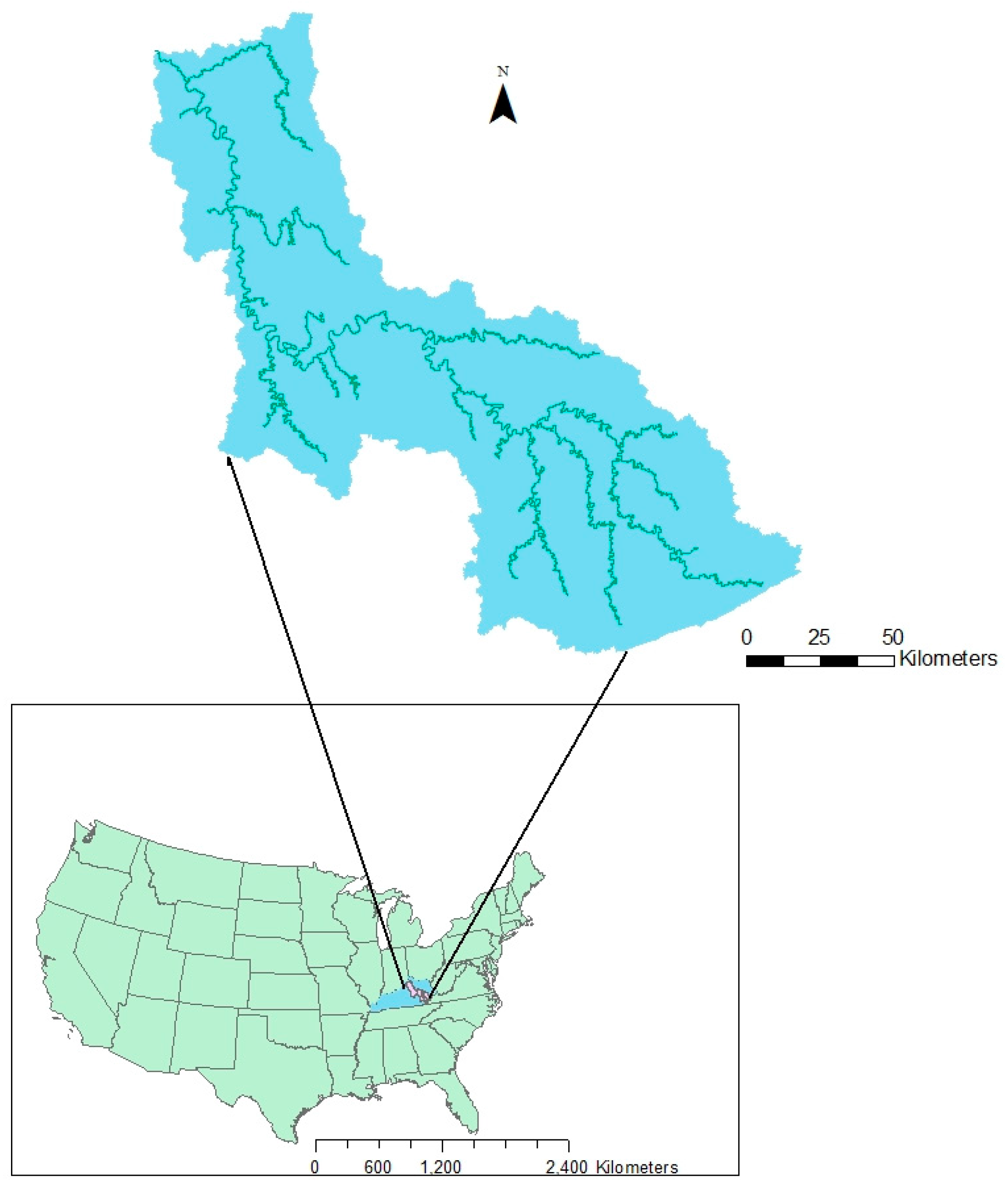
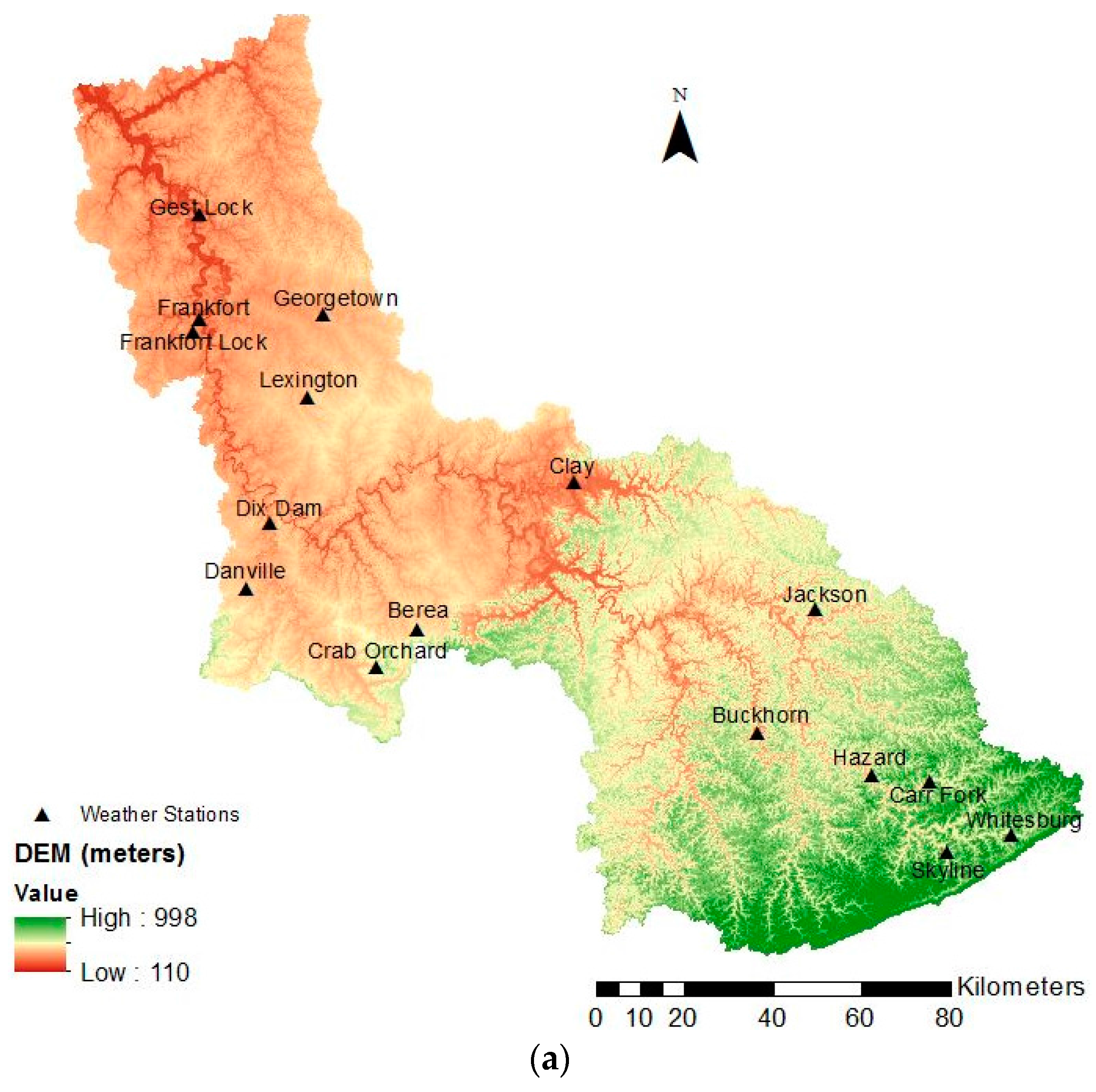
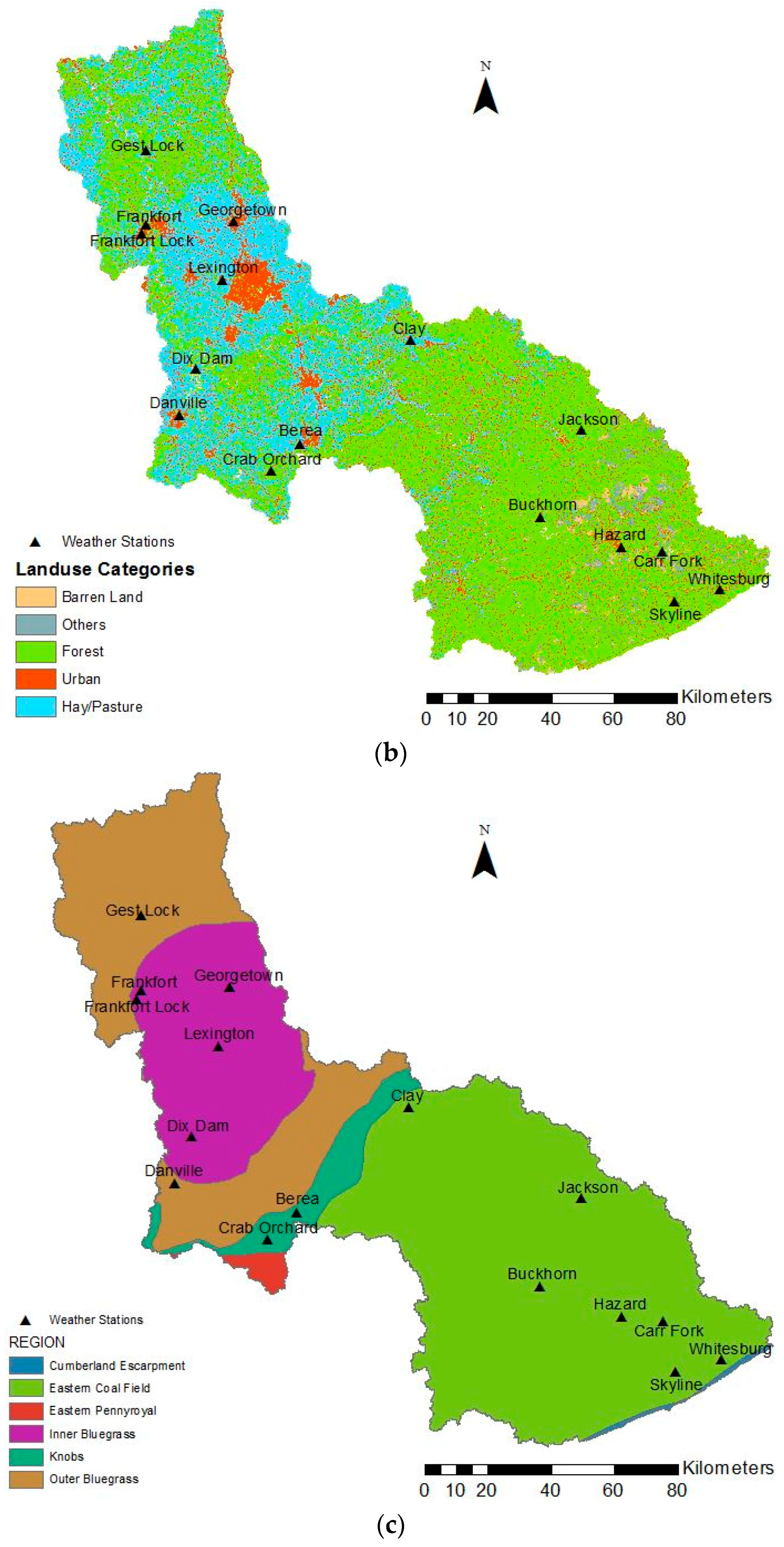
2.1. Study Area
2.2. Data Collection and Quality Assessment
2.3. Future Climate Data Compilation
2.4. Extreme Precipitation Indices
- The total precipitation in wet days (days having ≥1 mm precipitation) (PRCPTOT, mm)
- The maximum length of dry periods (CDD, days)
- The maximum length of wet periods (CWD days)
- Number of days in a year with precipitation ≥20 mm (R20mm, days)
- The annual maximum precipitation over five consecutive days (RX5day, mm)
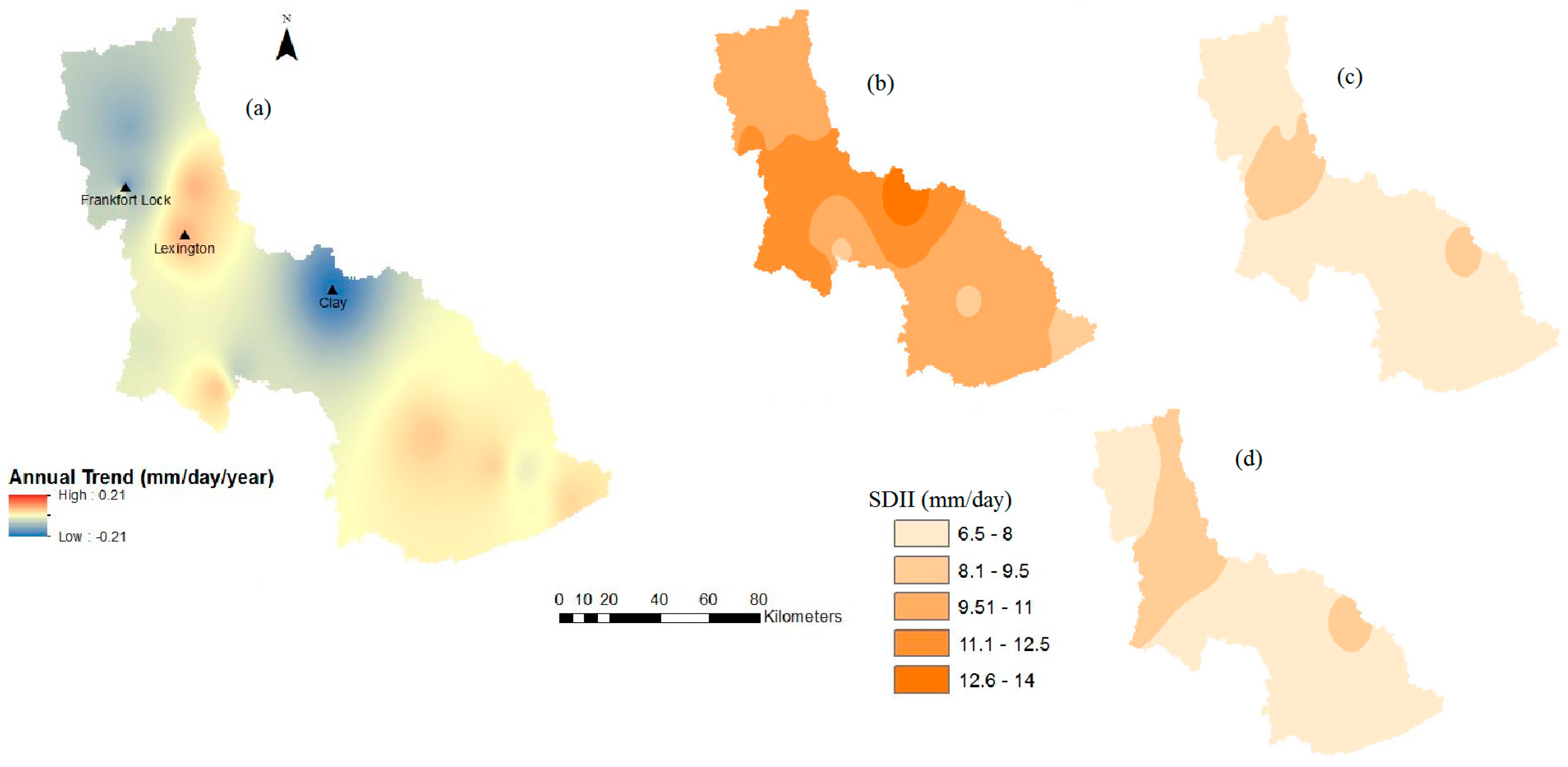
- The simple daily precipitation intensity (SDII, mm/day), calculated as PRCPTOT/(number of wet days)
2.5. Trend Detection
3. Results and Discussion
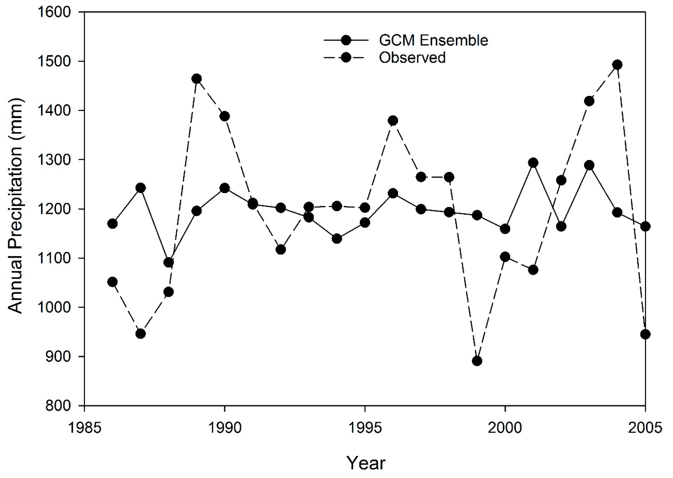
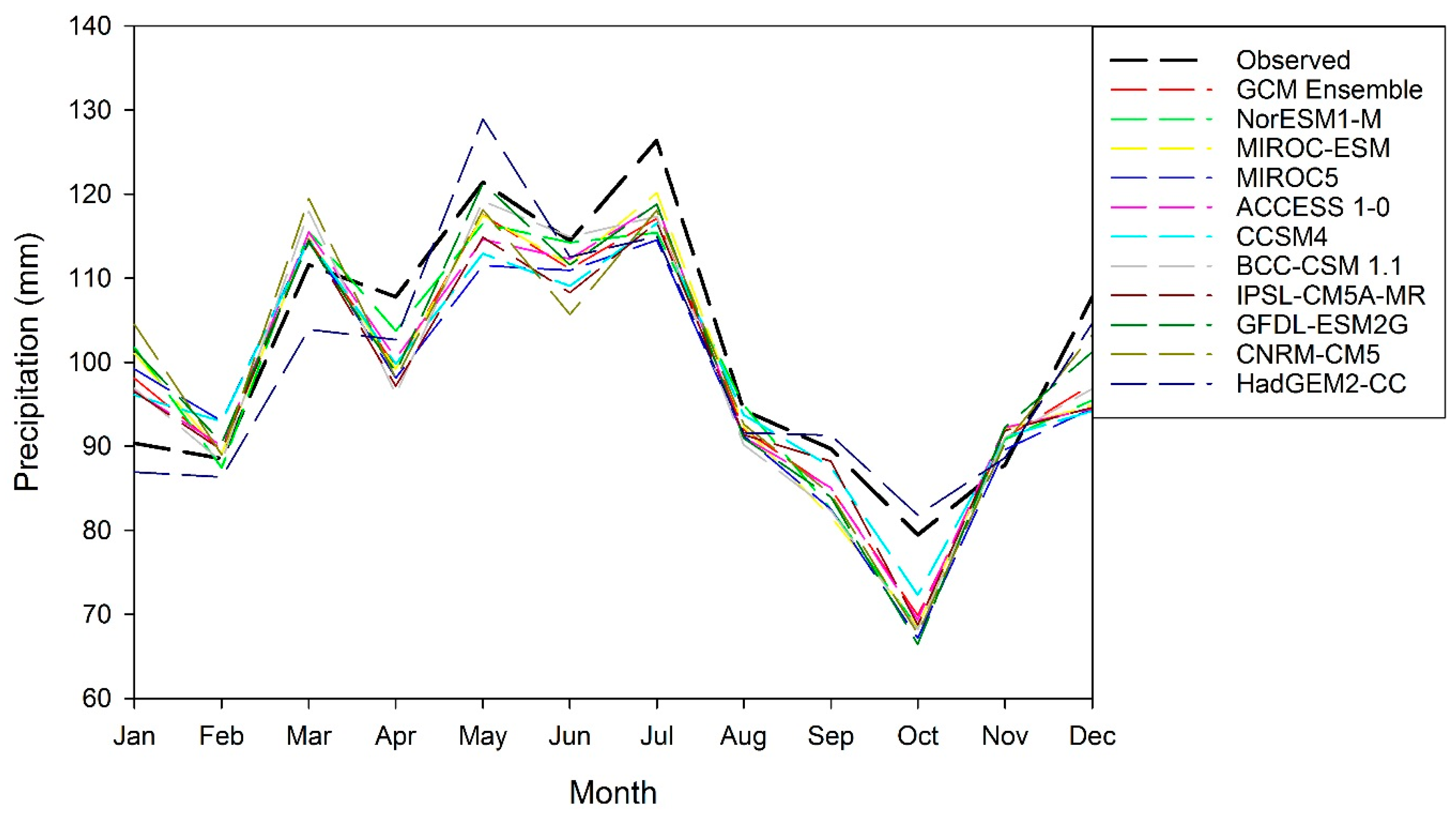
3.1. GCM Performance Evaluation
3.2. Trend Analysis of Extreme Indices
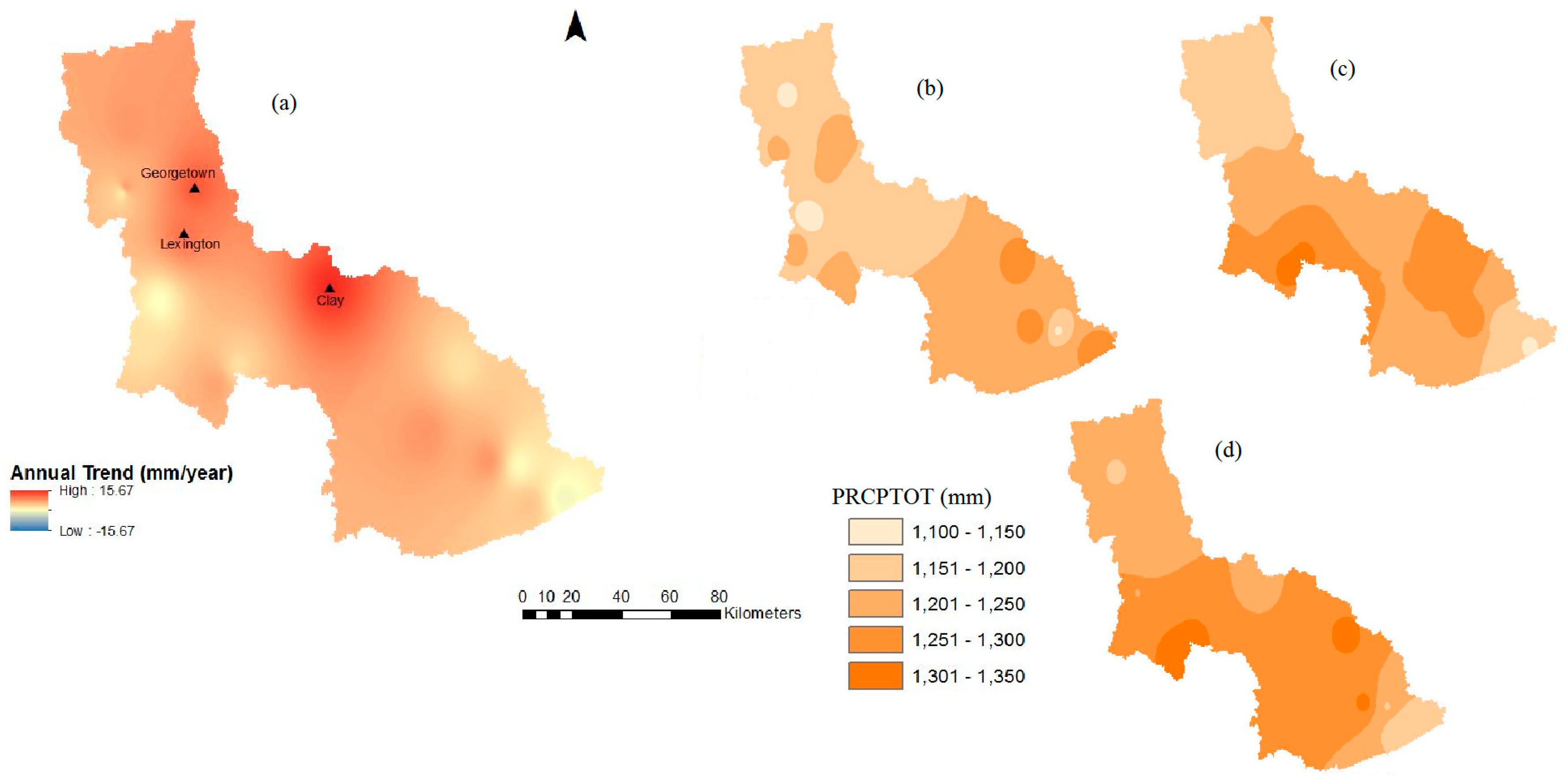
3.3. PRCPTOT
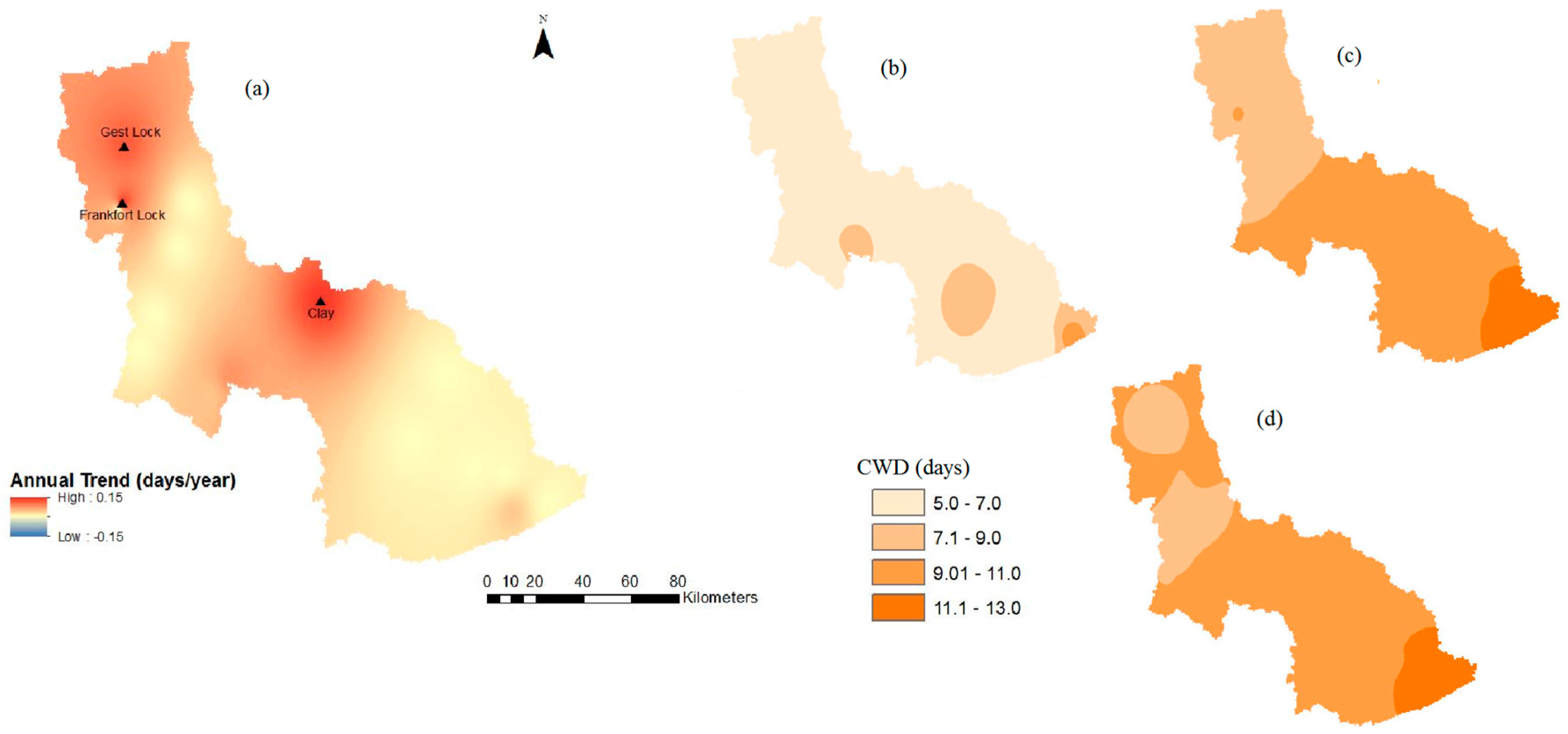
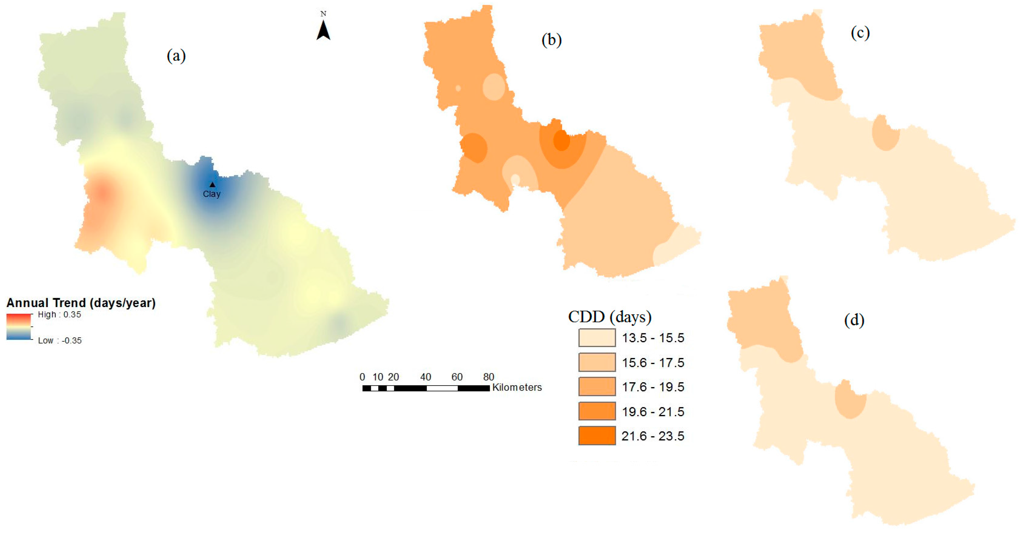
3.4. CDD and CWD
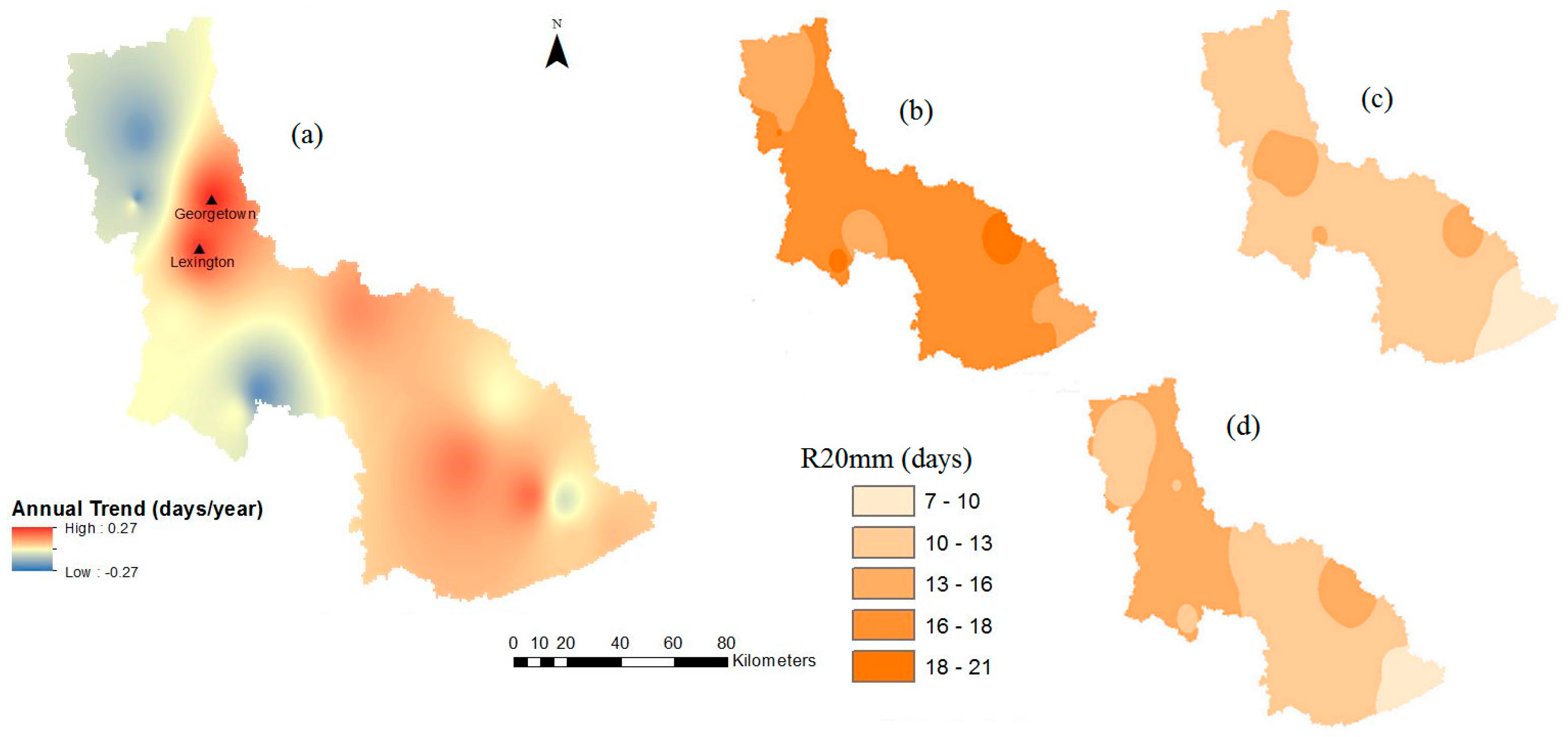
3.5. R20mm
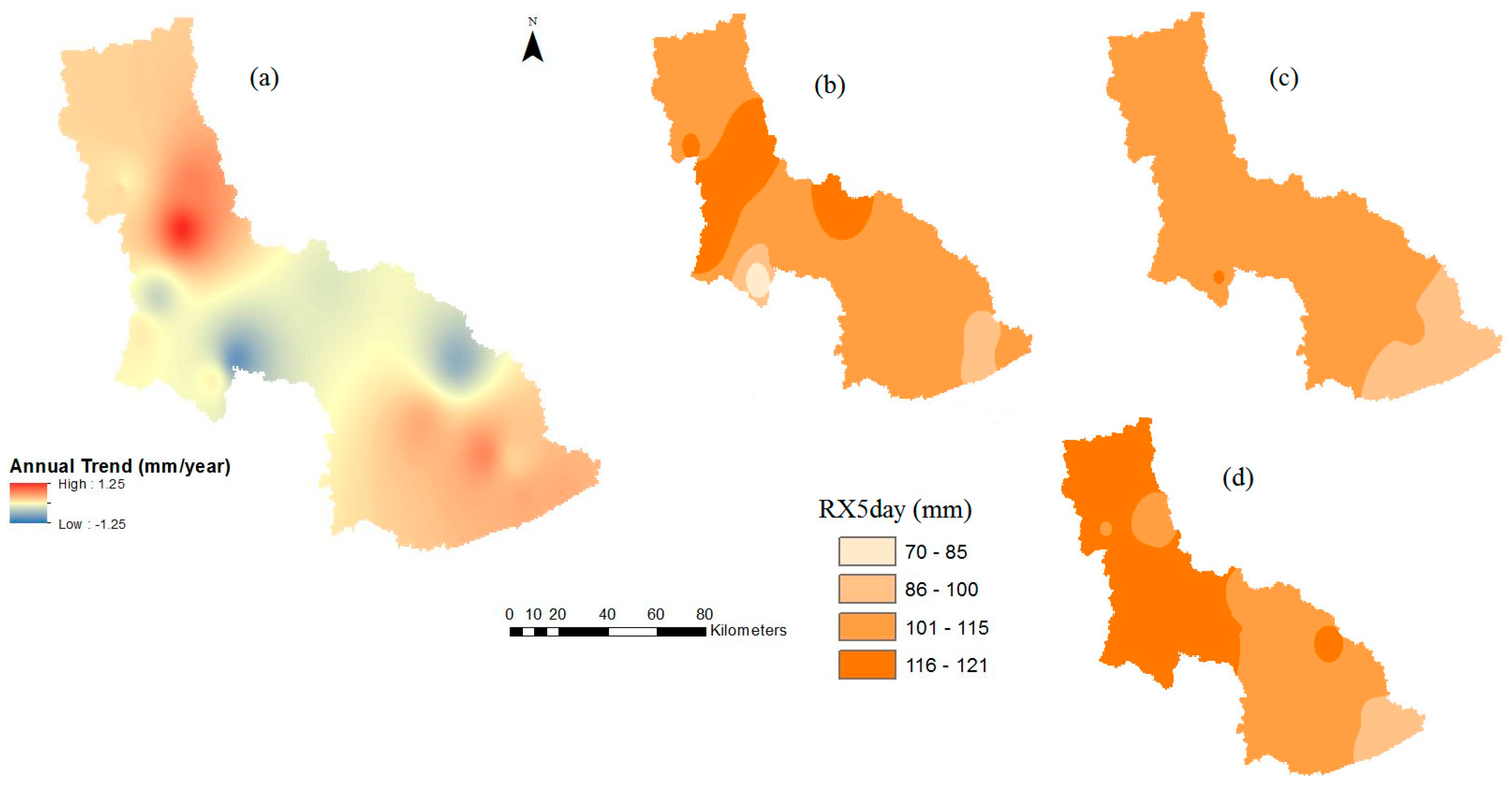
3.6. RX5day
3.7. SDII
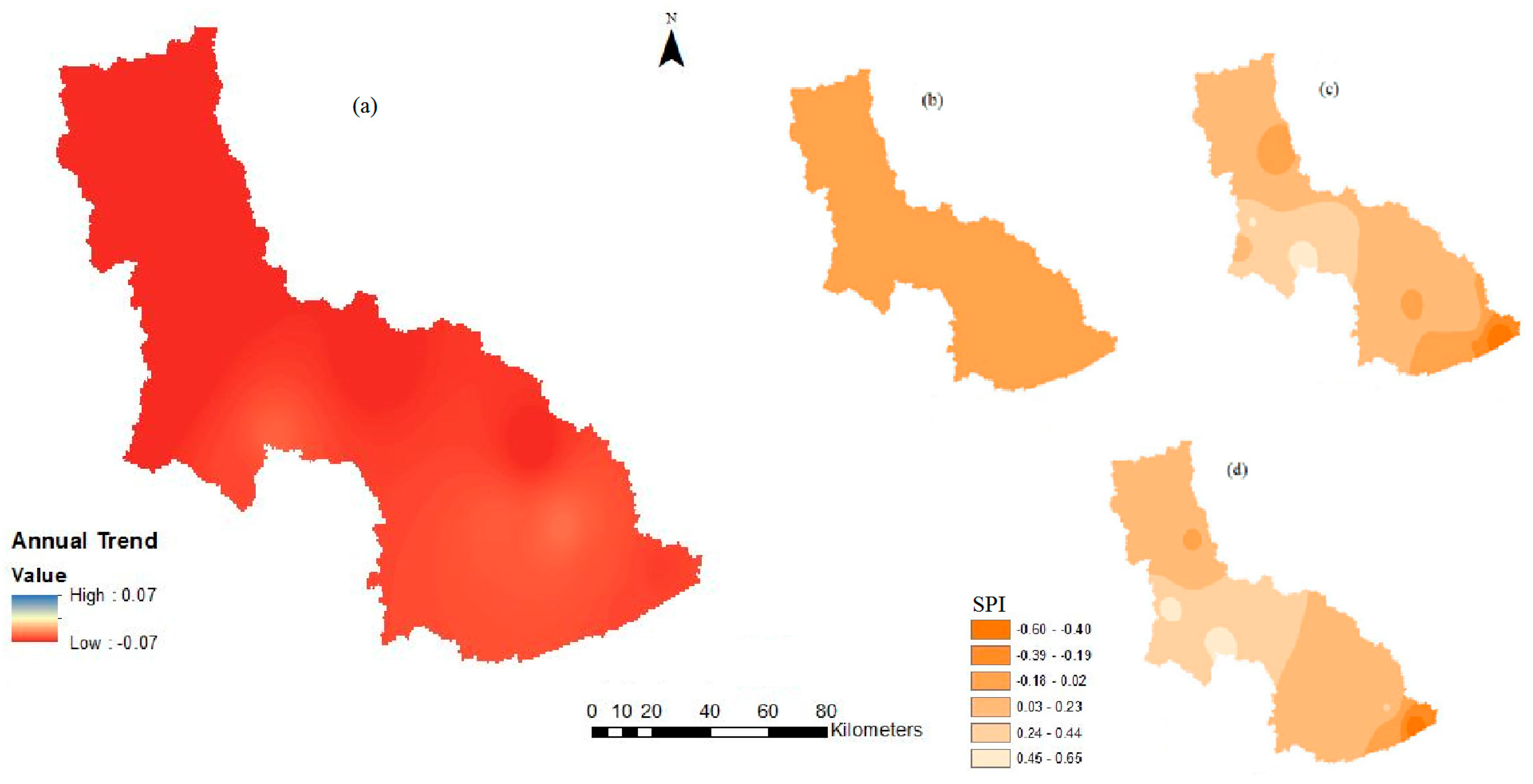
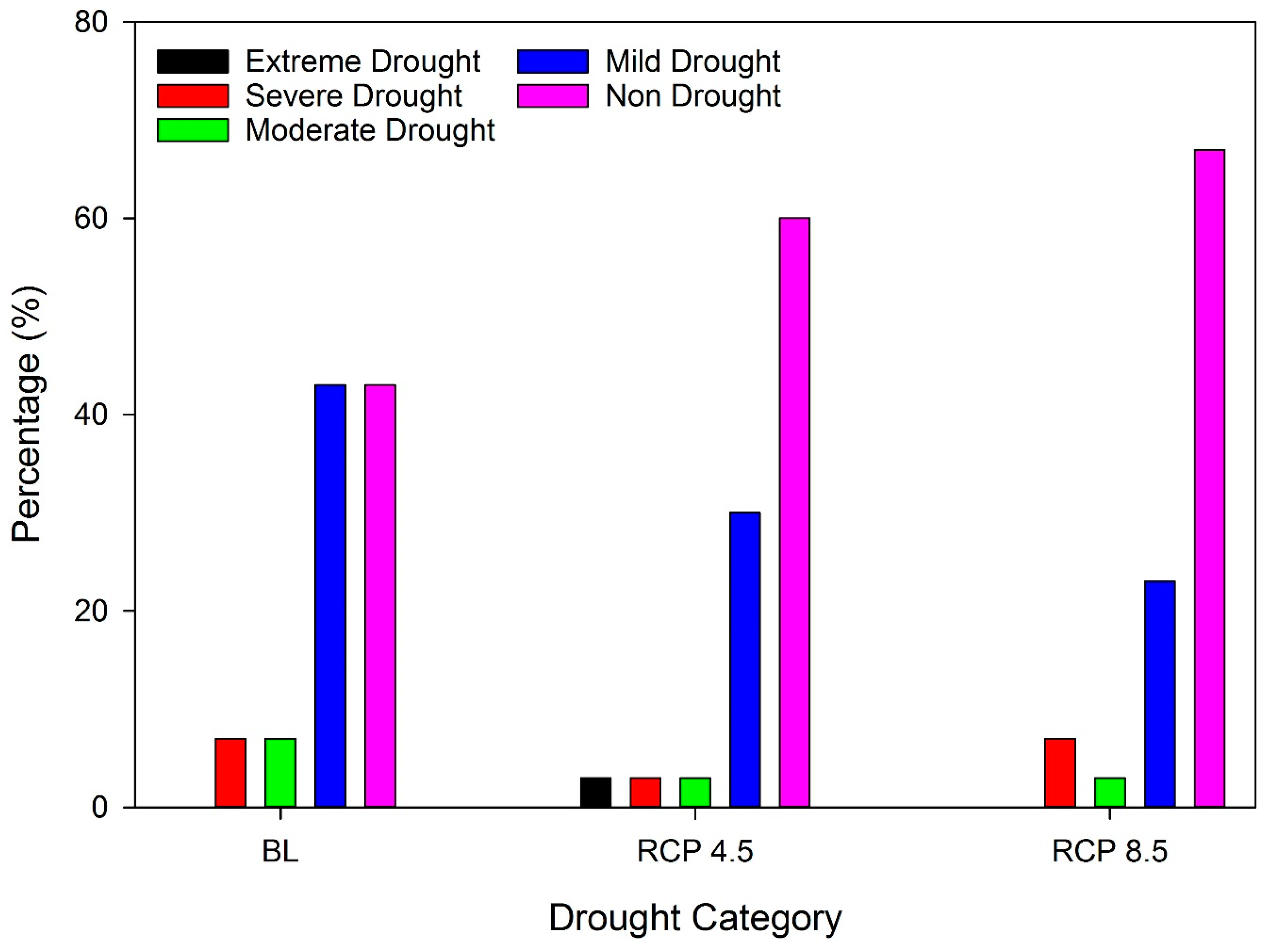
3.8. SPI
4. Summary and Conclusions
Acknowledgments
Author Contributions
Conflicts of Interest
References
- Ficklin, D.L.; Barnhart, B.L. Swat hydrologic model parameter uncertainty and its implications for hydroclimatic projections in snowmelt-dependent watersheds. J. Hydrol. 2014, 519, 2081–2090. [Google Scholar] [CrossRef]
- Chattopadhyay, S.; Jha, M.K. Hydrological response due to projected climate variability in Haw River watershed, North Carolina, USA. Hydrol. Sci. J. 2016, 61, 495–506. [Google Scholar] [CrossRef]
- Narsimlu, B.; Gosain, A.K.; Chahar, B.R. Assessment of future climate change impacts on water resources of upper Sind River basin, India using SWAT model. Water Resour. Manag. 2013, 27, 3647–3662. [Google Scholar] [CrossRef]
- Ashraf, V.S.; Mousavi, S.J.; Abbaspour, K.C.; Srinivasan, R.; Yang, H. Analyses of the impact of climate change on water resources components, drought and wheat yield in semiarid regions: Karkheh River basin in Iran. Hydrol. Process. 2014, 28, 2018–2032. [Google Scholar] [CrossRef]
- Mehan, S.; Kannan, N.; Neupane, R.P.; McDaniel, R.; Kumar, S. Climate change impacts on the hydrological processes of a small agricultural watershed. Climate 2016, 4, 56. [Google Scholar] [CrossRef]
- Intergovernmental Panel on Climate Change. Climate Change 2013: The Physical Science Basis. Contribution of Working Group I to the Fifth Assessment Report of the Intergovernmental Panel on Climate Change; Stocker, T.F., Qin, D., Plattner, G.K., Tignor, M., Allen, S.K., Boschung, J., Nauels, A., Xia, Y., Bex, C., Midgley, P.M., Eds.; Cambridge University Press: Cambridge, UK, 2013; p. 1535. [Google Scholar]
- Hirabayashi, Y.; Mahendran, R.; Koirala, S.; Konoshima, L.; Yamazaki, D.; Watanabe, S.; Kim, H.; Kanae, S. Global flood risk under climate change. Nat. Clim. Chang. 2013, 3, 816–821. [Google Scholar] [CrossRef]
- Portmann, R.W.; Solomon, S.; Hegerl, G.C. Spatial and seasonal patterns in climate change, temperatures, and precipitation across the United States. Proc. Natl. Acad. Sci. USA 2009, 106, 7324–7329. [Google Scholar] [CrossRef] [PubMed]
- Karl, T.R.; Meehl, G.A.; Peterson, T.C. Global Climate Change Impacts in the United States; Cambridge University Press: Cambridge, UK, 2009. [Google Scholar]
- Sayemuzzaman, M.; Jha, M.K. Seasonal and annual precipitation time series trend analysis in North Carolina, United States. Atmos. Res. 2014, 137, 183–194. [Google Scholar] [CrossRef]
- Gao, Y.; Fu, J.S.; Drake, J.B.; Liu, Y.; Lamarque, J.F. Projected changes of extreme weather events in the eastern United States based on a high resolution climate modeling system. Environ. Res. Lett. 2012, 7, 044025. [Google Scholar] [CrossRef]
- Chattopadhyay, S.; Edwards, D. Long-term trend analysis of precipitation and air temperature for Kentucky, United States. Climate 2016, 4, 10. [Google Scholar] [CrossRef]
- Intergovernmental Panel on Climate Change. Managing the Risks of Extreme Events and Disasters to Advance Climate Change Adaptation. A Special Report of Working Groups I and II of the Intergovernmental Panel on Climate Change. Cambridge, 2012. Available online: http://www.ipcc-wg2.gov/SREX/images/uploads/SREX-All_FINAL.pdf (accessed on 14 April 2016). [Google Scholar]
- Ren, Z.; Zhang, M.; Wang, S.; Qiang, F.; Zhu, X.; Dong, L. Changes in daily extreme precipitation events in south China from 1961 to 2011. J. Geogr. Sci. 2015, 25, 58–68. [Google Scholar] [CrossRef]
- De Lima, M.I.P.; Santo, F.E.; Ramos, A.M.; Trigo, R.M. Trends and correlations in annual extreme precipitation indices for mainland Portugal, 1941–2007. Theor. Appl. Climatol. 2015, 119, 55–75. [Google Scholar] [CrossRef]
- Mondal, A.; Mujumdar, P.P. On the detection of human influence in extreme precipitation over India. J. Hydrol. 2015, 529, 1161–1172. [Google Scholar] [CrossRef]
- Kamruzzaman, M.; Beecham, S.; Metcalfe, A.V. Estimation of trends in rainfall extremes with mixed effects models. Atmos. Res. 2016, 168, 24–32. [Google Scholar] [CrossRef]
- Roth, M.; Buishand, T.A.; Jongbloed, G. Trends in moderate rainfall extremes: A regional monotone regression approach. J. Clim. 2015, 28, 8760–8769. [Google Scholar] [CrossRef]
- Yuan, X.; Wood, E.F.; Luo, L.; Pan, M. A first look at climate forecast system version 2 (cfsv2) for hydrological seasonal prediction. Geophys. Res. Lett. 2011, 38, L13402. [Google Scholar] [CrossRef]
- Mearns, L.O.; Lettenmaier, D.P.; McGinnis, S. Uses of results of regional climate model experiments for impacts and adaptation studies: The example of NARCCAP. Curr. Clim. Chang. Rep. 2015, 1, 1–9. [Google Scholar] [CrossRef]
- Fu, G.; Liu, Z.; Charles, S.P.; Xu, Z.; Yao, Z. A score-based method for assessing the performance of gcms: A case study of Southeastern Australia. J. Geophys. Res. Atmos. 2013, 118, 4154–4167. [Google Scholar] [CrossRef]
- Deser, C.; Phillips, A.; Bourdette, V.; Teng, H. Uncertainty in climate change projections: The role of internal variability. Clim. Dyn. 2012, 38, 527–546. [Google Scholar] [CrossRef]
- Rocheta, E.; Sugiyanto, M.; Johnson, F.; Evans, J.; Sharma, A. How well do general circulation models represent low-frequency rainfall variability? Water Resour. Res. 2014, 50, 2108–2123. [Google Scholar] [CrossRef]
- Emori, S.; Hasegawa, A.; Suzuki, T.; Dairaku, K. Validation, parameterization dependence, and future projection of daily precipitation simulated with a high-resolution atmospheric GCM. Geophys. Res. Lett. 2005, 32, 541–544. [Google Scholar] [CrossRef]
- Lafon, T.; Dadson, S.; Buys, G.; Prudhomme, C. Bias correction of daily precipitation simulated by a regional climate model: A comparison of methods. Int. J. Climatol. 2013, 33, 1367–1381. [Google Scholar] [CrossRef] [Green Version]
- Ines, A.V.M.; Hansen, J.W. Bias correction of daily gcm rainfall for crop simulation studies. Agric. For. Meteorol. 2006, 138, 44–53. [Google Scholar] [CrossRef]
- Mahoney, K.; Alexander, M.; Scott, J.D.; Barsugli, J. High-resolution downscaled simulations of warm-season extreme precipitation events in the Colorado front range under past and future climates. J. Clim. 2013, 26, 8671–8689. [Google Scholar] [CrossRef]
- Sunyer, M.A.; Hundecha, Y.; Lawrence, D.; Madsen, H.; Willems, P.; Martinkova, M.; Vormoor, K.; Bürger, G.; Hanel, M.; Kriaučiūnienė, J.; et al. Inter-comparison of statistical downscaling methods for projection of extreme precipitation in Europe. Hydrol. Earth Syst. Sci. 2015, 19, 1827–1847. [Google Scholar] [CrossRef] [Green Version]
- Johnson, F.; Sharma, A. Measurement of gcm skill in predicting variables relevant for hydroclimatological assessments. J. Clim. 2009, 22, 4373–4382. [Google Scholar] [CrossRef]
- Radić, V.; Clarke, G.K.C. Evaluation of ipcc models’ performance in simulating late-twentieth-century climatologies and weather patterns over North America. J. Clim. 2011, 24, 5257–5274. [Google Scholar] [CrossRef]
- Miao, C.; Duan, Q.; Yang, L.; Borthwick, A.G.L. On the applicability of temperature and precipitation data from CMIP3 for China. PLoS ONE 2012, 7, e44659. [Google Scholar] [CrossRef] [PubMed] [Green Version]
- National Drought Mitigation Center. From Too Much to Too Little: How the Central U.S. Drought of 2012 Evolved Out of One of the Most Devastating Floods on Record in 2011. 2012. Available online: http://drought.unl.edu/Portals/0/docs/CentralUSDroughtAssessment2012.pdf (accessed on 17 March 2016).
- Kentucky River Facts. Available online: http://kyriverkeeper.org/kentucky-river-facts/ (accessed on 18 June 2016).
- Pierce, D.W.; Cayan, D.R.; Maurer, E.P.; Abatzoglou, J.T.; Hegewisch, K.C. Improved bias correction techniques for hydrological simulations of climate change. J. Hydrometeorol. 2015, 16, 2421–2442. [Google Scholar] [CrossRef]
- Li, H.; Sheffield, J.; Wood, E.F. Bias correction of monthly precipitation and temperature fields from intergovernmental panel on climate change AR4 models using equidistant quantile matching. J. Geophys. Res. Atmos. 2010, 115, 985–993. [Google Scholar] [CrossRef]
- Schoof, J.T.; Robeson, S.M. Projecting changes in regional temperature and precipitation extremes in the United States. Weather Clim. Extrem. 2016, 11, 28–40. [Google Scholar] [CrossRef]
- Guijarro, J.A. User’s Guide to Climatol. 2013. Available online: http://www.climatol.eu/climatol-guide.pdf (accessed on 8 January 2016).
- Jha, M.K.; Gassman, P.W. Changes in hydrology and streamflow as predicted by a modelling experiment forced with climate models. Hydrol. Process. 2014, 28, 2772–2781. [Google Scholar] [CrossRef]
- Zhang, Y.; Su, F.; Hao, Z.; Xu, C.; Yu, Z.; Wang, L.; Tong, K. Impact of projected climate change on the hydrology in the headwaters of the Yellow River Basin. Hydrol. Process. 2015, 29, 4379–4397. [Google Scholar] [CrossRef]
- Venkataraman, K.; Tummuri, S.; Medina, A.; Perry, J. 21st century drought outlook for major climate divisions of Texas based on CMIP5 multimodel ensemble: Implications for water resource management. J. Hydrol. 2016, 534, 300–316. [Google Scholar] [CrossRef]
- Maurer, E.P.; Adam, J.C.; Wood, A.W. Climate model based consensus on the hydrologic impacts of climate change to the Rio Lempa basin of Central America. Hydrol. Earth Syst. Sci. 2009, 13, 183–194. [Google Scholar] [CrossRef]
- Bennett, K.E.; Werner, A.T.; Schnorbus, M. Uncertainties in hydrologic and climate change impact analyses in headwater basins of British Columbia. J. Clim. 2012, 25, 5711–5730. [Google Scholar] [CrossRef]
- Rana, A.; Moradkhani, H. Spatial, temporal and frequency based climate change assessment in Columbia River basin using multi downscaled-scenarios. Clim. Dyn. 2015, 361–363, 1–22. [Google Scholar] [CrossRef]
- Wood, A.W.; Leung, L.R.; Sridhar, V.; Lettenmaier, D.P. Hydrologic implications of dynamical and statistical approaches to downscaling climate model outputs. Clim. Chang. 2004, 62, 189–216. [Google Scholar] [CrossRef]
- Thrasher, B.; Maurer, E.P.; McKellar, C.; Duffy, P.B. Technical note: Bias correcting climate model simulated daily temperature extremes with quantile mapping. Hydrol. Earth Syst. Sci. 2012, 16, 3309–3314. [Google Scholar] [CrossRef]
- Ning, L.; Riddle, E.E.; Bradley, R.S. Projected changes in climate extremes over the Northeastern United States. J. Clim. 2015, 28, 3289–3310. [Google Scholar] [CrossRef]
- Panofsky, H.A.; Brier, G.W. Some Applications of Statistics to Meteorology; The Pennsylvania State University: University Park, PA, USA, 1968. [Google Scholar]
- Coats, R.; Costa-Cabral, M.; Riverson, J.; Reuter, J.; Sahoo, G.; Schladow, G.; Wolfe, B. Projected 21st century trends in hydroclimatology of the Tahoe Basin. Clim. Chang. 2013, 116, 51–69. [Google Scholar] [CrossRef]
- Lewis, S.C.; Karoly, D.J. Assessment of forced responses of the Australian Community Climate and Earth System Simulator (ACCESS) 1.3 in CMIP5 historical detection and attribution experiments. Aust. Meteorol. Oceanogr. J. 2014, 64, 87–101. [Google Scholar]
- Xiao-Ge, X.; Tong-Wen, W.; Jie, Z. Introduction of CMIP5 experiments carried out with the climate system models of Beijing Climate Center. Adv. Clim. Chang. Res. 2013, 4, 41–49. [Google Scholar] [CrossRef]
- Gent, P.R.; Danabasoglu, G.; Donner, L.J.; Holland, M.M.; Hunke, E.C.; Jayne, S.R.; Lawrence, D.M.; Neale, R.B.; Rasch, P.J.; Vertenstein, M.; et al. The community climate system model version 4. J. Clim. 2011, 24, 4973–4991. [Google Scholar] [CrossRef]
- Voldoire, A.; Sanchez-Gomez, E.; Salas y Mélia, D.; Decharme, B.; Cassou, C.; Sénési, S.; Valcke, S.; Beau, I.; Alias, A.; Chevallier, M.; et al. The CNRMCM5.1 global climate model: Description and basic evaluation. Clim. Dyn. 2013, 40, 2091–2121. [Google Scholar] [CrossRef] [Green Version]
- Donner, L.J.; Wyman, B.L.; Hemler, R.S.; Horowitz, L.W.; Ming, Y.; Zhao, M.; Golaz, J.-C.; Ginoux, P.; Lin, S.-J.; Schwarzkopf, M.D.; et al. The dynamical core, physical parameterizations, and basic simulation characteristics of the atmospheric component AM3 of the GFDL global coupled model CM3. J. Clim. 2011, 24, 3484–3519. [Google Scholar] [CrossRef]
- Jones, C.D.; Hughes, J.K.; Bellouin, N.; Hardiman, S.C.; Jones, G.S.; Knight, J.; Liddicoat, S.; O’Connor, F.M.; Andres, R.J.; Bell, C.; et al. The HADGEM2-AS implementation of CMIP5 centennial simulations. Geosci. Model Dev. 2011, 4, 543–570. [Google Scholar] [CrossRef] [Green Version]
- Dufresne, J.-L.; Foujols, M.-A.; Denvil, S.; Caubel, A.; Marti, O.; Aumont, O.; Balkanski, Y.; Bekki, S.; Bellenger, H.; Benshila, R.; et al. Climate change projections using the IPSL-CM5A earth system model: From CMIP3 to CMIP5. Clim. Dyn. 2013, 40, 2123–2165. [Google Scholar] [CrossRef] [Green Version]
- Watanabe, M.; Suzuki, T.; O’ishi, R.; Komuro, Y.; Watanabe, S.; Emori, S.; Takemura, T.; Chikira, M.; Ogura, T.; Sekiguchi, M.; et al. Improved climate simulation by MIROC5: Mean states, variability, and climate sensitivity. J. Clim. 2010, 23, 6312–6335. [Google Scholar] [CrossRef]
- Bentsen, M.; Bethke, I.; Debernard, J.B.; Iversen, T.; Kirkevåg, A.; Seland, Ø.; Drange, H.; Roelandt, C.; Seierstad, I.A.; Hoose, C.; et al. The Norwegian earth system model, NORESM1-M-Part 1: Description and basic evaluation of the physical climate. Geosci. Model Dev. 2013, 6, 687–720. [Google Scholar] [CrossRef]
- Santos, M.; Fragoso, M. Precipitation variability in northern Portugal: Data homogeneity assessment and trends in extreme precipitation indices. Atmos. Res. 2013, 131, 34–45. [Google Scholar] [CrossRef]
- Tramblay, Y.; El Adlouni, S.; Servat, E. Trends and variability in extreme precipitation indices over Maghreb countries. Nat. Hazards Earth Syst. Sci. 2013, 13, 3235–3248. [Google Scholar] [CrossRef]
- Bronaugh, D. Package ‘climdex.pcic’. 2014. Available online: https://cran.r-project.org/web/packages/climdex.pcic/climdex.pcic.pdf (accessed on 17 February 2016).
- McKee, T.; Doesken, N.; Kleist, J. The relationship of drought frequency and duration to time scales. In Proceedings of the 8th Conference on Applied Climatology, Anaheim, CA, USA, January 17–22 1993.
- Chen, T.; Werf, G.R.; Jeu, R.A.M.; Wang, G.; Dolman, A.J. A global analysis of the impact of drought on net primary productivity. Hydrol. Earth Syst. Sci. 2013, 17, 3885–3894. [Google Scholar] [CrossRef]
- Wang, Q.; Wu, J.; Lei, T.; He, B.; Wu, Z.; Liu, M.; Mo, X.; Geng, G.; Li, X.; Zhou, H.; et al. Temporal-spatial characteristics of severe drought events and their impact on agriculture on a global scale. Quat. Int. 2014, 349, 10–21. [Google Scholar] [CrossRef]
- Neves, J. Package ‘spi’. Available online: https://cran.r-project.org/web/packages/spi/spi.pdf (accessed on 5 April 2016).
- Kendall, S. Time Series; Oxford University Press: New York, NY, USA, 1976. [Google Scholar]
- Xu, W.; Zou, Y.; Zhang, G.; Linderman, M. A comparison among spatial interpolation techniques for daily rainfall data in Sichuan Province, China. Int. J. Climatol. 2015, 35, 2898–2907. [Google Scholar] [CrossRef]
- Taylor, K.E. Summarizing multiple aspects of model performance in a single diagram. J. Geophys. Res. Atmos. 2001, 106, 7183–7192. [Google Scholar] [CrossRef]
- Taye, M.T.; Ntegeka, V.; Ogiramoi, N.P.; Willems, P. Assesment of climate change impact on hydrological extremes in two source regions of the Nile River Basin. Hydrol. Earth Syst. Sci. 2011, 15, 209–222. [Google Scholar] [CrossRef] [Green Version]
- Schoof, J.T. High-resolution projections of 21st century daily precipitation for the contiguous U.S. J. Geophys. Res. Atmos. 2015, 120, 3029–3042. [Google Scholar] [CrossRef]
- Mishra, V.; Lettenmaier, D.P. Climatic trends in major U.S. urban areas, 1950–2009. Geophys. Res. Lett. 2011, 38, 136. [Google Scholar] [CrossRef]
- Zilli, M.T.; Carvalho, L.M.V.; Liebmann, B.; Silva Dias, M.A. A comprehensive analysis of trends in extreme precipitation over southeastern coast of Brazil. Int. J. Climatol. 2016. [Google Scholar] [CrossRef]
- Lovejoy, S. What is climate? Eos Trans. Am. Geophys. Union 2013, 94, 1–2. [Google Scholar] [CrossRef]


| Station Name | Latitude (° N) | Longitude (° W) | Elevation (m) | Mean Annual Rainfall (mm) | Missing Data |
|---|---|---|---|---|---|
| Whitesburg | 37.1167 | −82.8167 | 355.1 | 1308.0 ± 184.5 | 1% |
| Skyline | 37.0667 | −82.9667 | 366.1 | 1233.0 ± 197.3 | <1% |
| Carr Fork | 37.2333 | −83.0333 | 309.1 | 1159.9 ± 226.1 | <1% |
| Hazard | 37.2500 | −83.1833 | 267.9 | 1287.5 ± 219.1 | <1% |
| Buckhorn | 37.3500 | −83.3833 | 285.3 | 1266.7 ± 214.7 | <1% |
| Jackson | 37.6000 | −83.3167 | 416.1 | 1273.9 ± 213.1 | <1% |
| Crab Orchard | 37.4833 | −84.4333 | 335.9 | 1238.0 ± 199.2 | <1% |
| Berea | 37.5666 | −84.3333 | 309.1 | 1201.0 ± 192.8 | <1% |
| Danville | 37.6500 | −84.7667 | 291.1 | 1228.4 ± 247.1 | <1% |
| Dix Dam | 37.8000 | −84.7167 | 265.2 | 1116.4 ± 251.3 | 1% |
| Clay | 37.8666 | −83.9333 | 192.0 | 1172.0 ± 242.7 | <1% |
| Lexington | 38.0333 | −84.6000 | 294.4 | 1220.6 ± 227.3 | <1% |
| Frankfort Lock | 38.2333 | −84.8667 | 152.4 | 1176.2 ± 203.6 | 2% |
| Frankfort | 38.1833 | −84.9000 | 230.1 | 1249.0 ± 250.9 | <1% |
| Georgetown | 38.2000 | −84.5500 | 271.0 | 1224.2 ± 233.8 | <1% |
| Gest Lock | 38.4167 | −84.8833 | 149.4 | 1153.6 ± 201.0 | 1% |
| Model Name | Institution | Spatial Resolution | Reference |
|---|---|---|---|
| ACCESS 1-0 | Commonwealth Scientific and Industrial Research Organization, Australia | 1.9° × 1.2° | Lewis and Karoly [49] |
| BCC-CSM 1.1 | Beijing Climate Center, China Meteorological Administration, China | 2.8° × 2.8° | Xin et al. [50] |
| CCSM4 | National Center for Atmospheric Research, United States | 1.25° × 0.94° | Gent et al. [51] |
| CNRM-CM5 | National Center for Meteorological Research, France | 1.4° × 1.4° | Voldoire et al. [52] |
| GFDL-ESM2G | NOAA/Geophysical Fluid Dynamics Laboratory, United States | 2.5° × 2.0° | Donner et al. [53] |
| HadGEM2-CC | Met Office Hadley Center, United Kingdom | 1.9° × 1.2° | Jones et al. [54] |
| IPSL-CM5A-MR | L’Institut Pierre-Simon Laplace, France | 2.5° × 1.25° | Dufresne et al. [55] |
| MIROC5 | Japan Agency for Marine-Earth Sciences and Technology, Atmosphere and Ocean Research and National Institute for Environmental Studies, Japan | 1.4° × 1.4° | Watanabe et al. [56] |
| MIROC-ESM | Japan Agency for Marine-Earth Sciences and Technology, Atmosphere and Ocean Research and National Institute for Environmental Studies, Japan | 2.8° × 2.8° | Watanabe et al. [56] |
| NorESM1-M | Norwegian Climate Center, Norway | 2.5° × 1.8° | Bentsen et al. [57] |
| Level | Drought Category | SPI Values |
|---|---|---|
| 0 | Non-drought | 0 ≤ SPI |
| 1 | Mild drought | −1.0 < SPI < 0 |
| 2 | Moderate drought | −1.5 < SPI < −1.0 |
| 3 | Severe drought | −2.0 < SPI < −1.5 |
| 4 | Extreme drought | SPI ≤ −2.0 |
| Model | MAE (mm) | NSD (mm) |
|---|---|---|
| ACCESS 1-0 | 206.65 | 0.97 |
| BCC-CSM 1.1 | 164.51 | 0.84 |
| CCSM4 | 202.35 | 0.92 |
| CNRM-CM5 | 177.12 | 1.18 |
| GFDL-ESM2G | 136.21 | 1.02 |
| HadGEM2-CC | 140.58 | 0.78 |
| IPSL-CM5A-MR | 203.89 | 0.70 |
| MIROC5 | 169.37 | 0.98 |
| MIROC-ESM | 206.87 | 0.92 |
| NorESM1-M | 164.67 | 0.69 |
| Ensemble Mean | 134.73 | 0.27 |
| Stations | PRCPTOT (mm) | CDD (Days) | CWD (Days) | R20mm (Days) | RX5day (mm) | SDII (mm/Day) | SPI |
|---|---|---|---|---|---|---|---|
| Trend (mm/Year) | Trend (Days/Year) | Trend (Days/Year) | Trend (Days/Year) | Trend (mm/Year) | Trend (mm/Day/Year) | Trend (SPI Value/Year) | |
| Whitesburg | |||||||
| Mean | 1284 ± 185 | 13.5 ± 3.3 | 9.6 ± 2.6 | 14.0 ± 4.3 | 101 ± 25 | 8.0 ± 1.2 | 0.0 ± 1.2 |
| Trend | −0.97 | −0.04 | 0.00 | 0.08 | 0.50 | 0.04 | −0.01 |
| Skyline | |||||||
| Mean | 1221 ± 197 | 15 ± 4 | 6.0 ± 1.5 | 16.6 ± 4.5 | 97 ± 24 | 9.8 ± 1.1 | 0.0 ± 1.1 |
| Trend | 4.50 | −0.09 | 0.03 | 0.05 | 0.51 | 0.00 | −0.02 |
| Carr Fork | |||||||
| Mean | 1143 ± 225 | 17.1 ± 4.7 | 5.9 ± 2.1 | 14.8 ± 5.6 | 95 ± 29 | 9.6 ± 1.6 | 0.0 ± 1.2 |
| Trend | 0.22 | 0.00 | 0.00 | −0.05 | 0.25 | −0.02 | −0.00 |
| Hazard | |||||||
| Mean | 1278 ± 221 | 16.7 ± 3.9 | 5.9 ± 1.3 | 18.4 ± 5.1 | 111 ± 35 | 10.7 ± 1.3 | 0.0 ± 1 |
| Trend | 7.78 | 0.00 | 0.00 | 0.18 | 0.71 | 0.04 | −0.02 |
| Buckhorn | |||||||
| Mean | 1249 ± 217 | 16.4 ± 4.3 | 7.6 ± 2.6 | 15.6 ± 6.7 | 101 ± 23 | 9.2 ± 1.7 | 0.0 ± 1.1 |
| Trend | 7.92 | −0.04 | 0.00 | 0.17 | 0.50 | 0.04 | −0.01 |
| Jackson | |||||||
| Mean | 1260 ± 213 | 16.3 ± 4.5 | 5.9 ± 2.0 | 18.9 ± 6.0 | 112 ± 27 | 10.7 ± 1.5 | 0.0 ± 1.1 |
| Trend | 2.30 | 0.00 | 0.00 | 0.00 | −0.70 | 0.00 | −0.01 |
| Crab Orchard | |||||||
| Mean | 1230 ± 199 | 19.4 ± 5.4 | 6.0 ± 1.8 | 19.4 ± 4.8 | 72 ± 41 | 11.8 ± 1.8 | 0.0 ± 1.3 |
| Trend | 6.81 | 0.00 | 0.04 | 0.00 | 0.08 | 0.05 | −0.00 |
| Berea | |||||||
| Mean | 1182 ± 194 | 15.2 ± 3.0 | 8.4 ± 2.4 | 13.4 ± 6.3 | 105 ± 30 | 8.8 ± 2.2 | 0.0 ± 1.2 |
| Trend | 2.51 | 0.04 | 0.08 | −0.21 | −0.94 | −0.06 | −0.01 |
| Danville | |||||||
| Mean | 1217 ± 246 | 19.0 ± 5.7 | 5.4 ± 1.6 | 18.4 ± 5.0 | 123 ± 42 | 11.8 ± 1.9 | 0.0 ± 1.2 |
| Trend | 2.08 | 0.13 | 0.00 | 0.00 | 0.10 | −0.03 | −0.02 |
| Dix Dam | |||||||
| Mean | 1107 ± 250 | 20.6 ± 7.6 | 5.7 ± 1.6 | 16.2 ± 4.8 | 118 ± 39 | 11.05 ± 1.6 | 0.0 ± 1.2 |
| Trend | −0.21 | 0.16 | 0.00 | 0.00 | −0.35 | −0.01 | −0.02 |
| Clay | |||||||
| Mean | 1169 ± 242 | 21.6 ± 8.0 | 5.1 ± 1.7 | 18.4 ± 5.3 | 122 ± 38 | 13.5 ± 2.9 | 0.0 ± 1.1 |
| Trend | 15.68 | −0.34 | 0.14 | 0.14 | −0.21 | −0.20 | −0.00 |
| Lexington | |||||||
| Mean | 1208 ± 227 | 17.7 ± 4.3 | 5.1 ± 1.1 | 18.2 ± 5.2 | 122 ± 35 | 11.6 ± 1.4 | 0.0 ± 1.2 |
| Trend | 10.63 | 0.00 | 0.00 | 0.25 | 1.25 | 0.07 | −0.07 |
| Frankfort Lock | |||||||
| Mean | 1156 ± 202 | 16.7 ± 3.3 | 6.8 ± 2.5 | 14.4 ± 5.8 | 107 ± 29 | 9.9 ± 2.3 | 0.0 ± 1.2 |
| Trend | 7.54 | −0.10 | 0.15 | −0.20 | 0.03 | −0.16 | −0.01 |
| Frankfort | |||||||
| Mean | 1239 ± 248 | 18.6 ± 5.3 | 6.0 ± 1.7 | 18.9 ± 5.0 | 120 ± 41 | 11.8 ± 1.4 | 0.0 ± 1.2 |
| Trend | 1.34 | −0.10 | 0.00 | 0.00 | 0.25 | −0.02 | −0.00 |
| Georgetown | |||||||
| Mean | 1212 ± 232 | 16.6 ± 4.4 | 6.3 ± 2.0 | 17.7 ± 5.6 | 116 ± 38 | 10.8 ± 1.7 | 0.0 ± 1.2 |
| Trend | 12.51 | −0.09 | 0.00 | 0.27 | 0.74 | 0.07 | −0.01 |
| Gest Lock | |||||||
| Mean | 1139 ± 199 | 18.2 ± 7.0 | 6.9 ± 2.4 | 14.1 ± 5.7 | 109 ± 39 | 9.8 ± 2.5 | 0.0 ± 1.2 |
| Trend | 7.62 | −0.05 | 0.12 | −0.18 | 0.27 | −0.12 | −0.03 |
| Overall | |||||||
| Mean | 1206 ± 52 | 17.4 ± 2.1 | 6.4 ± 1.2 | 16.7 ± 2.1 | 108 ± 13 | 10.6 ± 1.4 | 0.0 ± 0.92 |
| Trend | 5.51 | −0.03 | 0.03 | 0.03 | 0.19 | −0.02 | −0.02 |
© 2017 by the authors. Licensee MDPI, Basel, Switzerland. This article is an open access article distributed under the terms and conditions of the Creative Commons Attribution (CC BY) license ( http://creativecommons.org/licenses/by/4.0/).
Share and Cite
Chattopadhyay, S.; Edwards, D.R.; Yu, Y. Contemporary and Future Characteristics of Precipitation Indices in the Kentucky River Basin. Water 2017, 9, 109. https://doi.org/10.3390/w9020109
Chattopadhyay S, Edwards DR, Yu Y. Contemporary and Future Characteristics of Precipitation Indices in the Kentucky River Basin. Water. 2017; 9(2):109. https://doi.org/10.3390/w9020109
Chicago/Turabian StyleChattopadhyay, Somsubhra, Dwayne R. Edwards, and Yao Yu. 2017. "Contemporary and Future Characteristics of Precipitation Indices in the Kentucky River Basin" Water 9, no. 2: 109. https://doi.org/10.3390/w9020109