Applying SHETRAN in a Tropical West African Catchment (Dano, Burkina Faso)—Calibration, Validation, Uncertainty Assessment

Abstract

This study presents the calibration and validation of the physically based spatially distributed hydrological and soil erosion model SHETRAN for the Dano catchment, Burkina Faso. A sensitivity analysis of six model parameters was performed to assess the model response and to reduce the number of parameters for calibration. The hydrological component was calibrated and validated using observed discharge data of two years. Statistical quality measures (R², NSE, KGE) ranged from 0.79 to 0.66 during calibration and validation. The calibrated hydrological component was used to feed the erosion modeling. The simulated suspended sediment load (SSL) was compared with turbidity-based measurements of SSL of two years. Achieved quality measures are comparable to other SHETRAN studies. Uncertainties of measured discharge and suspended sediment concentration were determined to assess the propagated uncertainty of SSL. The comparison of measurement uncertainties of discharge and SSL with parameter uncertainty of the corresponding model output showed that simulated discharge and SSL were frequently outside the large measured uncertainty bands. A modified NSE was used to incorporate measurement and parameter uncertainty into the efficiency evaluation of the model. The analyses of simulated erosion sources and spatial patterns showed the importance of river erosion contributing more than 60% to the total simulated sediment loss.

1. Introduction

Soil degradation by water-related soil erosion is a major environmental problem threatening food security, income, and environmental health especially in tropical and subtropical countries [1,2,3,4]. On the one hand, systemic and natural reasons such as unfavorable climatic conditions and the structural instability of soils resulting from low soil organic carbon (SOC) content are responsible for a high erosion risk in these regions [1]. On the other hand, socio-economic factors contribute to the problem and are often responsible for the severity of soil erosion. Among those factors, increased pressure on land resources through population growth is highlighted as a major reason for accelerated soil erosion [4,5,6,7].

Soil erosion strongly varies in space and time. Thus measuring soil erosion requires a large personnel and financial effort and despite advances in measurement technology it is often impossible to perform measurements over the required spatial and temporal scales. This especially applies to data scarce regions such as West Africa. To overcome these drawbacks soil erosion models have been frequently used [8,9]. Erosion models have also been implemented to predict the effect of land use and climate change on soil erosion and to identify areas where erosion control measures are necessary [9]. In general, three types of erosion models are differentiated: Empirical erosion models, conceptual models, and physically based erosion models. Physically based erosion models are based on physical principles such as the conservation of mass and momentum [10]. After an evaluation of the available erosion models the physically based spatially distributed soil erosion model SHETRAN [11] was chosen to simulate hydrological and soil erosion processes in a tropical West African catchment. The two main reasons for using SHETRAN in this study are its ability to simulate the dominant erosion processes [12,13] and the continuity in simulation necessary for the prediction of land use and climate change. The study considers soil erosion by surface runoff.

Physically based models, such as SHETRAN, need to be calibrated and validated. Although parameters of physically based models theoretically do not need calibration, adjustments are necessary to account for an unrealistic representation of environmental properties such as grid size or channel geometry. In the present context, calibration is therefore considered as the adjustment of parameter values to overcome the unrealistic representation of environmental properties. The calibration process requires knowledge on the sensitivity of results to model parameters (i) to better assess the model response; (ii) to reduce the number of parameters for calibration; and (iii) to define the parameter uncertainty [14,15]. Outputs of environmental models are subject to uncertainty that is related to the simplification of the model, the uncertainty of the model parameter, and the measurement uncertainty [8,16,17]. Measurement uncertainty refers to the uncertainty of measured data used as input (e.g., precipitation) and to calibrate and validate the model. Studying the uncertainty associated with the modeling output is important since decision making is often based on the output of environmental models [18]. The present study focuses on the assessment of two sources of uncertainty in environmental modeling, the parameter and the measurement uncertainty. Information on and measurements of the required model parameters are difficult if possible at all and often not available for the study area or on the required spatial or temporal scale. Quantifying parameter uncertainty is necessary for the interpretation of model outcomes and its application in environmental planning [9,15].

Measured variables, such as water discharge and suspended sediment concentration (SSC), are subject to uncertainties. These uncertainties are propagated if different measurements are combined to calculate variables that are used to calibrate and validate the model [18,19,20,21]. For instance, the suspended sediment load (SSL), which is frequently used to validate erosion models, is calculated using the SSC and water discharge. Defining ranges of measured uncertainties is important to contextualize the simulated output.

Studies on soil erosion in West Africa often use USLE-based modelling approaches since data required to run and validate complex, physically based and spatially distributed hydrological soil erosion models are rarely available (see

Table 1. Selected studies on soil erosion modelling in West Africa. NSE is the Nash-Sutcliff efficiency.

Study	Model	Location	Spatial/Temporal Resolution	Catchment/Plot Size	Performance
					Discharge	Sediment Yield
Kusimi et al. [22]	RUSLE	Ghana	30 m/annual	23,188 km2	-	-
Bossa et al. [23]	SWAT	Benin	90 m, 250 m/daily (continuous)	6980 km2	0.6 ≤ NSE ≤ 0.9	0.6 ≤ NSE ≤ 0.64
Obeta and Adewumi [24]	WEPP/EUROSEM	Nigeria	-	24 m2	-	-
Schmengler [25]	WEPP	Burkina Faso	-	-	-	-
Schmengler [25]	WATEM	Burkina Faso	20 m/annual	7.9–23.6 km2	-	-
Hiepe [26]	SWAT	Benin	90 m/daily, weekly (continuous)	586–2324 km2	0.81 ≤ NSE ≤ 0.85	0.68 ≤ NSE ≤ 0.7
Visser et al. [27]	EUROSEM	Burkina Faso	-	1 m2, 20 m2	0.7 ≤ R2 ≤ 0.9	-
Karambiri and Ribolzi [28]	KINEROS2	Burkina Faso	-	0.014 km2	-	-
Mati and Veihe [29]	USLE	Ghana	-	900 km2	-	-
Igwe and Mbagwu [30]	SLEMSA	Nigeria	13 km2	17,500 km2	-	-
Roose [31]	USLE	West Africa	-	100–500 m2	-	-

). Empirically based erosion models are relatively easy to use and only a few input data sets are required to run these models. However, their process representation and applicability to complex conditions of land use and climate change is limited [9]. Most of the studies listed in Table 1 are not comparable with the present study since they use different modeling approaches regarding catchment size, continuity, and considered output. Despite numerous studies that applied SHETRAN in different regions and with multiple objectives (see

Table 2. Selected studies using SHETRAN for water flow and/or sediment flow simulations.

Study	Location	Spatial/Temporal Resolution	Catchment/Plot Size	Performance
				Discharge	Sediment Yield
Present study	Burkina Faso	200 m/h (continuous)	126 km2	0.65 ≤ NSE ≤ 0.7	0.2 ≤ NSE ≤ 0.4
Ðukic and Radic [14,32]	Serbia	25 m/h (event)	114 km2	0.8 ≤ R2 ≤ 0.9
Zhang [33]	Portugal	2 km/h (event)	705 km2	0.7 ≤ NSE ≤ 0.8	NSE = 0.56
Mourato et al. [34]	Portugal	-/daily (continuous)	61–834 km2	0.5 ≤ NSE ≤0.7	-
Naseela et al. [35]	India	-/daily (continuous)	69,425 km2	0.8 ≤ R2 ≤0.9	-
Birkinshaw [36]	UK	50 m/h (continuous)	1.5 km2	0.8 ≤ NSE ≤ 0.9	-
Tripkovic [37]	UK	10 m,100 m/h (continuous, event)	0.09 km2, 9.2 km2	0.5 ≤ NSE ≤ 0.9	-
Elliott et al. [38]	New Zealand	20 m/15 min (event)	1.46–167 km2	0.6 ≤ NSE ≤ 0.9	−2.1 ≥ NSE ≤ 0.8
Bathurst et al. [39]	Middle/South America	50–500 m/h, daily (continuous)	0.35–131 km2	0.8 ≤ NSE ≤ 0.9	-
Birkinshaw et al. [40]	Chile	50 m/h (continuous)	0.35 km2	0.8 ≤ NSE ≤ 0.9
de Figueiredo and Bathurst [41]	Brazil	5 m–2 km/daily–monthly (continuous)	100 m2–137 km2	0.3 ≤ R² ≤ 0.9	0.34 ≤ R2 ≤ 0.98
Adams et al. [42]	New Zealand	0.5 m/min (event)	970 m2	0.9	-
Norouzi Banis et al. [43]	UK	20 m/5 min (continuous)	0.03, 0.05 km2	-	-
Anderton et al. [44]	Spain	100 m/20 min (continuous)	0.56 km2, 4.17 km2	0.5 ≤ NSE ≤ 0.9	-
Lukey et al. [45]	France	50 m/daily (continuous)	0.86 km2	0.03 ≤ R² ≤ 0.4	-

) the model has not been tested in the West African environment. The environmental properties of the study catchment such as the low slope angles and the peculiar rainfall pattern may provide a new challenge to SHETRAN. Therefore, the present study may also serve as a model test of the particular environmental conditions found in the study region. Furthermore, the present study can also be considered as an independent check on the ease of use of the model as most of the studies that used SHETRAN before were conducted by members of the team that developed the model. Thus, this study aims to:

(1)

assess the uncertainty of measured discharge and SSL used to calibrate and validate the hydrological and erosion components of SHETRAN;

(2)

perform a detailed sensitivity analysis to define parameter ranges and to reduce the number of calibration parameters;

(3)

use a Latin Hypercube Sampling approach to calibrate the model and to define uncertainty bounds of simulated discharge and SSL;

(4)

evaluate model performance considering the uncertainty of measured data used to compare the model output and parameter uncertainty.

2. Materials and Methods

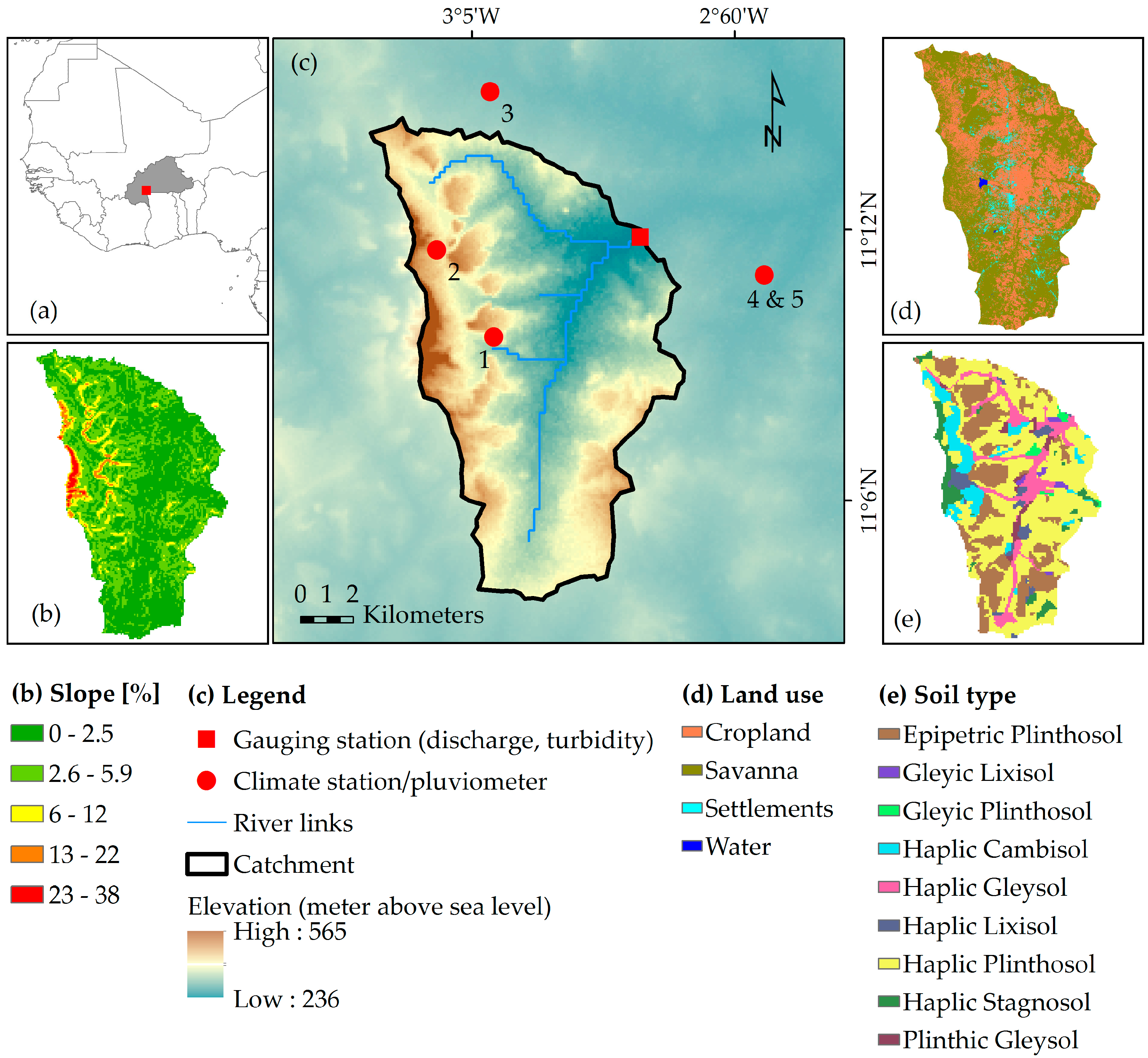
2.1. Study Area

The investigated Dano catchment in the Ioba province covers an area of 126 km² and is located in the Southwest of Burkina Faso (Figure 1). The study area is in a focal watershed of the WASCAL program (West African Science Service Center on Climate Change and Adapted Land Use). The multidisciplinary program is designed to study the influence of climate and land use/land cover change on human and environmental systems and to enhance their resilience.

Agricultural land use is the most important land use category in the region (Figure 1d). The agricultural area has expanded in recent decades due to a growing demographic pressure indicated by an annual population growth of 3%. It has gradually been intensified accompanied by reduced fallow periods and expansion to marginal land areas with adverse effects on soil fertility [4,46,47,48,49]. Since 1990 each year on average 2% of the savanna in the study area was converted to agricultural land [49]. The general appearance of the vegetation in the Sudano savannah is dominated by open forests and wide arborous and shrubby areas. The main staple food crops cultivated in the region are sorghum (Sorghum bicolor), millet (Pennisetum glaucum), maize (Zea mays), cowpeas (Vigna unguiculata), and groundnut (Arachidis hypogaea). Cotton (Gossypium hirsutum) is the most important cash crop. During the rainy season between 40% and 70% of the soil is covered by vegetation.

The catchment is dominated by a flat and slightly undulating landscape characterized by low slope gradients (average and maximum gradients are 3.1% and 38%, respectively, Figure 1b) and an elevation ranging from 236 to 565 m above sea level (m a.s.l). The annual mean temperature is 28.6 °C and annual precipitation ranges from 800 to 1200 mm/a for the period 1951–2005 [50]. The rainfall pattern is uni-modal and characterized by a distinct rainy season from May to October and a dry season from November to April. Eighty percent of the rain falls between July and September with high rainfall intensities. As an example from the Dano catchment, 60 mm/h were measured as maximum in 2014. The flow regime is ephemeral and the channel geometry is divers ranging from strongly incised (3–4 m) clearly defined channels to broader inland valleys. Information on the ranges of measured parameters is given in

Table 3. Range of the measured parameters for the years 2014 and 2015. SSC refers to suspended sediment concentration and SSL to suspended sediment load.

Parameter	Station Number	Measured Range
		2014	2015
Rainfall (mm/h)	1	0–25	0–48.6
	2	0–40.4	0–51.5
	3	0–60.1	0–46
	4	0–42.8	0–37.7
	5	0–43.1	0–35.2
Average daily discharge (m3/s)		0–16.8	0–26.2
Average daily SSC (kg/m3)		0.01–0.3	0.009–0.47
Average daily SSL (kg/s)		0.001–1.9	0.001–4.7

.

Most of the soils (73%) are plinthosols according to the World Reference Base for soil resources (WRB) [51] characterized by a high content of coarse particles and a plinthitic subsurface layer in the first meter of the profile. Other soils that were formed in the region are gleysols, cambisols, lixisols, leptosols, and stagnosols (Figure 1e).

2.2. Data Sources

In order to calibrate and validate SHETRAN, multiple data sets are required (

Table 4. Applied datasets and required inputs for SHETRAN.

Data Set	Resolution/Time Scale	Source	Required Parameters
Topography	90 m	SRTM [52]
Soil	1:25 000	Soil survey	Soil hydrological parameters (α, n 1, Ksat 2, θsat 3, θres 4) texture etc.
Land use map	5 to 250 m	Forkuor [53]	Land use type distribution
Land use characteristic		Literature	LAI 5, Strickler coefficient, ETa/ETp ratio 6
Climate	Hourly, Daily	Instrumentation WASCAL	Rainfall, temperature, humidity, solar radiation, wind speed
Discharge	Hourly	Instrumentation WASCAL	Discharge
Erosion	Hourly, Event	Instrumentation WASCAL	Suspended sediment load, soil erosion rate

Notes: ¹ α and n are van Genuchten empirical parameters; ² K_sat refers to the saturated hydraulic conductivity; ³ θ_sat to the saturated water content; ⁴ θ_res to the residual water content; ⁵ LAI to the leaf area index; and ⁶ ETp/ETa ratio to the ratio of potential evapotranspiration to actual evapotranspiration.

). Existing data were complemented by a measurement network consisting of five automatic climate stations and pluviometers (tipping bucket type) and one discharge and turbidity station. Additionally, physical and chemical analyses of soil samples were done to retrieve necessary soil parameters for the erosion model (Table 4).

2.3. Model Description

Modeling of hydrological and erosion processes was performed using the physically based, spatially distributed and raster-based model SHETRAN [11,12]. SHETRAN is based on SHE (Système Hydrologique Europeen) which was jointly developed by the British Institute of Hydrology, the Danish Hydraulic Institute and the French consulting company SOGREAH [54]. During the last thirty years SHETRAN has been continuously improved and equipped with new components that include e.g., the sediment component [12,55] and a fully 3D subsurface water flow component [56]. A summary of SHETRAN applications with various objectives and in different regions is given in Table 2.

Detailed information about the model is given in Bathurst [57]. A short overview of the most important hydrological process descriptions of the model is summarized in the following list:

• Fully 3D subsurface flow simulation based on Richards’ equation.
• Infiltration is calculated using Richards’ equation.
• Overland and channel flow is calculated using the diffusive wave approximations of the full Saint-Venant equation.
• Potential evapotranspiration (ETp): Potential plant transpiration, evaporation from intercepting surfaces and from bare soil as well as water bodies was calculated externally based on the Penman-Monteith equation [58] and added as input into SHETRAN.
• Actual evapotranspiration (ETa) is estimated based on the approach introduced by Feddes et al. [59] where the ratio ETa/ETp is a function of soil moisture tension. The ratio ETa/ETp at field capacity is the input parameter and the reduction of ETa with decreasing soil moisture tension is calculated based on this parameter.
• Interception is calculated based on the approach by Rutter et al. [60,61] who relates interception to the leaf area index, the vegetation cover, and the maximum depth of water on leaves.

The parameterization and calibration of land use and soil properties was done based on data obtained from literature and measurements (see Table 4 and

Table 5. Soil, land use and erosion parameters in SHETRAN.

Parameter	Description	Unit	Parameter Range	Source
Hydrology
ETa/ETp at field capacity (varies with land use type)	Ratio of actual evapotranspiration to potential evapotranspiration at field capacity	-	0.01–1.99	Shuttleworth [77]
KSTR (varies with land use type)	Strickler roughness coefficient	m1/3·s−1	0.3–9.9	Mohamoud [78], Shen and Julien [79]
Soil erosion
kf (soil invariant)	Overland flow soil erodibility	kg·m−2·s−1	2.54 × 10−11–4.68 × 10−10	Calibration
kr (varies with texture)	Raindrop soil erodibility coefficient	J−1	0.19–7.9	Adams and Elliott [80], Birkinshaw et al. [40], de Figueiredo and Bathurst [41], Elliott et al. [38], Lukey et al. [45,81], Norouzi Banis et al. [43], Wicks and Bathurst [12]
BKB (soil invariant)	Channel bank erodibility coefficient	kg·m−2·s−1	1 × 10−6–3 × 10−6	Calibration
DLSMAX	Threshold depth of loose sediment	mm	1 × 10−6–9.9 × 10−6	Calibration

). The parameters (θ_sat, θ_res, α, n) used to describe the soil water retention curve after van Genuchten [62] were determined from soil texture and organic matter content following Rawls and Brakensiek [63]. Measured saturated hydraulic conductivity (K_sat) was used for the top soil horizon. For the remaining horizons K_sat was calculated using soil texture and organic matter content following Brakensiek and Rawls [64].

SHETRAN requires different types of input data. Spatially distributed data, including digital elevation model (DEM), the soil and land use map, were used in a raster format with a grid resolution of 200 m × 200 m. The applied resolution is relatively coarse compared with other applications of SHETRAN with resolutions typically below 100 m (Table 2). Nevertheless, the topography of the study area is characterized by long straight slopes which are well represented in this resolution. Zhang [33] applied a resolution of 2 km to a larger catchment (705 km²) and compared it with resolutions of 0.5 and 1 km. The performance measure using the Nash-Sutcliff-Efficiency (NSE) decreased by 3.7% with decreasing resolution (from 1 to 2 km) as a result of information loss as land use and soil type maps become coarser.

Precipitation and potential evapotranspiration (ETp) are given as time series over two years for each of the five stations considered in the modeled catchment. The area that is represented by each station is determined by Thiessen polygons. A pre-processing software uses the DEM to determine the river geometry and produce the input files [65]. The temporal resolution of 1 hour used here is the standard timestep of SHETRAN and commonly used in other studies (see Table 2). The precipitation input has an hourly timestep.

A short summary of erosion processes simulated by SHETRAN is given below.

Soil detachment is accounted for by three separate equations describing detachment by raindrop/leaf drip (Equation (1)) [66], by overland flow (Equation (2)) [67] and by channel flow (Equation (3)) [68]:

$${\mathrm{D}}_{\mathrm{r}}={\mathrm{k}}_{\mathrm{r}}{\mathrm{F}}_{\mathrm{w}}(1-{\mathrm{C}}_{\mathrm{g}}-{\mathrm{C}}_{\mathrm{r}}{\left)\right(\mathrm{M}}_{\mathrm{r}}+{\mathrm{M}}_{\mathrm{d}})$$

(1)

where D_r is the rate of soil detachment (kg/m²/s), F_w (-) accounts for the protection against drop detachment by surface water, k_r is the raindrop impact erodibility coefficient (J⁻¹), C_g is the proportion of ground covered by near ground vegetation (%), C_r is the rock cover (-), M_r/M_d is the momentum squared of raindrops/leaf drips reaching the ground per unit time and area (kg²/s³),

$${\mathrm{D}}_{\mathrm{q}}=\{\begin{array}{ll}{\mathrm{k}}_{\mathrm{f}}(1-{\mathrm{C}}_{\mathrm{r}})(\frac{\mathsf{\tau }}{{\mathsf{\tau }}_{\mathrm{ec}}}-1),& \mathrm{if}\mathsf{\tau }>{\mathsf{\tau }}_{\mathrm{ec}},\\ 0,& \mathrm{otherwise}\end{array}$$

(2)

where D_q is the rate of soil detachment per unit area (kg/m²/s), k_f is the overland flow erodibility coefficient (kg/m²/s), C_r is the proportion of ground shielded by rock cover (-), τ is the shear stress exerted by overland flow (N/m²), τ_ec is the critical shear stress for the initiation of motion (N/m²),

$${\mathrm{E}}_{\mathrm{b}}=\{\begin{array}{ll}\mathrm{BKB}(\frac{{\mathsf{\tau }}_{\mathrm{b}}}{{\mathsf{\tau }}_{\mathrm{bc}}}-1),& \mathrm{if}{\mathsf{\tau }}_{\mathrm{b}}>{\mathsf{\tau }}_{\mathrm{bc}},\\ 0,& \mathrm{otherwise}\end{array}$$

(3)

where E_b is the detachment rate of bank material per unit area (kg/m²/s), BKB is the bank erodibility coefficient (kg/m²/s), τ_bc is the critical shear stress for the initiation of motion of bank material (N/m²) and τ_b is the shear stress acting on the bank (N/m²).

Sediment is transported based on the transport capacity of overland (Equation (4)) [69] and channel flow (Equation (5)) [70]:

$${\mathrm{G}}_{\mathrm{tot}}=0.635\sqrt{\frac{\mathsf{\tau }}{\mathrm{p}}}{\mathrm{lD}}_{50}\mathsf{\delta }[1-\frac{1}{\mathrm{a}\mathsf{\delta }}\ln (1+\mathrm{a}\mathsf{\delta })]$$

(4)

where G_tot is the transport capacity rate for overland flow (m³/s), τ is the shear stress (N/m²), p is the water density (kg/m³), l is the width of flow (m), Q is the water discharge (m³/s), D₅₀ is the median sediment diameter, δ and a are parameters,

$${\mathrm{G}}_{\mathrm{i}}=\mathrm{Q}\frac{{\mathrm{D}}_{\mathrm{i}}}{\mathrm{H}}{\left(\frac{\mathrm{U}}{{\mathrm{u}}_{*}}\right)}^{{\mathrm{n}}_{\mathrm{i}}}{\mathrm{G}}_{\mathrm{gr},\mathrm{i}}$$

(5)

where G_i is the transport capacity rate of particle size in group i (m³/s), D_i is the particle diameter in size group i (m), H is the water flow depth (m), U is the mean water flow velocity (m/s), ${\mathrm{u}}_{*}$ is the shear velocity (m/s), G_gr,i is the dimensionless sediment transport rate for sediment size group i.

Further details are given in Morgan and Nearing [71] and Wicks [55].

2.4. Model Sensitivity, Calibration, and Validation

Several parameters of SHETRAN need to be calibrated by comparing simulated and observed variables. Prior to the calibration of parameters to which the model output is most sensitive the corresponding initial values were identified based on previous studies that used SHETRAN and based on sensitivity analyses. The sensitivity analyses were done based on the “one factor at a time” (OFAT) method using Equation (6) [72]:

$${\mathrm{SI}}_{90}=\frac{|{\mathrm{O}}_{90}-{\mathrm{O}}_{-90}|}{{\mathrm{O}}_0}$$

(6)

where SI₉₀ is the sensitivity index, O₉₀ and O_-90 the model output resulting from a parameter value increased or decreased by 90%, and O₀ the model output from the base run.

A list of parameters to which the model output responds sensitively and the corresponding calibration ranges used in this study are given in Table 5. The parameter range of k_f is quite low compared with that indicated in literature. However, as this parameter is considered to be a calibration parameter [55], we assume that the range is representative for the soil properties in the study area.

Latin Hypercube Sampling (LHS) [73] was used to generate 300 parameter sets within the defined value ranges. This is considered as a reasonable compromise between the necessary model executions which are dependent on the number of parameters used and the run time. The hydrological component of SHETRAN was calibrated based on the observed hydrograph in 2014. The soil erosion component was calibrated based on the observed SSL in 2014. The model performance was statistically evaluated by the coefficient of determination (R²), the Nash-Sutcliff efficiency (NSE) [74], and the Kling-Gupta efficiency (KGE) [75,76]. The model was validated using data from the year 2015.

2.5. Uncertainty Analyses

2.5.1. Measurement Uncertainty

A power regression model was used to describe the relation between measured water level and water discharge. The relation between measured suspended sediment concentration (SSC) and turbidity was defined by a linear regression model. Polynomial and power regression equations of confidence intervals calculated by Equation (7) [82] were used to express the measured uncertainty of both regression models.

$$\Delta {\mathrm{X}}_{\mathrm{i}}={\mathrm{Y}}_{\mathrm{i}}\pm {\mathrm{t}}_{\alpha }\mathrm{SE}\sqrt{\frac{1}{\mathrm{DF}}+\frac{{({\mathrm{X}}_{\mathrm{i}}-{\mathrm{X}}_{\mathrm{m}})}^2}{{\mathrm{SS}}_{\mathrm{xx}}}}$$

(7)

where ΔX_i is the confidence interval of the predictor, Y_i is the response variable, t_α is the t-value at α = 0.05 significance level, SE is the standard error, DF are the degrees of freedom, X_m is the mean of X, and SS_xx is the sum of squared differences.

The uncertainty of water discharge and the combined uncertainty of SSL were compared with the simulated discharge and SSL through visual inspection and the calculation of R- and P-factors. The P-factor gives the proportion of the variable in question which is within the corresponding uncertainty bands in percent. The R-factor is defined as the mean width of the uncertainty band divided by the standard deviation of the variable in question [83].

Uncertainties related to field measurements of discharge and SSC sampling as well as laboratory work were not explicitly accounted for in this study.

2.5.2. Parameter Uncertainty

The ten best simulations were chosen out of the 300 parameter sets based on the sum of NSE, R², and KGE calculated separately for discharge and SSL. The ten best hydrological simulations were combined with the ten best sediment simulations to define the parameter uncertainty bounds. Among these, the parameter set with the highest sum of performance measures and reasonable parameter values is considered to give the best representation of measured discharge and SSL.

2.5.3. Uncertainty Based Modification of the NSE

Based on the work by Harmel and Smith [18] and Harmel et al. [84] a modified error term e_i (O_i − P_i) was incorporated into the traditional calculation of the NSE that considers the uncertainty of both measured and parameter uncertainty at each observation. A correction factor (CF_i) is calculated based on the degree of overlap of the assumed distributions of the observed and predicted values (see Equation (8)). In the present study measured and predicted values are assumed to be normally distributed.

CF_i ranges from 0 (total overlap) to 1 (no overlap):

$${\mathrm{CF}}_{\mathrm{i}}=1-\left\{\left[\mathrm{prob}\left({\mathrm{o}}_{\mathrm{i}}<{\mathrm{P}}_{\mathrm{imax}}\right)-\mathrm{prob}\left({\mathrm{o}}_{\mathrm{i}}<{\mathrm{P}}_{\mathrm{imin}}\right)\right]\times \left[\mathrm{prob}\left({\mathrm{p}}_{\mathrm{i}}<{\mathrm{P}}_{\mathrm{imax}}\right)-\mathrm{prob}\left({\mathrm{p}}_{\mathrm{i}}<{\mathrm{P}}_{\mathrm{imin}}\right)\right]\right\}$$

(8)

where prob(o_i < P_imax) and prob(o_i < P_imin) are the probability distributions of the observed value o_i limited by the maximum (P_imax) and minimum (P_imin) predicted value and prob(p_i < O_imax) and prob(p_i < O_imin) are the probability distributions of the predicted value p_i limited by the maximum (O_imax) and minimum (O_imin) observed 95%-uncertainty bounds.

The error term e_i (O_i − P_i) is then multiplied by CF_i and substituted into the NSE to get the modified NSE_m (Equation (9)).

$$\mathrm{NS}{\mathrm{E}}_{\mathrm{m}}=1-\left(\frac{{{\displaystyle \sum }}_{\mathrm{t}=1}^{\mathrm{T}}{\mathrm{CF}}_{\mathrm{i}}{\left({\mathrm{O}}_{\mathrm{i}}-{\mathrm{P}}_{\mathrm{i}}\right)}^2}{{{\displaystyle \sum }}_{\mathrm{t}=1}^{\mathrm{T}}\left({\mathrm{O}}_{\mathrm{i}}-\overline{\mathrm{O}}\right)}\right)$$

(9)

3. Results and Discussion

3.1. Measurement Uncertainty

Figure 2a,b show the stage-discharge regression line and the corresponding uncertainty ranges of the years 2014 and 2015. Two different rating curves were used in order to consider the changes of channel morphology and the human intervention in the channel system. However, data collection in the focus area is challenging and the limited number of observations is also reflected in the uncertainty bands. Uncertainties increase with increasing water level and discharge due to the chosen power regression equation and the sample properties. Overbank flow was observed following intense rainfall events but could not be measured due to inaccessibility. Therefore, extrapolation beyond the measured range was done despite the increasing uncertainties during peak flows.

Figure 2c shows the linear regression line and the uncertainty band of suspended sediment concentration (SSC) and turbidity. The uncertainty ranges are almost parallel due to the linear regression equation. As a result from the error propagation the combined uncertainty of SSL is quite large.

3.2. Model Sensitivity

Figure 3 shows the model sensitivity to the investigated soil, land use and erosion parameters (Table 5) following the OFAT method. Total and maximum water discharge as well as suspended sediment load is used for comparison.

Changing parameter values of the ratio Eta/ETp (Figure 3a) specified for each land use strongly influence total runoff which is indicated by a relatively high SI₉₀ of 1.8. As this parameter directly affects the actual evapotranspiration (ETa), an increase of e.g., 90% leads to 60% less surface runoff due to higher ETa.

The roughness coefficient KSTR (Figure 3b) is given for each land use type and controls the surface roughness. Larger KSTR results in faster surface runoff and therefore especially influences the maximum runoff. However, interactions between surface roughness, infiltration, and evapotranspiration also lead to a change of total catchment runoff. The total runoff responds less sensitively (SI₉₀ = 0.4). An increase of 90% results in 6% higher total runoff but increases the maximum runoff by 52%. The higher sensitivity of the maximum discharge is also shown by SI_90max of 1.2.

Figure 3c,d show the effect of the changing erodibility coefficients k_f and k_r on the sediment yield respectively. An increase leads to higher erosion in both cases. However, the results are more sensitive to k_r in comparison with k_f as indicated by the higher SI₉₀. An increase of k_r by 90% leads to 10% higher total sediment yield while an increase of K_f by 90% results in only 2.8% higher sediment yield.

Figure 3e shows the model’s response to a changing river bank erodibility coefficient (BKB). The SI₉₀ is the highest in comparison with the other parameter indicating the importance of bank erosion for the catchment sediment yield. An increase of 90% leads to a 40% higher sediment yield.

DLSMAX can be considered as maximum sediment storage depth above which the soil is protected against erosion [33]. In other words, the soil material that cannot be transported due to an insufficient transport capacity is considered to be available and stored as loose sediment till it reaches DLSMAX. Figure 3f shows that a 90% increase of DLSMAX leads to a 14.5% higher SSL since more soil material can be stored as available sediment.

3.3. Calibration and Validation

3.3.1. Hydrological Modelling

Two parameters (ETa/ETp, KSTR) of SHETRAN to which the results are sensitive were used to calibrate the hydrological component. Although other parameters such as K_sat or soil hydrological parameters are reported to be important, a choice was made based on previous studies [34,39,40,85,86] in order to limit run time. Based on the sum of R², KGE, and NSE, several parameter sets gave satisfactory to good quality measures according to the equifinality concept introduced by Beven and Freer [16]. The hydrograph of the simulation having the highest sum of the performance indices and a reasonable parameter setting is shown in Figure 4. For the calibration period the parameter uncertainty is based on the ten best parameter sets.

The calculated NSE for the best hydrological simulation is 0.7 and 0.66, the KGE 0.79 and 0.76 and the R² 0.72 and 0.7 for calibration (2014) and validation (2015) respectively. The model performance is good and in the range of other studies that used SHETRAN (see Table 2). Among these studies R² and NSE values above 0.5 are frequently reported.

Measurement uncertainty, as presented by the 95%-confidence interval, is large for discharge especially during peak flows. The maximum uncertainty ranges from 17.3 to 40.3 m³/s. However, P-factors show that the model is often not able to simulate discharge within the measured uncertainty bounds even if the bounds are wide (Figure 4). This is supported by the small difference between NSE and NSE_m. A higher NSE_m would signify a greater overlap between the simulated and observed distributions. However, overlapping areas are observed only during peak flows and that does not change the NSE_m substantially. Figure 4c shows in more detail that the rising base flow during the rainy season is not well represented by the model. The simulated low flow is frequently below the measured uncertainty band. During base flow conditions even the parameter uncertainty range does not overlap with the measured uncertainty range. This is not surprising since low flow was not in the focus of this study and therefore parameters that control low flow were not considered in the calibration process. The comparison of the hyetographs from all climate stations suggests that overestimated peaks during the rainy season are attributed to the spatial assignment of climate stations which was done using Thiessen polygons. As the polygon sizes are unevenly distributed (range from 0.3 to 82 km²) this method may not be appropriate to account for localized precipitation events. Hence, local precipitation events may result in errors if this method is applied. Other interpolation methods as inverse distance are not implemented in the model code.

3.3.2. Erosion Modelling

The total simulated suspended sediment load responds sensitively to four model parameters (k_f, k_r, BKB, and DLSMAX) that were included in the LHS.

Figure 5 shows the simulated SSL having the highest sum of the performance indices for the calibration and validation period. The NSE is 0.4 and 0.2, the KGE 0.3 and 0.01 and the R² is 0.47 and 0.37 for calibration and validation respectively. The NSE is in the range of other SHETRAN studies (see Table 2). However, few studies used the erosion component and if so performance indices are sometimes not reported. Other physically based erosion models may perform worse or better (−0.75 ≤ NSE ≤ 0.94) as shown by model comparison studies of de Vente et al. [8] and Pandey et al. [9] but a comparison with other models is difficult due to differences regarding the model setup (spatial/temporal scale) and the chosen output variable [8]. Given the various sources of measurement uncertainty a NSE of larger than 0.7 cannot be expected [8]. Nevertheless, it has to be noted that especially for the validation period, quality measures are not satisfactory. This may be related to the large differences between 2014 and 2015 regarding the observed SSL. The measured annual erosion rate in 2015 is almost three times higher than in 2014 whereas the simulated erosion rate is only 1.6 times higher in 2015. The simulated and measured annual sediment yield is 700 and 970 t for 2014, 1045 and 2725 t for 2015. Reasons for the differences between simulated and observed SSL may be the setting of the erosion parameters as some values are markedly different from those found in literature. However, an adjustment of erosion parameters to different conditions as discussed by Bathurst [57] is not possible during continuous simulations. Another reason may be the hourly timestep of the precipitation input which may be too long since erosion often occurs at sub-hourly periods.

Parameter and measurement uncertainty are shown in Figure 5b. The assessment of the measured uncertainties of discharge and SSC results in relatively large combined uncertainty bands of SSL especially during peak flow periods. Possible measurement errors may be attributed to the discharge rating curve that does not cover the full range of recorded water levels and the calibration of the turbidity sensor that is also subject to uncertainty as shown in Section 2.5.1 [21,87]. The large measured uncertainty is also reflected in higher R-factors and results in higher P-factors since simulated SSL and its uncertainty band are more often within the large measured uncertainty. This is also supported by the NSE_m which is higher than the classical version.

Simulated Erosion Sources

Table 6. Relative contribution and specific sediment yield of the different erosion sources as simulated by the best SHETRAN run for the year 2014 (calibration) and 2015 (validation). Min. and max. indicate the ranges of the ten considered simulations.

Erosion Source	Relative Contribution (%)		Specific Sediment Yield (t/ha/Year)
	2014 (Min.–Max.)	2015	2014 (Min.–Max.)	2015
Catchment	100	100	0.056 (0.008–0.081)	0.08
Hillslope	32 (11–32)	27	0.018 (0.005–0.022)	0.023
Cropland	15 (3–15)	12	0.023 (0.003–0.025)	0.03
Settlement	14 (2–14)	11	0.155 (0.015–0.155)	0.004
Savanna	2 (2–12)	3	0.002 (0.002–0.016)	0.181
Water	1 (0–1)	1	0.14 (0.012–0.14)	0.196
River	68 (68–89)	73	0.038 (0.034–0.065) 1	0.063

Notes: ¹ River bank and bed erosion rates are calculated in reference to the total catchment size.

shows the relative contribution and the sediment yield of each source as simulated by SHETRAN. The interpretation of the results is associated with large uncertainties since results from fingerprinting analyses necessary to validate the simulated results are not yet available. Furthermore, knowledge on the erosion parameters is limited but the model output is strongly controlled by the parameterization. Among the sediment sources listed in Table 6 water contributes up to 1% to the sediment yield of the catchment. As the erosion parameters in SHETRAN are linked to the soil types an additional soil type would have been necessary to account for the conditions of areas covered by water. The number of soil types is limited in SHETRAN. Therefore, an additional soil type could not be implemented.

The simulated range of river erosion (including bank erosion and incision) dominates contributions from hillslope erosion. Between 68% and 89% of the simulated sediment loss are supplied from river erosion whereas 11% to 32% is eroded on the hillslopes. Simulated erosion rates for the calibration period range from 0.008 to 0.081 t/ha/year, for the entire catchment. The simulated values are low but in the range of the measured SSL (0.04–0.13 t/ha for 2014). However, the parameterization of a model to well simulate very small erosion rates is also challenging as discussed by Nearing [88]. Hillslope erosion rates derived from ¹³⁷Cs measurement on hillslopes in the same area [25] are three orders of magnitude higher compared with the simulated hillslope erosion rates (0.005–0.022 t/ha). In the study by Roose [31] soil erosion rates measured under different experimental conditions in West Africa range from 0.01 to 90 t/ha/year. Walling et al. [89] assessed the sediment budget of a catchment in Zambia and measured 0.2 t/ha/year. The same study assessed the channel bank and gully contribution by using the fingerprint method to be in the order of 17%. Data collected in 2015 from plot measurements close to the study site indicate a range between 0.05 and 0.6 t/ha/year. Based on the comparison with measured ranges, hillslope erosion seems to be underestimated whereas the contribution of river bank and bed erosion is overestimated by the model. Knowledge on the relative contribution of hillslopes and rivers to the total catchment erosion is limited. The link between the sediment mobilization in the source area and the sediment yield measured at the outlet is difficult to study due to a lack of knowledge regarding the magnitude and residence time of sediment in storage [89,90]. Additionally, information on the erodibility parameters of SHETRAN is often obtained from previous studies and has rarely been validated against measured plot data. Hence, setting the parameter range in order to reflect the catchment conditions is difficult and mainly based on the modelers’ perception of the main erosion processes taking place in the catchment.

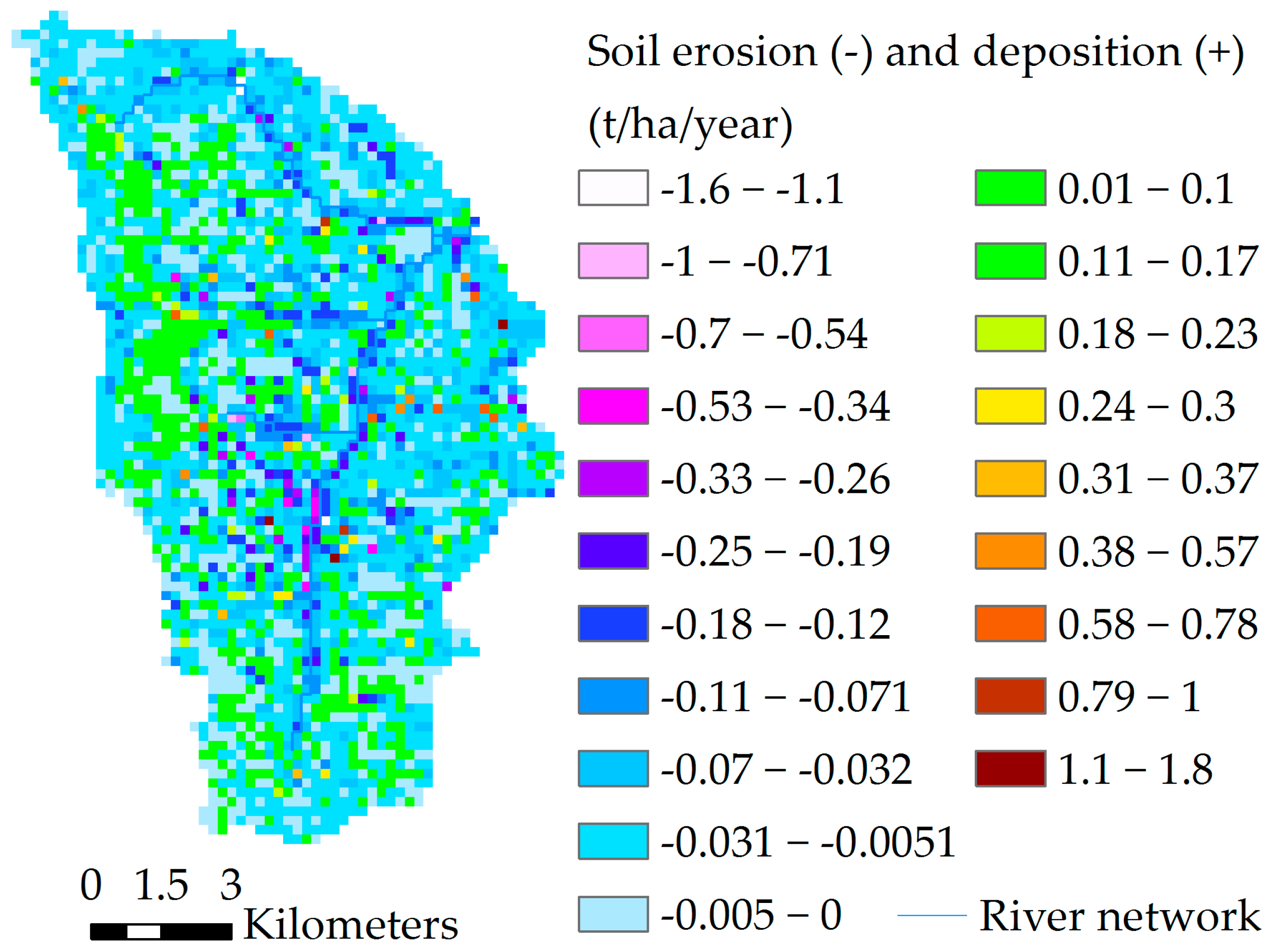
Catchment Distributed Erosion

Figure 6 shows the spatial pattern of soil erosion and deposition on hillslopes as simulated by the best SHETRAN simulation for the calibration period. Erosion ranges from 1.6 to almost 0 t/ha/year and deposition from 0 to 1.8 t/ha/year. Regarding erosion 55% of the grid cells are within the range of −0.03 to <0 t/ha/year. However, given the spatial heterogeneity of the controlling factors that are considered (slope, land use, soil properties, hydrological conditions) and the complex model approach it is difficult to clearly identify erosion hot spots and to explicitly attribute these hot spots to a single factor or reason. One example in this context is the hilly area in the western part of the catchment: We assumed the highest erosion rates would be found here due to the steep slopes and the partly practiced agriculture but simulated erosion is not especially high compared with other parts of the catchment. The small erosion rates are attributed to the low simulated surface runoff due to a small drainage area of these cells. Hence, rain drop detachment may be high but surface runoff is insufficient to transport the available sediment. High erosion rates simulated close to the river channel are a result of higher surface runoff simulated in cells close to the valley bottoms as a result of larger drainage areas and overbank flow. Field observations confirm overbank flow during large events but the areas are rather characterized by deposition of fine material and not necessarily by erosion as simulated. To get a more realistic representation of the vegetation close to the rivers (gallery forests), a fifth land use type with the same properties as savannah vegetation was introduced around the river links. Though this led to lower erosion rates, it negatively affected the performance of the simulated hydrograph and was therefore discarded.

4. Conclusions

This study applied the hydrological soil erosion model SHETRAN in a tropical West African catchment and investigated measurement and parameter uncertainty. From the investigations we can draw the following conclusions:

(1)

The performed uncertainty analyses of observed discharge reveals large uncertainty bands especially during peak flows (max. uncertainty from 17.3 (−34.1% of measured value) to 40.3 m³/s (+53.1% of measured value)) which was attributed on the one hand to the power law chosen for the rating curves and on the other hand to the sample properties. As a result of the intrinsic measurement errors and the error propagation the combined uncertainty of SSL is quite large (max. uncertainty from 2.8 to 8 kg/s).

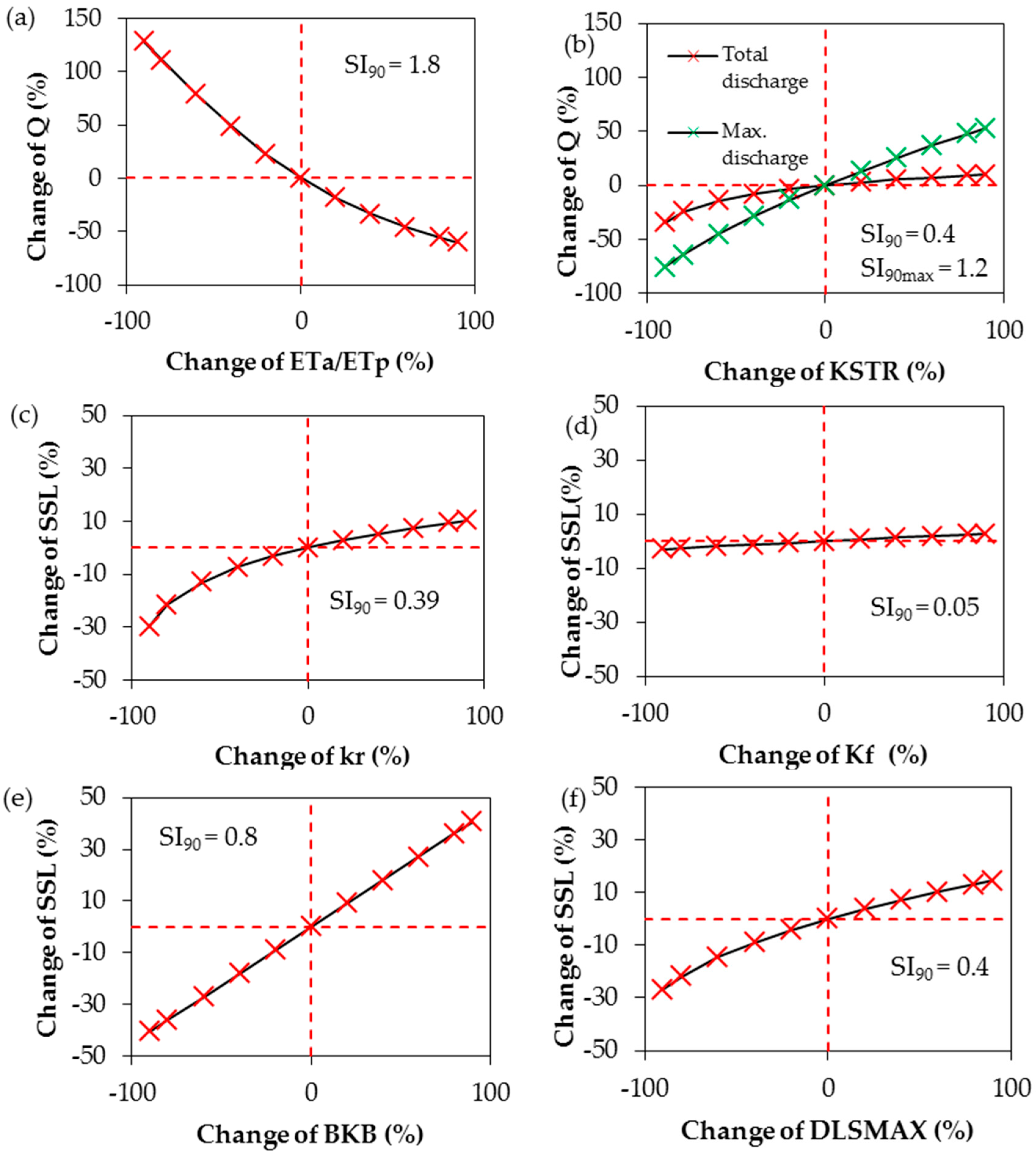
(2)

Two hydrological parameters were tested regarding the sensitivity of the model response. Whereas the ratio ETa/ETp affects total catchment runoff, the roughness coefficient KSTR has greater effect on the maximum runoff. Among the four tested erosion related model parameters the river bank erodibility coefficient BKR had the largest impact on the model response. Parameter ranges of the overland flow erodibility coefficient k_f and DLSMAX were quite low which was explained by the higher soil erodibility of the soils found in the study area.

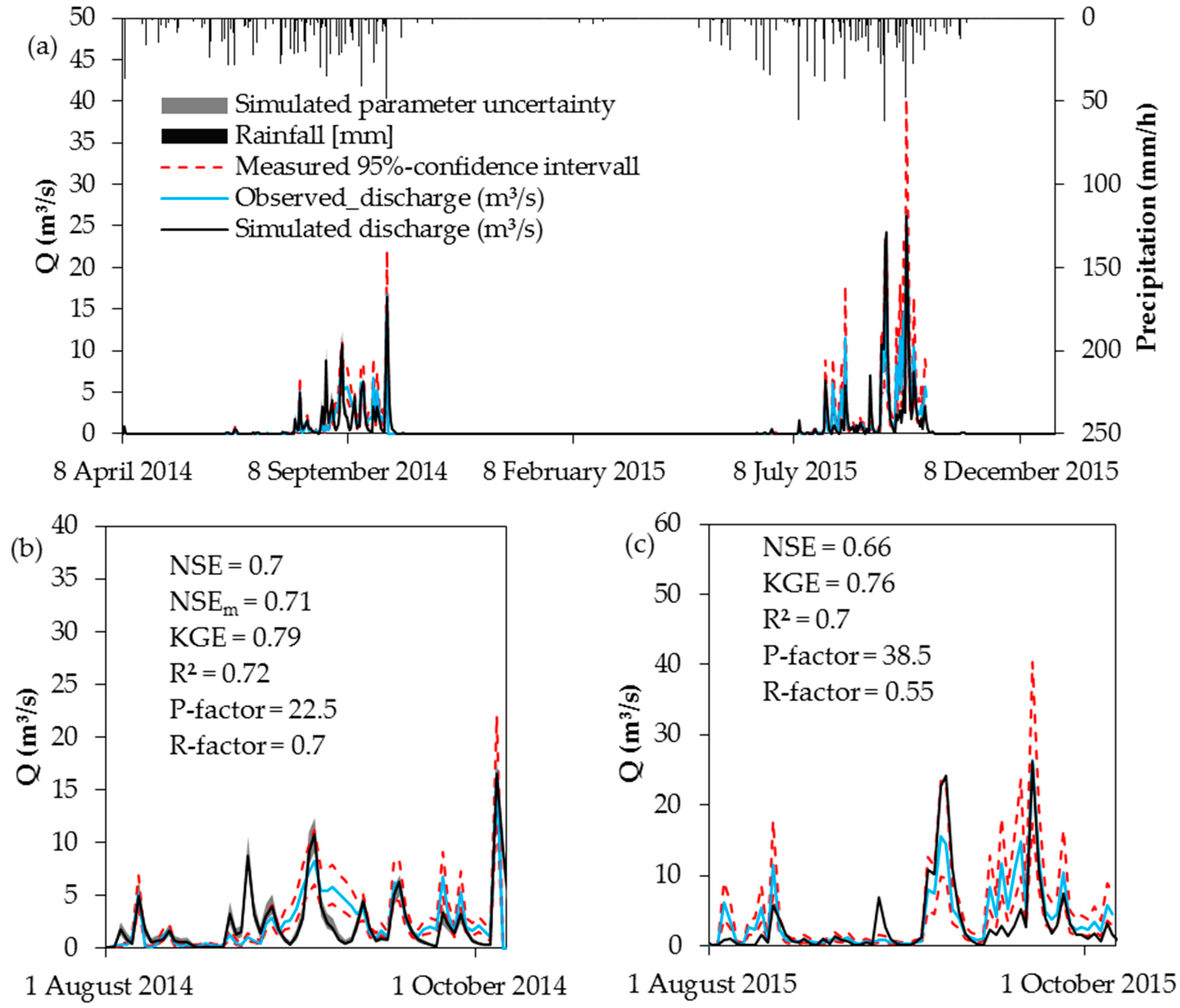
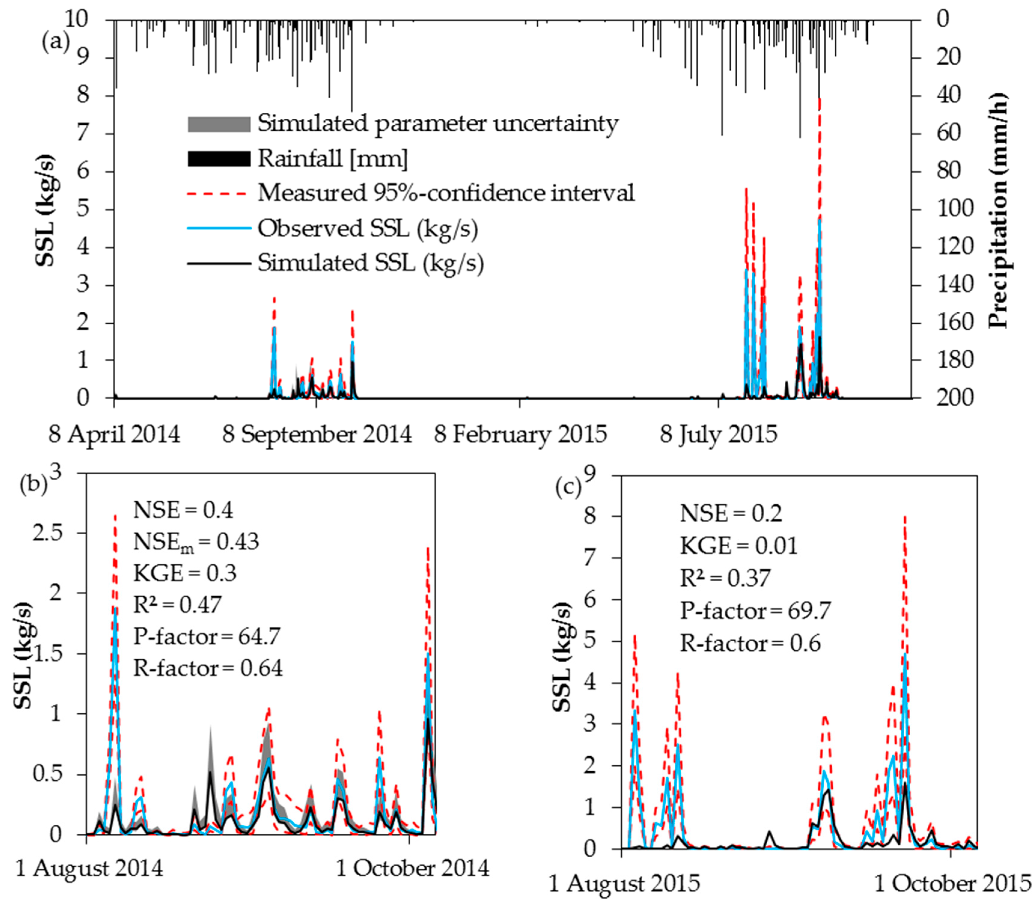
(3)

The performance indices of simulated discharge are good (≥0.66) and comparable with other studies that used SHETRAN. Among these studies R² and NSE values above 0.5 are frequently reported. However, SHETRAN often underestimates base flow which could be explained by the missing calibration of hydrological subsurface parameters. Some peaks were not well represented due to the differences between real and model spatial representation of rainfall. The performance indices of the simulated SSL are comparable with the few studies that used SHETRAN to simulate soil erosion and that indicated model performance. As the calculation of SSC is based on the relation between turbidity and sediment concentration, input of organic material into the river following the burning of crop residues and grassland may lead to high turbidity readings although the measured weight is low [91,92]. Thus, the mismatch between observed and simulated SSL at the start of the rainy season may also be explained by the method used to obtain the sedigraph.

(4)

The combined uncertainty assessment of measured and simulated discharge showed that SHETRAN frequently underestimates base flow despite large measured uncertainty bounds. The modified NSE_m used to include both uncertainties in the quality assessment showed that the overlapping areas of distributions are rarely observed and small. As a result of the large uncertainty of observed SSL the model uncertainty is almost always within the range of measured uncertainty bounds. This is also reflected by a slightly higher NSE_m in comparison with the traditional NSE. The erosion sources simulated by SHETRAN do not correspond with the sources reported in the literature. The contribution of river bank and bed erosion may be too high and the erosion on hillslopes too low. However, knowledge on this point is limited. Results from fingerprint analyses may help to validate the simulated output.

We showed that the physically based spatially distributed erosion model SHETRAN offers chances and challenges. SHETRAN provides a better representation of erosion processes, especially in environments that are characterized by low frequency and high magnitude erosion events, than low-complexity models that focus on mean annual erosion rates (such as the USLE). So far, the application to larger river catchments is limited due to the incomplete knowledge on the model parameters and the limited availability of model input data at a large scale and with appropriate resolution. Yet, the modeling results obtained here help to improve the parameterization of large-scale, low-complexity erosion models and to improve the representation of the strong temporal variability of erosion rates in the Sudano savanna zone of Africa. Consequently, modeling erosion on a small scale is needed to optimize parameter estimation and process understanding which in turn helps to improve large scale modeling [93]. Erosion modeling with SHETRAN should therefore focus on better and broader knowledge on the erosion parameters, including the definition of parameter ranges for different environmental conditions. The application of SHETRAN to erosion plots may be an opportunity to better assess these parameter values.

References

1. Bationo, A.; Kihara, J.; Vanlauwe, B.; Waswa, B.; Kimetu, J. Soil organic carbon dynamics, functions and management in West African agro-ecosystems. Agric. Syst. 2007, 94, 13–25. [Google Scholar] [CrossRef]
2. Lal, R. Soil degradation by erosion. Land Degrad. Dev. 2001, 12, 519–539. [Google Scholar] [CrossRef]
3. Toy, T.J.; Foster, G.R.; Renard, K.G. Soil Erosion: Processes, Prediction, Measurement, and Control; John Wiley & Sons: Hoboken, NJ, USA, 2002. [Google Scholar]
4. United Nations Environmental Programme. Global Environment Outlook 4; UNEP: Valletta, Malta, 2012; p. 551. [Google Scholar]
5. Morgan, R.P.C. Soil Erosion and Conservation; Blackwell Publishing: Oxford, UK, 2005. [Google Scholar]
6. Okou, F.A.Y.; Tente, B.; Bachmann, Y.; Sinsin, B. Regional erosion risk mapping for decision support: A case study from West Africa. Land Use Policy 2016, 56, 27–37. [Google Scholar] [CrossRef]
7. Smith, P.; House, J.I.; Bustamante, M.; Sobocká, J.; Harper, R.; Pan, G.; West, P.C.; Clark, J.M.; Adhya, T.; Rumpel, C.; et al. Global change pressures on soils from land use and management. Glob. Chang. Biol. 2016, 22, 1008–1028. [Google Scholar] [CrossRef] [PubMed] [Green Version]
8. De Vente, J.; Poesen, J.; Verstraeten, G.; Govers, G.; Vanmaercke, M.; Van Rompaey, A.; Arabkhedri, M.; Boix-Fayos, C. Predicting soil erosion and sediment yield at regional scales: Where do we stand? Earth Sci. Rev. 2013, 127, 16–29. [Google Scholar] [CrossRef]
9. Pandey, A.; Himanshu, S.K.; Mishra, S.K.; Singh, V.P. Physically based soil erosion and sediment yield models revisited. Catena 2016, 147, 595–620. [Google Scholar] [CrossRef]
10. Lal, R. Soil Erosion Research Methods; CRC Press: Boca Raton, FL, USA, 1994. [Google Scholar]
11. Ewen, J.; Parkin, G.; O’Connell, P.E. SHETRAN: Distributed river basin flow and transport modeling system. J. Hydrol. Eng. 2000, 5, 250–258. [Google Scholar] [CrossRef]
12. Wicks, J.M.; Bathurst, J.C. SHESED: A physically based, distributed erosion and sediment yield component for the SHE hydrological modelling system. J. Hydrol. 1996, 175, 213–238. [Google Scholar] [CrossRef]
13. Birkinshaw, S.J.; Bathurst, J.C. Model study of the relationship between sediment yield and river basin area. Earth Surf. Process. Landf. 2006, 31, 750–761. [Google Scholar] [CrossRef]
14. Đukić, V.; Radić, Z. Sensitivity Analysis of a Physically Based Distributed Model. Water Resour. Manag. 2016, 30, 1669–1684. [Google Scholar] [CrossRef]
15. Ewen, J.; O’Donnell, G.; Burton, A.; O’Connell, E. Errors and uncertainty in physically-based rainfall-runoff modelling of catchment change effects. J. Hydrol. 2006, 330, 641–650. [Google Scholar] [CrossRef]
16. Beven, K.; Freer, J. Equifinality, data assimilation, and uncertainty estimation in mechanistic modelling of complex environmental systems using the GLUE methodology. J. Hydrol. 2001, 249, 11–29. [Google Scholar] [CrossRef]
17. Rompaey, A.J.; Govers, G. Data quality and model complexity for regional scale soil erosion prediction. Int. J. Geogr. Inf. Sci. 2002, 16, 663–680. [Google Scholar] [CrossRef]
18. Harmel, R.D.; Smith, P.K. Consideration of measurement uncertainty in the evaluation of goodness-of-fit in hydrologic and water quality modeling. J. Hydrol. 2007, 337, 326–336. [Google Scholar] [CrossRef]
19. Navratil, O.; Esteves, M.; Legout, C.; Gratiot, N.; Nemery, J.; Willmore, S.; Grangeon, T. Global uncertainty analysis of suspended sediment monitoring using turbidimeter in a small mountainous river catchment. J. Hydrol. 2011, 398, 246–259. [Google Scholar] [CrossRef]
20. Rasmussen, P.P.; Gray, J.R.; Glysson, G.D.; Ziegler, A.C. Guidelines and Procedures for Computing Time-Series Suspended-Sediment Concentrations and Loads from In-Stream Turbidity-Sensor and Streamflow Data; U.S. Geological Survey: Reston, VA, USA, 2009.
21. Rode, M.; Suhr, U. Uncertainties in selected river water quality data. Hydrol. Earth Syst. Sci. 2007, 11, 863–874. [Google Scholar] [CrossRef]
22. Kusimi, J.M.; Yiran, G.A.; Attua, E.M. Soil Erosion and Sediment Yield Modelling in the Pra River Basin of Ghana using the Revised Universal Soil Loss Equation (RUSLE). Ghana J. Geogr. 2016, 7, 38–57. [Google Scholar]
23. Bossa, A.; Diekkrüger, B.; Agbossou, E. Scenario-Based Impacts of Land Use and Climate Change on Land and Water Degradation from the Meso to Regional Scale. Water 2014, 6, 3152–3181. [Google Scholar] [CrossRef]
24. Obeta, I.N.; Adewumi, J.K. Soil Loss in Samaru Zaria Nigeria: A comparison of WEPP and EUROSEM Models. Niger. J. Technol. 2013, 32, 197–202. [Google Scholar]
25. Schmengler, A.C. Modeling Soil Erosion and Reservoir Sedimentation at Hillslope and Catchment Scale in Semi-Arid Burkina Faso. Ph.D. Thesis, Rheinische Friedrich-Wilhelms-Universität, Bonn, Germany, 2010. [Google Scholar]
26. Hiepe, C. Soil Degradation by Water Erosion in a Sub-Humid West-African Catchment—A Modelling Approach Considering Land Use and Climate Change in Benin. Ph.D. Thesis, Rheinische Friedrich-Wilhelms-Universität, Bonn, Germany, 2008. [Google Scholar]
27. Visser, S.M.; Sterk, G.; Karssenberg, D. Modelling water erosion in the Sahel: Application of a physically based soil erosion model in a gentle sloping environment. Earth Surf. Process. Landf. 2005, 30, 1547–1566. [Google Scholar] [CrossRef]
28. Karambiri, H.; Ribolzi, O. Identification of sediment sources in a small grazed Sahelian catchment, Burkina Faso. In Sediment Budgets 1; Walling, D.E., Horowitz, A., Eds.; IAHS Press: Wallingford, UK, 2005; p. 291. [Google Scholar]
29. Mati, B.M.; Veihe, A. Application of the USLE in a Savannah Environment: Comparative Experiences from East and West Africa. Singap. J. Trop. Geogr. 2001, 22, 138–155. [Google Scholar] [CrossRef]
30. Igwe, C.A.; Mbagwu, J.S.C. Application of SLEMSA and USLE models for potential erosion hazard mapping in South-Eastern Nigeria. Int. Agrophys. 1999, 13, 41–48. [Google Scholar]
31. Roose, E.J. Use of the Universal Soil Loss Equation to Predict Erosion in West Africa; Soil Conservation Society of America: Ankeny, IA, USA, 1977; pp. 60–74. [Google Scholar]
32. Đukić, V.; Radić, Z. GIS Based Estimation of Sediment Discharge and Areas of Soil Erosion and Deposition for the Torrential Lukovska River Catchment in Serbia. Water Resour. Manag. 2014, 28, 4567–4581. [Google Scholar] [CrossRef]
33. Zhang, R. Integrated Modelling for Evaluation of Climate Change Impacts on Agricultural Dominated Basin. Ph.D. Thesis, University Evora, Evora, Portugal, 2015. [Google Scholar]
34. Mourato, S.; Moreira, M.; Corte-Real, J. Water Resources Impact Assessment under Climate Change Scenarios in Mediterranean Watersheds. Water Resour. Manag. 2015, 29, 2377–2391. [Google Scholar] [CrossRef]
35. Naseela, E.K.; Dodamani, B.M.; Chandran, C. Estimation of Runoff Using NRCS-CN Method and SHETRAN Model. Int. Adv. Res. J. Sci. Eng. Technol. 2015, 2, 23–28. [Google Scholar]
36. Birkinshaw, S.J.; Bathurst, J.C.; Robinson, M. 45 years of non-stationary hydrology over a forest plantation growth cycle, Coalburn catchment, Northern England. J. Hydrol. 2014, 519, 559–573. [Google Scholar] [CrossRef]
37. Tripkovic, V. Quantifying and Upscaling Surface and Subsurface Runoff and Nutrient Flows under Climate Variability. Ph.D. Thesis, Newcastle University, Newcastle upon Tyne, UK, 2014. [Google Scholar]
38. Elliott, A.H.; Oehler, F.; Schmidt, J.; Ekanayake, J.C. Sediment modelling with fine temporal and spatial resolution for a hilly catchment. Hydrol. Process. 2011, 26, 3645–3660. [Google Scholar] [CrossRef]
39. Bathurst, J.C.; Birkinshaw, S.J.; Cisneros, F.; Fallas, J.; Iroumé, A.; Iturraspe, R.; Novillo, M.G.; Urciuolo, A.; Alvarado, A.; Coello, C.; et al. Forest impact on floods due to extreme rainfall and snowmelt in four Latin American environments 2: Model analysis. J. Hydrol. 2011, 400, 292–304. [Google Scholar] [CrossRef]
40. Birkinshaw, S.J.; Bathurst, J.C.; Iroumé, A.; Palacios, H. The effect of forest cover on peak flow and sediment discharge—An integrated field and modelling study in central-southern Chile. Hydrol. Process. 2010, 25, 1284–1297. [Google Scholar] [CrossRef]
41. De Figueiredo, E.E.; Bathurst, J.C. Runoff and sediment yield predictions in a semiarid region of Brazil using SHETRAN. In Proceedings of the PUB Kick-Off Meeting, Brasilia, Brazil, 20–22 November 2002; International Association of Hydrological Sciences (IAHS) Publications: Wallingford, UK, 2007; Volume 309. [Google Scholar]
42. Adams, R.; Parkin, G.; Elliott, S.; Rutherford, K. Modelling of hillslope erosion from New Zealand pasture using a rainfall simulator. In Proceedings of the British Hydrological Society International Conference, London, UK, 2004; pp. 415–420.
43. Norouzi Banis, Y.; Bathurst, J.C.; Walling, D.E. Use of caesium-137 data to evaluate SHETRAN simulated long-term erosion patterns in arable lands. Hydrol. Process. 2004, 18, 1795–1809. [Google Scholar] [CrossRef]
44. Anderton, S.P.; Latron, J.; White, S.M.; Llorens, P.; Gallart, F.; Salvany, C.; O’Connell, P.E. Internal evaluation of a physically-based distributed model using data from a Mediterranean mountain catchment. Hydrol. Earth Syst. Sci. Discuss. 2002, 6, 67–84. [Google Scholar] [CrossRef] [Green Version]
45. Lukey, B.; Sheffield, J.; Bathurst, J.; Hiley, R.; Mathys, N. Test of the SHETRAN technology for modelling the impact of reforestation on badlands runoff and sediment yield at Draix, France. J. Hydrol. 2000, 235, 44–62. [Google Scholar] [CrossRef]
46. Callo-Concha, D.; Gaiser, T.; Ewert, F. Farming and Cropping Systems in the West African Sudanian Savanna. WASCAL Research Area: Northern Ghana, Southwest Burkina Faso and Northern Benin; ZEF Working Paper Series; Center for Development Research: Bonn, Germany, 2012. [Google Scholar]
47. Comité Inter-États de Lutte Contre la Sécheresse Dans le Sahel. Landscapes of West Africa—A Window on a Changing World; U.S. Geological Survey EROS: Garretson, SD, USA, 2016.
48. Gleisberg-Gerber, K. Livelihoods and Land Management in the Ioba Province in South-Western Burkina Faso; ZEF Working Paper Series; Center for Development Research: Bonn, Germany, 2012. [Google Scholar]
49. Yira, Y.; Diekkrüger, B.; Steup, G.; Bossa, A.Y. Modeling land use change impacts on water resources in a tropical West African catchment (Dano, Burkina Faso). J. Hydrol. 2016, 537, 187–199. [Google Scholar] [CrossRef]
50. Schmengler, A.C.; Vlek, P.L. Assessment of accumulation rates in small reservoirs by core analysis, 137Cs measurements and bathymetric mapping in Burkina Faso. Earth Surf. Process. Landf. 2015, 40, 1951–1963. [Google Scholar] [CrossRef]
51. International Union of Soil Sciences (IUSS) Working Group. World Reference Base for Soil Resources 2006, 2nd ed.; World Soil Resources Reports; Food and Agriculture Organization: Rome, Italy, 2006; Volume 103. [Google Scholar]
52. Jarvis, A.; Reuter, H.I.; Nelson, A.; Guevara, E. Hole-Filled SRTM for the Globe Version. 2008. Available online: http://srtm.csi.cgiar.org (accessed on 1 August 2014).
53. Forkuor, G. Agricultural Land Use Mapping in West Africa Using Multi-Sensor Satellite Imagery. Ph.D. Thesis, Julius-Maximilians-Universität, Würzburg, Germany, 2014. [Google Scholar]
54. Abbott, M.B.; Bathurst, J.C.; Cunge, J.A.; O’Connell, P.E.; Rasmussen, J. An introduction to the European Hydrological System—Systeme Hydrologique Europeen, “SHE”, 1: History and philosophy of a physically-based, distributed modelling system. J. Hydrol. 1986, 87, 45–59. [Google Scholar] [CrossRef]
55. Wicks, J.M. Physically-Based Mathematical Modelling of Catchment Sediment Yield. Ph.D. Thesis, Newcastle University, Newcastle upon Tyne, UK, 1988. [Google Scholar]
56. Parkin, G. A three-Dimensional Variably-Saturated Subsurface Modelling System for River Basins. Ph.D. Thesis, Newcastle University, Newcastle upon Tyne, UK, 1996. [Google Scholar]
57. Bathurst, J.C. Predicting Impacts of Land Use and Climate Change on Erosion and Sediment Yield in River Basins Using SHETRAN. In Handbook of Erosion Modelling; John Wiley & Sons, Ltd.: Hoboken, NJ, USA, 2010; pp. 263–288. [Google Scholar]
58. Monteith, J.L. Vegetation and the Atmosphere, Vol. 1: Principles, Vol. 2: Case Studies; Academic Press: New York, NY, USA, 1975. [Google Scholar]
59. Feddes, R.A.; Kowalik, P.; Neuman, S.P.; Bresler, E. Finite Difference and Finite Element Simulation of Field Water Uptake by Plants. Hydrol. Sci. J. 1976, 21, 81–98. [Google Scholar]
60. Rutter, A.J.; Morton, A.J.; Robins, P.C. A Predictive Model of Rainfall Interception in Forests. II. Generalization of the Model and Comparison with Observations in Some Coniferous and Hardwood Stands. J. Appl. Ecol. 1975, 12, 367–380. [Google Scholar] [CrossRef]
61. Rutter, A.J.; Kershaw, K.A.; Robins, P.C.; Morton, A.J. A predictive model of rainfall interception in forests, 1. Derivation of the model from observations in a plantation of Corsican pine. Agric. Meteorol. 1972, 9, 367–384. [Google Scholar] [CrossRef]
62. Van Genuchten, M.T. A closed-form equation for predicting the hydraulic conductivity of unsaturated soils. Soil Sci. Soc. Am. J. 1980, 44, 892–898. [Google Scholar] [CrossRef]
63. Rawls, W.J.; Brakensiek, D.L. Prediction of soil water properties for hydrologic modeling. In Watershed Management in the Eighties; Amer Society of Civil Engineers (ASCE): Reston, VA, USA, 1985; pp. 293–299. [Google Scholar]
64. Brakensiek, D.L.; Rawls, W.J. Soil containing rock fragments: Effects on infiltration. Catena 1994, 23, 99–110. [Google Scholar] [CrossRef]
65. Birkinshaw, S.J. Technical Note: Automatic river network generation for a physically-based river catchment model. Hydrol. Earth Syst. Sci. 2010, 14, 1767–1771. [Google Scholar] [CrossRef]
66. Wicks, J.M.; Bathurst, J.C.; Johnson, C.W.; Ward, T.J. Application of two physically-based sediment yield models at plot and field scales. In Sediment Budgets (Proceedings of the Porto-Alegre Symposium); IASH Press: Wallingford, UK, 1988; pp. 583–591. [Google Scholar]
67. Ariathurai, R.; Arulanandan, K. Erosion rates of cohesive soils. J. Hydraul. Div. 1978, 104, 279–283. [Google Scholar]
68. Osman, A.M.; Thorne, C.R. Riverbank stability analysis. I: Theory. J. Hydraul. Eng. 1988, 114, 134–150. [Google Scholar] [CrossRef]
69. Engelund, F.; Hansen, E. A Monograph on Sediment Transport in Alluvial Streams; Polyteknisk Forlag: Copenhagen, Denmark, 1967. [Google Scholar]
70. Ackers, P.; White, W.R. Sediment transport: New approach and analysis. J. Hydraul. Div. 1973, 99, 2041–2060. [Google Scholar]
71. Morgan, R.P.C.; Nearing, M.A. Handbook of Erosion Modelling; Wiley Online Library: Oxford, UK, 2011. [Google Scholar]
72. De Roo, A.P.J. Modelling Surface Runoff and Soil Erosion in Catchments Using Geographical Information Systems: Validity and Applicability of the “answers” Model in Two Catchments in the Loess Area of South Limburg (The Netherlands) and one in Devon (UK). Ph.D. Thesis, Rijksuniversiteit Utrecht, The Netherlands, 1993. [Google Scholar]
73. McKay, M.D.; Beckman, R.J.; Conover, W.J. A Comparison of Three Methods for Selecting Values of Input Variables in the Analysis of Output from a Computer Code. Technometrics 1979, 21, 239–245. [Google Scholar] [CrossRef]
74. Nash, J.E.; Sutcliffe, J.V. River flow forecasting through conceptual models part I—A discussion of principles. J. Hydrol. 1970, 10, 282–290. [Google Scholar] [CrossRef]
75. Gupta, H.V.; Kling, H.; Yilmaz, K.K.; Martinez, G.F. Decomposition of the mean squared error and NSE performance criteria: Implications for improving hydrological modelling. J. Hydrol. 2009, 377, 80–91. [Google Scholar] [CrossRef]
76. Kling, H.; Fuchs, M.; Paulin, M. Runoff conditions in the upper Danube basin under an ensemble of climate change scenarios. J. Hydrol. 2012, 424, 264–277. [Google Scholar] [CrossRef]
77. Shuttleworth, W.J. Evaporation. In Handbook of Hydrology; Maidment, D.R., Ed.; McGraw-Hill: New York, NY, USA, 1993. [Google Scholar]
78. Mohamoud, Y.M. Evaluating Manning’s roughness coefficients for tilled soils. J. Hydrol. 1992, 135, 143–156. [Google Scholar] [CrossRef]
79. Shen, H.W.; Julien, P.Y. Erosion and sediment transport. In Handbook of Hydrology; Maidment, D.R., Ed.; McGraw-Hill: New York, NY, USA, 1993. [Google Scholar]
80. Adams, R.; Elliott, S. Physically based modelling of sediment generation and transport under a large rainfall simulator. Hydro. Process. 2006, 20, 2253–2270. [Google Scholar] [CrossRef]
81. Lukey, B.T.; Sheffield, J.; Bathurst, J.C.; Lavabre, J.; Mathys, N.; Martin, C. Simulating the effect of vegetation cover on the sediment yield of mediterranean catchments using SHETRAN. Phys. Chem. Earth 1995, 20, 427–432. [Google Scholar] [CrossRef]
82. Helsel, D.R.; Hirsch, R.M. Statistical methods in water resources. In Hydrologic Analysis and Interpretation; U.S. Geological Survey: Reston, VA, USA, 2002. [Google Scholar]
83. Abbaspour, K.C.; Faramarzi, M.; Ghasemi, S.S.; Yang, H. Assessing the impact of climate change on water resources in Iran. Water Resour. Res. 2009, 45. [Google Scholar] [CrossRef]
84. Harmel, R.D.; Smith, P.K.; Migliaccio, K.W. Modifying goodness-of-fit indicators to incorporate both measurement and model uncertainty in model calibration and validation. Trans. ASABE 2010, 53, 55–63. [Google Scholar] [CrossRef]
85. Bathurst, J.C.; Ewen, J.; Parkin, G.; O’Connell, P.E.; Cooper, J.D. Validation of catchment models for predicting land-use and climate change impacts. 3. Blind validation for internal and outlet responses. J. Hydrol. 2004, 287, 74–94. [Google Scholar] [CrossRef]
86. Parkin, G.; O’donnell, G.; Ewen, J.; Bathurst, J.C.; O’Connell, P.E.; Lavabre, J. Validation of catchment models for predicting land-use and climate change impacts. 2. Case study for a Mediterranean catchment. J. Hydrol. 1996, 175, 595–613. [Google Scholar] [CrossRef]
87. Minella, J.P.G.; Merten, G.H.; Reichert, J.M.; Clarke, R.T. Estimating suspended sediment concentrations from turbidity measurements and the calibration problem. Hydrol. Process. 2008, 22, 1819–1830. [Google Scholar] [CrossRef]
88. Nearing, M.A. Why soil erosion models over-predict small soil losses and under-predict large soil losses. Catena 1998, 32, 15–22. [Google Scholar] [CrossRef]
89. Walling, D.E.; Collins, A.L.; Sichingabula, H.M.; Leeks, G.J.L. Integrated assessment of catchment suspended sediment budgets: A Zambian example. Land Degrad. Dev. 2001, 12, 387–415. [Google Scholar] [CrossRef]
90. Hoffmann, T. Sediment residence time and connectivity in non-equilibrium and transient geomorphic systems. Earth Sci. Rev. 2015, 150, 609–627. [Google Scholar] [CrossRef]
91. Gippel, C. The use of turbidimeters in suspended sediment research. Hydrobiologia 1989, 176, 465–480. [Google Scholar] [CrossRef]
92. Gippel, C.J. Potential of turbidity monitoring for measuring the transport of suspended solids in streams. Hydrol. Process. 1995, 9, 83–97. [Google Scholar] [CrossRef]
93. Panagos, P.; Borrelli, P.; Poesen, J.; Meusburger, K.; Ballabio, C.; Lugato, E.; Montanarella, L.; Alewell, C. Reply to the comment on “The new assessment of soil loss by water erosion in Europe” by Fiener & Auerswald. Environ. Sci. Policy 2016, 57, 143–150. [Google Scholar]
Figure 1. Location map of the Dano catchment: (a) location of the catchment and Burkina Faso in West Africa; (b) slope of the catchment; (c) model catchment; (d) land use map [53]; (e) soil map (data base: soil survey done by Ozias Hounkpatin, University of Bonn, Institute of Crop Science and Resource Conservation, Soil Science and Soil Ecology).
Water 09 00101 g001
Figure 2. Scatter plots of recorded water level and measured water discharge for (a) 2014 (n = 6); and (b) 2015 (n = 10) and of (c) the recorded turbidity and measured suspended sediment concentration (SSC) (n = 57).
Water 09 00101 g002
Figure 3. Scatter plots showing the sensitivity of water discharge Q to the ratio of actual to potential evapotranspiration (ETa/ETp) (a); and surface roughness (KSTR) (b); and the sensitivity of the catchment suspended sediment load (SSL) to the raindrop erodibility coefficient (kr) (c); the overland flow erodibility (kf) (d); the bank erodibility (BKB) (e); and the depth of loose sediment (DLSMAX) (f). Red dashed lines indicate the base run used for comparison. SI90max indicates the SI90 for the maximum discharge.
Water 09 00101 g003
Figure 4. Observed and simulated daily discharge (Q) over the calibration and validation period (a); and over a selected period for the calibration (b); and validation (c) period. The measured 95%-confidence interval is given for both periods, simulated parameter uncertainty only for the calibration year.
Water 09 00101 g004
Figure 5. Observed and simulated daily suspended sediment load (SSL) over the calibration and validation period (a); and a selected period for the calibration (b); and validation (c) period. Measurement uncertainty is given for both periods, parameter uncertainty only for the calibration.
Water 09 00101 g005
Figure 6. Annual soil erosion (-) and deposition rate (+) on hillslopes as simulated for the calibration period.
Water 09 00101 g006